The quantum Kibble-Zurek mechanism: the role of boundary conditions, endpoints and kink types

Jose Soto Garcia^1$\star$ and Natalia Chepiga^1$\dagger$

Abstract

Quantum phase transitions are characterised by the universal scaling laws in the critical region surrounding the transitions. This universality is also manifested in the critical real-time dynamics through the quantum Kibble-Zurek mechanism. In recent experiments on a Rydberg atom quantum simulator, the Kibble-Zurek mechanism has been used to probe the nature of quantum phase transitions. In this paper we analyze the caveats associated with this method and develop strategies to improve its accuracy. Focusing on two minimal models—transverse-field Ising and three-state Potts—we study the effect of boundary conditions, the location of the endpoints and some subtleties in the definition of the kink operators. In particular, we show that the critical scaling of the most intuitive types of kinks is extremely sensitive to the correct choice of endpoint, while more advanced types of kinks exhibit remarkably robust universal scaling. Furthermore, we show that when kinks are tracked over the entire chain, fixed boundary conditions improve the accuracy of the scaling. Surprisingly, the Kibble-Zurek critical scaling appears to be equally accurate whether the fixed boundary conditions are chosen to be symmetric or anti-symmetric. Finally, we show that the density of kinks extracted in the central part of long chains obeys the predicted universal scaling for all types of boundary conditions.

Copyright attribution to authors.
This work is a submission to SciPost Physics.
License information to appear upon publication.
Publication information to appear upon publication. Received Date
Accepted Date
Published Date

 

Contents

1. 1 Introduction
2. 2 The Models
   1. 2.1 Transverse Field Ising Model
   2. 2.2 3-state Potts Model
   3. 2.3 Three-State Potts Model
3. 3 Methods
   1. 3.1 Ground State Calculations
   2. 3.2 Simulation of dynamics
4. 4 System Size
5. 5 Types of kinks and the endpoint
6. 6 Boundary Conditions
7. 7 Conclusion and Discussion

 

1 Introduction

Understanding the nature of quantum phase transitions is a central challenge in condensed matter physics. Unlike classical transitions, which are driven by thermal fluctuations, quantum phase transitions (QPTs) appear due to quantum fluctuations, offering a unique perspective on the fundamental mechanisms of critical phenomena [1].

Traditionally, the critical exponents characterizing QPTs have been investigated in equilibrium [2]. However, the discovery of the Kibble-Zurek (KZ) mechanism [3, 4, 5, 6] has opened new pathways to explore the interplay between non-equilibrium dynamics and critical phenomena. Near the critical point of a continuous phase transition, the correlation length $\xi$ and healing time $\tau$ diverge with the distance to the transition $g_{c}$ following a power law scaling[5]:

$$\xi \sim\absolutevalue{g-g_{c}}^{-\nu},$$ (1)

$$\tau \sim\absolutevalue{g-g_{c}}^{-\nu\tau}.$$ (2)

When a system is driven with a constant sweep rate $s$ from a disordered phase to an ordered one crossing a continuous phase transition, its dynamics become non-adiabatic when the temporal distance to the critical point matches the system’s healing time. This results in the emergence of quasiparticle excitations—kinks $n_{k}$. In one dimension, kinks correspond to domain walls between ordered regions, and their average spacing is directly related to the correlation length of the system. Theory predicts that sufficiently far from the transition, the density of kinks scales as a power law with the sweep rate [5]:

$$n_{k}\sim s^{-d\mu},$$ (3)

with $d$ is the dimensionality of the system and $\mu$ is Kibble-Zurek critical exponent that can be expressed as a function of the critical exponent $\nu$ and the dynamical critical exponent $z$:

$$\mu=\frac{\nu}{1+\nu z}.$$ (4)

Initially proposed by Kibble to explain structure formation in the early universe [7, 8], the symmetry-breaking framework was later extended by Zurek to classical [9] and quantum phase transitions [3, 4, 10] in condensed matter systems. While the original hypothesis stated that the system freezes at the onset of the non-adiabatic regime [3], subsequent research has shown that this is not totally correct. Instead, the system continues evolving, with correlations spreading across the system through the dispersion of the quasiparticle excitations [11, 12, 13, 14].

Experimental progress in platforms of Rydberg atoms [15] have brought renewed attention to the experimental study of quantum many-body systems, and in particular, to non-equilibrium critical phenomena[6], spurring extensive numerical [16, 17, 18, 19, 20, 21] and experimental [22, 23, 24, 25, 26, 27, 28, 29, 30] studies of the quantum KZ mechanism. However, despite the power law scaling of the KZ mechanism being observed, the obtained critical exponents tend to differ from the theoretical predictions. Competing effects during the KZ protocol are believed to interfere with the results, pushing them away from the theoretical expectations[31, 32].

The remainder of this article is organized as follows. In Section 2, we introduce the two models studied in this work: the transverse field Ising model and the 3-state Potts model. Section 3 provides a concise review of the Tensor Network algorithms used in our simulations, along with relevant technical details. In Section 4, we investigate the influence of system size on the Kibble–Zurek mechanism. Section 5 presents an alternative approach to counting kinks by focusing exclusively on isolated kinks, and we show that this method is more robust to changes in the final point of the sweep through the transition. In Section 6, we compare various boundary conditions, demonstrating that fixing the boundaries—either on the same or in different directions—yields more accurate results than leaving them free. Finally, Section 7 summarizes our findings and offers concluding remarks.

2 The Models

We explore the role of boundary conditions and the effectiveness of various definitions of kinks in two well established microscopic quantum models: The antiferromagnetic transverse field Ising model (TFIM) and the 3-state Potts model in 1D.

2.1 Transverse Field Ising Model

The quantum TFIM is defined by the following microscopic Hamiltonian:

$$H=J\sum_{i=1}^{L-1}\sigma^{z}_{i}\sigma^{z}_{i+1}-h\sum_{i=1}^{L}\sigma^{x}_{i},$$ (5)

where $\sigma^{z,x}$ represents the Pauli matrices, $J$ is the nearest-neighbor Ising coupling, and $h$ is an external magnetic field in the transverse direction. The model is ferromagnetic when $J<0$ and antiferromagnetic when $J>0$. In this paper we focus on the latter case. The location of the critical point $h/J=1$ is known exactly along with all relevant critical exponents: $z=1$, $\nu=1$, $\mu=1/2$[33]. To control the boundary conditions we also included a magnetic field in the first and last lattice sites along the $z-$direction.

$$H=H_{0}-(h_{z1}\sigma^{z}_{1}+h_{zL}\sigma^{z}_{L}).$$ (6)

For the antiferromagnetic TFIM ($J>0$), the standard number of kinks operator is defined as:

$$n_{k}=\frac{1}{2}\sum_{i=1}^{L-1}\left(1+\sigma^{z}_{i}\sigma^{z}_{i+1}\right),$$ (7)

which assigns 1 for each pair of aligned neighboring spins (i.e., a ‘kink’ in the otherwise alternating antiferromagnetic configuration).

2.2 3-state Potts Model

The ferromagnetic 3-states Potts model is a generalization of the ferromagnetic TFIM for the local Hilbert space of dimension three. The microscopic Hamiltonian is given by:

$$H=-J\sum_{i=1}^{L-1}\sum_{a=1}^{3}P_{i}^{a}P_{i+1}^{a}-h\sum_{i=1}^{L}P_{i},$$ (8)

where $P_{i}^{a}=\ket{a}\bra{a}_{i}-1/3$ is the projector of the spin at site $i$ along the direction $a$, and $P_{i}=\ket{\lambda_{0}}\bra{\lambda_{0}}-1/3$ the projector of the spin along the direction $\ket{\lambda_{0}}=1/\sqrt{3}\sum_{a}\ket{a}$. The first term represents a ferromagnetic interaction, and the second term represents a generalized transverse field. The critical point is located at $h/J=1$ and has critical exponents $\nu=5/6$ and $z=1$, and thus $\mu\approx 0.454$[33]. Similarly to TFIM, boundaries can be controlled by adding an external longitudinal field:

$$H=H_{0}-\sum_{a=1}^{3}\left(h_{a1}P^{a}_{1}+h_{aL}P^{a}_{L}\right).$$ (9)

The kink operator has the form:

$$n_{k}=\sum_{i=1}^{L-1}\left(1-\sum_{a}(\ket{a}\bra{a})_{i}\cdot(\ket{a}\bra{a})_{i+1}\right),$$ (10)

where $(\ket{a}\bra{a})_{i}$ is the projector onto state $\ket{a}$ at site i. Thus $n_{k}$ counts a kink whenever two neighboring sites differ. For simplicity, we will refer to three possible directions as $A$, $B$ and $C$.

2.3 Three-State Potts Model

The ferromagnetic three-state Potts model generalizes the ferromagnetic TFIM to a local Hilbert space of dimension three. Its microscopic Hamiltonian is given by:

$$H=-J\sum_{i=1}^{L-1}\sum_{a=1}^{3}P_{i}^{a}P_{i+1}^{a}\;-\;h\sum_{i=1}^{L}P_{i},$$ (11)

where

$$P_{i}^{a}=\ket{a}\bra{a}_{i}-\tfrac{1}{3}$$

is the projector onto state $\ket{a}$ (with $a\in\{1,2,3\}$) at site $i$, and

$$P_{i}=\ket{\lambda_{0}}\bra{\lambda_{0}}_{i}-\tfrac{1}{3},\quad\text{where }\ket{\lambda_{0}}=\frac{1}{\sqrt{3}}\sum_{a=1}^{3}\ket{a},$$

is the projector onto the equally weighted superposition $\ket{\lambda_{0}}$. The first sum (involving $J$) encodes the ferromagnetic interaction, while the second (involving $h$) acts as a generalized transverse field. At the critical point $h/J=1$, the model has critical exponents $\nu=5/6$ and $z=1$, yielding $\mu\approx 0.454$ [33].

Similarly to the TFIM, boundary conditions can be adjusted by adding an external longitudinal field:

$$H=H_{0}-\sum_{a=1}^{3}\bigl{(}h_{a1}\,P^{a}_{1}\;+\;h_{aL}\,P^{a}_{L}\bigr{)}.$$ (12)

We define the standard kink operator as

$$n_{k}=\sum_{i=1}^{L-1}\biggl{(}1\;-\;\sum_{a=1}^{3}(\ket{a}\bra{a})_{i}\,(\ket{a}\bra{a})_{i+1}\biggr{)},$$ (13)

where $(\ket{a}\bra{a})_{i}$ is the projector onto state $\ket{a}$ at site $i$. Thus $n_{k}$ counts a kink whenever two neighboring sites differ. For simplicity, we refer to the three possible states as $A$, $B$, and $C$.

3 Methods

3.1 Ground State Calculations

The initial state defined at time $t=0$ is a ground state at a given starting point in the disordered phase sufficiently far from the transition. The ground state was determined using the density matrix renormalization group (DMRG) algorithm[34, 35]. Singular values were kept above $10^{-6}$, and maximal bond dimension was restricted to $D=300$. Convergence of the ground state was assumed when the relative energy difference between two successive sweeps, including an increase in the bond dimension, was not exceeding $10^{-9}$.

3.2 Simulation of dynamics

Simulations of the time evolution for the TFIM with open boundary conditions and 3-state Potts model were conducted using a second-order time-evolving block decimation (TEBD) algorithm [36, 37, 38]. The time step was fixed at $\delta=0.1$, with the maximum dimension set to $D=300$ and the singular value cutoff maintained at $\chi>10^{-6}$. In Figure 1 we compare various values of $D$ for the TFIM (Figure 1(a)) and the 3-state Potts Model (Figure 1(b)). In both cases, the Kibble-Zurek exponent $\mu$ remains robust for moderately small bond dimensions, showing visible deviations only for very small $D$.

For simulations employing periodic boundary conditions, the time-dependent variational principle (TDVP) [39, 40, 38] was used instead, while retaining the same values of $D$ and $\chi$ as in TEBD.

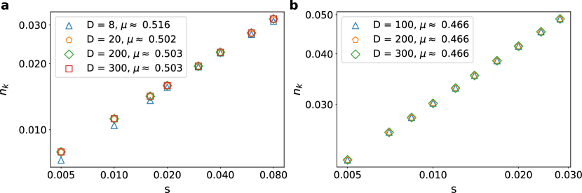
Figure 1: Kibble-Zurek scaling of the density of kinks $n_{k}$ as a function of the sweep rate for various bond dimensions $D$ in (a) the transverse-field Ising model (TFIM) and (b) the 3-state Potts model. Simulation of Kibble-Zurek dynamics requires relatively small bond dimension ($D\lesssim 100$). For the rest of the simulations $D=300$ was used for both Ising and 3-state Potts models.

4 System Size

First, we studied the role of finite-size effects in the Kibble-Zurek (KZ) mechanism in both models. Figure 2(a) summarizes our results for the Ising model, for which we examined a broad spectrum of sweep rates $s$ to capture the full range of dynamical behaviors. Three distinct regimes are clearly visible: For slow sweep rates, the correlation length becomes comparable to the system size, and the system evolves adiabatically during the whole process. Here, the density of kinks remains nearly zero and does not depend on the sweep rate [10, 5]. For very rapid sweeps, the evolution is entirely non-adiabatic. In this case, the density of kinks saturates to a maximum value determined by the final point of the quench [41, 42]. Between the adiabatic and fast quench limit there is an interval of the KZ scaling regime, characterized by a power-law dependence of the density of kinks as a function of the sweep rate.

For the TFIM, increasing the system size does not notably affect the exponent $\mu$ associated with the KZ scaling—nearly all system sizes, except $L=30$, yield the same $\mu$. However, the threshold sweep rate at which the slope is linear decreases as the system size grows, extending the interval over which the KZ mechanism can be observed.

For the 3-state Potts model (Figure 2(b)), we focus directly on the Kibble-Zurek region. By contrast to the Ising model, here the slope of the critical scaling shows finite-size effect and slowly approaches from above the theoretical value $\mu=5/11$ in the thermodynamic limit. For $L=401$ sites numerically extracted value of the critical exponent $\mu\approx 0.463$ agrees within 2$\%$ with the theory predictions.

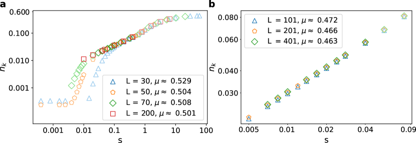
Figure 2: Kibble-Zurek scaling of the kink density $n_{k}$ as a function of the sweep rate $s$ for different system sizes in (a) the Ising and (b) the 3-state Potts models. (a) Three distinct regimes are visible in the data. At slow sweep rates, the system remains adiabatic, and the kink density stays around zero. As the sweep rate increases, an intermediate region emerges where $n_{k}$ follows a universal power-law scaling with $s$. At even faster sweep rates, the system evolves in the non-adiabatic regime, causing the kink density to saturate at a constant value. Results for system sizes with 50 sites demonstrate excellent agreement with theory predictions $\mu=0.5$. (b) Kibble-Zurek scaling for the the 3-state Potts model. We observe a small finite-size effect resulting in the overestimated value of the critical exponent $\mu$. For $L=401$ sites our numerical result agree with the theory prediction $\mu=5/11$ within $2\%$. Data points not included in the KZ fit are shown in pale.

5 Types of kinks and the endpoint

The standard protocol for extracting the KZ exponent $\mu$ consists of driving the system from the disordered phase into the ordered phase and counting the number of kinks after the transition for various sweep rates. In a first approximation, the system freezes upon entering the non-adiabatic regime, and the correlation length (that in 1D is directly related to the density of kinks) remains fixed thereafter. However, it has been shown that this approximation is oversimplified: the system continues to evolve and correlations continue to spread even as it crosses the critical point [11, 12, 13, 14]. In the transverse-field Ising model (TFIM), a more refined picture involves the creation of entangled kinks pairs with opposite momenta that spread correlations along the system.

Moreover, during the dynamics, quantum coarsening competes with the KZ mechanism, further increasing the correlation length [32]. As a result, the correlation length continues to increase even after the system has returned to the adiabatic regime. Finally, if the transverse field is not completely suppressed, there is a certain probability of a local spin flip. Thus not all the detected kinks arise from the KZ mechanism itself.

In this section, we analyze two factors that affect the calculation of the KZ critical exponent $\mu$: the endpoint where the dynamics terminate and the choice of a kink operator. All results presented in this section were obtained with fixed boundary conditions, while the effect of various boundary conditions on the apparent KZ critical exponent will be discussed in detail in the next section. We consider two types of kink definitions as sketched in Figure 3, for the TFIM with antiferromagnetic (Figure 3(a)-(c)) and ferromagnetic (Figure 3(d)-(f)) interactions. In the standard definition, a kink is counted whenever the expected order is violated. For instance, in the ferromagnetic case, a kink is counted if any pair of neighboring spins are anti-aligned, while in the antiferromagnetic case, it is counted if they are aligned (see Figure 3(d) and (a) correspondingly).

Alternatively, one can count only isolated kinks, thus excluding configurations in which more than two consecutive spins deviate from the expected order. In the antiferromagnetic case, this means disregarding regions where three or more neighboring spins are aligned instead of alternating, as shown in 3(b). In the ferromagnetic case, it entails excluding regions where three or more spins are anti-align, as depicted in 3(e). Such scenarios are typical for a single-spin flip, as shown Figure 3(c) and (f). Under the conventional definition [5], such a single flip would count as two kinks. However, since a local flip is not a true domain wall but rather an impurity within a single domain, it should be excluded from the final count.

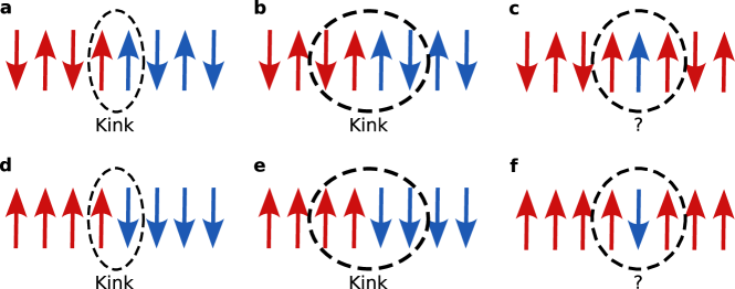
Figure 3: Kinks and domain walls in the Ising model with (a)-(c) antiferromagnetic and (d)-(e) ferromagnetic interactions. Red and blue colors are assigned to each of the two ground-states. (a),(d) In the standard definition [5], kinks are counted every time the expected order is violated. (b),(e) Kinks computed over four consecutive spins ensures that the domains on each site of the kink has at least length two. (c),(f) Spin-flip is counted as a double-kink in the standard definition. In this work we propose to exclude a single-spin flip contribution from kinks as it does not change the nature of the domain.

Figure 4(a) shows the critical scaling of the density of standard kinks with a sweep rate for three different endpoints: $h_{e}=0$ and $h_{e}=\pm 0.2$. While the KZ exponent extracted for the trajectory terminating at $h_{e}=0$ is in excellent agreement with the theory prediction for Ising criticality $\mu=0.5$, critical exponents extracted for other endpoints deviate significantly. If instead we use an advanced definition of kinks where a single-spin flip is explicitly excluded from the kink counting, extremely accurate values of KZ exponents have been extracted from time-evolution to all three endpoints, as demonstrated in Figure 4(b). This means that local impurities, which are not real domain walls, do not play a role in the Kibble-Zurek dynamics and must generally be filtered out by a proper definition of the kink operators. Alternatively, one can terminate the dynamical evolution at the point where the quantum term responsible for the local spin flip is absent, and such impurities do not appear.

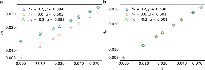
Figure 4: Scaling of the density of kinks $n_{k}$ with the sweep rate $s$ for the Ising model for various final values of the transverse field $h_{e}$ using (a) the standard kinks operator, (b) a kink operator that only counts isolated domain walls (i.e. excludes local spin flips). The Kibble-Zurek exponent $\mu$ is extracted from the slope of the power law scaling. (a) Numerically extracted $\mu$ using the standard kink operator agrees with the theory prediction $\mu=0.5$ only for $h_{e}=0$, while the value of $\mu$ extracted with other endpoints is significantly underestimated. (b) The scaling of isolated kinks provides accurate numerical estimates of the Kibble-Zurek critical exponent $\mu$ for a wide range of final endpoints. In both cases, the system size is $L=201$.

This logic of robust kinks can be extended beyond the trivial Ising model, as shown in Figure 5. However, for the 3-state Potts model, the definition of a robust kink is more subtle, since the spin flip might or might not lead to a switch of domain walls, as shown in Figure 5(c)-(d). In this case, the advanced definition of kink discards spin flips inside a domain (Figure 5(c)), but treats a spin flip that bridges two different domains as a single kink (Figure 5(d)).

Figure 5: Domain wall characterization on the 3-state Potts model. (a) Simple kinks are counted when two consequtive sites are in two different local states. (b) Domain walls are only counted when two spins pointing to different directions are aligned with their nearest neighbours. (c) A spin-flip is counted as a double-kink in the standard definition, but it is excluded in the new definition since it does not change the nature of the domain. (d) A spin-flip between different domains is again counted as a double kink in the standard definition. However, in the new definition it is only counted as one kink, since there are only two real domains.

This way of counting kinks in the 3-state Potts model yields results comparable to those of the the TFIM, as shown in Figure 6. Using the standard kink definition the Kibble-Zurek exponent $\mu$ is closes to its theoretical value when the sweep ends at zero transverse field $h_{e}=0$, where no dynamical term is present. If the sweep terminates before or after this sweet spot, $\mu$ is noticeably underestimated, as illustrated in Figure 6(a). In contrast, the advanced kink definition (Figure 6(b)) is more robust to the ending point, causing the three curves to overlap and yielding a more accurate $\mu$. In all cases, the density of kinks scales as a power law dependence on the sweep rate.

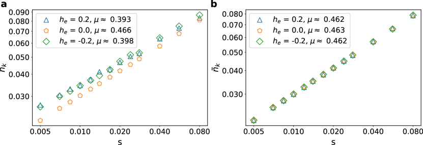
Figure 6: Scaling of the density of kinks $n_{k}$ with the sweep rate $s$ for the 3-state Potts model for various final values of the transverse field using (a) the standard kinks operator, (b) a kink operator that only counts isolated domain walls. The Kibble-Zurek exponent $\mu$ is extracted from the slope of the power law scaling. With the simple kink operator, only $\mu$ extracted for the trajectory that ends at $h_{e}=0$ is reasonably close (within 3$\%$) to the theoretical value $\mu=0.454$ for 3-state Potts, while other endpoints significantly reduce the the slope. When using the isolated kink operator, numerically extracted value agree within $2\%$ with the theory prediction for a wide range of endpoints. In both presented cases the system size is $L=201$.

In Figure 7 we present the profiles of the local density of kinks for the Ising and 3-state Potts models for various endpoints for a single sweep rate. Direct comparison between the standard and isolated kinks allows one to reveal that all profiles obtained for the same sweep rate and system size but ending at various points are very similar up to a constant shift caused apparently by single-flip excitations as the shift is completely gone for the isolated kinks where all curves appear on top of each other.

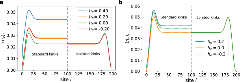
Figure 7: Local density of kinks $n_{k}$ along the chain for (a) the Ising and (b) the 3-state Potts models for various values of the final transverse field $h_{e}$. Each plot is split in two: in the left side, the kink operator is the standard domain wall operator, while in the right side only isolated kinks are measured. For both, Ising and Potts models, when $h_{e}=0$ the profiles of standard and isolated kinks coincide. However, for different end points the profile of standard kinks is shifted, while the profile for isolated kinks remains robust.

In the 3-state Potts model, we can also compare the local density of spin flips inside or between domains for $h_{e}=0$ and $h_{e}\neq 0$. Figure 8 illustrates these scenarios: panel (a) shows the local density profiles for both types of spin flips when $h_{e}=0$, and panel (b) shows them when $h_{e}=0.2$. As expected from Figure 7, spin flips occur more frequently under nonzero $h_{e}$. Moreover, even though flipping a spin inside a domain costs twice as much energy as flipping one at a domain boundary, such “in-domain” flips are still more common. The apparent contradiction is resolved by noting that domain walls are relatively rare, making it statistically more likely for a random spin to be inside a domain rather than at its boundary.

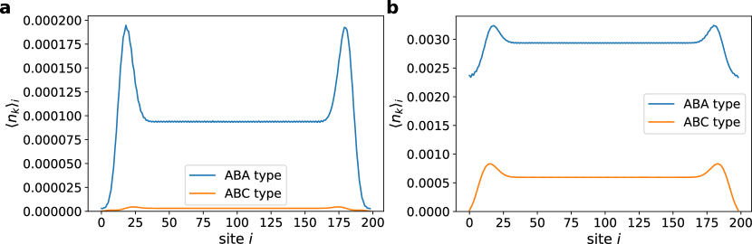
Figure 8: Local density of two types of local kinks $n_{k}$ in the 3-state Potts model, shown along the chain for (a) $h_{e}=0$ and (b) $h_{e}=0.2$. The blue curve corresponds to spin flips inside a domain, and the orange curve to spin flips at a domain boundary. In both cases spin flips inside a domain are more abundant than at a domain boundary.

Finally, let us compare the evolution of the overall density of standard and isolated kinks in the whole quench protocol. The results for the Ising model are presented in Figure 9. Let us carefully explain this figure. When $h\rightarrow\infty$, the ground state is $\ket{...+++++...}$. The density of kinks in this maximally disordered state is $n_{k}=0.5$ while isolated kinks is $n_{k}=0.125$. This number can be easily obtained by counting the number of domain walls or isolated domain walls respectively in the perfectly disordered state (i.e. number of aligned pairs of spins or isolated aligned pairs of spins in the antiferromagnetic TFIM). As we approach the phase transition at $h=1$, but still far from the non-adiabatic regime, the average number of kinks decreases, while the density of isolated ones remains constant. Around the phase transition there is a rapid decrease on the density of kinks, as ordered domains separated by few domain walls arise. The density of standard kinks gets a minima at $h=0$, where quantum fluctuations are only due to the KZ mechanism, and increases thereafter. The density of isolated kinks, however, reaches their minimum value before $h=0$ and remain constant for a long range of values of $h$ before and after $h=0$. The isolated kink operator is therefore resilient against random quantum fluctuations and only measures domain walls due to the KZ mechanism.

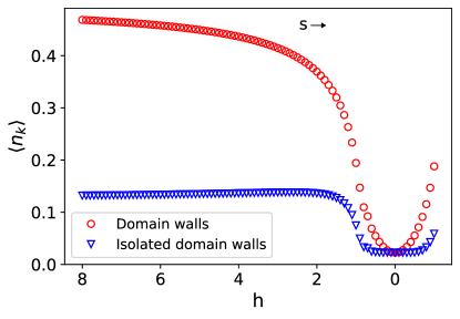
Figure 9: Evolution of the kink density $n_{k}$ during a constant-rate quench in the TFIM, comparing the standard kink-counting method (red circles) to counting only isolated kinks (blue triangles), where isolated means that single spin flips are not counted. Deep in the disordered phase ($h\gg 1$), the density of kinks reaches its maximum ($n_{k}=0.5$ for the standard definition and $n_{k}=0.125$ for isolated kinks). As the system crosses the phase transition at $h=1$, the emergence of large ordered regions leads to a sudden drop in the kink density. At $h=0$, both counting methods yield the same minimal density, since any remaining kinks are solely due to domain wall creation as described by the KZ mechanism. Notably, while isolated kinks maintain their minimal density over a wide range of $h$, the standard kink definition only attains this minimal value at $h=0$.

6 Boundary Conditions

The critical properties of a quantum system depend not only on the bulk Hamiltonian but also on its boundary conditions, and the same holds true for its dynamical behavior. To investigate whether boundary conditions influence the apparent Kibble–Zurek exponent, we examined the scaling of kink densities for both the TFIM and the 3-state Potts model under various boundary conditions. Our results for the two models are summarized in Figure 10 and Figure 11 correspondingly. For this, we evaluate the density of kinks in two different ways: over the entire chain including the edges, and over a small interval in the middle of the chain. In this section we present results obtained with $L=201$ and we use the standard definition of kinks (see previous section for details). We polarized boundary conditions by applying an external longitudinal magnetic field.

For the Ising model, we examine five different boundary conditions: boundary conditions fixed at both edges of the chain in a symmetric $h_{z1}=h_{zL}=10$ or antisymmetric $h_{z1}=-h_{zL}=10$ way; weakly polarized boundary conditions with $h_{z1}=h_{zL}=0.1$; free boundary conditions ($h_{z1}=h_{zL}=0$); and the boundary condition fixed at one edge and free at another one $h_{z1}=0$ and $h_{zL}=10$. Our results are summarized in Figure 10. When kinks are counted in the small central interval ($\approx 10\%$ of the total length) of a long chain, the density of kinks evaluated for all five boundary conditions scales with a KZ critical exponent that agrees within $2\%$ with the theory expectation $\mu=0.5$. If instead, the density of kinks was evaluated over the entire chain (as it is often the case in experiments where available system sizes are limited) the critical exponent evaluated with the fixed boundary conditions turns out to be significantly more accurate. As a big surprise, we observe no difference in KZ dynamics with fixed symmetric and fixed antisymmetric boundary conditions for which equilibrium properties are drastically different.

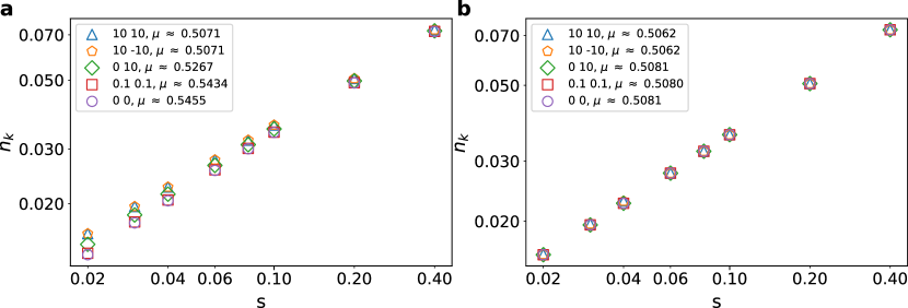
Figure 10: Scaling of the density of kinks $n_{k}$ with the sweep rate $s$ for the Ising model for various boundary conditions when measuring the density of kinks (a) over the entire chain (b) over the central $10\%$ of the chain. The boundary conditions were fixed with external longitudinal field applied at first and last site of the chain and indicated in the legends. The results evaluated in the central part of the chain always agree within 2$\%$ with the theory prediction $\mu=1/2$, while the results evaluated over the entire chain provide more accurate estimate of the KZ exponent when the boundary conditions are fixed.

For the ferromagnetic 3-state Potts model, we also examine five different boundary conditions: fixed boundary conditions favoring the same (A A) or different (A B) ferromagnetic state at each edge; free (0 0) and fixed-free (A 0) boundary conditions. These four boundary conditions are direct generalization of the boundary conditions considered for the Ising model. In addition, we also consider mixed boundary conditions (AB AB) obtained by applying positive longitudinal field in the C direction at each edge. The results obtained with these boundary conditions are summarized in Figure 11. Similar to the Ising, case we see that when the KZ exponent is extracted from the total density of kinks, the results obtained with fixed boundary conditions are significantly more accurate than those obtained with other types of boundaries (see Figure 11(a)). If, however, the density of kinks is evaluated only in the central interval of a long enough chain, the boundary conditions do not matter, just like we have observed for the Ising model in Figure 10(b).

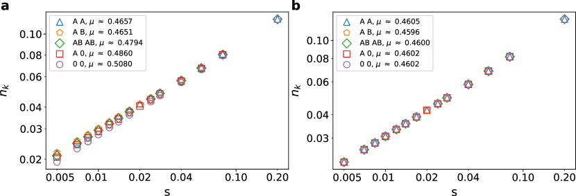
Figure 11: Scaling of the density of kinks $n_{k}$ with the sweep rate $s$, in the 3-sate Potts model for various boundary conditions when the density of kinks is measured (a) over the whole chain, and (b) over the central $10\%$ interval of the chain. Fixed boundary conditions are labeled with A or B, mixed with AB (not-C), free boundary is marked with 0. The results evaluated in the central part of the chain always agree within 2$\%$ with the theory prediction $\mu=5/11$, while the results evaluated over the entire chain provide more accurate estimate of the KZ exponent when the boundary conditions are fixed.

We also examine the scenario of periodic boundary conditions (PBC). In Figure 12, we compare the scaling of the kink density for the antiferromagnetic TFIM under PBC for two system sizes, $L=200$ (the system size compatible with the periodicity of the ground state) and $L=201$ (the system size non-compatible with the ground-state periodicity, often called anti-periodic boundary conditions in the field-theory context). We see that $\mu$ is independent of this choice.

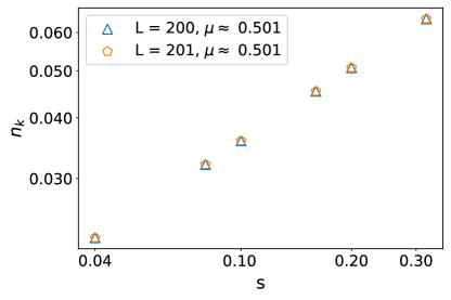
Figure 12: Comparison of the kink density scaling for the transverse-field Ising model under periodic boundary conditions (PBC) when the system size is compatible (blue markers) and when it is incompatible (orange markers) with the periodicity of the ground state. Two data sets demonstrate a remarkable overlap.

In Figure 13 we demonstrate the distribution of local density of kinks along the chain under various boundary conditions for the TFIM (Figure 13(a)) and the 3-state Potts model (Figure 13(b)). Both models exhibit remarkably similar kink distributions when subjected to the same boundary conditions. For the periodic boundaries, the kink distribution, as expected, is uniform across the chain. For open and fixed boundaries—whether fixed in the same or opposite directions—kinks tend to accumulate near, but not directly adjacent to, the boundaries, reaching zero at the edges. Remarkably, the total number of kinks is the same for fixed and periodic boundary conditions, with only the distribution being affected.

When boundaries are open but free, the peak in the kink distribution observed for fixed boundaries disappears, although the kinks density still decreases toward the boundaries. Under these conditions, the total number of kinks is reduced compared to the fixed boundary conditions.

Finally, for the mixed boundaries in the Potts model—where the degree of freedom is partially constrained at the edges, such that local state C is disfavored, while A and B can appear with equal probability—the peak in the kink distribution is smaller than in the fixed case. Here, the total number of kinks falls between those for free and fixed boundary conditions. And, as we have seen in Figure 11 the accuracy of the KZ exponent also lies in between the fixed and free cases.

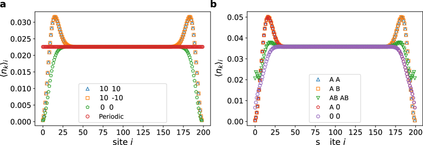
Figure 13: Distribution of kinks along the chain for (a) the TFIM and (b) the 3-state Potts model for various boundary conditions listed in the legend.

The last question that we are going to explore is the optimal length of the central interval of the chain to evaluate the KZ exponent. Figure 14 provides the value of the KZ exponent $\mu$ as a function of the relative discarded interval at each edge of the chain with $L=201$ sites while computing the density of kinks for various boundary conditions.

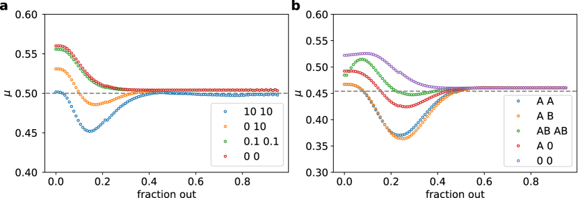
Figure 14: Kibble-Zurek exponent as a function of the fraction of the edge discarded for density calculations for various boundary conditions for (a) The TFIM and (b) the 3-state Pots model. Dashed lines indicate theory predictions $\mu=0.5$ for TFIM and $\mu=5/11$ for 3-state Potts model.

Ising and 3-state Potts models show a similar behaviour. In both cases the $\mu$ matches the theoretical value for the whole chain when boundaries are fixed. For all boundary conditions the edge effects seem to vanish after half of the considered chains (in other words, about 100 sites) are discarded. This interval is expected to be model dependent, but already this simple examples of the two minimal models provides us with a good indication that one has to discard many dozes of sites posting quite a significant lower bound on the total length of the chain.

7 Conclusion and Discussion

In this paper we have studied the effect of boundary conditions in space and time and the role they play in quantum Kibble-Zurek mechanism as a tool to probe quantum phase transitions.

Our main finding is that the accuracy of the Kibble-Zurek mechanism in the naive implementation is extremely sensitive to the location of the final point—the point where the time evolution terminates and the measurements are performed. Our data show that, for the two minimal models considered here, the best choice of the final point would be the point where the transverse field responsible for quantum fluctuations vanishes. If the final measurement point deviates from this classical limit, whether it lies before or after the zero-transverse-field point, the observed critical exponent $\mu$ deviates markedly from the theoretically predicted universal value

Interestingly enough, exactly the same type of fine-tuning to the classical end point has been realized in Rydberg simulators. In the experiment, after quenching through a quantum phase transition, the Rabi frequency $\Omega$ responsible for quantum fluctuations of atoms between the ground-state and excited Rydberg state has to be turned off to perform the read-outs. The only difference between the two protocols is a path to reach this specific end point. In the minimal models considered above, we quenched the transverse field itself to the point when it vanishes. In experiments, one quenches either the laser detuning (this would corresponds to an additional longitudinal field in the minimal models) or the combination of the detuning and Rabi frequency to an arbitrary point inside the ordered phase and then turns off the lasers responsible for the resonance. Importantly, in both protocols, the transition is crossed with a linear ramp. Numerical simulations that closely reproduce the experimental protocol demonstrate excellent agreement with the expected universal scaling at the Ising and Potts points[21].

Such fine-tuning of the final point is natural for experiments on Rydberg atoms, but may not be generic in other contexts. In this paper, we present an alternative approach based on a more careful definition of the kink operator, which demonstrates a remarkable robustness to the location of the final endpoint. In this approach, the kink represents a domain wall between two extended domains, excluding, in particular, localized excitations within the domain of the same ground-state, like a single-spin flip. This definition requires some level of book-keeping but admits a conceptually straightforward generalization to other more complex models.

In addition, we investigated how different boundary conditions affect the accuracy of the critical scaling. For both minimal models considered, we find that the accuracy of the Kibble-Zurek critical exponent is systematically improved for fixed boundary conditions with respect to the free ones. Surprisingly, we observe no difference in critical dynamics performed with symmetric and anti-symmetric (in the conformal field theory sense) fixed boundary conditions, despite their drastic differences in equilibrium scenarios. In effective models of Rydberg atoms, the presence of a longitudinal field (arising from laser detuning) partially fixes the boundary conditions by favoring the excitation of edge atoms into Rydberg states. Increasing the laser detuning at the edges can further reinforce these effective fixed boundary conditions. The lack of any difference between symmetric and anti-symmetric boundary conditions relaxes experimental constraints. Typically, arrays with a total size $N=kp+1$ with $k\in\mathbb{Z}$ have been used to probe the transition into the period-$p$ phase. Our results suggest that the scaling should be universal for any values of $N$ (of course, $N$ has to be big enough to host the Kibble-Zurek regime).

We also report that, for sufficiently long chains, the universal Kibble-Zurek scaling can be accurately extracted by calculating the density of kinks in the central part of the chain, thus ignoring the effect of the boundaries. The size of the chain in this case must be substantially larger than the resulting correlation length after a quench, which naturally increases with decreasing sweep rate. For the minimal models and sweep rates considered here, the edge effects are significant over the first 30-40 sites, imposing a lower bound on the total chain length of at least $N\gtrsim 100$ sites. These lengths are feasible but challenging in modern Rydberg experiments, so fixing the boundary conditions seems to be the best strategy for now.

References

- [1] S. Sachdev, Quantum phase transitions, Physics world 12(4), 33 (1999).
- [2] J. Cardy, Scaling and renormalization in statistical physics, vol. 5, Cambridge university press (1996).
- [3] W. H. Zurek, U. Dorner and P. Zoller, Dynamics of a quantum phase transition, Physical review letters 95(10), 105701 (2005).
- [4] A. Polkovnikov, Universal adiabatic dynamics in the vicinity of a quantum critical point, Phys. Rev. B 72, 161201 (2005), 10.1103/PhysRevB.72.161201.
- [5] J. Dziarmaga, Dynamics of a quantum phase transition and relaxation to a steady state, Advances in Physics 59(6), 1063 (2010).
- [6] A. Keesling, A. Omran, H. Levine, H. Bernien, H. Pichler, S. Choi, R. Samajdar, S. Schwartz, P. Silvi, S. Sachdev et al., Quantum kibble–zurek mechanism and critical dynamics on a programmable rydberg simulator, Nature 568(7751), 207 (2019).
- [7] T. W. Kibble, Topology of cosmic domains and strings, Journal of Physics A: Mathematical and General 9(8), 1387 (1976).
- [8] T. W. Kibble, Some implications of a cosmological phase transition, Physics Reports 67(1), 183 (1980).
- [9] W. H. Zurek, Cosmological experiments in superfluid helium?, Nature 317(6037), 505 (1985).
- [10] J. Dziarmaga, Dynamics of a quantum phase transition: Exact solution of the quantum ising model, Physical review letters 95(24), 245701 (2005).
- [11] M. Kolodrubetz, B. K. Clark and D. A. Huse, Nonequilibrium dynamic critical scaling of the quantum ising chain, Physical review letters 109(1), 015701 (2012).
- [12] A. Chandran, A. Erez, S. S. Gubser and S. L. Sondhi, Kibble-zurek problem: Universality and the scaling limit, Physical Review B—Condensed Matter and Materials Physics 86(6), 064304 (2012).
- [13] A. Francuz, J. Dziarmaga, B. Gardas and W. H. Zurek, Space and time renormalization in phase transition dynamics, Physical Review B 93(7), 075134 (2016).
- [14] D. Sadhukhan, A. Sinha, A. Francuz, J. Stefaniak, M. M. Rams, J. Dziarmaga and W. H. Zurek, Sonic horizons and causality in phase transition dynamics, Physical Review B 101(14), 144429 (2020).
- [15] H. Bernien, S. Schwartz, A. Keesling, H. Levine, A. Omran, H. Pichler, S. Choi, A. S. Zibrov, M. Endres, M. Greiner et al., Probing many-body dynamics on a 51-atom quantum simulator, Nature 551(7682), 579 (2017).
- [16] P. Laguna and W. H. Zurek, Density of kinks after a quench: When symmetry breaks, how big are the pieces?, Physical Review Letters 78(13), 2519 (1997).
- [17] H. Saito, Y. Kawaguchi and M. Ueda, Kibble-zurek mechanism in a quenched ferromagnetic bose-einstein condensate, Physical Review A—Atomic, Molecular, and Optical Physics 76(4), 043613 (2007).
- [18] G. De Chiara, A. Del Campo, G. Morigi, M. B. Plenio and A. Retzker, Spontaneous nucleation of structural defects in inhomogeneous ion chains, New Journal of Physics 12(11), 115003 (2010).
- [19] A. Del Campo, G. De Chiara, G. Morigi, M. B. Plenio and A. Retzker, Structural defects in ion chains by quenching the external potential:<? format?> the inhomogeneous kibble-zurek mechanism, Physical review letters 105(7), 075701 (2010).
- [20] D. Jaschke, K. Maeda, J. D. Whalen, M. L. Wall and L. D. Carr, Critical phenomena and kibble–zurek scaling in the long-range quantum ising chain, New Journal of Physics 19(3), 033032 (2017).
- [21] J. Soto Garcia and N. Chepiga, Resolving chiral transitions in one-dimensional rydberg arrays with quantum kibble-zurek mechanism and finite-time scaling, Physical Review B 110(12), 125113 (2024).
- [22] C. N. Weiler, T. W. Neely, D. R. Scherer, A. S. Bradley, M. J. Davis and B. P. Anderson, Spontaneous vortices in the formation of bose–einstein condensates, Nature 455(7215), 948 (2008).
- [23] S. Griffin, M. Lilienblum, K. Delaney, Y. Kumagai, M. Fiebig and N. Spaldin, From multiferroics to cosmology: Scaling behaviour and beyond in the hexagonal manganites, arXiv preprint arXiv:1204.3785 (2012).
- [24] G. Lamporesi, S. Donadello, S. Serafini, F. Dalfovo and G. Ferrari, Spontaneous creation of kibble–zurek solitons in a bose–einstein condensate, Nature Physics 9(10), 656 (2013).
- [25] M. Mielenz, J. Brox, S. Kahra, G. Leschhorn, M. Albert, T. Schätz, H. Landa and B. Reznik, Trapping of topological-structural defects in coulomb crystals, Physical review letters 110(13), 133004 (2013).
- [26] K. Pyka, J. Keller, H. Partner, R. Nigmatullin, T. Burgermeister, D. Meier, K. Kuhlmann, A. Retzker, M. B. Plenio, W. Zurek et al., Topological defect formation and spontaneous symmetry breaking in ion coulomb crystals, Nature communications 4(1), 2291 (2013).
- [27] S. Ulm, J. Roßnagel, G. Jacob, C. Degünther, S. Dawkins, U. Poschinger, R. Nigmatullin, A. Retzker, M. Plenio, F. Schmidt-Kaler et al., Observation of the kibble–zurek scaling law for defect formation in ion crystals, Nature communications 4(1), 2290 (2013).
- [28] J. Beugnon and N. Navon, Exploring the kibble–zurek mechanism with homogeneous bose gases, Journal of Physics B: Atomic, Molecular and Optical Physics 50(2), 022002 (2017).
- [29] B. Ko, J. W. Park and Y.-i. Shin, Kibble–zurek universality in a strongly interacting fermi superfluid, Nature physics 15(12), 1227 (2019).
- [30] K. Lee, S. Kim, T. Kim and Y. Shin, Universal kibble–zurek scaling in an atomic fermi superfluid, Nature Physics 20(10), 1570 (2024).
- [31] M. Rigol, V. Dunjko and M. Olshanii, Thermalization and its mechanism for generic isolated quantum systems, Nature 452(7189), 854 (2008).
- [32] R. Samajdar and D. A. Huse, Quantum and classical coarsening and their interplay with the kibble-zurek mechanism, arXiv preprint arXiv:2401.15144 (2024).
- [33] P. Di Francesco, P. Mathieu and D. Sénéchal, Conformal Field Theory, Graduate Texts in Contemporary Physics. Springer, New York, ISBN 9780387947853 (1997).
- [34] S. R. White, Density matrix formulation for quantum renormalization groups, Physical review letters 69(19), 2863 (1992).
- [35] U. Schollwöck, The density-matrix renormalization group in the age of matrix product states, Annals of physics 326(1), 96 (2011).
- [36] G. Vidal, Efficient simulation of one-dimensional quantum many-body systems, Physical review letters 93(4), 040502 (2004).
- [37] F. Verstraete, J. J. Garcia-Ripoll and J. I. Cirac, Matrix product density operators: Simulation of finite-temperature and dissipative systems, Physical review letters 93(20), 207204 (2004).
- [38] S. Paeckel, T. Köhler, A. Swoboda, S. R. Manmana, U. Schollwöck and C. Hubig, Time-evolution methods for matrix-product states, Annals of Physics 411, 167998 (2019).
- [39] J. Haegeman, J. I. Cirac, T. J. Osborne, I. Pižorn, H. Verschelde and F. Verstraete, Time-dependent variational principle for quantum lattices, Physical review letters 107(7), 070601 (2011).
- [40] J. Haegeman, C. Lubich, I. Oseledets, B. Vandereycken and F. Verstraete, Unifying time evolution and optimization with matrix product states, Physical Review B 94(16), 165116 (2016).
- [41] C.-Y. Xia and H.-B. Zeng, Kibble zurek mechanism in rapidly quenched phase transition dynamics, arXiv preprint arXiv:2110.07969 (2021).
- [42] H.-B. Zeng, C.-Y. Xia and A. Del Campo, Universal breakdown of kibble-zurek scaling in fast quenches across a phase transition, Physical Review Letters 130(6), 060402 (2023).
- [43] H.-C. Kou and P. Li, Varying quench dynamics in the transverse ising chain: The kibble-zurek, saturated, and presaturated regimes, Physical Review B 108(21), 214307 (2023).