Topological strongly correlated phases in orthorhombic diamond lattice compounds
Abstract
We explore the Mott transition in orthorhombic diamond lattices relevant to (ET)Ag4(CN)5 molecular compounds. The non-interacting phases include nodal line, Dirac and/or Weyl semimetals depending on the strength of spin-orbit coupling and the degree of dimerization of the lattice. Based on an extension of slave-rotor mean-field theory which accounts for magnetic order, we find a transition from a semimetal to a paramagnetic Mott insulator at a critical which becomes Néel ordered at a larger Coulomb repulsion, . The resulting intermediate Mott phase is a quantum spin liquid (QSL) consisting on spinon preserving the nodal structure of the nearby semimetallic phases. An analysis of the Green’s function in this Mott phase shows how the zeros follow the spinon band dispersions carrying the topology while the poles describe the Hubbard bands. Our results are relevant to recent observations in (ET)Ag4(CN)5 molecular compounds in which the ambient pressure Néel ordered Mott insulator is gradually suppressed until semimetallic behavior arises at larger pressures.
I Introduction
The interplay between electron correlations and topology is at the forefront of research in condensed matter physics. The topological Mott insulator (TMI) as a broken symmetry ground state induced by Coulomb interaction has been proposed Raghu et al. (2008) in the context of twisted bilayer graphene Chen et al. (2021a) while in pyrochlore iridates the TMI is due to the interplay between the Coulomb and spin-orbit interaction (SOI) Pesin and Balents (2010). While topological insulators Fu et al. (2007a) and Dirac semimetals Young et al. (2012) have been predicted at weak Coulomb repulsion, TMIs Zhang et al. (2009); Kargarian and Fiete (2013); Maciejko and Fiete (2015) and 3D quantum spin liquids Bergman et al. (2007) can arise in strongly interacting frustrated diamond lattices. Mott insulators have also been observed in certain diamond lattice molecular compoundsShimizu et al. (2019). The theoretical characterization of the topological properties across the Mott transition in these 3D semimetals is a challenging issue which may be addressed through Green’s function methods Wagner et al. (2023, 2024).
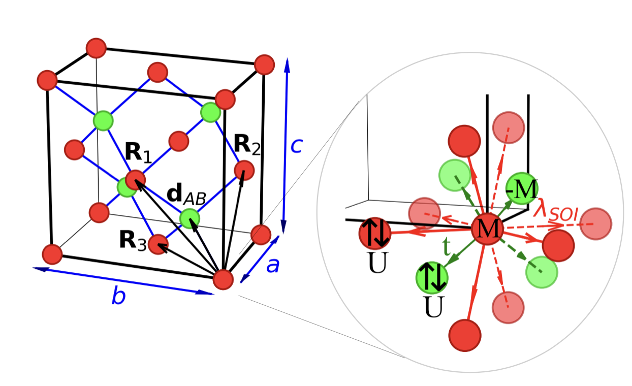
The organic molecular compound, (ET)Ag4(CN)5, is an ideal platform to study the Mott transition on a diamond lattice. The Mott insulator is suppressed under high external pressures of about 10 GPa above which semimetallic behavior has been detected Kiswandhi et al. (2020a). In these compounds, monovalent ET molecules are located at the positions of the orthorhombic diamond lattice shown in Fig. 1. Hence, every ET molecule has four nearest neighbours (n.n.) belonging to the other sublattice that are located at a distance . The ET molecules donate an electron to Ag4(CN)5 anions forming honeycomb lattices surrounding the ET molecules in the planes, leading to half-filled bands. Band structure calculations predict a Dirac nodal line semimetal Shimizu et al. (2019); Kiswandhi et al. (2020a) in contrast to the insulating behavior observed up to 10GPa pressure. This Mott insulator is Néel ordered below K and has a weak ferromagnetic component attributed to the Dzyaloshinskii-Moriya interaction implying a SOI. According to DFT Otsuka et al. (2020), a n.n. hopping, meV, connects the A-B sublattices, while the effective onsite Coulomb repulsion, eV, so that implying a Mott insulator consistent with the low pressure observations. The transition from the Mott insulator to the semimetallic behavior observed at pressures above 10 GPa remains theoretically unexplored.
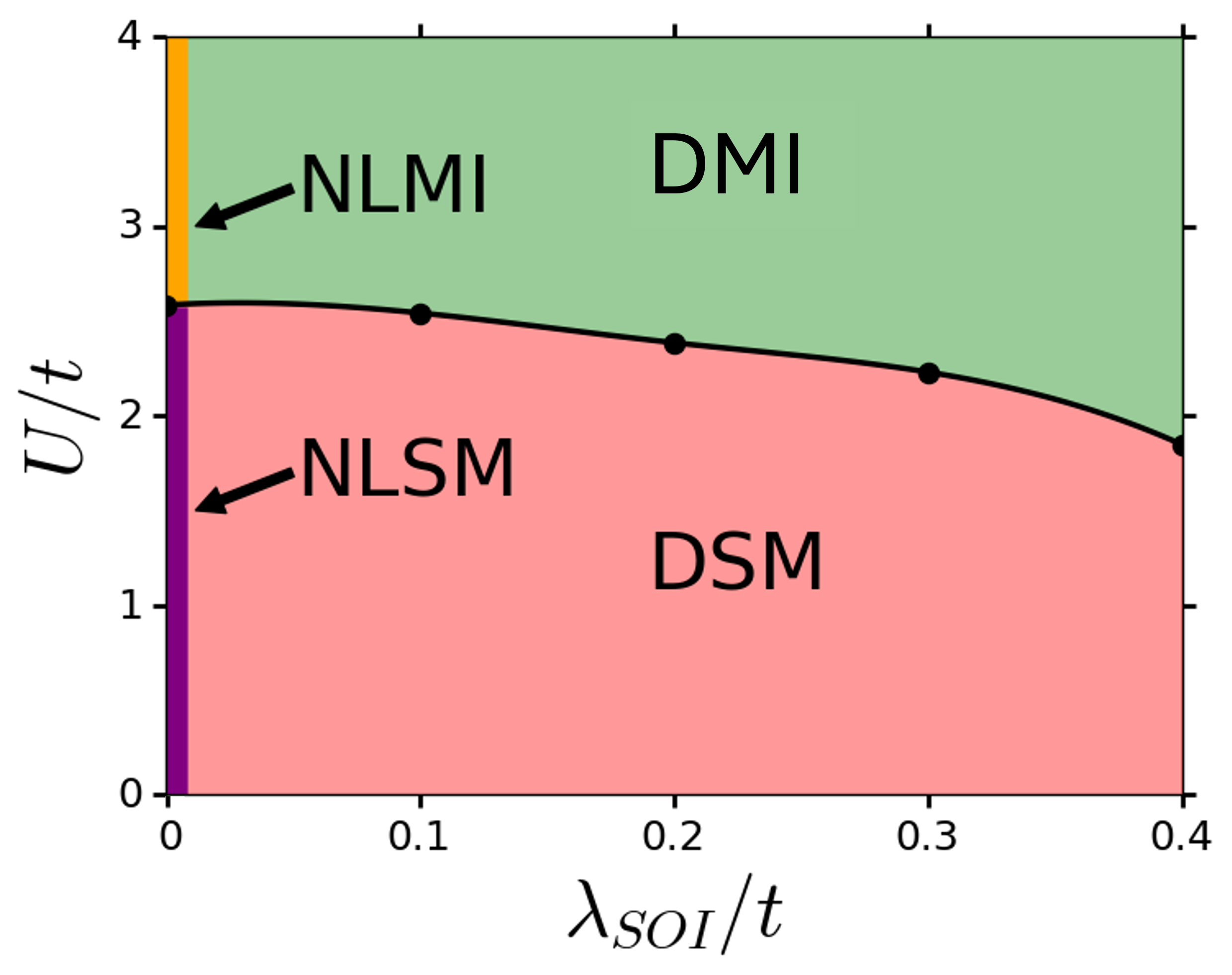
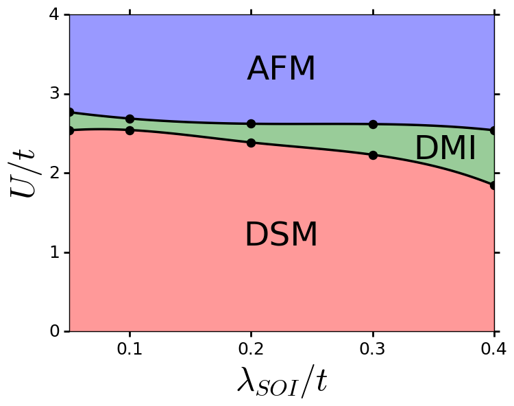
Here, we theoretically explore the Mott transition in (ET)Ag4(CN)5 as a possible platform for TMIs in 3D. Our main results are summarized in the phase diagram of the Hubbard model on an orthorhombic diamond lattice with SOI shown in Fig. 2. For weak Coulomb interactions and no SOI the system is a nodal line semimetal becoming a Dirac semimetal at any finite . A Mott metal-insulator transition occurs at leading to different types of topological Mott insulators depending on the strength of the SOI. While the NLMI at is characterized by having nodal line spinon bands in the bulk, the DMI at hosts Dirac spinons. The slave-rotor approach used in this work leads to Mott insulators in which the spin and charge degrees of freedom are fractionalized. While charge excitations are gapped, spin excitations are gapless. Since the spinons inherit the topological properties of the non-interacting semimetallic phases, the Mott insulator can be regarded a TMI. This picture is corroborated by analyzing the Green’s function across the Mott insulator transition: while the zeros follow the spinon dispersions Wagner et al. (2024) characterizing the topology, the poles describe the Hubbard bands and Mott gap.
The rest of the paper is organized as follows. In Sec. II we introduce a Hubbard model on an orthorhombic diamond lattice to explore the Mott transition. In Sec. III we analyze the various non-interacting semimetallic phases arising in the model depending on the various ingredients such as the SOI or CDW order parameter. In Sec. IV we discuss the strongly interacting limit of the Hubbard model introduced in Sec. II. Sec. V is devoted to the Mott transition and slave rotor mean-field theory. The connection between spinon bands and Green’s function zeros is discussed in Sec. VI. In Sec. VII we discuss our results in the context of experimental observations in (ET)Ag4(CN)5 molecular compounds. In Sec. VIII we summarize our main results and discuss possible extensions of our work beyond slave rotor mean-field theory.
II Hubbard model on orthorhombic diamond lattice
We analyze the Mott transition on the orthorhombic diamond lattice of Fig. 1 based on a generalized Hubbard model extended to include an SOI and an alternating charge density wave (CDW) potential. Thus, the complete model reads:
| (1) |
where:
| (2) |
Since the lattice is bipartite (see Fig. 1), , is the hopping between the two sublattices located in different unit cells whereas, , is the hopping between two sublattices in the same unit cell. If spatial isotropy is broken which could be achieved by applying uniaxial pressure along the direction of the (ET)Ag4(CN)5 compound. We generally take , and as obtained from DFT calculationsShimizu et al. (2019) on (ET)Ag4(CN)5 discussing the anisotropy whenever relevant. is a Fu-Kane-Mele spin-orbit contribution Fu et al. (2007a); Vanderbilt (2018) and an alternating charge density wave (CDW) potential. Here labels the two spin degrees of freedom, is the vector of Pauli matrices acting on spin space. and are bond vectors connecting n.n. sites adding up to bonds between n.n.n. sites on the diamond lattice (see Fig. 1 for the lattice geometry). The SOI term is hermitian, since , and , preserving symmetry. We assume an alternating potential in sublattices A and B, respectively, with in . This term breaks -symmetry but preserves -reversal symmetry. Finally, is a standard onsite Hubbard Coulomb repulsion.
We explore in the following our model (1) in different parameter regimes. As shown below, in the non-interacting limit, we can have a nodal line, a Dirac or a Weyl semimetal depending on and . At strong coupling, the model can be mapped onto a FM model with an AFM Ising interaction in the -direction. The Mott transition at intermediate is explored based on slave rotor mean-field theory (SRMFT).
III Topological semimetals
At , we can neglect and different band structures arise depending on the terms kept in the non-interacting hamiltonian. We first consider three different semimetals with isotropic hoppings, , but different parameters: (i) , (ii) , , (iii) , . We finally consider the possibility of a topological insulator with (iv) and . Case (ii) corresponds to a 3D Fu-Kane-Mele type of modelFu et al. (2007a). We discuss these three cases paying special attention to their associated topological properties.
Nodal line semimetal, . We first consider the simplest non-interacting model, a n. n. tight-binding model on the diamond lattice:
| (3) |
In reciprocal space, the model can be more simply expressed in terms of Pauli matrices as:
| (4) |
where the Pauli matrices are now denoted by with (corresponding to components) and act on the sublattice space (), with:
| (5) |
| (6) |
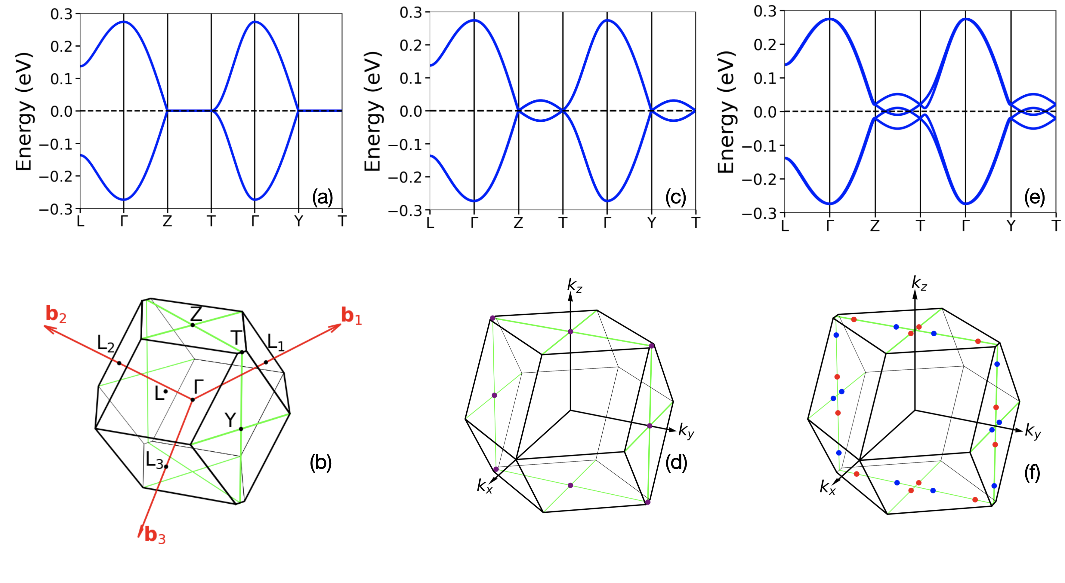
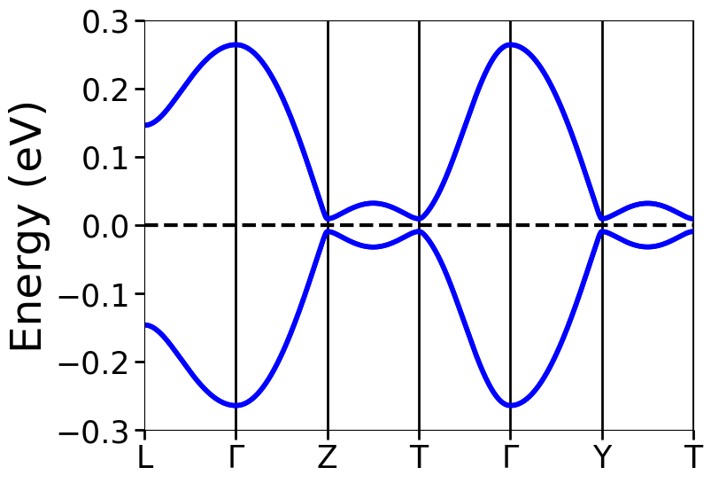
The band structure associated with is shown in Fig. 3 (a) for . It is worth noting the band degeneracies arise along the and segments of the Fermi energy, , of the half-filled system. A simple analysis of (4) shows that the dispersion relation can be expressed as:
| (7) |
so that the band degeneracy at points must satisfy the condition:
| (8) |
at . The dimension of this degeneracy is found to be equal to , with being the dimensionality of the system () and the codimension of the node. This codimension refers to the number of equations a -point has to verify for accommodating a degeneracy which from (8) we can see that . Moreover, a discussion in Bzdušek and Sigrist (2017) shows that in two-band systems the codimension of the nodes is found to be equal to the minimum number of different Pauli matrices necessary for expressing the hamiltonian (3). This arises from the fact that for every Pauli matrix that appears, an equation of the form can be considered as a new condition on the -point to display a band degeneracy. Here, is the coefficient associated with a particular Pauli matrix .
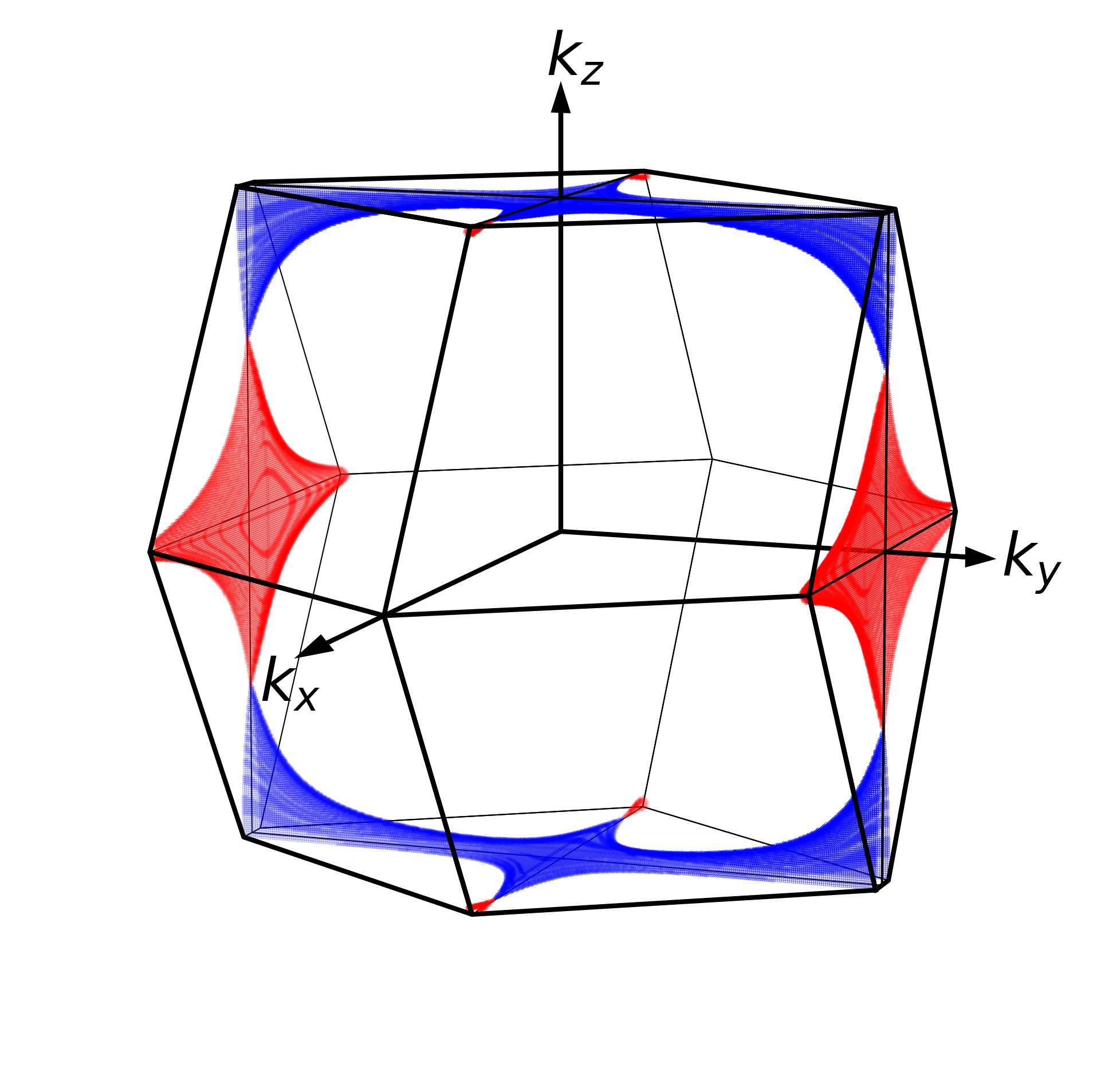
Since band degeneracies must form one-dimensional lines in -space, which are denoted as nodal lines or nodal loops if they are closed. The set of satisfying (8) lead to three closed mutually perpendicular rectangular nodal lines centered at the -point as shown in Fig. 3 (b).
If hopping terms up to four n.n. are considered, the Hamiltonian in reciprocal space would read:
| (9) |
with being the identity matrix. The dispersion relation becomes:
| (10) |
where expressions for , and are given in App. A. Since is not a Pauli matrix, it is irrelevant for determining the node codimension and so remaining also in this case. Although this system is also characterized by the presence of nodal lines the Fermi surface consists of electron and hole pocketsShimizu et al. (2019); Otsuka et al. (2020) (see App. A).
We now consider the topological properties of the NLSM described by a 3D model of the type (3) with codimension, . Due to their codimension, =2, Bzdušek and Sigrist (2017) the only -spheres (spheres of dimension ) that can wrap the nodal loops accommodating a topological charge are those with (loop), 2 (sphere). Hence, nodal loops are characterized by two independent topological indices , which belong to the homotopy group Fang et al. (2015) and give information on the way in which the nodal loops evolve when perturbing the Hamiltonian while preserving its , and SU(2) symmetries.
The topological index is simply the Berry phase over a ring that links with the nodal loop,
| (11) |
where
| (12) |
is the Berry connection and a band index. Since in this case we only have one occupied band, described by the Bloch eigenstate, , with eigenenergy given in (7). This state takes the form:
| (13) |
in our chosen particular gauge. Thus,
| (14) |
As shown in Rui et al. (2018a), a null value of indicates that the degeneracy is accidental and removable by any small perturbation preserving the symmetries of the hamiltonian. On the other hand, a non-zero value of the Berry phase means that the nodal loop is protected by SU(2) and symmetries.
The robustness of the nodal loops against a small perturbation preserving all hamiltonian symmetries can be analyzed by modifying in of (5) with which dimerizes the hoppings along the direction. Note that the present NLSM described by hamiltonian (3) falls in the AIII class according to the classification scheme of Ref. Bzdušek and Sigrist, 2017 (see Table II in this reference).
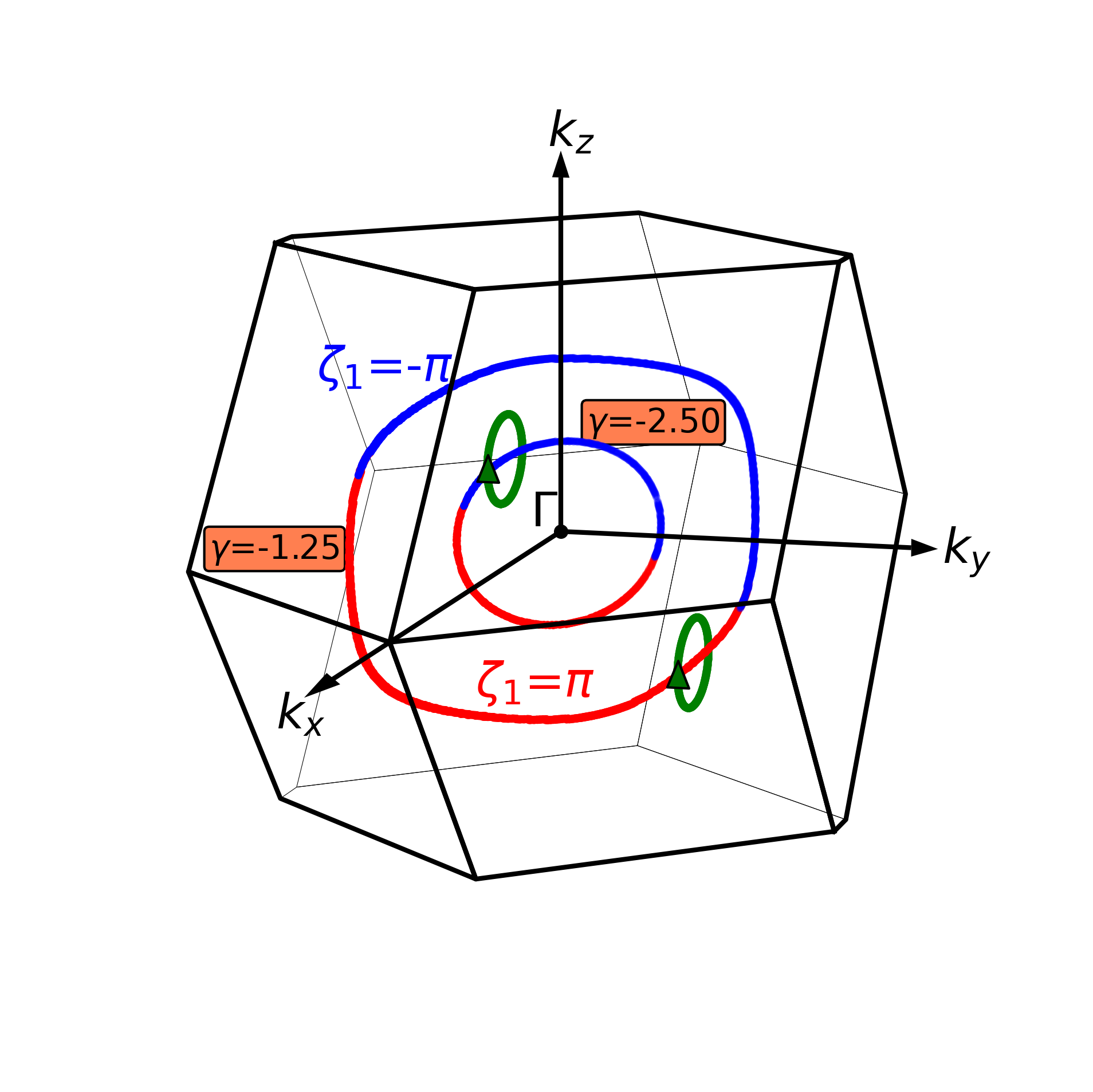
In Fig. 4, the dependence of nodal loops on is shown. As decreases, the nodal loop contracts towards the -point, until the critical is reached, at which the nodal line becomes a single point localized at . For , the nodal loop disappears and the system becomes gapped. A similar situation occurs for (not shown). The only differences are that the TRIM to which the loop contracts is now L, and that the critical value at which the loop disappears is García (2020). The Berry phase, along the nodal loop is obtained from Eq. (11) by integrating over the green interlinked rings shown in Fig. 4. Since half of the nodal line has and the other half has: , the total Berry phase inside the FBZ is zero. Hence, the second topological index of the nodal loop, , indicating that it cannot be considered a charge monopole. This is consistent with the fact that similarly to Weyl nodes (except that Weyl nodes can also have a -charge of -1), charged nodal lines can only be created and annihilated in pairs but cannot shrunk to a point becoming gapped when continuously varying Hamiltonian parameters without breaking the symmetries as happens in our present case for .
In the studied NLSM, the bulk-boundary correspondence guarantees the presence of in-gap states within the projected Surface Brillouin Zone of a system characterized by a nodal loop with quantized Berry phases in its bulk.Chan et al. (2016) These surface states, confined to the projection of the nodal loop onto the surface, exhibit a nearly flat dispersion reminiscent of a drumhead, hence the term "drumhead states". This flat dispersion results in an exceptionally high density of states and significant correlation effects,Burkov et al. (2011) positioning these systems as promising platforms for exotic electronic phenomena, such as high-temperature superconductivityKopnin et al. (2011) and the emergence of Majorana fermions.Chen et al. (2021b) Beyond theoretical interest, experimental studies of these systems have accelerated in recent years, notably with the detection of drumhead surface states in nodal-line semimetallic materials via ARPES techniques.Muechler et al. (2020); Hosen et al. (2020)
In summary, the nodal lines of the NLSM occurring for have non-zero Berry phases along the nodal line but are uncharged, . These type of nodal lines are one-dimensional analogues of Dirac nodes so they are more specifically denoted Dirac nodal lines.
Dirac semimetal: , . We now consider our non-interacting model which includes SOI effects on the NLSM:
Since SU(2) symmetry is broken, , is no longer but . Therefore, cannot be expressed through Pauli matrices but rather in terms of tensor products among them:
| (16) |
with and . Pauli matrices acts in the lattice subspace whereas Pauli matrices acts on the spin subspace . The different tensor products between Pauli matrices give rise to 16 Dirac matrices, .
Our Hamiltonian preserves space-time reversal symmetry, i.e. with , thus it can be expanded in terms of matrices that commute with . We will search for these among the 16 Dirac matrices. Since the inversion operator swaps , while leaving spin unchanged, it can be represented as . The time-reversal operator for spin-1/2 particles is represented as in the convention of a rotation around the spin -axis, with indicating complex conjugation. Both symmetry operations also reverse when acting on functions of such variable, therefore, their composition is evidently the identity over -space. Thereby, and , where the commutation of a generic element with this operator is reduced to the condition . From the 16 different Dirac matrices only 6 of them fulfill the previous condition, the so called -even Dirac matrices:
| (17) |
Thus, the Hamiltonian can be expressed in the reciprocal space in terms solely of these 6 matrices. In this way, we have managed to reduce the dimension of the representation from 16 to 6, which in fact are actually 5 matrices, since does not contribute up to the n.n. hoppings:
| (18) |
The different associated to this Hamiltonian can be seen in App. B.
Similarly to the two-band case, the dispersion relation of this Hamiltonian reads:
| (19) |
Under the presence of symmetry, Kramers degeneracy always enforces a two-fold spin degeneracy. This is why, despite our hamiltonian being , the band structure consists of only two bands which are two-fold degenerate.
As stated above, the node codimension is equal to the minimum number of Dirac matrices needed for expressing the hamiltonian. Therefore, , and a four-fold degeneracy should be ruled out under the effect of this hamiltonian. This is true for all the different points of -space, except for those belonging to the TRIM. Recalling that , we have that
| (20) |
where we have taken advantage of the fact that Dirac matrices satisfy (Euclidean Clifford algebra). Since at a TRIM , we must have:
| (21) |
for any function . Therefore, the codimension at a TRIM reduces to , since it only has to verify the equation for accommodating a four-fold degeneracy. This makes TRIM points very prone to hosting degeneracies among all bands in these systems.
The band structure associated to the SOI Hamiltonian (LABEL:eq:Dirac_H) is shown in Fig. 3 (c). Apart from the two-fold spin degeneracy found throughout the entire -space, the band structure features four-fold degeneracies at the TRIM points , , and . Notice that since the TRIM are the only points in reciprocal space at which , the four-fold degeneracies appear as disconnected points despite (surface) as shown in Fig. 3. Since the dispersion at these four-fold degenerate points is linear they can be regarded as Dirac cones characterizing a Dirac semimetal.
Weyl semimetal: , . We consider the effect of a CDW potential on the DSM through the model:
| (22) |
The CDW term leaves the spin subspace intact but acts with opposite signs on () or () sublattices. Based on this, it is straightforward to see how the Dirac matrix associated to is . Therefore, our new Hamiltonian in the Dirac matrix representation reads:
| (23) |
which is readily diagonalized leading to four bands:
| (24) |
Here, the superindices and denote valence and conduction bands, respectively. Hence, by breaking the symmetry, we have lifted Kramer’s degeneracy present at . Still many degeneracies can occur among pairs of bands at specific -points of the FBZ. Despite this we focus on the degeneracies occurring at the Fermi level, , since these characterize the low energy electronic properties of the system. From (24) it is easy to see that a degeneracy with can only occur between and . The set of -points at which band degeneracies occur are defined by the conditions:
| (25) |
where the codimension of the band degeneracy is leading to Weyl nodes in the 3D -space.
Weyl nodes are characterized by their -charge or chirality: with a spherical surface wrapping the Weyl node, is the Berry curvature and the Chern number. The computation of can be greatly simplified by noting that the Weyl nodes can be described through a hamiltonian:
| (26) |
as they only involve two bands: and . Following Vanderbilt (2018); Goikoetxea et al. (2020) the chiralities of the Weyl nodes described by by a hamiltonian of the form can be expressed as:
| (27) |
with , the determinant of the Jacobian matrix evaluated at the Weyl point located at .
As is increased each Dirac cone at the , and TRIM points split into two Weyl nodes of opposite chiralities, , as it should. The band structure at is shown in Fig. 3 (e) which hosts the 24 Weyl nodes shown in Fig. 3 (f). As expected from the Nielsen-Ninomiya “fermion doubling” theoremNielsen and Ninomiya (1983), Weyl nodes occur in pairs of opposite chiralities so the system has zero net chirality. At a critical , Weyl nodes of opposite annihilate finally becoming a trivial band insulator at larger .
Topological insulator: . Finally, we consider the possibility of stabilizing, at weak coupling, a topological insulator induced by SOI. As discussed above, model (LABEL:eq:Dirac_H) leads to Dirac cones in the band structure. By introducing a distortion in the bonds by taking , in the presence of we can open a gap in the system leading to a topological insulator as shown in 5. The topology of an insulator where symmetry is preserved is described by four independent indices Fu et al. (2007b), usually displayed as which can take odd and even values (). They are divided between strong () and weak () indices, with the strong one being the most important. An insulator with an odd value of is classified as a strong topological insulator (STI), meanwhile if it presents an even value of it is said to either be a weak topological insulator (WTI) or to be topologically trivial. The difference between weak and trivial topology is given by the three weak indices. An insulator with an even but at least one odd is said to be topologically weak whereas an insulator described by the index set () is topologically trivial.
If, in addition to being -symmetric, a system presents symmetry, like in the present case, the computation of these indices is greatly simplified since they depend only on the parity of each pair of Kramers degenerate occupied bands at the eight TRIM in the FBZ Fu and Kane (2007). These special points can be expressed in terms of the primitive reciprocal lattice vectors as . As in the Fu-Kane-Mele model there is a single pair of Kramer degenerate occupied bands, these topological indices can be expressed as:
| (28) |
| (29) |
where is the eigenvalue associated to the parity operator when measured over the pair of Kramer degenerate occupied bands at a TRIM. Note that the four points describing each index all lay on the same plane. Moreover, in the same notation used previously for the TRIM, the weak indices read:
| (30) |
In the present model we have and at the TRIM the Hamiltonian reduces to . Thus, the Bloch eigenstates of the Hamiltonian are also eigenstates of at the TRIM. Since and , the eigenvalues associated with are . Therefore, the TRIM points have a definite parity given by the eigenvalues of . From a simple derivation, shown in App. C, one arrives to the following expression for the parity of the Kramers degenerate occupied bands at the TRIM:
| (31) |
This definition, we find that at and at , while being at . Furthermore, we find that at the points , and the parity is for the distorted Hamiltonian. Combining all these results we arrive at the expression for the set of indices:
| (32) |
Hence, if the distorted bond is stronger than the other three, meaning that our system is dimerized, we find that we have a strong topological insulator, meanwhile if the bond is weaker than the other three, implying that our system is layered, we find that it is a weak topological insulator. These results imply that any distortion in the bond transforms our Dirac semimetal into an insulator which can be either topologically strong or weak but never topologically trivial.
IV Effective spin model in the strongly interacting limit
We now analyze our model (1) in the limit. In this case, the model can be mapped onto a Heisenberg-type model: on a diamond lattice which reads:
| (33) |
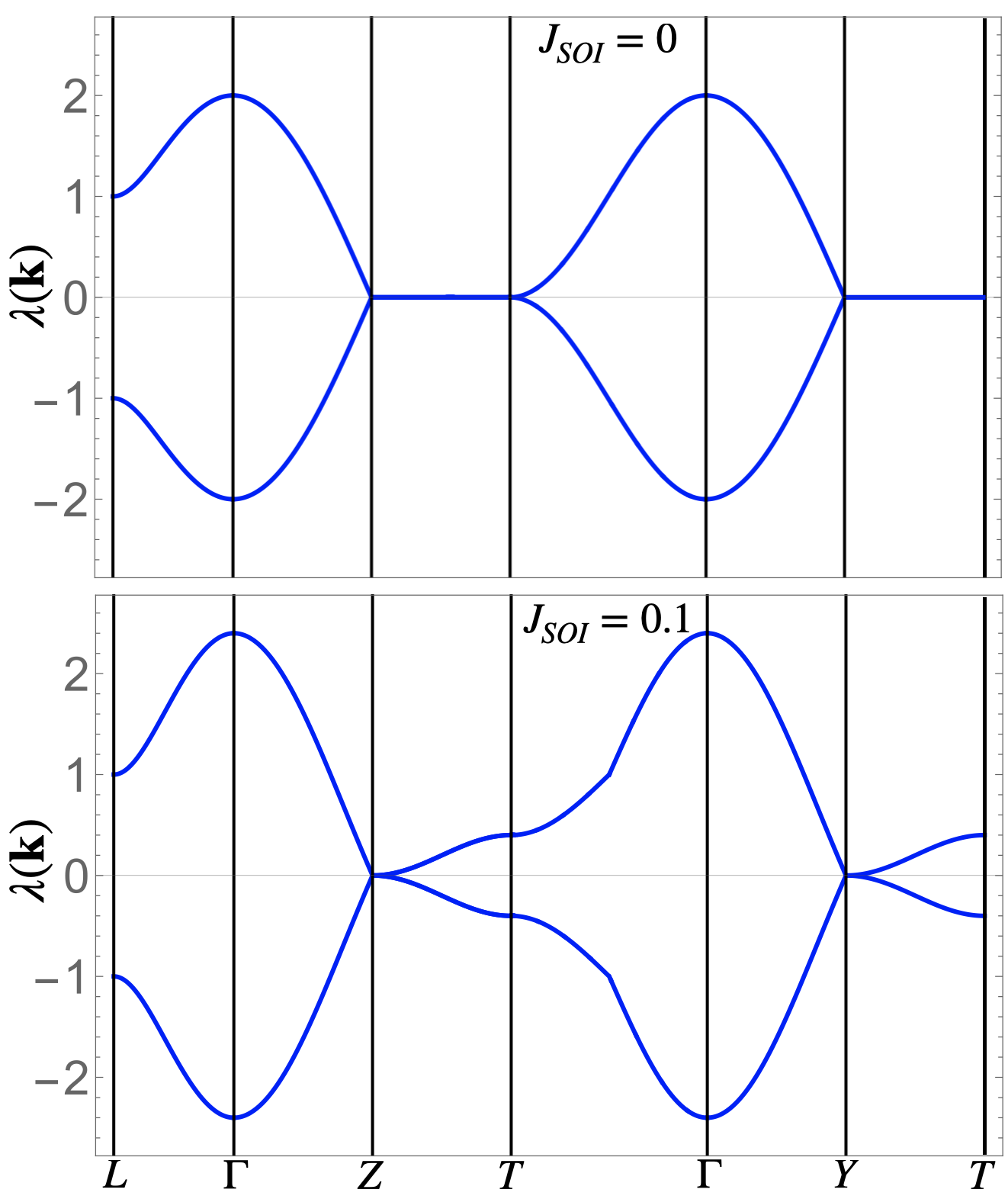
where is the standard n.n. AF Heisenberg coupling and a n.n.n. coupling induced by the spin-orbit coupling. This spin model consists of a FM XY-term and an AFM Z-term which favors antiparallel alignment of the spins similar to the spin model found in Mott insulators in the honeycomb latticesRachel and Le Hur (2010). Note that in the present model we have neglected a possible n.n.n. Heisenberg coupling, since in the actual (ET)Ag4(CN)5 molecular compound. Indeed, the ground state of the Heisenberg model on the diamond lattice is Néel ordered for and magnetically disordered for . Hence, we only consider the n.n. and the n.n.n. but neglect .
Using the Luttinger-Tisza semiclassical approachLuttinger and Tisza (1946); Luttinger (1951); Litvin (1974) we analyze the magnetic ground states of model (33). The main result as discussed in App. D is that the Néel order which can be pointing in any direction when occurs in the plane when . Hence, although Néel order is expected in the presence of SOI, the spins must lie within the plane for .
V Mott transition: slave rotor mean-field theory
Since an exact solution of model (1) particularly at intermediate is very challenging approximations are required. Slave-rotor mean-field theory (SRMFT)Florens and Georges (2002); Fernández López and Merino (2022); López et al. (2024) allows for a numerically efficient description of the Mott metal-insulator transition. It captures the bandwidth reduction with increasing and is consistent with more sophisticated approaches like Gutzwiller-type wavefunctions, DMFT and variational cluster approaches.Florens and Georges (2004)
V.1 Slave-rotor mean-field theory
In the slave-rotor approach, the electron creation (annihilation) operator is splitted into a spinless bosonic field carrying only charge (rotor) , and a neutral fermion carrying only spin (spinon), :
| (34) |
Thereby, model (1) with , expressed in the slave-rotor formulation reads:
where is the orbital angular momentum that describes the charge quantum number linked to site and acting as a lowering operator of .
Thus, the slave-rotor electron decomposition in spinons and rotors transforms the kinetic energy from a quadratic to a quartic contribution. Hence, a Hubbard-Stratonovich mean-field approximation is performed to factorize these terms:
| (35) |
where we take and . If one further consider the mean-field ansatz, , the hamiltonian can be naturally splitted into a spinon and a rotor hamiltonian, , with:López (2024)
| (36) | ||||
| (37) |
where and for n.n. (n.n.n.).
Under the SRMFT approach, the original model has been mapped onto a free fermion model (renormalized by interactions) coupled to a quantum -model for the rotor variables . Different approaches with different levels of approximation can be used to solve . At the strict local level, since , Florens and Georges (2002, 2004) a trivial paramagnetic Mott insulator consistent with the DMFT prediction survives. Here we take into account short-range spatial electronic correlations by using the soft boson representation Florens and Georges (2004) by which , imposing the constraint, , on average. Such SRMFT approach captures intersite electronic correlations present in cluster DMFT Liebsch (2011); Wu et al. (2010); Wang et al. (2017) which have been shown to play a crucial role in the Mott transition in semimetals.López et al. (2024) In this approach, the spinons in the Mott insulator, , disperse since , and form a Fermi surface consisting of the nodal lines/points in the case of the semimetals considered in the present workSong et al. (2023). Hence, our Mott insulator is effectively fractionalized into gapped charge excitations and gapless spinons forming a U(1) Dirac QSLMaciejko and Fiete (2015).
Based on the approach described above our hamiltonian (1) in the SRMFT approach reads:
| (38) |
with:
| (39) | ||||
| (40) |
where is the Lagrange multiplier introduced to impose the constraint, , and the renormalization factors read:
with, for n.n. (n.n.n.), the spinon and rotor renormalization factors. Therefore, the slave-rotor approach allows us to explore the behavior of spin-only (spinons) and charge-only (rotors) quasiparticles into which electronic excitations have fractionalized.
From the above, the spinon hamiltonian, , and the kinetic energy contribution to the rotor hamiltonian, read:
| (41) | ||||
| (42) |
with:
| (43) |
where the are the -even Dirac matrices. These expressions reduce to:
| (44) | ||||
| (45) |
when . Moreover, since our rotor Hamiltonian has 2 bands, a rescaling of is performed in order to recover the correct atomic limit Fernández López and Merino (2022).
We can now introduce the finite Green functions for the spinons and rotors from their corresponding decoupled hamiltonians (39) and (40):
| (46) | ||||
| (47) |
where and , with , are the fermionic and bosonic Matsubara frequencies, respectively. and are the dispersion relations of the spinons and rotors and a band index. Note that these dispersion relations contain renormalization effects since they are associated with the kinetic energy contributions to and which explicitly depend on and . The derivation of and is provided in App. E.
As shown in App. F, the renormalization factors, and can be expressed as:
| (48) | ||||
| (49) |
where is a vector connecting sites and of the lattice, and and are the eigenvectors associated to the kinetic parts of the rotor and spinon Hamiltonians, respectively. Moreover, here and represent the Fermi-Dirac and Bose-Einstein distributions and .
Similarly, the constraint can be expressed (see App. F for details) as:
| (50) |
where is the number of sites in the unit cell.
We have thus obtained a set of three self-consistent equations, (48), (49) and (50), from which we compute , and for given and .
The bosonic nature of the rotors implies the possibility that they can form Bose-Einstein condensates. Within SRMFT approach, the electron quasiparticle weight, , is directly related with the rotor fraction condensing Florens and Georges (2004) at (at which the minimum in occurs). Isolating the -mode in (48) and (50), we write:
| (51) | ||||
| (52) |
where has become a new parameter computable from the self-consistent equations.
These equations are iteratively solved as follows. We start with an initial guess for , and , for which we diagonalize the rotor kinetic Hamiltonian and obtain its eigenvectors and eigenvalues . From them we recalculate from the constraint equation (52), before using it to evaluate, in the same equation, the sum over in order to obtain a new value for . With the knowledge of the new and we recalculate the spinon renormalization factor , using (51). We then diagonalize and obtain the eigenvalues and eigenvectors of the spinon kinetic Hamiltonian, which we use for recalculating a new value of through (49). If the recalculated values of , and are identical to the initial ones, convergence has been achieved and these are the true self-consistent parameters of our system at a given and . Otherwise, the process is repeated, reinjecting the recalculated parameters at the beginning of the procedure. The process is repeated until full convergence is achieved.
At self-consistency, physical properties such as the rotor gap, can be computed Florens and Georges (2004). A non-zero indicates a bulk charge gap in the systems, , Mott insulator.
V.2 Quantum spin liquid Mott insulator
Hence, within SRMFT we can encounter two different phases. A semimetallic phase at weak , adiabatically connected to the non-interacting semimetal, characterized by and no charge gap , and at large- a nonmagnetic insulating phase characterized by and non-zero charge gap, , i.e. a quantum spin liquid Mott insulator.
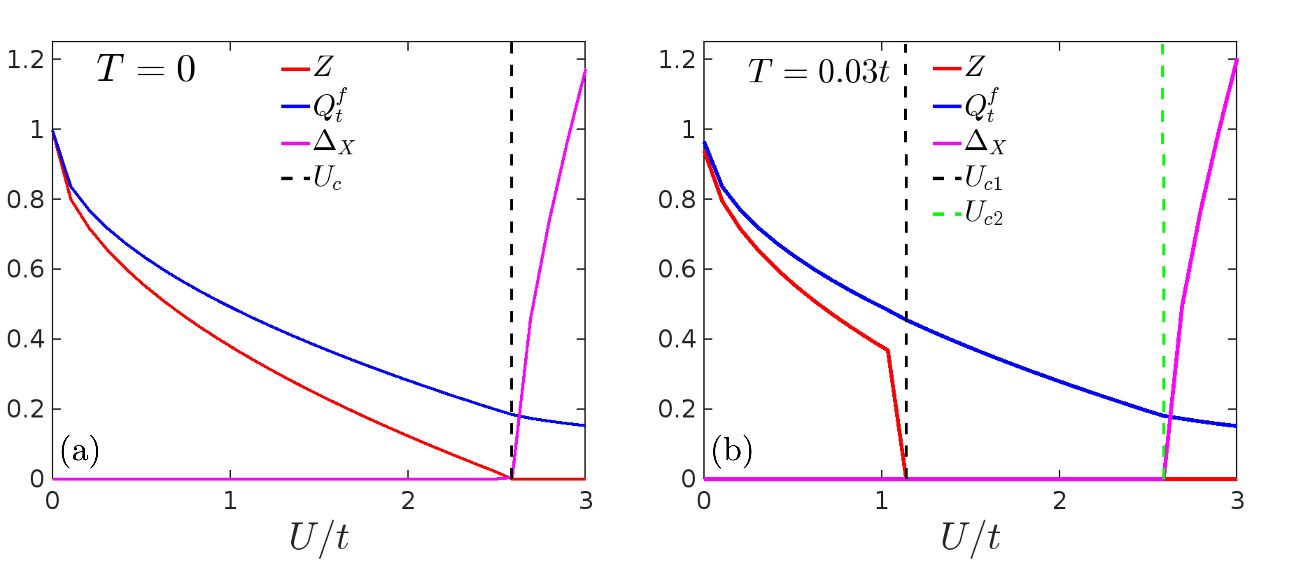
Fig. 6 (a) shows the dependence on of , and for the Hubbard model on a diamond lattice (1) with no SOI. We can see how the quasiparticle weight vanishes, , concomitantly with the charge gap opening, , at the critical value of . Therefore, the two mentioned phases can be clearly distinguished here at . The nodal loop semimetallic phase ( and ) for and the Mott insulating phase ( and ) for values of . In the limit , thus recovering the expected non-interacting nodal loop semimetal.
In Fig. 6 (b) the dependence of the SRMFT parameters at finite temperature, , is shown. In contrast , at finite- the transition from the nodal loop semimetal to the Mott insulator becomes a two-step process, with the quasiparticle weight abruptly vanishing at whereas the charge gap opens up at . Hence, a new phase is found at between and , characterized by and corresponding to a bad smiemetallic phaseFernández López and Merino (2022); López et al. (2024). Interestingly, in this phase and , implying that spinons retain the NLSM dispersion of the nearby semimetallic phase. Thus, this phase can be identified as a bad nodal loop semimetal (BNLSM).
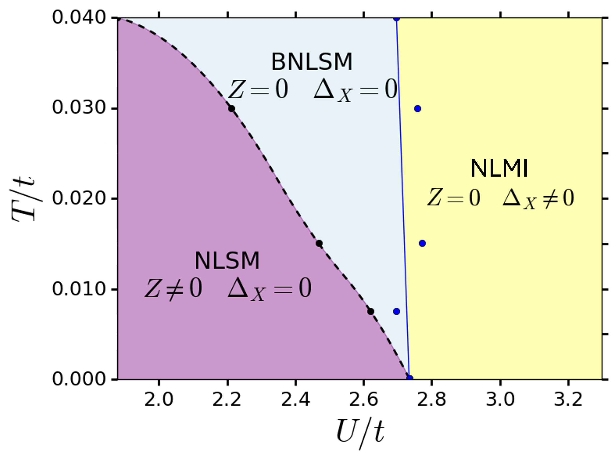
The phase diagram obtained from SRMFT is shown in Fig. 7. While the rotor gap opens up at nearly independently of , the quasiparticle weight vanishes, at a lower which increases with increasing . Hence, the bad semimetallic phase is stabilized in a broader range with increasing . This is consistent with the fact that the sudden drop found in at finite- is due to thermal fluctuations. Since at higher , thermal fluctuations are enhanced, the drop in occurs sooner.
V.3 Magnetically ordered Mott insulator
Since the orthorhombic diamond lattice is bipartite we can expect Néel type of magnetic order to occur. We explore magnetically ordered phases with our slave rotor approachKo and Lee (2011); Yang and Liu (2024) by introducing a magnetic order parameter in our model. For Néel order we introduce the staggered magnetization:
| (53) |
Thus, this parameter describes staggered magnetic order with alternating from positive to negative when going from A to B sites. Thus, indicates Néel order sets in the lattice.
Since involves spin degrees of freedom only, it affects the spinon part of the slave rotor mean-field hamiltonian.Yang and Liu (2024) Hence, the hamiltonian is modified as:
| (54) |
where:
| (55) |
apart from some irrelevant constants. In reciprocal space, this new term reads:
| (56) |
Taking into account introduces a new self-consistent equation which must be added to our previous original SRMFT equations. By transforming (53) to the reciprocal space and performing the corresponding Matsubara sums, the new equation for is of the form:
| (57) |
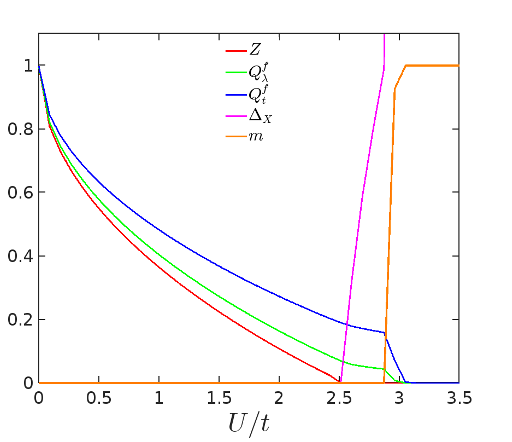
In Fig. 8 we show the dependence of the SRMFT parameters including with at for fixed . An AFM state emerges within the DMI phase i.e. for , with the magnetic moment reaching the fully saturated AFM Néel ordered state very rapidly. Still, before reaching full saturation, a region with and non-zero arises indicating coexistence of AF and QSL.
We have obtained a complete vs. phase diagram including AFM order as shown in Fig. 9. Crucially, the DMI spin disordered phase survives in an intermediate range between the DSM and AFM phases in a broad range of explored. As in the phase diagram of Fig. 2, we find that displays a smooth decay with . This is related to the redistribution of non-interacting density of states towards higher energies with as explained in App. G.
The (ET)Ag4(CN)5 compounds display a Mott insulating phase with AFM order at low and pressures up to around 8 GPa. Above 12 GPa resistivity measurements are consistent with semimetallic behavior. Interestingly, an intermediate phase in the pressure range 8-12 GPa has been interpreted as a disordered Mott insulator Kiswandhi et al. (2020a). From our analysis, we can interpret such intermediate phase observed in terms of the DMI found. Further experiments probing magnetism at high pressures are needed to check the nature of the intermediate phase.
VI Topology from Green’s function zeros
It has been recently shown in an exactly solvable quantum many-body model that the topological properties of a Mott insulator can be obtained from the Green’s function zeros Bollmann et al. (2024). Interestingly, within a slave-rotor approach to the Kane-Mele Hubbard model the Green’s function zeros have been found to follow the underlying spinon dispersionWagner et al. (2024). Thus, we characterize the Mott transition on the diamond lattice based on such Green’s function zeros perspective. For illustrative purposes, we compare the behavior of the Green’s function zeros with the poles determining the spectra density, , across the transition. In other words, we monitor the topological character of a NLSM as the Coulomb interaction is increased across the Mott transition solely based on the electronic Green’s function.
We first need to obtain the non-local electron Green’s function from the convolution of the spinon and rotor Green’s functions:Wagner et al. (2024); He and Lee (2022, 2023)
| (58) |
where and () are the fermionic (bosonic) Matsubara frequencies. Note that the Green’s function is a matrix. The details on the derivation of the electron Green’s functions are given in App. H.
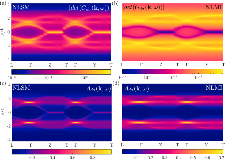
The absolute value of the determinant is compared with the spectral density, along FBZ symmetry directions in Fig. 10 both in the NLSM and NLMI phases. Since in the NLSM, , spinons and rotors are combined forming electron quasiparticles leading to poles in the Green’s function which dominate the spectra of both (Fig. 10 (a)) and (Fig. 10 (c)). Apart from the coherent quasiparticle contribution, one can appreciate the incoherent Hubbard bands arising from the convoluted rotor-spinon excitations.
In contrast, in the NLMI, strong electronic correlations suppress the quasiparticle weight to zero, , leading to electron fractionalization. The electron fractionalizes into gapless neutral spinons and gapped charged rotors. This is reflected in (Fig. 10 (b)) and (Fig. 10 (d)). While the and spectra are dominated by the Hubbard bands, the zeros of inside the Mott gap disperse as the spinon nodal lines characterizing the Fermi surface of the NLSM. Thus, the fractionalized NLMI phase is characterized by the occurrence of gapless Green’s function zeros inside the Mott gap. Since nodal lines characterize the topology of the NLSM, one can automatically associate the topological properties of the NLMI with the zeros of the Green’s function. These in turn are found to trace the spinon nodal lines obtained within the slave-rotor approach.
In the NLSM phase, topological drumhead surface states are expected to occur at the projected surface Brillouin zone following the bulk-surface correspondence. These are analogous to the Fermi arcs arising at the surface of Weyl semimetals. Based on the bulk-surface correspondence established in the strongly interacting regimeWagner et al. (2023); Blason and Fabrizio (2023), the NLMI should host gapless boundary zeros in the Green’s function. Since within slave-rotor theory, the Green’s function zeros are directly connected to the gapless boundary spinons, we can conclude that the NLMI hosts drumhead surface states of spinons. These drumhead surface states differ fundamentally from the metal surface states, which are characterized by poles of the Green’s function. The replacement of poles by zeros illustrates how fractionalization reshapes both bulk and boundary physics, emphasizing the purely spin-driven topology of the NLMI phase. Moreover, intriguing phenomena at NLMI/NLSM interfaces can be expected within slave-rotor theoryWagner et al. (2024). The gapless boundary spinon modes manifesting as Green’s function zeros would cancel the spinon contribution to the NLSM’s surface states leaving only drumheads of holons propagating at the NLMI/NLSM interface.
Our analysis reinforces the relevance of the single particle Green’s function, , as a diagnostic tool of the topological properties across the NLSM to NLMI transitionWagner et al. (2023); Bollmann et al. (2024); Wagner et al. (2024). While in the NLSM, conventional quasiparticles are described by the poles as expected, in the NLMI the zeros of determine the topological properties of the strongly interacting NLMI.
VII Comparison with observations in (ET)Ag4(CN)5 compounds
Experimental observations show how (ET)Ag4(CN)5 compounds are Mott insulators up to hydrostatic pressures of about 3 GPa. The first important issue is whether a metallic state is induced at larger pressures due to the further increase in the bandwidth. Band theory predicts that such metallic state is actually a NLSM. Shubnikov-de Haas and de Haas-van Alphen oscillations may be used to extract the Fermi surface shape and confirm or not their existenceMüller et al. (2020). The Dirac nodal lines could also be probed through ARPES experiments. Characteristic drumhead surface states extending over the area enclosed by the nodal lines arise at the surface Brillouin smoothly connecting to the bulk band crossings. Under an applied electric field topological transverse currents perpendicular to the applied field associated with opposite Berry phases on the nodal loop emerge. However, since the contributions on opposite sides of the nodal loop cancel there is no net induced current unless a filtering device is usedRui et al. (2018b).
Based on our SRMFT approach, (ET)Ag4(CN)5 is a Mott insulator that hosts topological features. Due to spin-charge separation, the charge-only excitations are gapped while spinons form spinon nodal lines. Since spinons are neutral particles they are difficult to detect but thermal instead of charge conductivity experiments could be used to probe the nodal lines. On the other hand spinon drumhead surface states are expected to occur in the Mott insulator within our SRMFT approach. They are predicted to lead to a suppression of the bulk Mott gap in ARPES experiment probing surface layers onto which the nodal loop can be projected. In the present case and based on Fig. 3(a), the drumhead surface states will arise on the - and - surface BZ planes. By adsorbing a magnetic impurity in the surface of (ET)Ag4(CN)5 a spinon Kondo-effect can occur in which the magnetic impurity forms a singlet with the spinons of the gapless QSLsHe and Lee (2022). This in turn would lead to features in the differential conductance measured in STM experiments probing the tunneling currents through the surface states modified by the presence of the magnetic impurity. Finally, the magnetic order in our TMI would be of the Néel type always as shown in Fig. 7. We can expect the Néel ordered spins to lay within their plane under SOI.
We now discuss our results in the light of recent experiments on (ET)Ag4(CN)5 at higher pressures reaching 14 GPa Kiswandhi et al. (2020a). By increasing the pressure the electron-electron interaction is effectively reduced. The power law dependence of the resistivity detected at low at high pressures with decreasing from 2.6 to 1.78 as the pressure is increased from 8 GPa to 10 GPa. This can indicate the proximity of the Mott insulator to a transition to a semimetal. This would be consistent with the three possible semimetallic states discussed: a NLSM, a DSM or a Weyl semimetal. However, although SOI is expected to be small in (ET)Ag4(CN)5 crystals it may be sufficient to open a small gap leading to the topological insulator introduced previously. All four weakly interacting phases discussed would have specific edge states related to their topology. The NLSM would host drumhead surface states, the DSM flat surface states connecting the Dirac cones, the WSM Fermi arcs and the topological insulator Z2 surface states which may be distinguished through ARPES and/or STM experiments.
The topological Mott insulators found in our work are characterized by having spinon surface states that are in a one-to-one correspondence with the surface states of the topological electron surface states of the weakly interacting phases. Such spinon surface states could lead to a closing of the expected bulk gap at certain surfaces of the Mott insulators which could be searched for in ARPES and STM experiments on the TMIs. Alternatively, as recently shown in Wagner et al. (2024), indirect detection of these spinon topological states can be achieved at the interface between a conventional topological insulator and a TMI. At the NLSM/NLMI interface, the annihilation of the Green’s function zero boundary states with the spin part of the electronic states in the semimetal would result in emergent charge-only (holon) drumhead states. In contrast to spinon surface states, these holon drumhead states could be detected in conventional charge transport experiments.
VIII Conclusions and outlook
We have presented a thorough discussion of the Mott transition in orthorhombic diamond lattices as a platform to access the Mott transition under pressure observed in the molecular compound, (ET)Ag4(CN)5. Our slave rotor analysis predicts a QSL with a charge gap hosting nodal lines (Dirac nodes) of spinons, the NLMI (DMI) for ( ). These Mott insulating phases are topologically non-trivial since they inherit the topological properties of the nearby weakly interacting semimetallic phases through the spinon bands. We confirm this picture by obtaining the Green’s function zeros which are related to the topological properties of the strongly interacting phases Wagner et al. (2023, 2024). Since Green’s function zeros follow the spinon dispersions, experimental probes of spinons are desirable in order to establish the topological properties of the Mott insulators found here. ARPES experiments should detect a suppression of the bulk gap at the surface of these Mott insulators due to the spinon surface bands López et al. (2024). This highlights the crucial role played by Green’s function zeros in accessing the topological properties of strongly interacting systems in general.
Magnetic order is explored based on an extension of the slave-rotor approach. Although Néel order is stabilized in a broad parameter range of the - phase diagram, a DMI phase survives in an intermediate parameter regime between the DSM and AFM Mott phases. Coexistence of QSL and AFM in the Mott insulator is possible in a rather small parameter range before the magnetic order has reached the fully saturated Néel state.
Our results are broadly consistent with recent observations in (ET)Ag4(CN)5 which indicate a transition from an ambient pressure Néel ordered Mott insulator to a semimetallic/semiconducting phase under high pressures. There are indications of an intermediate insulating-like phase which may be interpreted in terms of our DMI phase arising between the AF Mott insulator and the DSM. Depending on SOI, , and degree of dimerization, , different semimetals at high pressures are possible. Even a topological insulator can be favored under sufficient uniaxial pressure along the direction.
Since our work is based on a mean-field approach, future theoretical work should consider electronic correlation effects through numerical approaches. An important question is whether the intermediate QSL Mott insulator survives beyond mean-field theory. Future experiments on (ET)Ag4(CN)5 materials should focus on characterizing the intermediate phase arising at pressures around the Mott transition and analyzing the strongly correlated semimetallic phases arising at larger pressures. The topological aspects of these semimetals could be explored based on magnetic oscillation experiments which can display evidence of non-zero Berry phases associated with the presence of Dirac or line nodes. It is also worth investigating the possibility of inducing superconductivity at even larger pressures.
Acknowledgements.
We acknowledge financial support from (Grant No. PID2022-139995NB-I00) MICIN/FEDER, Unión Europea, from the María de Maeztu Programme for Units of Excellence in R&D (Grant No. CEX2023-001316-M). J. C. acknowledges financial support from the FPI Grant No. PREX2023-000114.Appendix A Tight-binding model for (ET)Ag4(CN)5 up to fourth n.n. sites
For completeness and in order to make our paper self-contained we include the extension of the tight-binding model of the main text up to fourth n. n. sites following previous worksShimizu et al. (2019). The orthorhombic diamond lattice structure shown in Fig. 1 of (ET)Ag4(CN)5 crystals belong to the non-symmorphic Fddd space and point group: , with the center of the lattice being its invariant point. In our work, we have considered the simplest tight-binding model for (ET)Ag4(CN)5 crystals including n.n. hoppings between ET-molecules only. However, in actual (ET)Ag4(CN)5 crystals further distant hoppings are relevant. Table 1 presents hoppings up to the 4 n.n. that an element belonging to the sublattice A of the Fddd diamond orthorhombic lattice and located at the origin has. The intensity of the different hoppings is also presented. All the data were collected from Kiswandhi et al. (2020b). Here an x-ray diffraction experiment was conducted to obtain the geometry of the salt while fittings of tight-binding parameters to first-principles calculations where performed to obtain the hoppings intensities. For reproducing the preliminary results shown in that work, we found necessary to exchange the provided values for and and change the sign given for .
| Order | ( coordinates | Distance (Å) | Hopping (meV) |
|---|---|---|---|
| 1 | |||
| 1 | |||
| 1 | |||
| 1 | |||
| 2 | |||
| 2 | |||
| 2 | |||
| 2 | |||
| 3 | |||
| 3 | |||
| 3 | |||
| 3 | |||
| 4 | |||
| 4 | |||
| 4 |
The tight-binding Hamiltonian with real hoppings (no spin dependence) up to 4 n.n. reads:
| (59) |
where:
| (60) |
| (61) |
| (62) |
Recall that is the identity matrix and are the Pauli matrices. In contrast to the n.n. tight-binding model in which the Fermi surface consists of Dirac nodal lines, the Fermi surface of the tight-binding model up to fourth n.n. sites consists of hole and electron pockets Shimizu et al. (2019) as shown in Fig. 11. Note that these pockets enclose nodal lines with non-zero Berry phases, , which although may not lead to observable features in magnetic oscillatory phenomena due to cancellation of Berry phases around electron or hole extremal orbits, it can nevertheless lead to effects in the Landau level spectra Yang et al. (2018).
Appendix B Dirac semimetal model.
The consideration of a spin dependency with the introduction of the Fu-Kane-Mele spin orbit interaction in (18) leads to the need of considering the four-dimensional tensor product space for correctly describing the system. A basis of this space is given by the Kronecker product of the sublattice and spin basis: . This ordering arranges the four connected blocks of the matrix representations in this basis, with each corresponding to a fixed pair of sublattices. We refer to these as spin blocks, as the spin degrees of freedom vary across them.
When Fourier transforming (LABEL:eq:Dirac_H) to the reciprocal space, its matrix representation in the previous basis becomes, in spin blocks:
where the different matrix blocks read:
Here refers to the imaginary unit. Notice that the notation is followed and that the functions and are once again (5) and (6), respectively. As explained in the text, this Hamiltonian can be rewritten in the compact form:
| (63) |
where are the -even Dirac matrices introduced in (17). From the definition of this matrices and by simply comparing with the Hamiltonian previously introduced, the different coefficient functions , that still remain unknown to us, can be shown to be:
| (64) |
As shown in Rui et al. (2018a), a null value of will be an indicator of the degeneracy being purely accidental and removable by any small perturbation in the Hamiltonian preserving all its symmetries. On the other hand, from a non-zero value of the Berry phase we can infer that the nodal loop is protected by the SU(2) and symmetries of the system.
Therefore, the easiest way to prove if this first topological index is zero is by slightly perturbing our Hamiltonian while preserving all its symmetries, and then study the persistence of the nodal loops. For doing so, we rewrite the function given in (5), which defines our Hamiltonian, as:
| (65) |
where now distorts the hopping between elements belonging to the same unit cell in the direction, relative to the hoppings between different unit cells. This leads to bond dimerization along the direction of the lattice.
Appendix C Parity at the TRIM in the Dirac Semimetal
We present here the derivation of the parity associated to the pair of occupied Kramers degenerate bands provided by the Dirac semimetallic Hamiltonian (Fu-Kane-Mele model) (18) at a TRIM . As discussed in the text, this Hamiltonian reduces at to
Therefore, considering as the eigenstate that describes the pair of Kramer degenerate occupied bands with an associated eigenergy ,
| (66) |
which implies:
| (67) |
where an explicit expression of (19) has been taken into consideration. Recalling that in this model the parity at a TRIM is definite and determined by the eigenvalues of , and that , it is easy to see from (67) that
| (68) |
Appendix D Luttinger-Tisza approximation
Here we provide details on the Luttinger-Tisza approximation used to analyze the magnetic properties our Heisenberg-type model (33) on the diamond lattice. First, spin operators are Fourier transformed:
| (69) |
where denotes the position of the unit cells on the diamond lattice (see Fig. 1 and Table 1), denotes the sublattice type and the number of sites on each sublattice. We assume that there are only two sublattices, , as in the diamond lattice considered here.
Our model (33) in space reads:
| (70) |
where the three , , with the matrices are expressed as:
| (71) |
with:
| (72) |
with , , . The Luttinger-Tisza condition on the absolute spin magnitude of the whole lattice reads:
| (73) |
The constraint is introduced through a single Lagrange multiplier, , in the free energy: . The minimization of leads to a set of self-consistent equations:
| (74) |
Hence, from the diagonalization of each matrix, we obtain a set of eigenvalues . For a given eigenvalue, the energy of the system can be expressed as:
| (75) | |||||
So the energy per unit cell of the system is given by the lowest common to all three matrices. The ground state energy is given by the lowest on the 1st Brillouin zone.
We discuss the two relevant cases:
D.1
As can be observed in Fig. 12 the lowest eigenvalue of the matrix, attains its minimum value at the -point, . Hence, the ground state of the system reads:
| (76) |
In this case the ground state eigenvector is:
| (77) |
with for A sites and for B sites and
D.2
While the minimum still occurs at the -point we now have that the eigenvector is different:
| (78) |
This means that although Néel order persists for the spins lie within the plane. This is in contrast to the case for which due to the SU(2) symmetry, the Néel order can point in any direction.
Appendix E Rotor Green Function
As commented in the text, obtaining from the spinon Hamiltonian (39) is straightforward while the evaluation of from the rotor Hamiltonian (40) requires a bit more of work. First, we need to recall that the rotor Hamiltonian reads:
| (79) |
Here is the local contribution of the Hamiltonian, which can be identified as the strong-coupling Bose-Hubbard Hamiltonian, whereas is the interaction part of the full Hamiltonian. Considering that can be written as , with being the imaginary time associated to the interaction representation, one can easily see that the inverse of the zero order Green’s function reads:
| (80) |
since the Fourier transform of is . This new representation of is an important result that follows from the treatment of the Hubbard model under the SRMFT approach within the Lagrangian formalism Florens and Georges (2002). On the other hand, the self-energy associated to is the kinetic energy dispersion of the diamond orthorhombic lattice with the hoppings renormalized by , , where refers once again to the band index. Therefore, making use of the Dyson equation:
| (81) |
the rotor Green function introduced in the text (47) is recovered. It is important to note that expanding our Hubbard Hamiltonian by incorporating terms such as a spin-orbit interaction will result in the same rotor and spinon Green functions, as the effects of these additional terms will only impact the eigenvalues and associated to the kinetic parts of the rotor and spinon Hamiltonians respectively.
Appendix F Self-consistent equations
The renormalization factors that characterize the spinon (39) and rotor (40) Hamiltonians provided in the text are and respectively. Expressing them in the reciprocal space, one finds:
| (82) |
| (83) |
where is a vector connecting sites and of the lattice, and and are the eigenvectors associated to the kinetic parts of the rotor and spinon Hamiltonians respectively. Notice that the sums over the corresponding Matsubara frequencies have been performed:
| (84) | |||
| (85) |
Realizing that the rotors Green function (47) can be written as the propagator in the quantum harmonic oscillators with energies
| (86) |
and taking into account that when using the contour integration theorem Matsubara sums become:
| (87) |
with being a closed path enclosing ’s poles () and representing the Bose-Einstein or Fermi-Dirac distributions, depending on whether bosons or fermions are being considered, expressions (82) and (83) can be further simplified to:
| (88) |
| (89) |
which are the two first SRMFT self-consistent equations introduced in the text, (48) and (49). Remember that here and are the Fermi-Dirac and Bose-Einstein distributions respectively.
Repeating the same procedure for the equation given by the constraint:
| (90) |
the last self-consistent equation (52) is retrieved. Recall that here is the number of sites per unit cell.
Another feature that is important to highlight is that:
| (91) |
As we can see, the spin-dependent factor is fully absorbed by the new eigenvectors, , of the kinetic part of the rotor Hamiltonian which now includes the contribution. Consequently, adding extra terms to our Hamiltonian, such as the Fu-Kane-Mele spin-orbit interaction, may define a different , but it will ultimately lead to exactly the same set of self-consistent equations.
Appendix G Dependence of with
An interesting feature we can observe in Fig. 2 of the main text is that decreases with . This can be understood from the expression of Florens and Georges (2004):
| (92) |
where (with the average kinetic energy per electron in the non-interacting model) is the critical Hubbard repulsion at which the Mott transition occurs in the infinite dimensional (strict local) limit, and is the non-interacting density of states per spin, , with half-bandwidth .
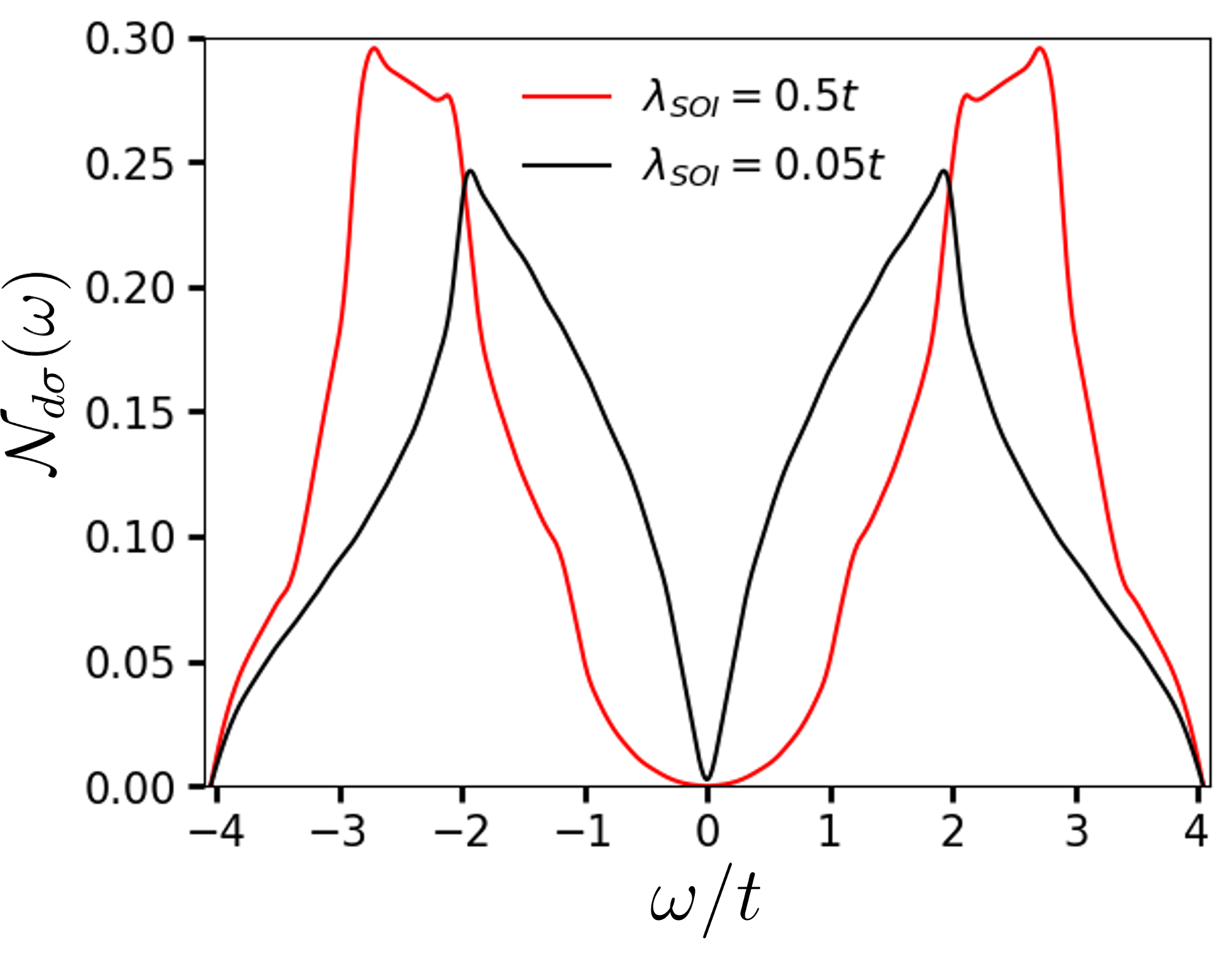
In Fig. 13, the density of states of the non-interacting system is shown for increasing . Using (92) we can obtain the dependence on . One finds that decreases with due to enhancement of at high energies with increasing as observed in Fig. 13. Concomitantly (and ) increases with for similar reasons. The net effect is a suppression of with since the enhancement in occurs close to . More precisely, we find in very good agreement with the phase diagram of Fig. 2, for which . Our analysis highlights the reliability of Eq. 92 for estimating even in multiband systems.
From this analysis, we can generally conclude that if is nearly independent of as in Fig. 13, the shape of determines the behavior of . Systems where exhibits higher density of states toward higher energies close to the band edges would yield lower values of . A qualitatively similar relationship between and was found previously in the context of pyrochlore iridatesPesin and Balents (2010).
Appendix H Electron Green’s function zeros and spectral density
In this appendix, we show the explicit derivation of the non-local electron Green’s function, , for the nodal-line semimetal under the influence of electronic interactions.
In (58) we show the expression of the electron Green’s function as the convolution of the spinon and rotor Green’s functions.Wagner et al. (2024) The non-local Green’s function for the spinons and rotors, respectively, read:
| (93) | |||
| (94) |
where, for and just considering n.n. hoping:
| (95) |
being . The eigenvalues of the spinon and rotor Hamiltonians are and . Thus, considering this in (58) and performing the Matsubara sums using (87), one can get the electron Green’s function matrix:
| (96) |
in which the matrix elements in the insulating phase () read:
| (97) |
| (98) |
where: and .
Since in the metallic phase, the coherent part of the Green’s function, plays a role, and reads:
Thus, performing the analytical continuation , one is able to compute the determinant of the non-local electron Green’s function shown in Fig. 10. The spectral density function, , which instead involves the local Green’s function, ,Fernández López and Merino (2022); López et al. (2024) is also shown.
References
- Raghu et al. (2008) S. Raghu, X.-L. Qi, C. Honerkamp, and S.-C. Zhang, Topological Mott Insulators, Phys. Rev. Lett. 100, 156401 (2008).
- Chen et al. (2021a) B.-B. Chen, Y. D. Liao, Z. Chen, O. Vafek, J. Kang, W. Li, and Z. Y. Meng, Topological Mott Insulators, Nat. Comm. 12, 5480 (2021a).
- Pesin and Balents (2010) D. Pesin and L. Balents, Mott physics and band topology in materials with strong spin–orbit interaction, Nature Physics 6, 376–381 (2010).
- Fu et al. (2007a) L. Fu, C. L. Kane, and E. J. Mele, Topological Insulators in Three Dimensions, Phys. Rev. Lett. 98, 106803 (2007a).
- Young et al. (2012) S. M. Young, S. Zaheer, J. C. Y. Teo, C. L. Kane, E. J. Mele, and A. M. Rappe, Dirac Semimetal in Three Dimensions, Phys. Rev. Lett. 108, 140405 (2012).
- Zhang et al. (2009) Y. Zhang, Y. Ran, and A. Vishwanath, Topological insulators in three dimensions from spontaneous symmetry breaking, Phys. Rev. B 79, 245331 (2009).
- Kargarian and Fiete (2013) M. Kargarian and G. A. Fiete, Topological Crystalline Insulators in Transition Metal Oxides, Phys. Rev. Lett. 110, 156403 (2013).
- Maciejko and Fiete (2015) J. Maciejko and G. A. Fiete, Fractionalized topological insulators, Nature Physics 11, 385 (2015).
- Bergman et al. (2007) D. Bergman, J. Alicea, E. Gull, S. Trebst, and L. Balents, Order-by-disorder and spiral spin-liquid in frustrated diamond-lattice antiferromagnets, Nat. Phys. 3, 487 (2007).
- Shimizu et al. (2019) Y. Shimizu, A. Otsuka, M. Maesato, M. Tsuchiizu, A. Nakao, H. Yamochi, T. Hiramatsu, Y. Yoshida, and G. Saito, Molecular diamond lattice antiferromagnet as a Dirac semimetal candidate, Phys. Rev. B 99, 174417 (2019).
- Wagner et al. (2023) N. Wagner, L. Crippa, A. Amaricci, P. Hansmann, M. Klett, E. J. König, T. Schäfer, D. D. Sante, J. Cano, A. J. Millis, A. Georges, and G. Sangiovanni, Topological Green’s Function Zeros in an Exactly Solved Model and Beyond, Nat. Comm. 14, 7531 (2023).
- Wagner et al. (2024) N. Wagner, D. Guerci, A. J. Millis, and G. Sangiovanni, Edge Zeros and Boundary Spinons in Topological Mott Insulators, Phys. Rev. Lett. 133, 126504 (2024).
- Kiswandhi et al. (2020a) A. Kiswandhi, M. Maesato, S. Tomeno, Y. Yoshida, Y. Shimizu, P. Shahi, J. Gouchi, Y. Uwatoko, G. Saito, and H. Kitagawa, High pressure investigation of an organic three-dimensional Dirac semimetal candidate having a diamond lattice, Phys. Rev. B 101, 245124 (2020a).
- Otsuka et al. (2020) A. Otsuka, Y. Shimizu, G. Saito, M. Maesato, A. Kiswandhi, T. Hiramatsu, Y. Yoshida, H. Yamochi, M. Tsuchiizu, Y. Nakamura, H. Kishida, and H. Ito, Canting Antiferromagnetic Spin-Order ( K) in a Monomer Mott Insulator (ET)Ag4(CN)5 with a Diamond Spin-Lattice, Bulletin of the Chemical Society of Japan 93, 260 (2020).
- Vanderbilt (2018) D. Vanderbilt, Berry Phases in Electronic Structure Theory: Electric Polarization, Orbital Magnetization and Topological Insulators (Cambridge University Press, 2018).
- Bzdušek and Sigrist (2017) T. Bzdušek and M. Sigrist, Robust doubly charged nodal lines and nodal surfaces in centrosymmetric systems, Phys. Rev. B 96, 155105 (2017).
- Fang et al. (2015) C. Fang, Y. Chen, H.-Y. Kee, and L. Fu, Topological nodal line semimetals with and without spin-orbital coupling, Phys. Rev. B 92, 081201 (2015).
- Rui et al. (2018a) W. B. Rui, Y. X. Zhao, and A. P. Schnyder, Topological transport in Dirac nodal-line semimetals, Phys. Rev. B 97, 161113 (2018a).
- García (2020) M. A. García, Topological Phases and Magnetic Order in Orthorhombic Diamond Lattices, Master’s thesis, Universidad Autónoma de Madrid (2020).
- Chan et al. (2016) Y.-H. Chan, C.-K. Chiu, M. Y. Chou, and A. P. Schnyder, and other topological semimetals with line nodes and drumhead surface states, Phys. Rev. B 93, 205132 (2016).
- Burkov et al. (2011) A. A. Burkov, M. D. Hook, and L. Balents, Topological nodal semimetals, Phys. Rev. B 84, 235126 (2011).
- Kopnin et al. (2011) N. B. Kopnin, T. T. Heikkilä, and G. E. Volovik, High-temperature surface superconductivity in topological flat-band systems, Phys. Rev. B 83, 220503 (2011).
- Chen et al. (2021b) W. Chen, L. Liu, W. Yang, D. Chen, Z. Liu, Y. Huang, T. Zhang, H. Zhang, Z. Liu, and D. W. Shen, Evidence of topological nodal lines and surface states in the centrosymmetric superconductor , Phys. Rev. B 103, 035133 (2021b).
- Muechler et al. (2020) L. Muechler, A. Topp, R. Queiroz, M. Krivenkov, A. Varykhalov, J. Cano, C. R. Ast, and L. M. Schoop, Modular Arithmetic with Nodal Lines: Drumhead Surface States in ZrSiTe, Phys. Rev. X 10, 011026 (2020).
- Hosen et al. (2020) M. M. Hosen, G. Dhakal, B. Wang, N. Poudel, K. Dimitri, F. Kabir, C. Sims, S. Regmi, K. Gofryk, D. Kaczorowski, A. Bansil, and M. Neupane, Experimental observation of drumhead surface states in SrAs3, Scientific Reports 10, 2776 (2020).
- Goikoetxea et al. (2020) J. Goikoetxea, J. Bravo-Abad, and J. Merino, Generating Weyl nodes in non-centrosymmetric cubic crystal structures, Journal of Physics Communications 4, 065006 (2020).
- Nielsen and Ninomiya (1983) H. B. Nielsen and M. Ninomiya, The Adler-Bell-Jackiw anomaly and Weyl fermions in a crystal, Physics Letters B 130, 389 (1983).
- Fu et al. (2007b) L. Fu, C. L. Kane, and E. J. Mele, Topological Insulators in Three Dimensions, Phys. Rev. Lett. 98, 106803 (2007b).
- Fu and Kane (2007) L. Fu and C. L. Kane, Topological insulators with inversion symmetry, Phys. Rev. B 76, 045302 (2007).
- Rachel and Le Hur (2010) S. Rachel and K. Le Hur, Topological insulators and Mott physics from the Hubbard interaction, Phys. Rev. B 82, 075106 (2010).
- Luttinger and Tisza (1946) J. M. Luttinger and L. Tisza, Theory of Dipole Interaction in Crystals, Phys. Rev. 70, 954 (1946).
- Luttinger (1951) J. M. Luttinger, A Note on the Ground State in Antiferromagnetics, Phys. Rev. 81, 1015 (1951).
- Litvin (1974) D. Litvin, The Luttinger-Tisza method, Physica 77, 205 (1974).
- Florens and Georges (2002) S. Florens and A. Georges, Quantum impurity solvers using a slave rotor representation, Phys. Rev. B 66, 165111 (2002).
- Fernández López and Merino (2022) M. Fernández López and J. Merino, Bad topological semimetals in layered honeycomb compounds, Phys. Rev. B 105, 115138 (2022).
- López et al. (2024) M. F. López, I. n. García-Elcano, J. Bravo-Abad, and J. Merino, Emergence of spinon Fermi arcs in the Weyl-Mott metal-insulator transition, Phys. Rev. B 109, 085137 (2024).
- Florens and Georges (2004) S. Florens and A. Georges, Slave-rotor mean-field theories of strongly correlated systems and the Mott transition in finite dimensions, Phys. Rev. B 70, 035114 (2004).
- López (2024) M. F. López, Fractionalized Topological Phases in Strongly Correlated Materials with Spin-Orbit Coupling, Phd thesis, Universidad Autónoma de Madrid, Madrid, Spain (2024), forthcoming. Available soon at https://repositorio.uam.es/.
- Liebsch (2011) A. Liebsch, Correlated Dirac fermions on the honeycomb lattice studied within cluster dynamical mean field theory, Phys. Rev. B 83, 035113 (2011).
- Wu et al. (2010) W. Wu, Y.-H. Chen, H.-S. Tao, N.-H. Tong, and W.-M. Liu, Interacting Dirac fermions on honeycomb lattice, Phys. Rev. B 82, 245102 (2010).
- Wang et al. (2017) R. Wang, A. Go, and A. J. Millis, Electron interactions, spin-orbit coupling, and intersite correlations in pyrochlore iridates, Phys. Rev. B 95, 045133 (2017).
- Song et al. (2023) Z. Song, U. F. P. Seifert, Z.-X. Luo, and L. Balents, Mott insulators in moiré transition metal dichalcogenides at fractional fillings: Slave-rotor mean-field theory, Phys. Rev. B 108, 155109 (2023).
- Ko and Lee (2011) W.-H. Ko and P. A. Lee, Magnetism and Mott transition: A slave-rotor study, Phys. Rev. B 83, 134515 (2011).
- Yang and Liu (2024) J. Yang and X.-J. Liu, Chiral spin liquid phase in an optical lattice at mean-field level, Phys. Rev. B 109, 165108 (2024).
- Bollmann et al. (2024) S. Bollmann, C. Setty, U. F. P. Seifert, and E. J. König, Topological Green’s Function Zeros in an Exactly Solved Model and Beyond, Phys. Rev. Lett. 133, 136504 (2024).
- He and Lee (2022) W.-Y. He and P. A. Lee, Magnetic impurity as a local probe of the (1) quantum spin liquid with spinon Fermi surface, Phys. Rev. B 105, 195156 (2022).
- He and Lee (2023) W.-Y. He and P. A. Lee, Electronic density of states of a quantum spin liquid with spinon Fermi surface. II. Zeeman magnetic field effects, Phys. Rev. B 107, 195156 (2023).
- Blason and Fabrizio (2023) A. Blason and M. Fabrizio, Unified role of Green’s function poles and zeros in correlated topological insulators, Phys. Rev. B 108, 125115 (2023).
- Müller et al. (2020) C. S. A. Müller, T. Khouri, M. R. van Delft, S. Pezzini, Y.-T. Hsu, J. Ayres, M. Breitkreiz, L. M. Schoop, A. Carrington, N. E. Hussey, and S. Wiedmann, Determination of the Fermi surface and field-induced quasiparticle tunneling around the Dirac nodal loop in ZrSiS, Phys. Rev. Res. 2, 023217 (2020).
- Rui et al. (2018b) W. B. Rui, Y. X. Zhao, and A. P. Schnyder, Topological transport in Dirac nodal-line semimetals, Phys. Rev. B 97, 161113 (2018b).
- Kiswandhi et al. (2020b) A. Kiswandhi, M. Maesato, S. Tomeno, Y. Yoshida, Y. Shimizu, P. Shahi, J. Gouchi, Y. Uwatoko, G. Saito, and H. Kitagawa, High pressure investigation of an organic three-dimensional Dirac semimetal candidate having a diamond lattice, Phys. Rev. B 101, 245124 (2020b).
- Yang et al. (2018) H. Yang, R. Moessner, and L.-K. Lim, Quantum oscillations in nodal line systems, Phys. Rev. B 97, 165118 (2018).