Cross-Modal Few-Shot Learning with Second-Order Neural Ordinary Differential Equations

Abstract

We introduce SONO, a novel method leveraging Second-Order Neural Ordinary Differential Equations (Second-Order NODEs) to enhance cross-modal few-shot learning. By employing a simple yet effective architecture consisting of a Second-Order NODEs model paired with a cross-modal classifier, SONO addresses the significant challenge of overfitting, which is common in few-shot scenarios due to limited training examples. Our second-order approach can approximate a broader class of functions, enhancing the model’s expressive power and feature generalization capabilities. We initialize our cross-modal classifier with text embeddings derived from class-relevant prompts, streamlining training efficiency by avoiding the need for frequent text encoder processing. Additionally, we utilize text-based image augmentation, exploiting CLIP’s robust image-text correlation to enrich training data significantly. Extensive experiments across multiple datasets demonstrate that SONO outperforms existing state-of-the-art methods in few-shot learning performance.

Introduction

Contrastive vision-language pre-training has revolutionized multimodal machine learning, establishing a new framework for integrating visual and textual data (Li et al. 2022a; Jia et al. 2021). This approach has rapidly gained traction, influencing a wide range of visual tasks such as semantic segmentation, object detection, image captioning, and classification (Yuan et al. 2021; Rao et al. 2022; Wang et al. 2022, 2023). CLIP (Radford et al. 2021), one of the most recognized vision-language models, has garnered widespread attention for its simplicity and effectiveness. Trained on large-scale image-text pairs, CLIP creates a unified embedding space by aligning visual and textual modalities, enabling strong zero-shot performance across various downstream tasks (Zhang et al. 2022; Zhu et al. 2023). However, despite its competitive performance, CLIP’s pre-trained nature limits its adaptability to unseen domains. To enhance CLIP’s performance in few-shot settings, several works have focused on fine-tuning by adding learnable modules on top of the frozen CLIP model to better handle new semantic domains.

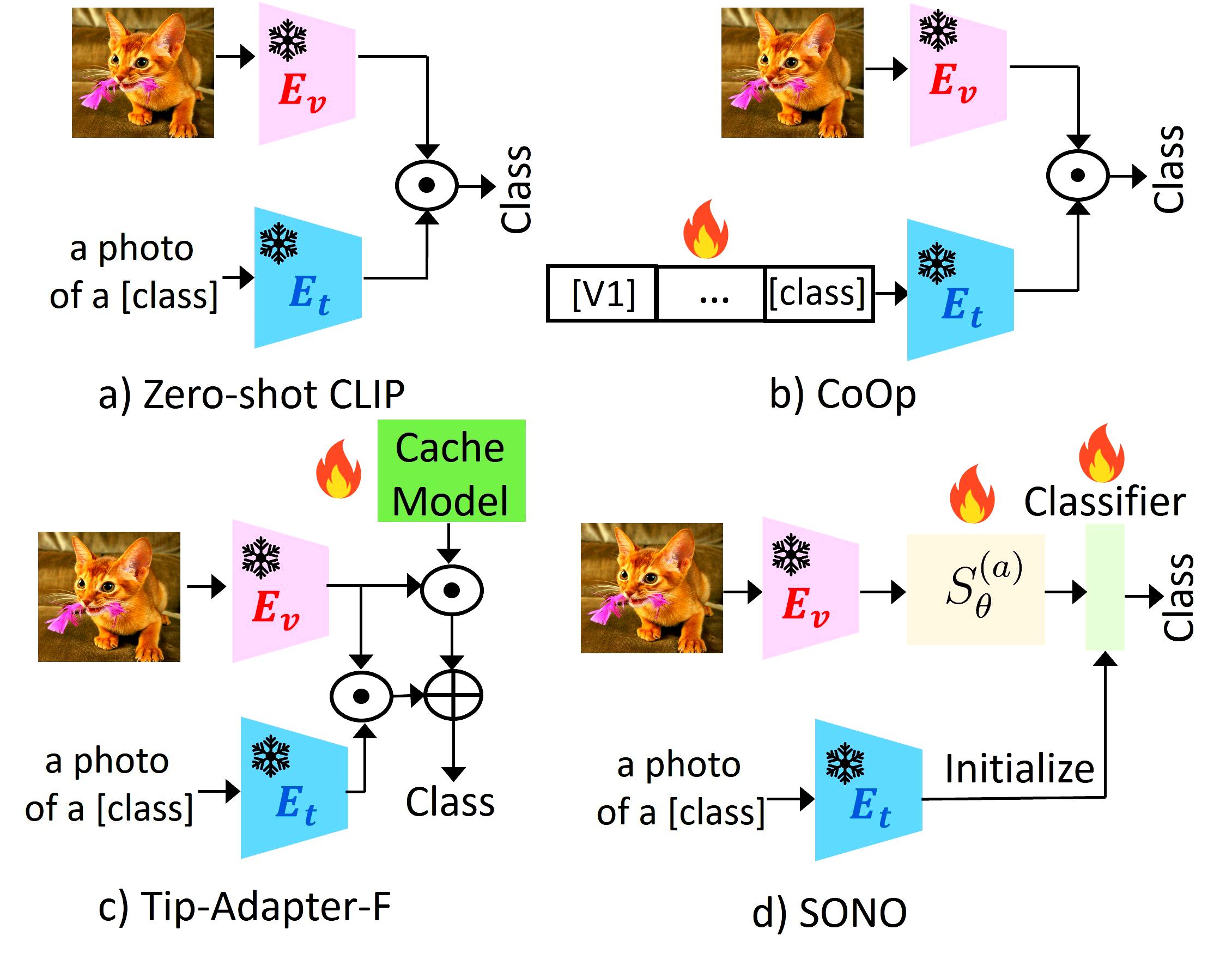
Figure 1: Comparison between (a) Zero-shot CLIP (Radford et al. 2021), (b) CoOp (Zhou et al. 2022b), (c) Tip-Adapter-F (Zhang et al. 2022), and (d) our proposed SONO, where $S^{(a)}_{\theta}$ represents the Second-Order NODE model.

Existing CLIP fine-tuning methods can be broadly categorized into two groups: 1) input-level prompting methods, such as CoOp (Zhou et al. 2022b), CoCoOp (Zhou et al. 2022a), and PLOT (Chen et al. 2023), and 2) feature-level adapting methods, like CLIP-Adapter (Gao et al. 2024), Tip-Adapter-F (Zhang et al. 2022), and GraphAdapter (Li et al. 2024). Input-level prompting methods use learnable prompts before CLIP’s text encoder to distill task-specific knowledge, while feature-level adapting methods apply residual-style adapters after CLIP’s encoders, as shown in Figure 1. However, prompting methods such as CoOp show limited few-shot accuracy and require additional training time and computational resources, while adapter-based methods like Tip-Adapter-F can be inefficient due to the large caches and extensive parameter tuning. This leads us to ask: Is it possible to achieve strong few-shot performance by adding only efficient learnable modules, making fine-tuning both effective and efficient?

To address these challenges, we propose a novel method called SONO, which is simple yet efficient. SONO introduces Second-Order Neural Ordinary Differential Equations (Second-Order NODEs) as a powerful approach for cross-modal few-shot learning, with a particular emphasis on feature optimization. Few-shot classification challenges models with very limited examples per class, leading to a high risk of overfitting in traditional neural networks. Neural Ordinary Differential Equations (NODEs) address this by modeling data transformations continuously, rather than through discrete layers. This continuous modeling enables smoother, more generalized feature transformations that are less likely to overfit. NODEs typically use fewer parameters, reducing the risk of memorizing data and further preventing overfitting. Additionally, NODEs utilize ODE solvers for dynamic time step adjustment during training, enhancing the precision of feature optimization and overall model performance.

Despite the strengths of NODEs, few-shot classification requires models with high expressive power. NODEs, limited by their inability to approximate a broad class of functions, can struggle in these tasks. This is because their ODE flows do not intersect, restricting their capability to capture complex patterns. Augmenting these to Second-Order NODEs, which are universal approximators (Kidger 2022), resolves this issue by broadening the range of functions they can model and enhancing their representational capacity. This allows for faster training and convergence. With these improvements, Second-Order NODEs maintain continuous transformation and offer a robust solution for few-shot classification, promising improved performance.

Contributions. Our contributions could be summarized as follows: 1) We introduce a novel method called SONO, which employs a simple architecture consisting of a Second-Order Neural ODE model and a cross-modal classifier. 2) We use the Second-Order NODEs for feature optimization. The cross-modal classifier is initialized with text embeddings derived from prompts containing class names. This initialization approach makes the classifier functions similarly to prompt tuning in CoOp, but it eliminates the need to process data through the text encoder in every training iteration, making our method more efficient. 3) Additionally, we adopt a strategy of using text as images for data augmentation. Given CLIP’s powerful image-text correlation capabilities and the ease of obtaining text descriptions for each class, this strategy proves to be highly effective. For each class, we select several prompts with the highest cosine similarities to the available labeled training images, using them as data augmentation for the training samples. 4) Our extensive experiments demonstrate that our proposed SONO significantly improves few-shot classification and domain generalization performance, surpassing state-of-the-art methods by a substantial margin.

Related Work

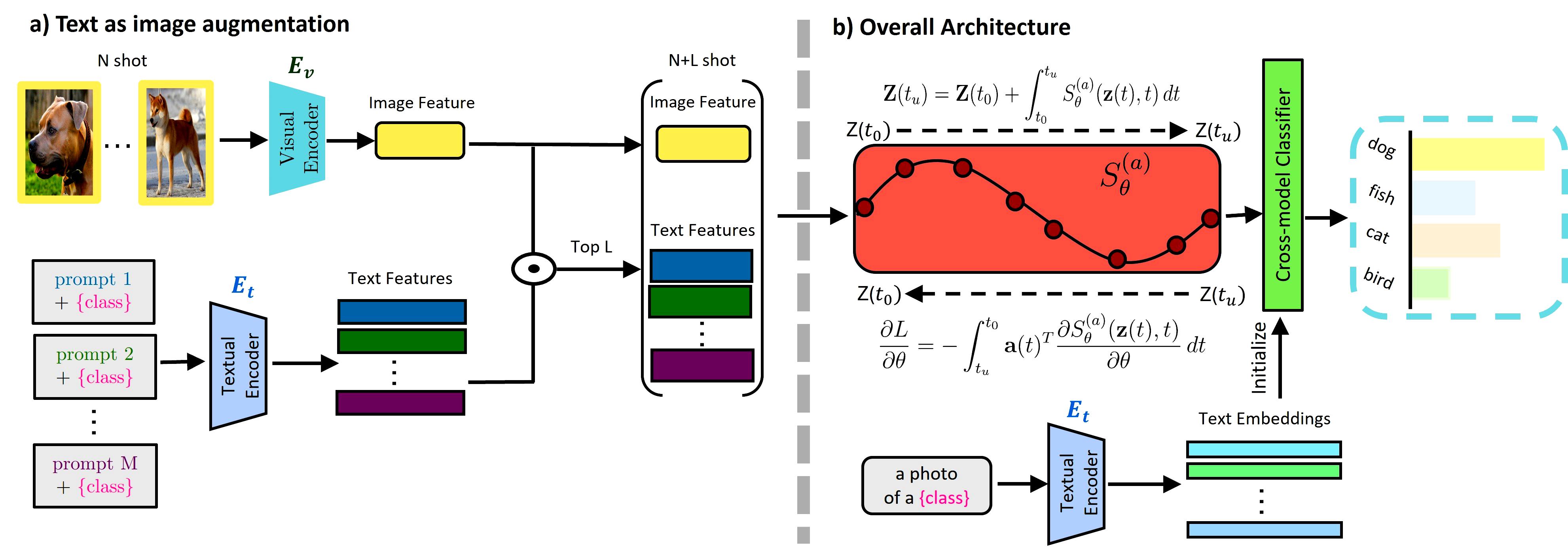
Figure 2: An overview of our method for $K$-class $N$-shot classification. Subfigure (a) illustrates the text-as-image data augmentation process. Subfigure (b) presents the overall architecture of our proposed SONO, consisting of a Second-Order NODEs model $S^{(a)}_{\theta}$ and a cross-modal classifier, which is initialized with text embeddings derived from prompts containing class labels.

Vision-Language Models (VLMs). VLMs have become a central focus in multimodal research due to their capacity to integrate visual and textual data into a shared representation space (Yang et al. 2022; Su et al. 2019; Desai and Johnson 2021). These models can be broadly classified based on their pre-training objectives into contrastive learning (Radford et al. 2021; Jia et al. 2021), generative modeling (Yu et al. 2022; Singh et al. 2022), and alignment objectives (Li et al. 2022b; Yao et al. 2022). Contrastive learning, exemplified by models such as CLIP (Radford et al. 2021) and ALIGN (Jia et al. 2021), leverages extensive image-text datasets to align visual and textual embeddings, resulting in impressive performance on zero-shot learning and other open-world tasks. In this work, we utilize CLIP (Radford et al. 2021) as the foundation for our approach.

Fine-tuning for VLMs. Recent efforts to adapt pre-trained VLMs to downstream tasks focus on two main strategies: Prompt Tuning and Feature Adaptation (Zhang et al. 2024a). Prompt tuning optimizes the input prompts, either textual or visual, to better align with downstream tasks while keeping most VLM parameters fixed. Notable examples include CoOp (Zhou et al. 2022b), which optimizes context words for each class, and CoCoOp (Zhou et al. 2022a), which conditions prompts on individual images to improve generalization. Other approaches, such as TPT (Shu et al. 2022), adapt prompts dynamically during test-time to better handle distribution shifts. Feature adaptation involves introducing lightweight adapters to refine the representations learned by VLMs. For instance, CLIP-Adapter (Gao et al. 2024) adds simple linear layers, and Tip-Adapter (Zhang et al. 2022) offers a training-free approach by directly using few-shot embeddings as a cache model, enabling efficient adaptation. Additionally, TaskRes (Yu et al. 2023) adapts the text-based classifier to better exploit the existing knowledge in the pre-trained VLM, while GraphAdapter (Li et al. 2024) leverages task-specific structures and relationships within the data for more specialized adaptation. Besides these two major approaches, methods like CuPL (Pratt et al. 2023), which uses large language models to generate more effective prompts, and CALIP (Guo et al. 2022), which introduces parameter-free attention mechanisms, offer additional innovations. This work diverges from both prompt tuning and feature adaptation, presenting a unique approach using NODEs for efficient cross-modal few-shot learning.

Neural ODEs. Neural Ordinary Differential Equations (NODEs) (Chen et al. 2018) extend the concept of Residual Networks (ResNets) (He et al. 2016) by considering the limit where the discretization step approaches zero. This approach naturally leads to the formulation of an Ordinary Differential Equations (ODEs), which can be optimized using black-box ODE solvers. The continuous-depth nature of NODEs makes them exceptionally well-suited for learning and modeling the unknown dynamics of complex systems, which are often difficult to describe analytically. It has been applied to Vision-Language Reasoning (Zhang et al. 2024b). However, numerous dynamical systems encountered in scientific research, including Newton’s equations of motion and various oscillatory systems, are primarily governed by Second-Order ODEs. (Massaroli et al. 2020) demonstrated that higher-order systems exhibit greater parameter efficiency. Furthermore, (Norcliffe et al. 2020) conducted a comprehensive study on Second-Order behaviors, concluding that these systems perform better. Applications of these models have been explored in fields such as medical segmentation (Cheng et al. 2023) and the acceleration of diffusion models (Ordoñez et al. 2024). Despite these promising outcomes, there is a conspicuous gap in the research concerning the application of VLMs. In this study, we focus on leveraging Second-Order NODEs to fine-tune VLMs and enhance feature optimization.

Method

Background

CLIP. The CLIP model (Radford et al. 2021) excels in visual tasks by mapping image and text into a joint embedding space using contrastive learning on large-scale image-text pairs. CLIP’s encoders, $\{E_{t},E_{v}\}$, include a text encoder $E_{t}$ (usually a Transformer (Vaswani et al. 2017)) and an image encoder $E_{v}$ (typically a ResNet (He et al. 2016) or ViT (Dosovitskiy et al. 2020)). In a zero-shot classification setting with $N$ classes, given a test image $x_{test}$, the visual feature $f_{v}=E_{v}(x_{test})$ is extracted, and $N$ text features $f_{t_{i}}=E_{t}(\{\pi;y_{i}\})$ are generated, where $y_{i}$ is appended to a prompt $\pi$, (e.g.,“a photo of a”). The probability of $x_{test}$ belonging to $y_{i}$ is calculated as:

$$p(y=y_{i}|x_{test})=\frac{\exp\left(\mathrm{sim}\left(f_{t_{i}},f_{v}\right)/\tau\right)}{\sum\nolimits_{t^{\prime}}{\exp\left(\mathrm{sim}\left(f_{t^{\prime}},f_{v}\right)/\tau\right)}},$$ (1)

where $\tau$ is the softmax temperature and $\mathrm{sim}(\cdot,\cdot)$ denotes cosine similarity.

Cross-modal Few-shot Learning with Second-Order Neural Ordinary Differential Equations (SONO)

Method Overview. In Figure 2, we provide an overview of our proposed SONO. Figure 2(a) illustrates the Text-as-Image Augmentation process. Leveraging CLIP’s strong image-text correlation capabilities, we use text for data augmentation. For a $K$-class $N$-shot few-shot learning problem, given a class $k$ and a list of prompts containing class labels $\Psi$ collected from CLIP (Radford et al. 2021) and CuPL (Pratt et al. 2023), we select $L$ prompts from the $M$ available for each class using cosine similarity as the augmentation for class $k$. The overall architecture of SONO is shown in Figure 2(b). SONO consists of a Second-Order Neural ODE model for feature optimization and a cross-modal classifier for classification. Given a feature sample from the augmented training features from (a), it is first input into the Second-Order Neural ODE model to refine the feature, then the refined feature is fed into the cross-modal classifier for the final prediction. The classifier is initialized with text embeddings derived from prompts containing class labels.

Second-Order Neural ODEs for Better Features

This section details the mathematical foundation of Second-Order Neural ODEs for Better Features, providing a detailed exploration of the underlying principles that enable these models to effectively refine features.

In our framework, we define our model as follows:

$$\left\{\begin{array}[]{l}\mathbf{x}^{\prime\prime}(t)=S_{\theta}^{(a)}\left(\mathbf{x}(t),\mathbf{x}^{\prime}(t),t\right)\\ \mathbf{x}(t_{0})=x_{0},~~~\mathbf{x}^{\prime}(t_{0})=g_{\theta}(x(t_{0})),\end{array}\right.$$ (2)

where $S_{\theta}^{(a)}$ is typically a neural network parameterized by $\theta$, $\mathbf{x}(t_{0})$ and $\mathbf{x}^{\prime}(t_{0})$ are the two initial conditions. We first explore the computational aspects of (2). This model employs ODE solvers in both forward pass and backpropagation. However, ODE solvers only allow the use of first-order ordinary differential equations. Therefore, we need to transform our model into a system of first order NODEs first. To represent (2) as a system of first-order NODEs, we introduce the state vector $\mathbf{z}(t)$: $\mathbf{z}(t)=[\mathbf{x}(t),\mathbf{x}^{\prime}(t)]^{T}$ $\implies$ $\mathbf{z}^{\prime}(t)=[x^{\prime}(t),S_{\theta}^{(a)}\left(\mathbf{x}(t),\mathbf{x}^{\prime}(t),t\right)]^{T}=S_{\theta}^{(v)}(\mathbf{z},t,\theta_{f})$ with the initial condition: $\mathbf{z}(t_{0})=[X_{0},g(X_{0},\theta_{g})]^{T}$. We can now apply the ODE solvers. Given an initial feature $\mathbf{z}(t_{0})$, our objective is to refine this feature progressively until we obtain the final optimal feature, denoted as $\mathbf{z}(t_{u})$. The feature $\mathbf{z}(t_{0})$ was derived from the Text-as-Image Augmentation process, whereas the feature $\mathbf{z}(t_{u})$ was subsequently updated by the ODE solver at the final time step. In the context of the ODE solver, the fourth-order Runge-Kutta method (RK4) method was selected due to its well-known convergence rate and enhanced stability properties. Additionally, the maximum time step for the ODE solvers was set to 1000, indicating that the maximum value of $u$ is 1000. The ODE solver was employed in both the forward pass and backpropagation processes.

Forward Pass. In the forward pass, the problem is reduced to solving an ordinary differential equation (ODE) initial value problem. This is addressed by integrating the ODE from the initial time $t_{0}$ to the final time $t_{u}$, using an ODE solver as governed by the following equation: $\mathbf{Z}(t_{u})=\mathbf{Z}(t_{0})+\int_{t_{0}}^{t_{u}}S_{\theta}^{(a)}(\mathbf{z}(t),t)\,dt$. This expression implies that: $\mathbf{Z}(t_{u})=\text{ODESolve}(\mathbf{z}(t_{0}),S_{\theta}^{(a)},t_{0},t_{u})$, where the function $\text{ODESolve}(\cdot)$ denotes the ODE solver.

Backpropagation. The loss function can also be formulated as an integration problem, which can subsequently be solved using another ODE solver. This process involves reversing the time steps, starting from $t_{u}$ and proceeding to $t_{0}$. The loss value can be determined using the following expression: $L(\textbf{z}(t_{u}))=L\left(\textbf{z}(t_{0})+\int_{t_{0}}^{t_{u}}S_{\theta}^{(a)}(\textbf{z}(t),t)\,dt\right)$, which can be equivalently represented as: $L(\textbf{z}(t_{u}))=L\left(\text{ODESolve}(\textbf{z}(t_{0}),S_{\theta}^{(a)},t_{0},t_{u})\right)$. The gradient is computed using the adjoint sensitivity method, which offers benefits such as constant memory cost and reduced numerical error. In particular, we employ the first-order adjoint method, as it has been shown to be more efficient, requiring fewer matrix computations compared to the Second-Order adjoint method, as demonstrated by (Norcliffe et al. 2020). We have previously transformed (2) into a system of first-order ordinary differential equations (ODEs), thereby enabling the direct application of the first-order adjoint method. We can compute the gradient by $\frac{\partial L}{\partial\theta}=-\int_{t_{u}}^{t_{0}}\mathbf{a}(t)^{T}\frac{\partial S_{\theta}^{(a)}(\mathbf{z}(t),t)}{\partial\theta}\,dt$, where $\mathbf{a}(t)=\frac{\partial L}{\partial z(t)}$ and $\frac{d\mathbf{a}(t)}{dt}=-\mathbf{a}(t)^{T}\,\frac{\partial S_{\theta}^{(a)}(\mathbf{z}(t),t)}{\partial\mathbf{z}}$. The integrals required for determining $\mathbf{z}$, $\mathbf{a}$ and $\frac{\partial L}{\partial\theta}$ can be efficiently computed in a single call of an ODE solver. This approach involves concatenating the original state, the adjoint state, and the additional partial derivatives into a unified vector, enabling simultaneous calculation.

Text-as-Image Augmentation.

CLIP establishes a robust shared image-text feature space, trained on large-scale image-text pairs, giving it powerful image-text correlation capabilities. Motivated by this unique characteristic, we propose using text as a form of data augmentation in this paper. Since text is easier and more efficient to obtain compared to images, this approach offers a practical and effective solution for augmenting data.

Specifically, we first build a prompt codebook, denoted as $\Psi\triangleq\{\psi_{k}\}_{k=1}^{K}$, where $\psi_{k}$ represents the prompt collection for class $k$. For each class, we select $M$ prompts from CLIP (Radford et al. 2021) and CuPL (Pratt et al. 2023). For example, for the class tiger shark, a prompt from CLIP might be “a photo of a tiger shark”, while a prompt form CuPL could be “A tiger shark typically has a dark blue or dark green upper body, with a light-colored underbelly”. Given $N$ shots input images belonging to class $k$, we first exploit the image encoder $E_{v}$ to extract their image features $f_{v}$, and then calculate the average of these image features. We regard the average feature as the class prototype $f_{v}^{k}$. Then, we use the text encoder $E_{t}$ to generate the textual features $\{f_{t}^{m}\}_{m=1}^{M}$ from the prompts for class $k$ in $\Psi$. We calculate the cosine similarity between the image feature $f_{v}^{k}$ and the textual features by $\mathrm{sim}\left(f_{v}^{k},f_{t}\right)=\frac{f_{t}\cdot f_{v}^{k}}{\|f_{t}\|\|f_{v}^{k}\|}$. Next, we select the textual features which have the Top-$L$ similarity with the feature of the input image, using them as the augmentation features for class $k$. For example, for the $N$-shot setting, now we have $N+L$ features for training.

Cross-Modal Few-Shot Learning

The previous section introduced the Second-Order Neural ODE model, $\mathcal{S}^{(a)}_{\theta}(x)$. After the Text-as-Image Augmentation process, we obtain $N+L$ training features, denoted as $F_{a}\triangleq\{f_{a}^{i}\}_{i=1}^{N+L}$. It is important to note that these features are L2 normalized. We next outline the training process for cross-modal few-shot learning. We begin by creating text samples by attaching the class label $y_{k}$ to a hand-crafted prompt such as $\pi=$ “a photo of a”. This process produces the text descriptions $t_{k}=\{\pi;y_{k}\}$ for each class $y_{k}$ in all $K$ classes.

During training, based on the features $F_{a}$, we learn a Second-Order Neural ODE model $\mathcal{S}^{(a)}_{\theta}(x)$ for optimizing the training features, and a cross-modal classifier $\phi$ for image classification. The classifier can be denoted as:

$$\phi(x)=W^{\top}x,$$ (3)

where $W$ represents the parameters of the cross-modal classifier $\phi$. These parameters are initialized using text features, with $w_{y_{k}}=E_{t}(t_{k}),\forall k\in[1,K]$. Here $w_{y_{k}}$ denotes the classification weight for class $y_{k}$ in the parameter matrix $W$.

Interestingly, this initialization strategy can be seen as a counterpart to prompt learning in CoOp (Zhou et al. 2022b). Since these parameters are updated during training, they function similarly to prompt learning in CoOp. By initializing with text embeddings of prompts containing class labels, this approach eliminates the need to process data through the text encoder in each training iteration, making our method more efficient and effective.

The weights in $\phi$ and $\mathcal{S}^{(a)}_{\theta}$ can be updated by gradient descent with the following cross-entropy loss during training:

$$\begin{split}\mathcal{L}_{CE}&=\sum_{i=1}^{n}{H\left(y_{k},\phi\left(\mathcal{S}^{(a)}_{\theta}\left(f_{a}^{i}\right)\right)\right)}\\ &=-\sum_{i=1}^{n}{\log\left(\frac{e^{w_{y_{k}}\cdot\mathcal{S}^{(a)}_{\theta}\left(f_{a}^{i}\right)}}{\sum\nolimits_{y^{\prime}}{e^{w_{y^{\prime}}\cdot\mathcal{S}^{(a)}_{\theta}\left(f_{a}^{i}\right)}}}\right)}.\end{split}$$ (4)

SONO Inference.

Given a test image $x_{test}$, we first utilize the image encoder $E_{v}$ to extract its image feature $f_{v}^{test}$, which is then input into the Second-Order Neural ODE Model $\mathcal{S}^{(a)}_{\theta}(x)$ to obtain the refined feature $\hat{f}_{v}^{test}$. The cross-modal classifier’s prediction can be denoted as

$$\mathcal{P}(y=y_{k}|x_{test})=w_{y_{k}}\cdot\hat{f}_{v}^{test},$$ (5)

where $1\leqslant k\leqslant K$ is the class index. The final predicted label for the test image $x_{test}$ is then given by $\hat{y}=\underset{y^{\prime}}{\mathrm{arg}\max}\,\mathcal{P}(y^{\prime}|x_{test})$

Experimental Results

Experimental Setting

Following established protocols (Zhou et al. 2022b; Zhang et al. 2022), we conducted experiments on 11 benchmark few-shot recognition datasets. These datasets cover a wide range of tasks, including generic object classification, fine-grained object classification, remote sensing recognition, texture classification, scene recognition, and action recognition: ImageNet (Recht et al. 2019), Caltech101 (Fei-Fei, Fergus, and Perona 2007), OxfordPets (Parkhi et al. 2012), StanfordCars (Krause et al. 2013), Flowers102 (Nilsback and Zisserman 2008), Food-101 (Bossard, Guillaumin, and Van Gool 2014), FGVC Aircraft (Maji et al. 2013), DTD (Cimpoi et al. 2014), SUN397 (Xiao et al. 2010), EuroSAT (Helber et al. 2019), and UCF101 (Soomro, Zamir, and Shah 2012). These datasets collectively serve as a robust benchmark for evaluating the few-shot learning capabilities of our model. Regarding domain generalization, we tested the model’s robustness to natural distribution shifts by training on a 16-shot ImageNet (Deng et al. 2009) and evaluating it on four out-of-distribution variants: ImageNet-V2 (Recht et al. 2019), ImageNet-Sketch (Wang et al. 2019), ImageNet-A (Hendrycks et al. 2021b), and ImageNet-R (Hendrycks et al. 2021a).

Baselines.

We comprehensively compare our proposed SONO with state-of-the-art methods for vision-language models, including CLIP (Radford et al. 2021), CoOp (Zhou et al. 2022b), PLOT (Chen et al. 2023), CLIP-Adapter (Gao et al. 2024), Tip-Adapter-F (Zhang et al. 2022), TaskRes (Yu et al. 2023), and GraphAdapter (Li et al. 2024). CoOp and PLOT are categorized as prompt learning methods, while TaskRes, CLIP-Adapter, Tip-Adapter-F, and GraphAdapter fall under adapter-style methods.

Implementation Details.

We utilize CLIP (Radford et al. 2021) as the base model, which consists of a ResNet-50 or ViT-B/16 image encoder and transformer text encoder. During training, we freeze the weights of CLIP to leverage its pre-trained knowledge. Following CoOp (Zhou et al. 2022b), we adopt the data preprocessing protocol from CLIP (Radford et al. 2021). we empirically set $M=50$ and $h=10$. Our experiments use standard few-shot protocols with random selections of 1, 2, 4, 8, and 16 examples per class for training, followed by evaluation on the full test set. For domain generalization, we use the model trained on 16-shot ImageNet to evaluate its performance on four variants. We train our model for 20 epochs on ImageNet and 15 epochs on the other 10 datasets, using an initial learning rate of $1\times 10^{-3}$. We optimize the model with the AdamW (Kingma and Ba 2015) optimizer and a cosine annealing scheduler. Our approach is parameter-efficient and lightweight, requiring only a single NVIDIA RTX 3090 GPU for training. Additional implementation details are provided in the Supplemental Materials.

Performance Comparison

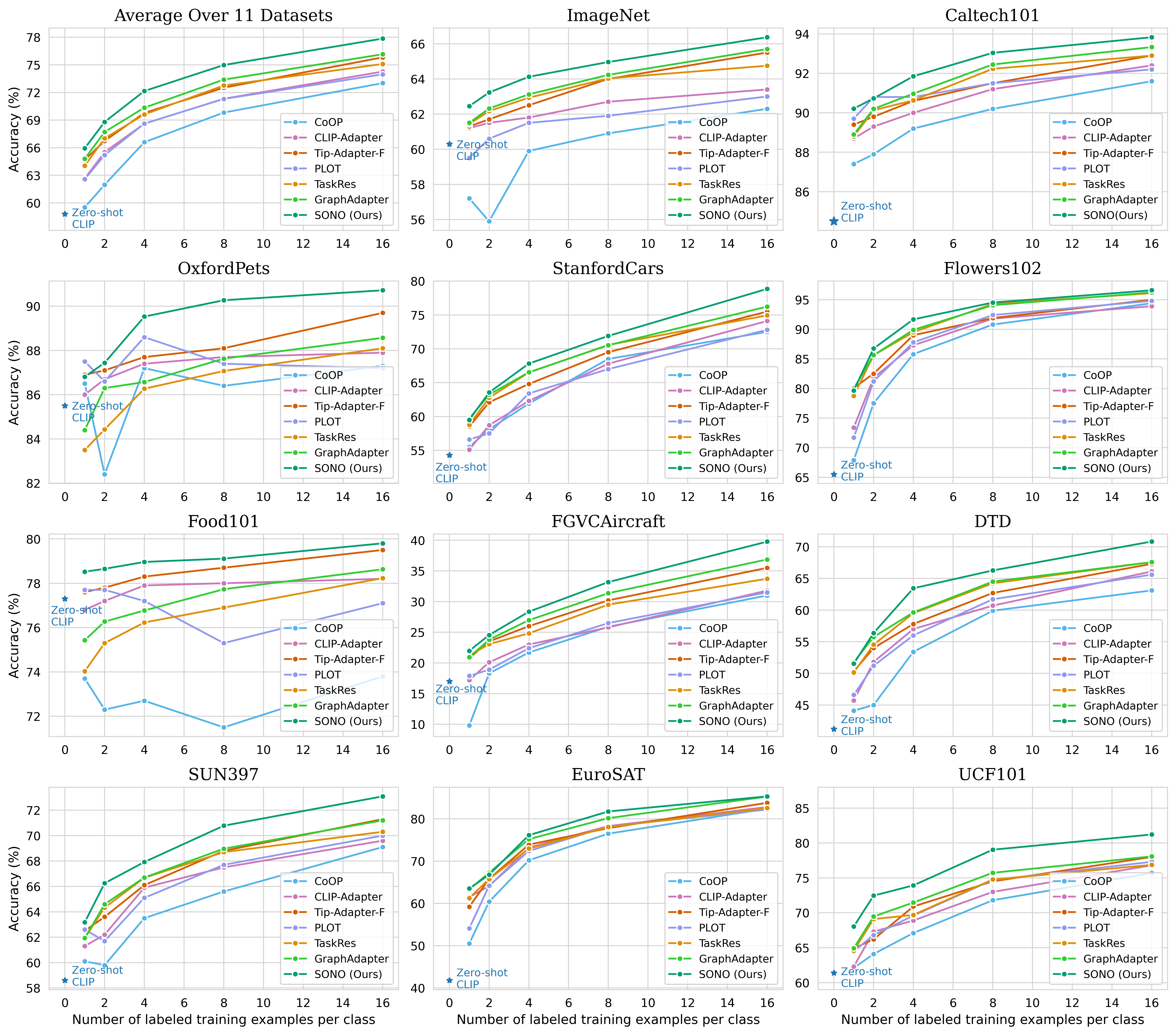
Figure 3: Classification Performance Comparison on Few-shot Learning, i.e., 1-/2-/4-/8-/16-shot, on 11 benchmark datasets. The top-left is the averaged accuracy over the 11 datasets.

Few shot Recognition.

As shown in Figure 3, we conduct a comprehensive evaluation of our proposed SONO across 11 datasets, each representing different tasks. We compare SONO with seven state-of-the-art methods, including both prompt learning and adapter-style approaches. The top-left sub-figure of Figure 3 illustrates the average accuracy results. Obviously, our proposed SONO method yields superior performance, consistently and substantially outperforming other methods from 1 to 16 shots, highlighting SONO’s strong few-shot adaptation capability. In the 16-shot setting, SONO achieves an average performance of 77.86%. This outperforms GraphAdapter (Li et al. 2024) by 1.63% and Tip-Adapter (Zhang et al. 2022) by 2.75%. Moreover, the performance gain reaches 4.7% compared to CoOp (Zhou et al. 2022b). For the largest dataset, ImageNet, SONO outperforms the second-best method, GraphAdapter, by 0.67%. On the most challenging datasets—FGVC Aircraft, DTD, and UCF101—our method achieves performance gains of up to 2.91%, 3.26%, and 3.14%, respectively. The comprehensive results demonstrate the effectiveness and robust performance of SONO.

Table 1: Performance comparisons of domain generalization on two CLIP visual backbones. All models are trained on 16-shot ImageNet and tested on cross-domain datasets, including ImageNet-V2, -Sketch, -A, and -R.

Method	Backbone	Source		Target
		ImageNet		-V2	-Sketch	-A	-R	Average
Zero-shot CLIP	ResNet-50	60.33		51.34	33.32	21.65	56.00	40.58
Linear Probe CLIP		55.87		45.97	19.07	12.74	28.16	28.16
CoOp		62.95		55.11	32.74	22.12	54.96	41.23
TaskRes		64.75		56.47	35.83	22.80	60.70	43.95
GraphAdapter		65.70		56.58	35.89	23.07	60.86	44.10
Ours		66.37		57.83	37.07	27.02	60.75	45.68
Zero-shot CLIP	ViT-B/16	67.83		60.83	46.15	47.77	73.96	57.18
Linear Probe CLIP		65.85		56.26	34.77	35.68	58.43	46.29
CoOp		71.92		64.18	46.71	48.41	74.32	58.41
TaskRes		73.07		65.30	49.13	50.37	77.70	60.63
GraphAdapter		73.68		66.60	49.23	50.75	77.73	60.78
Ours		74.92		67.33	51.15	52.96	78.88	62.58

Domain Generalization.

Table 1 presents a comparison of the performance of our method against various baseline models. We provide classification results for the source domain (ImageNet (Deng et al. 2009)) and several target domains: ImageNet-V2 (Recht et al. 2019), ImageNet-Sketch (Wang et al. 2019), ImageNet-A (Hendrycks et al. 2021b), and ImageNet-R (Hendrycks et al. 2021a). Additionally, we report the average accuracy across the out-of-distribution (OOD) datasets. Compared to the second-best method, GraphAdapter (Li et al. 2024), our method improves the OOD average accuracy by 1.58% on ResNet-50 and 1.80% on ViT-B/16. Notably, we achieve a performance gain of up to 3.95% on ImageNet-A. These results demonstrate that our SONO method exhibits exceptional robustness to distribution shifts.

Ablation Studies

We present an empirical analysis here. Unless specified, our experiments are conducted on the 16-shot ImageNet.

Contributions of Major Algorithm Components.

In Table 2, TAI stands for Text-Image Augmentation, SNM refers to the Second-Order NODEs, and the last row indicates a setup where only the classifier is retained. We conduct an ablation study by removing different components from our method to assess their impact. The first row shows the final performance of SONO during inference on the 16-shot dataset. In the first ablation, removing TAI from SONO causes a performance drop of 0.71%, emphasizing the importance of text-image augmentation. Next, we retain TAI but remove SNM, which optimizes input features for classification. This results in a 3.11% decrease in performance, highlighting the significance of the Second-Order Neural ODE model. In the last row, with both TAI and SNM removed, accuracy drops to 62.35%. Overall, these results demonstrate that each component significantly enhances performance.

Table 2: Effectiveness of different algorithm components in SONO. TAI stands for Text-Image Augmentation, and SNM refers to the Second-Order Neural ODE model. The last row represents the setup where only the classifier is retained. We conducted experiments on ImageNet and reported the accuracy.

TIA	SNM	1-shot	2-shot	4-shot	8-shot	16-shot
✓	✓	62.45	63.23	64.12	64.96	66.37
✗	✓	60.81	61.72	62.85	63.77	65.66
✓	✗	58.82	59.19	60.38	61.57	63.26
✗	✗	57.65	58.38	59.66	60.76	62.35

Evaluation on Various Visual Backbones.

Table 3 summarizes the results on the 16-shot ImageNet (Deng et al. 2009) using various visual backbones, including ResNets (He et al. 2016) and ViTs (Dosovitskiy et al. 2020). Our approach significantly improves performance, particularly when compared to zero-shot CLIP on the latest visual backbones. Additionally, our method consistently outperforms Tip-Adapter-F across all tested visual backbones.

Table 3: Evaluation of various visual backbones

Backbone	ResNet-50	ResNet-101	ViT-B/32	ViT-B/16
Zero-shot CLIP	60.33	62.53	63.80	67.83
CLIP-Adapter	63.59	65.39	66.19	71.13
Tip-Adapter-F	65.51	68.56	68.65	73.69
SONO (Ours)	66.37	69.15	69.71	74.86

Residual Ratio $\eta$.

The hyperparameter $\eta$ controls the balance between the transformed features and the original features from the visual encoder when forming the final visual features. A larger $\eta$ indicates greater reliance on the transformed features. As shown in Table 4, classification accuracy improves as $\eta$ increases from 0.0, peaking at 66.37% when $\eta=0.6$. This suggests that the transformed features generated by the Second-Order Neural ODE significantly enhance the final prediction.

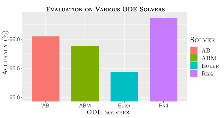
Figure 4: Ablation results on various ODE solvers: Fourth-Order Runge-Kutta (RK4), Euler, Explicit Adams-Bashforth (AB), and Implicit Adams-Bashforth-Moulton (ABM) methods.

Table 4: Sensitivity of hyperparameters. All the results are reported on a $16$-shot setting on ImageNet.

Sensitivity of Hyperparameters $\eta$ 0.0 0.2 0.4 0.6 0.8 1.0 Acc. 64.06 65.51 66.20 66.37 66.12 65.93

Table 5: Efficiency comparisons on 16-shot ImageNet. We report the results using only a NVIDIA RTX 3090 GPU.

Method	Epochs	Training	GFLOPs	Param.	Acc.	Gain
CoOp	200	15 h	$>$10	0.01M	62.95	-
CLIP-Adapter	200	50 min	0.004	0.52M	63.59	+0.64
Tip-Adapter-F	20	5 min	0.030	16.3M	65.51	+2.56
SONO(Ours)	20	3.5 min	0.010	1.54M	66.37	+3.42

Evaluation on Various ODE Solvers.

Figure 4 presents the results of different ODE solvers on the 16-shot ImageNet dataset. Our qualitative analysis aligns with the empirical findings, indicating that the RK4 outperforms the Euler, AB, and ABM methods.

Efficiency Comparison.

To demonstrate the exceptional fine-tuning efficiency of our method, we compare it against other state-of-the-art approaches, considering training epochs, training time, computational cost, and the number of parameters. The detailed results are presented in Table 5. Our SONO method reaches an accuracy of 66.37% on 16-shot ImageNet in just 3.5 minutes, using 1.54 million parameters. In comparison, CoOp needs about 15 hours of training to achieve 62.95% accuracy, while Tip-Adapter-F takes 5 minutes and requires 16.3 million parameters to achieve 65.51% accuracy. Additional details are provided in the Supplemental Materials.

Conclusion

We introduce SONO, a method for cross-modal few-shot learning, addressing the critical challenge of overfitting with limited data. By leveraging Second-Order NODEs with an efficient cross-modal classifier, SONO significantly enhances feature optimization and generalization capabilities. Utilizing text-based image augmentation further strengthens the training process, optimizing the model’s performance across diverse datasets. Our experiments demonstrate that SONO not only surpasses existing few-shot learning models but also shows proficiency in domain generalization.

References

- Bossard, Guillaumin, and Van Gool (2014) Bossard, L.; Guillaumin, M.; and Van Gool, L. 2014. Food-101–mining discriminative components with random forests. In European Conference on Computer Vision. Springer.
- Chen et al. (2023) Chen, G.; Yao, W.; Song, X.; Li, X.; Rao, Y.; and Zhang, K. 2023. Prompt Learning with Optimal Transport for Vision-Language Models. In ICLR.
- Chen et al. (2018) Chen, R. T.; Rubanova, Y.; Bettencourt, J.; and Duvenaud, D. K. 2018. Neural ordinary differential equations. Advances in neural information processing systems, 31.
- Cheng et al. (2023) Cheng, C.-W.; Runkel, C.; Liu, L.; Chan, R. H.; Schönlieb, C.-B.; and Aviles-Rivero, A. I. 2023. Continuous u-net: Faster, greater and noiseless. arXiv:2302.00626.
- Cimpoi et al. (2014) Cimpoi, M.; Maji, S.; Kokkinos, I.; Mohamed, S.; and Vedaldi, A. 2014. Describing textures in the wild. In Proceedings of the IEEE/CVF Conference on Computer Vision and Pattern Recognition.
- Deng et al. (2009) Deng, J.; Dong, W.; Socher, R.; Li, L.-J.; Li, K.; and Fei-Fei, L. 2009. Imagenet: A large-scale hierarchical image database. In 2009 IEEE conference on computer vision and pattern recognition. Ieee.
- Desai and Johnson (2021) Desai, K.; and Johnson, J. 2021. Virtex: Learning visual representations from textual annotations. In Proceedings of the IEEE/CVF Conference on Computer Vision and Pattern Recognition.
- Dosovitskiy et al. (2020) Dosovitskiy, A.; Beyer, L.; Kolesnikov, A.; Weissenborn, D.; Zhai, X.; Unterthiner, T.; Dehghani, M.; Minderer, M.; Heigold, G.; Gelly, S.; et al. 2020. An image is worth 16x16 words: transformers for image recognition at scale. In International Conference on Learning Representations.
- Fei-Fei, Fergus, and Perona (2007) Fei-Fei, L.; Fergus, R.; and Perona, P. 2007. Learning generative visual models from few training examples: An incremental Bayesian approach tested on 101 object categories. Computer Vision and Image Understanding, 106(1).
- Gao et al. (2024) Gao, P.; Geng, S.; Zhang, R.; Ma, T.; Fang, R.; Zhang, Y.; Li, H.; and Qiao, Y. 2024. Clip-adapter: Better vision-language models with feature adapters. International Journal of Computer Vision, 132.
- Guo et al. (2022) Guo, Z.; Zhang, R.; Qiu, L.; Ma, X.; Miao, X.; He, X.; and Cui, B. 2022. Calip: Zero-shot enhancement of clip with parameter-free attention. arXiv preprint arXiv:2209.14169.
- He et al. (2016) He, K.; Zhang, X.; Ren, S.; and Sun, J. 2016. Deep residual learning for image recognition. In Proceedings of the IEEE/CVF Conference on Computer Vision and Pattern Recognition.
- Helber et al. (2019) Helber, P.; Bischke, B.; Dengel, A.; and Borth, D. 2019. Eurosat: A novel dataset and deep learning benchmark for land use and land cover classification. IEEE Journal of Selected Topics in Applied Earth Observations and Remote Sensing, 12(7).
- Hendrycks et al. (2021a) Hendrycks, D.; Basart, S.; Mu, N.; Kadavath, S.; Wang, F.; Dorundo, E.; Desai, R.; Zhu, T.; Parajuli, S.; Guo, M.; et al. 2021a. The many faces of robustness: A critical analysis of out-of-distribution generalization. In Proceedings of the IEEE/CVF International Conference on Computer Vision.
- Hendrycks et al. (2021b) Hendrycks, D.; Zhao, K.; Basart, S.; Steinhardt, J.; and Song, D. 2021b. Natural adversarial examples. In Proceedings of the IEEE/CVF Conference on Computer Vision and Pattern Recognition.
- Jia et al. (2021) Jia, C.; Yang, Y.; Xia, Y.; Chen, Y.-T.; Parekh, Z.; Pham, H.; Le, Q.; Sung, Y.-H.; Li, Z.; and Duerig, T. 2021. Scaling up visual and vision-language representation learning with noisy text supervision. In International Conference on Machine Learning.
- Kidger (2022) Kidger, P. 2022. On neural differential equations. arXiv:2202.02435.
- Kingma and Ba (2015) Kingma, D. P.; and Ba, J. 2015. Adam: A method for stochastic optimization. International Conference on Learning Representations.
- Krause et al. (2013) Krause, J.; Stark, M.; Deng, J.; and Fei-Fei, L. 2013. 3D object representations for fine-grained categorization. In Proceedings of the IEEE/CVF International Conference on Computer Vision Workshops.
- Li et al. (2022a) Li, J.; Li, D.; Xiong, C.; and Hoi, S. 2022a. Blip: Bootstrapping language-image pre-training for unified vision-language understanding and generation. In International Conference on Machine Learning. PMLR.
- Li et al. (2022b) Li, L. H.; Zhang, P.; Zhang, H.; Yang, J.; Li, C.; Zhong, Y.; Wang, L.; Yuan, L.; Zhang, L.; Hwang, J.-N.; et al. 2022b. Grounded language-image pre-training. In CVPR, 10965–10975.
- Li et al. (2024) Li, X.; Lian, D.; Lu, Z.; Bai, J.; Chen, Z.; and Wang, X. 2024. Graphadapter: Tuning vision-language models with dual knowledge graph. Advances in Neural Information Processing Systems, 36.
- Maji et al. (2013) Maji, S.; Rahtu, E.; Kannala, J.; Blaschko, M.; and Vedaldi, A. 2013. Fine-grained visual classification of aircraft. arXiv preprint arXiv:1306.5151.
- Massaroli et al. (2020) Massaroli, S.; Poli, M.; Park, J.; Yamashita, A.; and Asama, H. 2020. Dissecting neural odes. Advances in Neural Information Processing Systems, 33.
- Nilsback and Zisserman (2008) Nilsback, M.-E.; and Zisserman, A. 2008. Automated flower classification over a large number of classes. In Indian Conference on Computer Vision, Graphics and Image Processing. IEEE.
- Norcliffe et al. (2020) Norcliffe, A.; Bodnar, C.; Day, B.; Simidjievski, N.; and Liò, P. 2020. On second order behaviour in augmented neural odes. Advances in neural information processing systems, 33.
- Ordoñez et al. (2024) Ordoñez, S. C.; Cheng, C.-W.; Huang, J.; Zhang, L.; Yang, G.; Schönlieb, C.-B.; and Aviles-Rivero, A. I. 2024. The Missing U for Efficient Diffusion Models. Transactions on Machine Learning Research.
- Parkhi et al. (2012) Parkhi, O. M.; Vedaldi, A.; Zisserman, A.; and Jawahar, C. 2012. Cats and dogs. In Proceedings of the IEEE/CVF Conference on Computer Vision and Pattern Recognition.
- Pratt et al. (2023) Pratt, S.; Covert, I.; Liu, R.; and Farhadi, A. 2023. What does a platypus look like? generating customized prompts for zero-shot image classification. In Proceedings of the IEEE/CVF International Conference on Computer Vision.
- Radford et al. (2021) Radford, A.; Kim, J. W.; Hallacy, C.; Ramesh, A.; Goh, G.; Agarwal, S.; Sastry, G.; Askell, A.; Mishkin, P.; Clark, J.; et al. 2021. Learning transferable visual models from natural language supervision. In International conference on machine learning, 8748–8763. PMLR.
- Rao et al. (2022) Rao, Y.; Zhao, W.; Chen, G.; Tang, Y.; Zhu, Z.; Huang, G.; Zhou, J.; and Lu, J. 2022. Denseclip: Language-guided dense prediction with context-aware prompting. In Proceedings of the IEEE/CVF Conference on Computer Vision and Pattern Recognition, 18082–18091.
- Recht et al. (2019) Recht, B.; Roelofs, R.; Schmidt, L.; and Shankar, V. 2019. Do imagenet classifiers generalize to imagenet? In International Conference on Machine Learning. PMLR.
- Shu et al. (2022) Shu, M.; Nie, W.; Huang, D.-A.; Yu, Z.; Goldstein, T.; Anandkumar, A.; and Xiao, C. 2022. Test-time prompt tuning for zero-shot generalization in vision-language models. In Advances in Neural Information Processing Systems, volume 35.
- Singh et al. (2022) Singh, A.; Hu, R.; Goswami, V.; Couairon, G.; Galuba, W.; Rohrbach, M.; and Kiela, D. 2022. Flava: A foundational language and vision alignment model. In Proceedings of the IEEE/CVF Conference on Computer Vision and Pattern Recognition.
- Soomro, Zamir, and Shah (2012) Soomro, K.; Zamir, A. R.; and Shah, M. 2012. UCF101: A dataset of 101 human actions classes from videos in the wild. arXiv preprint arXiv:1212.0402.
- Su et al. (2019) Su, W.; Zhu, X.; Cao, Y.; Li, B.; Lu, L.; Wei, F.; and Dai, J. 2019. Vl-bert: Pre-training of generic visual-linguistic representations. arXiv preprint arXiv:1908.08530.
- Vaswani et al. (2017) Vaswani, A.; Shazeer, N.; Parmar, N.; Uszkoreit, J.; Jones, L.; Gomez, A. N.; Kaiser, Ł.; and Polosukhin, I. 2017. Attention is all you need. In Advances in Neural Information Processing Systems, volume 30.
- Wang et al. (2019) Wang, H.; Ge, S.; Lipton, Z.; and Xing, E. P. 2019. Learning robust global representations by penalizing local predictive power. In Advances in Neural Information Processing Systems, volume 32.
- Wang et al. (2023) Wang, N.; Xie, J.; Luo, H.; Cheng, Q.; Wu, J.; Jia, M.; and Li, L. 2023. Efficient image captioning for edge devices. In Proceedings of the AAAI Conference on Artificial Intelligence, volume 37.
- Wang et al. (2022) Wang, Z.; Lu, Y.; Li, Q.; Tao, X.; Guo, Y.; Gong, M.; and Liu, T. 2022. Cris: Clip-driven referring image segmentation. In Proceedings of the IEEE/CVF conference on computer vision and pattern recognition.
- Xiao et al. (2010) Xiao, J.; Hays, J.; Ehinger, K. A.; Oliva, A.; and Torralba, A. 2010. Sun database: Large-scale scene recognition from abbey to zoo. In Proceedings of the IEEE/CVF Conference on Computer Vision and Pattern Recognition.
- Yang et al. (2022) Yang, J.; Duan, J.; Tran, S.; Xu, Y.; Chanda, S.; Chen, L.; Zeng, B.; Chilimbi, T.; and Huang, J. 2022. Vision-language pre-training with triple contrastive learning. In Proceedings of the IEEE/CVF Conference on Computer Vision and Pattern Recognition.
- Yao et al. (2022) Yao, L.; Han, J.; Wen, Y.; Liang, X.; Xu, D.; Zhang, W.; Li, Z.; Xu, C.; and Xu, H. 2022. Detclip: Dictionary-enriched visual-concept paralleled pre-training for open-world detection. Advances in Neural Information Processing Systems, 35.
- Yu et al. (2022) Yu, J.; Wang, Z.; Vasudevan, V.; Yeung, L.; Seyedhosseini, M.; and Wu, Y. 2022. Coca: Contrastive captioners are image-text foundation models. Transactions on Machine Learning Research.
- Yu et al. (2023) Yu, T.; Lu, Z.; Jin, X.; Chen, Z.; and Wang, X. 2023. Task residual for tuning vision-language models. In Proceedings of the IEEE/CVF Conference on Computer Vision and Pattern Recognition.
- Yuan et al. (2021) Yuan, X.; Lin, Z.; Kuen, J.; Zhang, J.; Wang, Y.; Maire, M.; Kale, A.; and Faieta, B. 2021. Multimodal contrastive training for visual representation learning. In Proceedings of the IEEE/CVF Conference on Computer Vision and Pattern Recognition.
- Zhang et al. (2024a) Zhang, J.; Huang, J.; Jin, S.; and Lu, S. 2024a. Vision-language models for vision tasks: A survey. IEEE Transactions on Pattern Analysis and Machine Intelligence.
- Zhang et al. (2022) Zhang, R.; Zhang, W.; Fang, R.; Gao, P.; Li, K.; Dai, J.; Qiao, Y.; and Li, H. 2022. Tip-adapter: Training-free adaption of clip for few-shot classification. In European Conference on Computer Vision. Springer.
- Zhang et al. (2024b) Zhang, Y.; Cheng, C.-W.; Yu, K.; He, Z.; Schönlieb, C.-B.; and Aviles-Rivero, A. I. 2024b. NODE-Adapter: Neural Ordinary Differential Equations for Better Vision-Language Reasoning. arXiv:2407.08672.
- Zhou et al. (2022a) Zhou, K.; Yang, J.; Loy, C. C.; and Liu, Z. 2022a. Conditional prompt learning for vision-language models. In Proceedings of the IEEE/CVF Conference on Computer Vision and Pattern Recognition.
- Zhou et al. (2022b) Zhou, K.; Yang, J.; Loy, C. C.; and Liu, Z. 2022b. Learning to prompt for vision-language models. International Journal of Computer Vision, 130(9).
- Zhu et al. (2023) Zhu, X.; Zhang, R.; He, B.; Zhou, A.; Wang, D.; Zhao, B.; and Gao, P. 2023. Not All Features Matter: Enhancing Few-shot CLIP with Adaptive Prior Refinement. arXiv preprint arXiv:2304.01195.