IXPE detection of highly polarized X-rays from the magnetar 1E 1841$-$045

Abstract

The Imaging X-ray Polarimetry Explorer (IXPE) observed for the first time highly polarized X-ray emission from the magnetar 1E 1841$-$045, targeted after a burst-active phase in August 2024. To date, IXPE has observed four other magnetars during quiescent periods, highlighting substantially different polarization properties. 1E 1841$-$045 exhibits a high, energy-dependent polarization degree, which increases monotonically from $\sim 15\%$ at $2$–$3\,\mathrm{keV}$ up to $\sim 55\%$ at $5.5$–$8\,\mathrm{keV}$, while the polarization angle, aligned with the celestial North, remains fairly constant. The broadband spectrum ($2$–$79\,\mathrm{keV}$) obtained by combining simultaneous IXPE and NuSTAR data is well modeled by a blackbody and two power-law components. The unabsorbed $2$–$8\,\mathrm{keV}$ flux ($\approx 2\times 10^{-11}\,\mathrm{erg\,cm}^{-2}\mathrm{\,s}^{-1}$) is about $10\%$ higher than that obtained from archival XMM-Newton and NuSTAR observations. The polarization of the soft, thermal component does not exceed $\approx 25\%$, and is difficult to reconcile with emission from a magnetized atmosphere. The intermediate power law is polarized at around $30\%$, consistent with predictions for resonant Compton scattering in the star magnetosphere; while, the hard power law exhibits a polarization degree exceeding $65\%$, pointing to a synchrotron/curvature origin.

1 Introduction

Magnetars are ultra-magnetized neutron stars whose high-energy emission is mainly powered by their own magnetic energy (Duncan & Thompson, 1992; Thompson & Duncan, 1993). The presence of magnetic fields up to three orders of magnitude stronger than those typically found in ordinary young neutron stars is at the basis of their enhanced X-ray emission and extreme variability phenomena on different timescales, ranging from short (tens of ms) bursts to months- or even years-long outbursts (see, e.g., Turolla et al., 2015; Kaspi & Beloborodov, 2017; Esposito et al., 2021, and references therein).

Such a strong magnetic field ($B\sim 10^{13}$–$10^{15}\,\mathrm{G}$) makes magnetars extremely interesting targets for polarimetric observations in the X-ray range, which have been recently made possible by the NASA-ASI Imaging X-ray Polarimetry Explorer (IXPE; Weisskopf et al., 2022). Radiation in a strongly magnetized medium propagates in the ordinary (O) and extraordinary (X) normal modes Gnedin et al. (1978). The opacity for X-mode photons is strongly suppressed, below the electron cyclotron energy, relative to that of the O-mode ones (see Harding & Lai, 2006, and references therein). The X-ray emission from magnetar sources is, then, expected to be substantially polarized (up to $\approx 80\%;$ Fernández & Davis, 2011; Taverna et al., 2014, 2020; Caiazzo et al., 2022).

The IXPE satellite observed four magnetars during the first two years of operations. Polarization was clearly measured in the $2$–$8\,\mathrm{keV}$ band for 4U 0142+61 (Taverna et al., 2022), 1RXS J170849.0–400910 (hereafter 1RXS J1708 for short; Zane et al., 2023) and 1E 2259$+$586 (Heyl et al., 2024), while an unexpectedly low flux prevented significant detection in SGR 1806$-$20 (Turolla et al., 2023). In the two brightest sources the polarization properties turned out to strongly depend on energy. In 1RXS J1708, the degree of polarization increases monotonically from $\approx 20\%$ to $\approx 80\%$ at a constant polarization angle making it the most polarized source detected by IXPE so far, while in 4U 0142+61 it is $\approx 15\%$ at $2$–$3\,\mathrm{keV}$, is consistent with zero around $4$–$5\,\mathrm{keV}$, where the polarization angle swings by $90^{\circ}$, and then reaches $\approx 35\%$ at $6$–$8\,\mathrm{keV}$.

All the IXPE observations described above were targeted on bright magnetars during periods of quiescence (see also Taverna & Turolla 2024 for a review of all the results). On the other hand, most magnetars exhibit periods of activity during which they emit frequent short bursts of hard X-rays accompanied by flux and spectral changes and/or anomalies in the timing properties (glitches, spin-down rate variations, pulse profile changes). Since these phenomena are probably associated with magnetospheric reconfigurations, it is interesting to explore the polarimetric properties during or after periods of activity.

The recent reactivation of the magnetar 1E 1841$-$045 offered this possibility. The source lies at the center of the shell-type, $4^{\prime}$-diameter supernova remnant (SNR) Kes 73, at an estimated distance of $D\approx 8.5\,\mathrm{kpc}$ Tian & Leahy (2008); Kumar & Safi-Harb (2010); Olausen & Kaspi (2014). Its X-ray luminosity $L_{\mathrm{X}}\sim 5\times 10^{35}\ \mathrm{erg}\mathrm{\,s}^{-1}$, largely in excess of the rotational energy loss rate, and the detection of pulsations suggested a magnetar interpretation (Vasisht & Gotthelf, 1997). This was confirmed by the subsequent detection of short bursts at different epochs Morii et al. (2003); Wachter et al. (2004). Very recently, after more than 9 years of inactivity (An et al., 2013; Barthelmy et al., 2015), 1E 1841$-$045 emitted a series of hard X-ray bursts, beginning on 2024 August 20th (Swift Team, 2024a, b; Fermi GBM Team, 2024; GECAM team, 2024; SVOM/GRM Team, 2024). Soft X-ray observations of the source, performed by Swift-XRT and NICER (NICER Team, 2024) about one day after the first burst, revealed an enhancement of $\sim\!25$% of the $0.5$–$10\,\mathrm{keV}$ flux with respect to the quiescent level.

In this Letter we report on an IXPE target of opportunity (ToO) observation of 1E 1841$-$045 performed soon after the burst-active phase, along with NuSTAR and archival Chandra, XMM-Newton and NuSTAR campaigns. Observations are detailed in §2 and the results of timing, spectral, and polarimetric analyses are presented in §3. Discussion follows in §4. In a companion paper (Stewart et al. 2025) an independent analysis of the same IXPE datasets is presented. The results and theoretical interpretation are largely consistent, except for the discussion on the nature of the soft X-ray component, where the two papers present distinct interpretive elements.

2 Observations and data analysis

Table 1: Log of X-ray observations and measured spin periods used in this work

Observatory	Instrument/Mode	ObsID	Start time	End time	Exposure	$P$
			(UTC)	(UTC)	(ks)	(s)
Chandra	ACIS/TE	729	2000-07-23 20:55:29	2000-07-24 05:46:55	29.26	–
Chandra	ACIS/TE	6732	2006-07-30 06:54:37	2006-07-30 14:30:26	24.86	–
Chandra	ACIS/TE	16950	2015-06-04 20:42:20	2015-06-05 05:16:21	28.69	–
Chandra	ACIS/TE	17668	2015-07-07 11:21:02	2015-07-07 17:32:53	20.89	–
Chandra	ACIS/TE	17692	2015-07-08 22:57:29	2015-07-09 05:54:24	23.26	–
Chandra	ACIS/TE	17693	2015-07-09 22:00:45	2015-07-10 04:58:34	22.77	–
XMM-Newton	EPIC/FF	0783080101	2017-03-31 05:54:27	2017-04-01 04:41:49	71.45	11.79693(2)
NuSTAR	–	30001025012	2013-09-21 11:26:07	2013-09-23 22:51:07	100.5	11.792407(8)
NuSTAR	–	91001330002	2024-08-29 04:21:09	2024-08-30 07:11:09	50.46	11.80646(3)
NuSTAR	–	91001335002	2024-09-28 23:36:09	2024-09-30 07:36:09	55.36	11.80654(2)
IXPE	–	03250499	2024-09-28 01:32:39	2024-10-10 05:12:53	292.5	11.80659(1)

2.1 IXPE

Following reports of bursting activity and rebrightening of 1E 1841$-$045, an IXPE ToO pointing was requested (PI G. Younes). The observation, divided into two segments, started on 2024 September 28 01:32:39 UTC and ended on 2024 October 10 05:12:53 UTC, for a total of $\approx 290\,\mathrm{ks}$ of on source time for each of the three detector units (DUs).

We retrieved the level 1 and level 2 photon lists from the IXPE archive and performed background rejection (see e.g. Di Marco et al., 2023), excising a $\approx 100\,\mathrm{s}$ interval, which includes solar flares. Source counts were extracted from a circular region with radius $48^{\prime\prime}$, centered on the position of 1E 1841$-$045. We checked that by taking a source extraction radius of $30^{\prime\prime}$ (Weisskopf et al., 2022) the overall counts decrease (especially at higher energies), implying that some source events are lost without a definite improvement of the signal-to-noise (S/N) ratio. We extracted background counts from a concentric annulus with inner and outer radii $r_{\mathrm{int}}^{\mathrm{bkg}}=60^{\prime\prime}$ and $r_{\mathrm{ext}}^{\mathrm{bkg}}=240^{\prime\prime}$ solely for the polarization analysis (detailed in §3.2.1 and §3.2.2), that is, subtracting the SNR contribution from the source counts as normal background. For the spectral analysis, instead, we selected $r_{\mathrm{int}}^{\mathrm{bkg}}=150^{\prime\prime}$, to include the SNR contribution as well (see §3.2.3).

No significant variation in the IXPE count rates is visible throughout the entire observation, so in the following we analyze the dataset obtained by joining the two segments. Given that background counts are always subdominant with respect to those of the source within the IXPE band, we opted for an unweighted analysis of the level 2 photon lists, using version 20240701-v013 of the response files, provided in the online calibration database. We checked that a weighted analysis does not produce significant differences.

2.2 Chandra

To estimate the contribution of the Kes 73 SNR to the magnetar spectra obtained with other instruments, we analyzed the archival data obtained with Chandra, which, thanks to its unmatched angular resolution, is the best X-ray telescope to disentangle the magnetar and SNR emissions. We used all the ACIS observations in Timed-Exposure (TE) mode listed in Table 1 (see also https://doi.org/10.25574/cdc.322 (catalog DOI: 10.25574/cdc.322)), with the SNR located at the aim point of observation. We reprocessed the data with the tool chandra_repro of the Chandra Interactive Analysis of Observation software (CIAO; Fruscione et al. 2006), version 4.16, using the calibration database CALDB 4.11.1. The mosaic of the Chandra-ACIS images in the $0.5$–$8\,\mathrm{keV}$ energy band is shown in Figure 1.

For each of the six observations, we extracted three spectra from annuli centered on the magnetar position and with inner radius $r_{\rm int}^{\rm SNR}=6^{\prime\prime}$, to avoid contamination from the magnetar, and outer radii $r_{\rm ext}^{\rm SNR}=15^{\prime\prime}$, $48^{\prime\prime}$, and $60^{\prime\prime}$ (see Figure 1). These values were chosen to match the extraction regions used for XMM-Newton-EPIC (§2.3), IXPE (§2.1) and NuSTAR (§2.4), respectively. We extracted background counts from nearby boxes of size $400^{\prime\prime}\times 150^{\prime\prime}$.

For each set of extraction regions, we simultaneously fit the spectra of the six observations with the sum of two non-equilibrium collisional ionization plasma models, absorbed by the interstellar medium (tbabs*(vpshock+vpshock), see also Kumar et al. 2014). The parameters of the thermal component are the two plasma temperatures, $kT_{s}$ and $kT_{h}$, and the two ionization timescales, $\tau_{s}$ and $\tau_{h}$.

The fit with all the element abundances fixed at solar values (Anders & Grevesse, 1989) gives, for the three regions, best fits with $\chi^{2}/\mathrm{dof}=495.45/475$ ($6^{\prime\prime}-15^{\prime\prime}$), $1733.25/1254$ ($6^{\prime\prime}-48^{\prime\prime}$) and $2111.99/1414$ ($6^{\prime\prime}-60^{\prime\prime}$). We then allowed the abundances of Mg, Si, and S — which are responsible for the main features observed at energies $\sim 1.25$, $\sim 1.8$ and $\sim 2.4\,\mathrm{keV}$, respectively — to vary in the hotter plasma component. This led to a significant improvement in the $6^{\prime\prime}-48^{\prime\prime}$ and $6^{\prime\prime}-60^{\prime\prime}$ regions (F-test probability $<10^{-2}$), while the fit of the $6^{\prime\prime}-15^{\prime\prime}$ region did not change significantly (F-test probability $=0.38$).

These models (Figure A1 and the best fit parameters in Table A1), properly rescaled to account for the excision of the inner $6^{\prime\prime}$ circle, were then added as fixed components in the spectral fits of the data from XMM-Newton, IXPE and NuSTAR (§3.1.1 and §3.1.2).

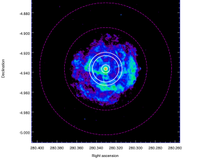
Figure 1: Chandra mosaic of SNR Kes 73. The solid white circles mark the three annular extraction regions for the SNR spectrum, at $r_{\rm int}^{\rm SNR}=6^{\prime\prime}$ (innermost circle, common to all three) and $r_{\rm ext}^{\rm SNR}=15^{\prime\prime}$, $48^{\prime\prime}$ and $60^{\prime\prime}$ (outer circles). The dashed magenta circles mark the extraction region used for the background of XMM-Newton, NuSTAR and IXPE data: $r_{\rm int}^{\rm bkg}=150^{\prime\prime}$ and $r_{\rm ext}^{\rm bkg}=240^{\prime\prime}$.

2.3 XMM-Newton

We analyzed the latest and deepest XMM-Newton observation of 1E 1841$-$045 (see Table 1). The analysis of this dataset is presented in this Letter for the first time. The European Photon Imaging Cameras (EPIC) instrument was operated in Prime Full Window (pn camera, Strüder et al. 2001) and Prime Partial Window (MOS1/2 cameras, Turner et al. 2001) with the thick filter.

Data reduction was performed using the epproc and emproc pipelines of version 18 of the Science Analysis System (SAS). The extraction regions for the source and background are shown in Figure 1. We selected single- and multiple-pixel events (pattern$\leq$4 for the EPIC-pn and $\leq$12 for the EPIC-MOS).

2.4 NuSTAR

NuSTAR (Harrison et al., 2013) observed 1E 1841$-$045 twice, following the recent bursting activity: the first observation started on August 29 and lasted $50\,\mathrm{ks}$; the second started on September 28 and lasted $56\,\mathrm{ks}$. Furthermore, to compare the properties of broadband emission before and after the bursting episode, we analyzed a long observation ($100\,\mathrm{ks}$) made in September 2013 (see Table 1). Data were processed using the nupipeline tool with default screening parameters, and spectra were extracted throughout the energy bandpass using nuproducts. The extraction regions for the source and background are shown in Figure 1.

3 Results

We converted the times of arrival of the photons to the Solar System barycenter using the Jet Propulsion Laboratory Development Ephemeris JPL DE430, with source coordinates $\mathrm{R.A.=18^{h}41^{m}19.34^{s}}$, $\mathrm{Dec.=-04^{\circ}56^{\prime}11.16^{\prime\prime}}$. Spectral and spectro-polarimetric analyses were performed using XSPEC (Arnaud, 1996, version 12.11.0). Absorption from the interstellar medium was accounted for using the tbabs models with cross sections and abundances from Wilms et al. (2000). The $\chi^{2}$ statistics was used to assess the goodness of the fits, and all reported errors are at $1\sigma$ confidence level (cl hereafter), unless otherwise specified.

3.1 Spectral analysis

3.1.1 Pre bursting activity

We simultaneously fit the XMM-Newton-EPIC and NuSTAR spectra of 1E 1841$-$045 obtained before the August 2024 bursting phase. The emission component of SNR Kes 73 was included as explained in §2.2, and we added a constant to account for the calibration uncertainties between the three EPIC cameras and the two NuSTAR modules.

We fitted to the spectra a (absorbed) two-component model, either two power laws (PL+PL), or a blackbody and a power law (BB+PL). In both cases, the fit was poor, with $\chi^{2}/\mathrm{dof}=3319.90/2671$ and $3331.42/2671$, respectively, with a structured modulation in the residuals, suggesting the presence of an additional component. We then added a BB as a third component, obtaining $\chi^{2}/\mathrm{dof}=2847.25/2669$ for the BB+PL+PL model and $\chi^{2}/\mathrm{dof}=2919.53/2669$ for the BB+BB+PL model (see the two panels in Figure 2 and Table 2). The addition of the third component yields in both cases an F-test probability $<$10^-16. The total unabsorbed fluxes in the $2$–$8\,\mathrm{keV}$ energy range turned out to be $F_{\mathrm{BB+PL+PL}}=(2.11\pm 0.01)\times 10^{-11}\,\mathrm{erg\,cm}^{-2}\mathrm{\,s}^{-1}$ and $F_{\mathrm{BB+BB+PL}}=(2.03\pm 0.01)\times 10^{-11}\,\mathrm{erg\,cm}^{-2}\mathrm{\,s}^{-1}$.

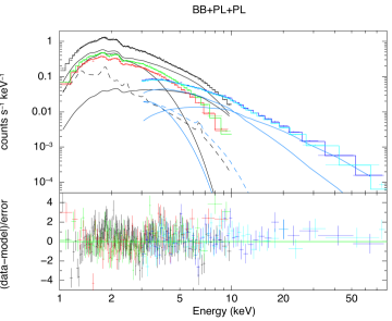
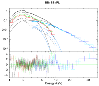
Figure 2: Best fit and residuals to the XMM-Newton (EPIC-pn in black, MOS1 and MOS2 in red and green respectively) and NuSTAR (FPMA and FPMB detectors in blue and cyan respectively) pre-burst data. The solid lines show the single components of the models, while the dashed lines show the SNR contribution as computed in §2.2, which was kept fixed in all fits. The plotted spectra were rebinned to improve visualization and single components are only displayed in the cases of the EPIC-pn and FPMA detectors for clarity.

3.1.2 Post bursting activity

We fit the simultaneous IXPE and NuSTAR spectra in the $2$–$79\,\mathrm{keV}$ energy range. A cross-calibration constant was introduced to account for the different response of the three IXPE DUs and the two NuSTAR modules; the contribution of SNR Kes 73 was included as explained in §2.2.

We started with absorbed PL+PL and BB+PL models and obtained best fits with $\chi^{2}/\mathrm{dof}=904.11/883$ and $972.07/883$, respectively. The PL+PL fit is formally acceptable, but yields a very high column absorption $N_{\mathrm{H}}=(4.4\pm 0.2)\times 10^{22}\,\mathrm{cm}^{-2}$ and an unreasonably steep photon index of $\Gamma_{1}=5.00\pm 0.14$, probably mimicking the presence of a thermal component.

As a consequence, following the approach discussed in 3.1.1, we considered a three-model spectral decomposition for the IXPE and NuSTAR data. Given the reduced energy band of IXPE and the lower number of source counts, we froze the value of the column density to those obtained in §3.1.1. We found that both the BB+PL+PL and BB+BB+PL decompositions provide an acceptable fit ($\chi^{2}/\mathrm{dof}=904.54/882$ and $900.77/882$, respectively) with an even distribution of the residuals and an improvement with respect to the BB+PL model (F-test probability $\sim 10^{-15}$). The data, together with the best-fit models, are shown in Figure 3, and the corresponding best-fit parameters are reported in Table 2. The unabsorbed fluxes in the $2$–$8\,\mathrm{keV}$ energy range are $F_{\mathrm{BB+PL+PL}}=(2.31\pm 0.02)\times 10^{-11}\,\mathrm{erg\,cm}^{-2}\mathrm{\,s}^{-1}$ and $F_{\mathrm{BB+BB+PL}}=(2.22\pm 0.02)\times 10^{-11}\,\mathrm{erg\,cm}^{-2}\mathrm{\,s}^{-1}$.

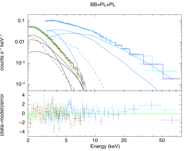
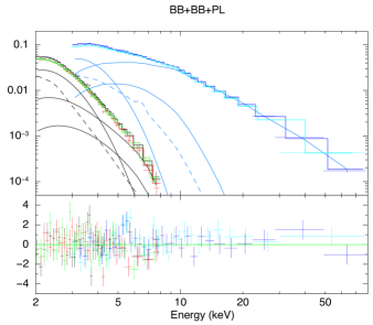
Figure 3: Best fit and residuals to the IXPE (DU1, DU2 and DU3 in black, red and green respectively) and NuSTAR (FPMA and FPMB detectors in blue and cyan respectively) 2024 data. Line code is as in Figure 2.

Table 2: Fit parameters of 1E 1841$-$045 spectra

	BB+PL+PL		BB+BB+PL
	PRE	POST	PRE	POST
$N_{\mathrm{H}}$ ($10^{22}\,\mathrm{cm}^{-2}$)	$2.20_{-0.03}^{+0.03}$	$2.20^{*}$	$2.009_{-0.014}^{+0.015}$	$2.009^{*}$
$kT_{\mathrm{BB}_{1}}$ (keV)	$0.491_{-0.004}^{+0.004}$	$0.501_{-0.007}^{+0.007}$	$0.465_{-0.008}^{+0.007}$	$0.524_{-0.008}^{+0.008}$
$R_{\mathrm{BB}_{1}}$ (km)	$3.94_{-0.13}^{+0.12}$	$4.62_{-0.23}^{+0.23}$	$5.58_{-0.15}^{+0.18}$	$4.65_{-0.15}^{+0.16}$
$F_{\mathrm{BB_{1}}}^{2-8}$ ($10^{-12}\,\mathrm{erg\,cm}^{-2}\mathrm{\,s}^{-1}$)	$5.25_{-0.25}^{+0.24}$	$8.2_{-0.6}^{+0.5}$	$7.6_{-0.4}^{+0.3}$	$10.6_{-0.3}^{+0.3}$
$kT_{\mathrm{BB}_{2}}$ (keV)	–	–	$1.04_{-0.05}^{+0.05}$	$1.4_{-0.1}^{+0.1}$
$R_{\mathrm{BB}_{2}}$ (km)	–	–	$0.56_{-0.06}^{+0.07}$	$0.24_{-0.03}^{+0.04}$
$F_{\mathrm{BB_{2}}}^{2-8}$ ($10^{-12}\,\mathrm{erg\,cm}^{-2}\mathrm{\,s}^{-1}$)	–	–	$4.3_{-0.2}^{+0.2}$	$2.6_{-0.3}^{+0.3}$
$\Gamma_{\mathrm{PL_{2}}}$	$2.5_{-0.1}^{+0.1}$	$2.4_{-0.3}^{+0.2}$	–	–
$F_{\mathrm{PL_{2}}}^{2-8}$ ($10^{-12}\,\mathrm{erg\,cm}^{-2}\mathrm{\,s}^{-1}$)	$12.2_{-0.4}^{+0.4}$	$9.3_{-0.9}^{+0.8}$	–	–
$\Gamma_{\mathrm{PL_{3}}}$	$0.93_{-0.07}^{+0.06}$	$1.1_{-0.07}^{+0.06}$	$1.34_{-0.02}^{+0.02}$	$1.30_{-0.03}^{+0.03}$
$F_{\mathrm{PL_{3}}}^{2-8}$ ($10^{-12}\,\mathrm{erg\,cm}^{-2}\mathrm{\,s}^{-1}$)	$3.3_{-0.5}^{+0.6}$	$5.7_{-1.7}^{+1.1}$	$8.4_{-0.3}^{+0.3}$	$9.0_{-0.4}^{+0.4}$
$F_{\mathrm{TOT}}^{2-8}$ ($10^{-12}\,\mathrm{erg\,cm}^{-2}\mathrm{\,s}^{-1}$)	$21.1_{-0.1}^{+0.1}$	$23.1_{-0.2}^{+0.2}$	$20.3_{-0.1}^{+0.1}$	$22.2_{-0.2}^{+0.2}$
$F_{\mathrm{TOT}}^{8-79}$ ($10^{-12}\,\mathrm{erg\,cm}^{-2}\mathrm{\,s}^{-1}$)	$54.3_{-0.7}^{+0.7}$	$59_{-1}^{+1}$	$50.0_{-0.7}^{+0.7}$	$58_{-1}^{+1}$
$K_{\rm pn}$/$K_{\rm DU1}$	$1^{*}$	$1^{*}$	$1^{*}$	$1^{*}$
$K_{\rm MOS1}$/$K_{\rm DU2}$	$1.139\pm 0.005$	$0.972\pm 0.011$	$1.139\pm 0.005$	$0.971\pm 0.011$
$K_{\rm MOS2}$/$K_{\rm DU3}$	$1.061\pm 0.005$	$0.978\pm 0.011$	$1.061\pm 0.005$	$0.978\pm 0.011$
$K_{\rm FMPA}$	$1.185\pm 0.007$	$1.328\pm 0.017$	$1.183\pm 0.007$	$1.326\pm 0.017$
$K_{\rm FMPB}$	$1.147\pm 0.007$	$1.314\pm 0.017$	$1.143\pm 0.007$	$1.312\pm 0.017$
$\chi^{2}/\mathrm{dof}$	2847.25/2669	904.54/882	2919.53/2669	900.77/882

3.2 Polarization analysis

3.2.1 Energy-resolved polarimetric analysis

The phase-averaged Stokes parameters $I$, $Q$ and $U$ integrated over the $2$–$8\,\mathrm{keV}$ band were obtained from the photon lists for each of the IXPE DUs using the ixpeobssim package Baldini et al. (2022). The results for the normalized Stokes parameters $Q/I$ and $U/I$ are shown in Figure 4. The detection obtained from the sum of the three DUs is highly significant ($\gtrsim 8\sigma$), yielding a polarization degree $\mathrm{PD}=\sqrt{Q^{2}+U^{2}}/I=25.9\pm 3.1\%$, well above the minimum detectable polarization at $99\%$ cl ($\mathrm{MDP}_{99}$, see Weisskopf et al., 2010) of $9.5\%$, and a polarization angle $\mathrm{PA}=\arctan{(U/Q)}/2=1.1\pm 3.5^{\circ}$, measured east of celestial north.

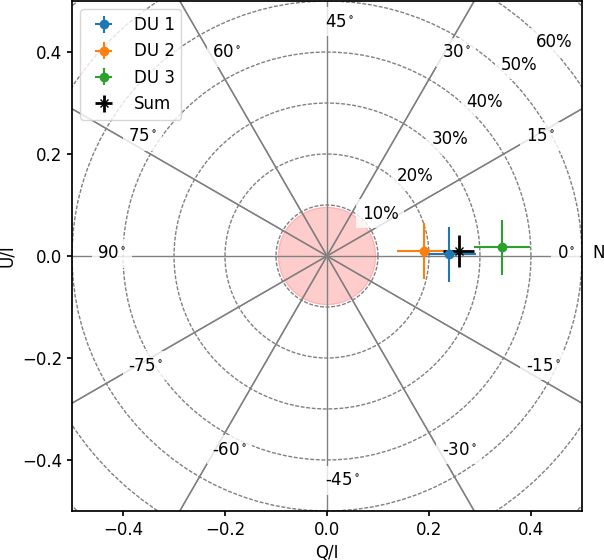
Figure 4: The normalized Stokes parameters $Q/I$ and $U/I$ measured by the IXPE DU1 (cyan), DU2 (orange) and DU3 (green) along with the combined measurements from the three DUs (black); $1\sigma$ error bars are also shown. Dashed circles represent the loci of constant $\mathrm{PD}$ while straight lines those of constant $\mathrm{PA}$. The $\mathrm{MDP}_{99}$ relative to the combined measurement is marked by the filled circle.

We then divided the $2$–$8\,\mathrm{keV}$ energy band into four energy bins and extracted the values of $\mathrm{PD}$ and $\mathrm{PA}$ in each of them. Polarization properties were derived using both the pcube algorithm within the ixpeobssim suite and by fitting simultaneously the $I$, $Q$ and $U$ spectra with XSPEC in each energy interval. In the latter case, we first fit the IXPE spectrum (Stokes $I$) in the $2$–$8\,\mathrm{keV}$ band using a simple BB+PL model with $N_{\mathrm{H}}$ frozen at the value listed in Table 2 ($\chi^{2}/\mathrm{dof}=230.95/216$). Then, we fit simultaneously the spectra of $I$, $U$, and $Q$ in each energy interval, keeping the parameters of BB and PL at their best-fit values found previously, and convolving the spectral model with a constant polarization (polconst).

The results, reported in Table 3, show an overall agreement (within $1\sigma$) between the parameters obtained using the two methods, confirming a posteriori that the method used to extract $\mathrm{PD}$ and $\mathrm{PA}$ with XSPEC is essentially model independent. The measurements are above $\mathrm{MDP}_{99}$ in each energy bin, with significance $>3\sigma$. The most probable values of $\mathrm{PD}$ and $\mathrm{PA}$, together with the corresponding confidence contours at $68\%$ and $99\%$ cl, are also plotted in Figure 5. The degree of polarization increases monotonically with energy, from $\approx 15\%$ at $2$–$3\,\mathrm{keV}$ up to more than $50\%$ at higher energies ($5.5$–$8\,\mathrm{keV}$), while the polarization angle remains fairly constant, with only a slight deviation in the bin at the highest energy. However, the polarization direction is compatible with that of the celestial north in the entire IXPE band within $1\sigma$.

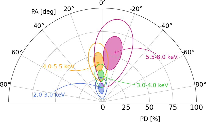
Figure 5: Polar plot of the energy-dependent PD and PA obtained using XSPEC (see text for details). Filled and empty contours correspond to the $68\%$ and $99\%$ confidence regions, respectively, around the most probable values reported in Table 3.

Table 3: Energy-resolved polarization degree and angle

	$2.0$–$3.0\,\mathrm{keV}$	$3.0$–$4.0\,\mathrm{keV}$	$4.0$–$5.5\,\mathrm{keV}$	$5.5$–$8.0\,\mathrm{keV}$	$2.0$–$8.0\,\mathrm{keV}$
pcube PD ($\%$)	$16.1\pm 3.5$	$28.0\pm 4.0$	$37.9\pm 6.1$	$54.2\pm 15.2$	$25.8\pm 3.1$
pcube PA (deg)	$4.6\pm 6.3$	$2.1\pm 4.1$	$2.0\pm 4.6$	$-6.7\pm 8.0$	$1.1\pm 3.5$
pcube PD S/N	$4.6\sigma$	$7.0\sigma$	$6.2\sigma$	$3.6\sigma$	$8.3\sigma$
pcube $\mathrm{MDP}_{99}$ ($\%$)	$10.7$	$12.1$	$18.5$	$45.9$	$9.5$
XSPEC PD ($\%$)	$14.5\pm 3.8$	$27.9\pm 4.1$	$43.1\pm 6.6$	$52.9\pm 12.1$	$25.3\pm 2.4$
XSPEC PA (deg)	$3.3\pm 7.5$	$1.7\pm 4.2$	$4.1\pm 4.4$	$-12.9\pm 6.7$	$2.3\pm 2.7$
XSPEC PD S/N	$3.8\sigma$	$6.8\sigma$	$6.5\sigma$	$4.4\sigma$	$10.5\sigma$

3.2.2 Phase-resolved polarimetric analysis

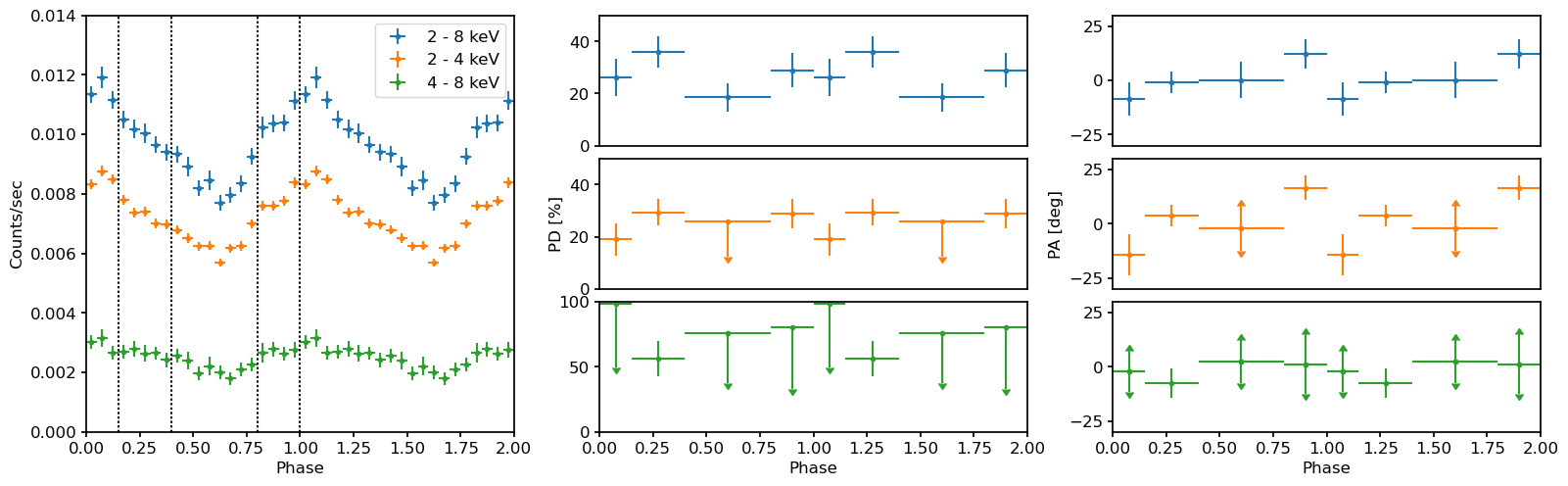
Figure 6: IXPE count rate (left panel), polarization degree (central panel) and polarization angle (right panel) as a function of the rotational phase; two cycles are shown for clarity. Results are presented for the $2$–$8$ (blue), $2$–$4$ (orange) and $4$–$8\,\mathrm{keV}$ (green) energy ranges. Polarization degree and angle are shown for the four phase intervals marked by vertical dotted lines in the left panel. In all the bins where PD is below $\mathrm{MDP}_{99}$, a $3\sigma$ upper limit (marked by a downward arrow) is shown for PD and the errors on PA are extended over the entire $[-90^{\circ}$, $90^{\circ}]$ range (double-headed arrows).

To perform a phase-dependent polarimetric analysis, we measured the spin period of 1E 1841$-$045 at the epoch of the IXPE observation. We extracted the period by searching around the frequency $0.085\,\mathrm{Hz}$ reported in Dib & Kaspi (2014) and using the $Z_{n}^{2}$-search technique included in the HENDRICS suite v.7.0 Bachetti (2018). We found that the most likely value for the frequency is $f=0.08469848(8)\,\mathrm{Hz}$, corresponding to a period $P=11.80659(1)\,\mathrm{s}$, at the MJD epoch $60587.140813793325$, while the value of the frequency derivative was not constrained.

The pulse profile shown in the left panel of Figure 6 is obtained folding the data at our best spin period and dividing the counts into $20$ equally spaced bins. The pulse shape and the pulsed fraction do not appear to change significantly with energy, with the latter being $(21.2\pm 1.5)\%$ in the $2$–$4\,\mathrm{keV}$ band and only slightly higher (but still compatible within $1\sigma$) in the $4$–$8\,\mathrm{keV}$ range, $(27.6\pm 7.3)\%$.

Subsequently, we considered $4$ phase intervals, corresponding to the peak, decline, dip, and rise of the pulse, to obtain a significant detection ($\mathrm{PD}>\mathrm{MDP}_{99}$) in each bin (see again the left panel of Figure 6). The results for $\mathrm{PD}$ and $\mathrm{PA}$, obtained using the ixpeobssim-pcube algorithm, are shown in Figure 6 (center and right panels) and reported in Table 4. In the $2$–$8\,\mathrm{keV}$ range, the polarization degree varies between $\approx 20\%$ and $36\%$. A fit with a simple sinusoidal profile of both counts and $\mathrm{PD}$ is acceptable at better than $99\%$ cl, and suggests that the two oscillations are in-phase within $1\sigma$ errors, although the polarization degree is compatible with a constant within $2\sigma$.

We also analyzed the phase-dependent behavior of the polarization in the $2$–$4$ and $4$–$8\,\mathrm{keV}$ energy ranges. At lower energies, the degree of polarization is above $\mathrm{MDP}_{99}$ in three phase bins and slightly below around the pulse minimum. Either considering only the three secure measurements or assigning to $\mathrm{PD}$ at the dip its most probable value, the polarization degree turns out to be incompatible with a constant (at $99\%$ cl), and a fit with a sinusoidal profile is still in-phase with the lightcurve. At higher energies ($4$–$8\,\mathrm{keV}$), the polarization signal is significant in only one out of four phase intervals, barring any firm conclusions.

A fit of the polarization angle, following the same procedure discussed above, shows that $\mathrm{PA}$ is compatible with a constant in the $2$–$8\,\mathrm{keV}$ range but not in the soft $2$–$4\,\mathrm{keV}$ energy band. We also tested the rotating vector model (RVM, see Radhakrishnan & Cooke, 1969), in analogy to what was done in other magnetar sources (see Taverna et al., 2022; Zane et al., 2023; Heyl et al., 2024) and X-ray pulsars Poutanen et al. (2024). However, the fit turned out to be quite poor, with the two-model parameters, i.e. the inclinations of the line-of-sight and magnetic axis with respect to the rotation axis, being totally unconstrained.

Table 4: Phase-resolved polarization degree and angle.

Phase bin	Energy range	PD	PA	PD S/N
	(keV)	($\%$)	(deg)
	$2.0-8.0$	$26.1\pm 7.1$	$-8.5\pm 7.8$	$3.7\sigma$
$0.0-0.15$	$2.0-4.0$	$19.0\pm 6.3$	$-14.3\pm 9.4$	$3.0\sigma$
	$4.0-8.0$	$<98.7$	-	-
	$2.0-8.0$	$35.8\pm 6.0$	$-0.9\pm 4.8$	$6.0\sigma$
$0.15-0.4$	$2.0-4.0$	$29.4\pm 5.3$	$3.7\pm 5.1$	$5.6\sigma$
	$4.0-8.0$	$56.1\pm 13.6$	$-7.5\pm 6.9$	$4.1\sigma$
	$2.0-8.0$	$18.5\pm 5.5$	$0.2\pm 8.4$	$3.4\sigma$
$0.4-0.8$	$2.0-4.0$	$<25.7$	-	-
	$4.0-8.0$	$<76.2$	-	-
	$2.0-8.0$	$29.0\pm 6.8$	$12.2\pm 6.7$	$4.3\sigma$
$0.8-1.0$	$2.0-4.0$	$28.9\pm 5.7$	$16.5\pm 5.6$	$5.1\sigma$
	$4.0-8.0$	$<80.1$	-	-

3.2.3 Spectro-polarimetric analysis

As a final step, we explored the polarization properties of the individual components entering the spectral models discussed in §3.1, i.e. tbabs $\times$ $($snr $+$ bbodyrad $+$ bbodyrad $+$ powerlaw$)$ (hereafter model 1) and tbabs $\times$ $($snr $+$ bbodyrad $+$ powerlaw $+$ powerlaw$)$ (hereafter model 2), where snr stands for the SNR spectral model discussed in §2.2. We froze all spectral parameters at the values reported in Table 2 (POST) and convolved each spectral component with a constant polarization model (polconst), simultaneously fitting the $I$, $Q$ and $U$ spectra.

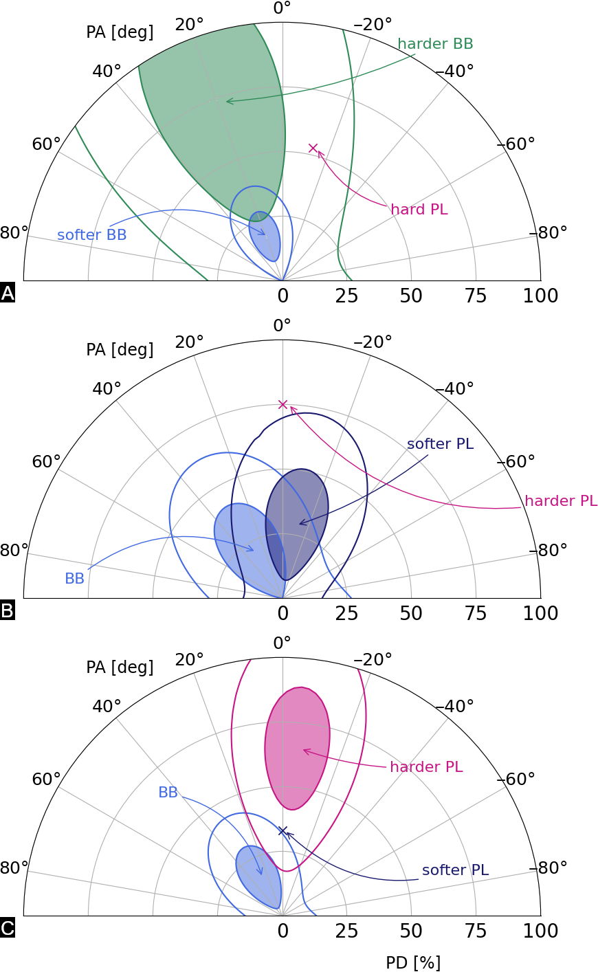
Figure 7: Polarization of the single spectral components (see text for details). Filled and empty contours correspond to the $68\%$ and $99\%$ confidence regions, respectively, around the most probable values; crosses mark the values at which $\mathrm{PD}$ and $\mathrm{PA}$ were frozen for the specified component.

Although the contribution of the SNR to the flux is sizable at $2$–$4\,\mathrm{keV}$ (see Figure 3 and Table A1), its polarization is expected to be small, as discussed at the end of the section. Consequently, we froze the SNR polarization degree to zero.

The hard PL accounts for almost all the counts above $\approx 5\,\mathrm{keV}$ in the case of model 1 (see Figure 3, right panel). Therefore, we fixed its polarization to the value measured with IXPE in the $5.5$–$8\,\mathrm{keV}$ range (see Table 3) and allowed the polarization of the soft and hard BBs to vary. As shown in Figure 7 (panel A), the polarization of the softer thermal component is approximately $20\%$ and is constrained at $99\%$ cl, while that of the hot blackbody is unconstrained, and we can only conclude that the two thermal components are polarized in the same direction at a confidence level of $68\%$.

On the other hand, in model 2 no single component dominates the spectrum in any energy range (see Figure 3, left panel). So, none of them can be associated a priori with the polarization measured by IXPE in a given energy interval. Since a fit with all parameters left free is particularly poor, with all the parameters unconstrained, we decided to run different tests, allowing the fit to compute the polarization of two components and freezing that of the third one.

First, we checked that, by freezing only the degree of polarization of one of the three components and leaving all other polarization parameters free to vary, the polarization of the other two components is unconstrained at $68\%$. Then, for the component with frozen polarization, we fixed both $\mathrm{PD}$ and $\mathrm{PA}$. In particular, we decided to take $\mathrm{PA}=0^{\circ}$, in agreement, within $1\sigma$ cl, with the IXPE measurement in all the energy bins (see Figure 5).

The high polarization degree obtained in the $2$–$8\,\mathrm{keV}$ energy interval suggests that, in the case of model 1, the hard PL component may be due to synchrotron radiation. Hence, for model 2 we fixed the $\mathrm{PD}$ of the hard PL, taking $75\%$ as representative of synchrotron emission (see e.g. Rybicki & Lightman, 1979). Note that this is not the PD measured in the $5.5$–$8\,\mathrm{keV}$ bin, since both PLs contribute in this energy range, allowing the soft PL to be less polarized. The result is reported in panel B of Figure 7. Although the polarization of both components turns out to be unconstrained at $99\%$ cl, the derived values at $68\%$ cl are $\approx 20\%$ for the BB and $\approx 30\%$ for the soft PL, while $\mathrm{PA}$ is compatible with zero, in agreement with observations. The latter value of $\mathrm{PD}$ suggests that the soft PL may be produced by resonant Compton scattering (RCS, which predicts $\mathrm{PD}\approx 33\%$; Taverna et al., 2020). We then froze this parameter at $33\%$, imposing again $\mathrm{PA}=0^{\circ}$, and leaving the polarization of the BB and the hard PL free to vary. The result is reported in Figure 7 (panel C). In this case, the degree of polarization of the hard PL is well constrained at $\mathrm{PD}\approx 65\%$ and its polarization angle is $\mathrm{PA}\approx-6^{\circ}$ (and compatible with $0^{\circ}$ within $1\sigma$). This suggests that, under the assumption that the polarization of each spectral component is constant across the IXPE band, the data can be reproduced by a model comprising a soft BB with $\mathrm{PD}\approx 20\%$, a mildly polarized soft PL ($\mathrm{PD}\approx 30\%$) and a highly polarized hard PL, all with a polarization direction compatible with $0^{\circ}$.

Finally, we checked that by extracting the IXPE counts in an annular region centered on the source, with inner and outer radii $30^{\prime\prime}$ and $150^{\prime\prime}$, respectively, from which the background was subtracted as described above, the pcube PD turns out to be below $\mathrm{MDP}_{99}\approx 20\%$, both in the $2$–$8\,\mathrm{keV}$ and in the $2$–$4\,\mathrm{keV}$ energy ranges. This supports the assumption that SNR emission exhibits relatively low polarization, consistent with other SNRs observed by IXPE, where the average degree of polarization does not exceed $\approx$10% at most (see e.g. Slane et al., 2024). As a further test, we performed the fit with model 2 under the same conditions discussed above, but considering the polarization angle frozen at $+90^{\circ}$ or $-90^{\circ}$. This resulted in a $>100\%$ polarization of at least one of the two free components, and thus reasonably rules out the possibility that the emission associated with a specific spectral component is polarized perpendicularly to that associated with the other two.

4 Discussion

In this work, we investigated the spectro-polarimetric properties of 1E 1841$-$045 after it entered a period of bursting activity. We found that the emission over the whole IXPE energy band is strongly polarized, with $\mathrm{PD}=(25.9\pm 3.1)\%$ and $\mathrm{PA}=(1.1\pm 3.5)^{\circ}$ at a significance greater than $8\sigma$. The degree of polarization increases monotonically with energy, and its variation with the rotational phase broadly follows the pulse profile. The polarization angle remains fairly constant in both energy and phase, with the exception of the $2$–$4\,\mathrm{keV}$ energy range, where a phase modulation in $\mathrm{PA}$ is detected.

The broadband ($2$–$79\,\mathrm{keV}$) spectrum, obtained joining IXPE and simultaneous NuSTAR data, can be reproduced equally well by a BB+PL+PL or BB+BB+PL model. The $2$–$8\,\mathrm{keV}$ fluxes are about 10% higher than those obtained with the same spectral decompositions from archival XMM-Newton and NuSTAR data collected before the bursting phase. The increase in flux is more pronounced (about $15\%$) at higher energies, between $8$ and $79\,\mathrm{keV}$.

There is no substantial evolution of the spectral parameters with respect to the pre-burst state, although the temperature (radius) of the hotter BB increased (decreased) after the onset of the bursting activity. No evidence of a further hot and bright thermal component associated with a large heat deposition in the crust was found, as instead observed in full-fledged outbursts (see e.g. Coti Zelati et al., 2018).

However, a significant evolution is seen in the pulse profile. We found the best-folding spin period in each of the XMM-Newton and NuSTAR observations (see Table 1) and we obtained the pulse profiles shown in Figure 8. Before the burst, the 2017 EPIC-pn and the 2013 NuSTAR data (first and second panels in Figure 8) consistently show a double-peaked profile, with $\mathrm{PF}=(23.6\pm 0.9)\%$ at $2$–$8\,\mathrm{keV}$ and $(25.2\pm 1.6)\%$ at $8$–$79\,\mathrm{keV}$. In the NuSTAR data obtained a few days after the burst-active phase onset, a dip appeared in the rise toward the primary peak (third panel, see also Younes et al. 2024) that partially recovered one month later (fourth panel). The pulse profile measured by IXPE (see Figure 6, left panel) reveals the presence of two plateaux, just before and after the main peak, which are reminiscent of the secondary peak and the small dip seen in the NuSTAR 2024 data (fourth panel in Figure 8). These features are not well resolved in the IXPE light curve, likely due to the lower number of events collected in the relatively short exposure time. The pulsed fraction attains a value quite similar to that of the other instruments, with $\mathrm{PF}=(21.5\pm 2.2)\%$ in the $2$–$8\,\mathrm{keV}$ band, without significant changes with energy.

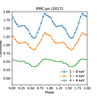
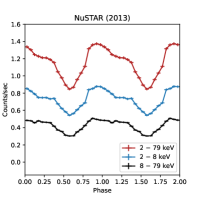
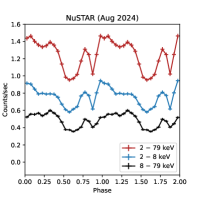
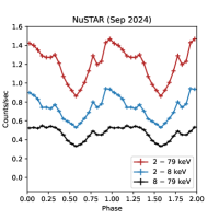
Figure 8: Background-subtracted EPIC-pn pulse profiles in the $2$–$8$ (blue), $2$–$4$ (orange) and $4$–$8\,\mathrm{keV}$ (green) energy bands (left panel). The three rightmost panels show the NuSTAR pulse profiles in the $2$–$79$ (red), $2$–$8$ (blue) and $8$–$79\,\mathrm{keV}$ (black) energy bands at three different epochs.

Like other magnetars, 1E 1841$-$045 is known to exhibit significant hard X-ray emission. These high-energy tails were originally detected by INTEGRAL (Kuiper et al., 2004, 2006; Mereghetti et al., 2005; Molkov et al., 2005; Götz et al., 2006), can extend up to a few hundreds of keV, and are highly phase dependent (den Hartog et al., 2008a, b; Vogel et al., 2014; Yang et al., 2016). Their physical origin is still poorly understood and different interpretations have been proposed, ranging from thermal bremsstrahlung in the surface layers heated by returning currents, to synchrotron emission from pairs in the magnetosphere (Thompson & Beloborodov, 2005), to Compton resonant upscattering from relativistic charges (Baring et al., 2005; Baring & Harding, 2008; Beloborodov, 2013; Wadiasingh et al., 2018). Thanks to NuSTAR, we were able to characterize this emission component after the beginning of the burst-active phase. We find that the hard power law contributes significantly to the large polarization of the source at higher energies ($5$–$8\,\mathrm{keV}$).

Attempts to perform a spectro-polarimetric analysis of the IXPE data alone by associating a constant polarization model to each spectral component and leaving all parameters free to vary resulted in a largely unconstrained fit. However, fixing the polarization parameters of one of the spectral components produces a reasonably constrained fit, and the hard PL turns out to be polarized at more than $65\%$, regardless of which component is actually frozen. This large polarization is difficult to reconcile with resonant Compton scattering models, which predict $\mathrm{PD}\approx 30\%$–$40\%$ because of the $1/3$ ratio of the X- and O-mode photon scattering cross sections (Fernández & Davis, 2011; Taverna et al., 2014; Wadiasingh et al., 2018, see also Stewart et al. 2025). On the other hand, the derived polarization degree and the power-law spectral distribution point to a synchrotron/curvature origin for the high-energy tail (see e.g. Bandiera & Petruk, 2024). If one assumes that synchrotron radiation is produced by a power-law distribution of electrons, the photon index $\Gamma_{\mathrm{PL}_{3}}\approx 1$, inferred from the spectral fit with the BB+BB+PL model (see Table 2 POST), implies a degree of polarization of $\approx 75\%$ Rybicki & Lightman (1979). Interestingly, by fixing the polarization degree of the hard PL at $75\%$, the soft PL turned out to be polarized at around $30\%$, as expected if it is produced by resonant Compton scattering in the star magnetosphere (see Taverna et al., 2014, 2020). Moreover, the polarization of the soft thermal component is $\approx 25\%$, close to that observed in other magnetars Taverna et al. (2022); Zane et al. (2023); Heyl et al. (2024). Such polarization can hardly come from a strongly magnetized, passive atmosphere ($B\gtrsim 10^{14}\,\mathrm{G}$, also allowing for mode conversion; Kelly et al., 2024b), while it may be produced by a condensed surface or a bombarded atmosphere Taverna et al. (2020); Kelly et al. (2024a).

Although the presence of a soft, thermal, mildly polarized component and a hard, strongly polarized power law appears to be well established, the nature of emission at intermediate energies ($\approx 3$–$6\,\mathrm{keV}$) is not so clear. It could be either a softer power law, due to the RCS of the seed thermal photons, or a second, hotter thermal component. In the latter case, the relatively large polarization ($\approx 30\%$) is incompatible with emission from a condensed surface and suggests that part of the star is covered by an atmosphere, as proposed for 1RXS J1708 (Zane et al., 2023).

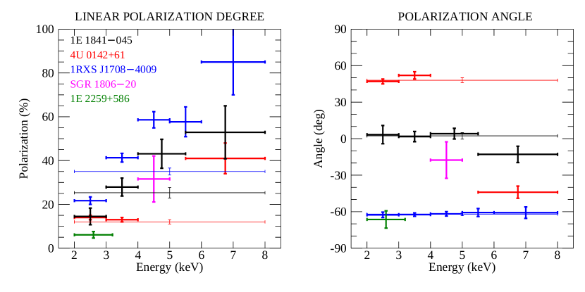
Figure 9: Energy dependence of the linear polarization degree (left panel) and polarization angle (right panel) of the five magnetars observed with IXPE. Thin lines indicate results for the total energy range (in case of significant polarization detection in the $2$–$8\,\mathrm{keV}$ range). See details in Taverna et al. (2022); Zane et al. (2023); Turolla et al. (2023); Heyl et al. (2024).

In 1E 1841$-$045 the polarization direction appears to change little with energy, implying that the two lower energy components are polarized in the same mode, in the O- or X-mode. Although there is no way to determine which is the dominant polarization mode from the data, in respect to the intermediate component, we note that both atmospheric emission (if the preferred model is BB+BB+PL) and RCS (in case of the BB+PL+PL decomposition) produce radiation which is mostly polarized in the X mode. This lends support to the soft BB being polarized in the X mode, too. In fact, the emission of a magnetic condensate can be polarized either in the X- or O-mode, depending on the emission/viewing geometry, and polarization in the X-mode has been invoked for the thermal component in 1RXS J1708. The observed agreement of the polarization direction of the hard PL photons with those of the two other spectral components is intriguing, given that synchrotron emission is polarized perpendicular to the magnetic field projection in the plane of the sky and is not, in general, associated with the X- and O-modes. However, if synchrotron radiation comes from below the polarization-limiting radius (located at $\approx 100\,R_{NS}$, see e.g. Taverna et al., 2015), the strong $B$-field will force also synchrotron photons to propagate in the two normal modes, likely in the X-mode for the case at hand. This scenario is compatible with synchrotron emission due to a population of relativistic pairs near the footprints of the field lines, as suggested by Beloborodov (2013).

The general behavior of the polarization in 1E 1841$-$045 (monotonic increase with energy of $\mathrm{PD}$ at a constant polarization angle) is reminiscent of that observed in 1RXS J1708. The similarity between the two sources goes deeper, since both exhibit a double power-law tail with comparable spectral indices ($\Gamma_{\mathrm{soft}}\sim 2.5$–$2.7$ and $\Gamma_{\mathrm{hard}}\sim 1$; see den Hartog et al., 2008a, for the X-ray spectrum of 1RXS J1708). Zane et al. (2023) proposed two possible scenarios for 1RXS J1708: either two thermal components, one with low polarization and the other with high polarization, or one thermal component polarized at $\approx 20\%$ and a power law, with $\Gamma\sim 3$, polarized at $\approx 70\%$. According to the latter interpretation, the same scenario discussed here for 1E 1841$-$045 may also apply to 1RXS J1708, although the lack of simultaneous high-energy observations prevented in their case the complete characterization of the spectro-polarimetric properties at the upper end of the IXPE energy range.

5 Conclusions

We have reported the first X-ray polarimetric measurements of the magnetar 1E 1841$-$045 obtained with the IXPE satellite, together with a detailed analysis of data from Chandra, XMM-Newton and NuSTAR. These complementary data have been essential to properly take into account the non-negligible contribution of the Kes 73 SNR (20% of the $2$–$8\,\mathrm{keV}$ flux in the IXPE source extraction region) and to place the observed broadband flux and spectral properties of 1E 1841$-$045 in the context of the previous history of this persistent magnetar. In fact, the IXPE observation was obtained 40 days after the period of bursting activity and increased persistent flux that occurred in August 2024.

The polarization properties found for 1E 1841$-$045 are compared to those of the other four magnetars observed with IXPE in Figure 9. Similarly to 1RXS J1708, the linear polarization increases with energy from $\sim 15\%$ to $\sim 55\%$, without any change in the polarization angle.

We found that a three-component spectral model (either BB+PL+PL or BB+BB+PL) is required to fit the simultaneous IXPE and NuSTAR data, yielding a flux of $8\times 10^{-11}\,\mathrm{erg\,cm}^{-2}\mathrm{\,s}^{-1}$ between $2$–$79\,\mathrm{keV}$. The analysis of the archival XMM-Newton and NuSTAR data obtained before the source activation favors a BB+PL+PL model with flux of $7.5\times 10^{-11}\,\mathrm{erg\,cm}^{-2}\mathrm{\,s}^{-1}$ ($2$–$79\,\mathrm{keV}$, see also An et al. 2013). Although only a moderate increase of the flux was found between the pre- and the post-burst phases, the pulse profile experienced a noticeable evolution, especially above $8\,\mathrm{keV}$ where the hard power law dominates the flux.

High-energy tails are pretty ubiquitous in the magnetar population, but their origin is still poorly understood. Our spectro-polarimetric analysis showed that in 1E 1841$-$045  this component is polarized at more than $65\%$ and can be well interpreted in terms of synchrotron/curvature emission. The intermediate power-law component has a polarization degree of $30\%$, consistent with the predictions for resonant Compton scattering in the magnetosphere, while the moderate polarization of the soft, thermal component ($\approx 25\%$) may be produced by a condensed surface.

Future polarimetric missions in hard X-rays (like PHEMTO and ASTROMEV; Laurent et al., 2021; De Angelis et al., 2021) will prove key in assessing the synchrotron/curvature origin of magnetar hard tails and shed light on the nature of the other spectral components.

Appendix A SNR Kes 73

We report here the results of the spectral fit to the Chandra data of SNR Kes 73 (see §2.2 for details). The best fit parameters are listed in Table A1; the spectrum together with the best-fit model is shown in Figure A1.

Table A1: Fit parameters of SNR Kes 73 spectra

	SNR $6^{\prime\prime}-15^{\prime\prime}$	SNR $6^{\prime\prime}-48^{\prime\prime}$	SNR $6^{\prime\prime}-60^{\prime\prime}$
$N_{\mathrm{H}}$ ($10^{22}\,\mathrm{cm}^{-2}$)	$2.31_{-0.05}^{+0.06}$	$2.26_{-0.04}^{+0.06}$	$2.32_{-0.03}^{+0.02}$
$kT_{s}$ (keV)	$0.61_{-0.04}^{+0.05}$	$0.52_{-0.03}^{+0.05}$	$0.49_{-0.01}^{+0.02}$
$\tau_{s}$ ($10^{10}\,\mathrm{cm}^{-3}\,\mathrm{s}$)	$0.15_{-0.08}^{+0.07}$	$0.12_{-0.02}^{+0.02}$	$0.14_{-0.01}^{+0.02}$
$F_{s}^{2-8}$ ($10^{-12}\,\mathrm{erg\,cm}^{-2}\mathrm{\,s}^{-1}$)	$0.25_{-0.02}^{+0.02}$	$1.21_{-0.06}^{+0.14}$	$1.72_{-0.08}^{+0.06}$
$kT_{h}$ (keV)	$3.2_{-0.2}^{+0.2}$	$2.04_{-0.12}^{+0.04}$	$1.79_{-0.02}^{+0.04}$
$\tau_{h}$ ($10^{10}\,\mathrm{cm}^{-3}\,\mathrm{s}$)	$3.9_{-0.4}^{+0.4}$	$4.3_{-0.2}^{+0.3}$	$4.9_{-0.2}^{+0.2}$
$F_{h}^{2-8}$ ($10^{-12}\,\mathrm{erg\,cm}^{-2}\mathrm{\,s}^{-1}$)	$0.68_{-0.03}^{+0.03}$	$3.67_{-0.12}^{+0.08}$	$5.67_{-0.04}^{+0.18}$
Mg	$1^{*}$	$1.38_{-0.10}^{+0.06}$	$1.35_{-0.05}^{+0.05}$
Si	$1^{*}$	$1.58_{-0.07}^{+0.05}$	$1.61_{-0.05}^{+0.05}$
S	$1^{*}$	$2.01_{-0.11}^{+0.08}$	$2.05_{-0.08}^{+0.08}$
$K$	1.19048	1.01587	1.01010
$F_{\rm TOT}^{2-8}$ ($10^{-12}\,\mathrm{erg\,cm}^{-2}\mathrm{\,s}^{-1}$)	$1.11_{-0.02}^{+0.02}$	$4.98_{-0.03}^{+0.04}$	$7.47_{-0.04}^{+0.05}$
$\chi^{2}/\mathrm{dof}$	495.45/475	1537.00/1251	1813.83/1411

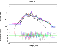
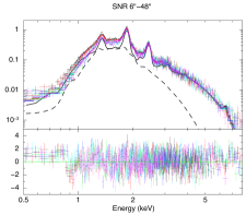
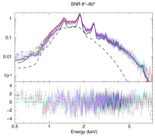
Figure A1: Best fit and residuals to the Chandra spectra of the SNR Kes 73. The three panels show the results for three annular extraction regions centered at (but excluding) 1E 1841$-$045, as detailed in §2.2. The six observations, displayed in black, red, green, blue, cyan and magenta in increasing order of date, were jointly fit with two vpshock components, shown as a solid (hot component) and dashed (soft component) black lines.

References

- An et al. (2013) An, H., Hascoët, R., Kaspi, V. M., et al. 2013, ApJ, 779, 163, doi: 10.1088/0004-637X/779/2/163
- Anders & Grevesse (1989) Anders, E., & Grevesse, N. 1989, Geochim. Cosmochim. Acta, 53, 197, doi: 10.1016/0016-7037(89)90286-X
- Arnaud (1996) Arnaud, K. A. 1996, in Astronomical Society of the Pacific Conference Series, Vol. 101, Astronomical Data Analysis Software and Systems V, ed. G. H. Jacoby & J. Barnes, 17
- Astropy Collaboration et al. (2013) Astropy Collaboration, Robitaille, T. P., Tollerud, E. J., et al. 2013, A&A, 558, A33, doi: 10.1051/0004-6361/201322068
- Astropy Collaboration et al. (2018) Astropy Collaboration, Price-Whelan, A. M., Sipőcz, B. M., et al. 2018, AJ, 156, 123, doi: 10.3847/1538-3881/aabc4f
- Bachetti (2018) Bachetti, M. 2018, Astrophysics Source Code Library, ascl:1805.019
- Baldini et al. (2022) Baldini, L., Bucciantini, N., Di Lalla, N., et al. 2022, SoftwareX, 19, 101194, doi: 10.1016/j.softx.2022.101194
- Bandiera & Petruk (2024) Bandiera, R., & Petruk, O. 2024, A&A, 689, A137, doi: 10.1051/0004-6361/202450103
- Baring et al. (2005) Baring, M. G., Gonthier, P. L., & Harding, A. K. 2005, ApJ, 630, 430, doi: 10.1086/431895
- Baring & Harding (2008) Baring, M. G., & Harding, A. K. 2008, in American Institute of Physics Conference Series, Vol. 968, Astrophysics of Compact Objects, ed. Y.-F. Yuan, X.-D. Li, & D. Lai (AIP), 93–100, doi: 10.1063/1.2840459
- Barthelmy et al. (2015) Barthelmy, S. D., Kennea, J. A., Marshall, F. E., Maselli, A., & Sbarufatti, B. 2015, GRB Coordinates Network, 18024, 1
- Beloborodov (2013) Beloborodov, A. M. 2013, ApJ, 762, 13, doi: 10.1088/0004-637X/762/1/13
- Caiazzo et al. (2022) Caiazzo, I., González-Caniulef, D., Heyl, J., & Fernández, R. 2022, MNRAS, 514, 5024, doi: 10.1093/mnras/stac1571
- Coti Zelati et al. (2018) Coti Zelati, F., Rea, N., Pons, J. A., Campana, S., & Esposito, P. 2018, MNRAS, 474, 961, doi: 10.1093/mnras/stx2679
- De Angelis et al. (2021) De Angelis, A., Tatischeff, V., Argan, A., et al. 2021, Experimental Astronomy, 51, 1225, doi: 10.1007/s10686-021-09706-y
- den Hartog et al. (2008a) den Hartog, P. R., Kuiper, L., & Hermsen, W. 2008a, A&A, 489, 263, doi: 10.1051/0004-6361:200809772
- den Hartog et al. (2008b) den Hartog, P. R., Kuiper, L., Hermsen, W., et al. 2008b, A&A, 489, 245, doi: 10.1051/0004-6361:200809390
- Di Marco et al. (2023) Di Marco, A., Soffitta, P., Costa, E., et al. 2023, AJ, 165, 143, doi: 10.3847/1538-3881/acba0f
- Dib & Kaspi (2014) Dib, R., & Kaspi, V. M. 2014, ApJ, 784, 37, doi: 10.1088/0004-637X/784/1/37
- Duncan & Thompson (1992) Duncan, R. C., & Thompson, C. 1992, ApJ, 392, L9, doi: 10.1086/186413
- Esposito et al. (2021) Esposito, P., Rea, N., & Israel, G. L. 2021, in Astrophysics and Space Science Library, Vol. 461, Timing Neutron Stars: Pulsations, Oscillations and Explosions, ed. T. M. Belloni, M. Méndez, & C. Zhang, 97–142, doi: 10.1007/978-3-662-62110-3_3
- Fermi GBM Team (2024) Fermi GBM Team. 2024, GRB Coordinates Network, 37234, 1
- Fernández & Davis (2011) Fernández, R., & Davis, S. W. 2011, ApJ, 730, 131, doi: 10.1088/0004-637X/730/2/131
- Fruscione et al. (2006) Fruscione, A., McDowell, J. C., Allen, G. E., et al. 2006, in Society of Photo-Optical Instrumentation Engineers (SPIE) Conference Series, Vol. 6270, Observatory Operations: Strategies, Processes, and Systems, ed. D. R. Silva & R. E. Doxsey, 62701V, doi: 10.1117/12.671760
- GECAM team (2024) GECAM team. 2024, GRB Coordinates Network, 37240, 1
- Gnedin et al. (1978) Gnedin, Y. N., Pavlov, G. G., & Shibanov, Y. A. 1978, Soviet Astronomy Letters, 4, 117
- Götz et al. (2006) Götz, D., Mereghetti, S., Tiengo, A., & Esposito, P. 2006, A&A, 449, L31, doi: 10.1051/0004-6361:20064870
- Harding & Lai (2006) Harding, A. K., & Lai, D. 2006, Reports on Progress in Physics, 69, 2631, doi: 10.1088/0034-4885/69/9/R03
- Harrison et al. (2013) Harrison, F. A., Craig, W. W., Christensen, F. E., et al. 2013, ApJ, 770, 103, doi: 10.1088/0004-637X/770/2/103
- Heyl et al. (2024) Heyl, J., Taverna, R., Turolla, R., et al. 2024, MNRAS, 527, 12219, doi: 10.1093/mnras/stad3680
- Kaspi & Beloborodov (2017) Kaspi, V. M., & Beloborodov, A. M. 2017, ARA&A, 55, 261, doi: 10.1146/annurev-astro-081915-023329
- Kelly et al. (2024a) Kelly, R. M. E., González-Caniulef, D., Zane, S., Turolla, R., & Taverna, R. 2024a, MNRAS, 534, 1355, doi: 10.1093/mnras/stae2163
- Kelly et al. (2024b) Kelly, R. M. E., Zane, S., Turolla, R., & Taverna, R. 2024b, MNRAS, 528, 3927, doi: 10.1093/mnras/stae159
- Kuiper et al. (2006) Kuiper, L., Hermsen, W., den Hartog, P. R., & Collmar, W. 2006, ApJ, 645, 556, doi: 10.1086/504317
- Kuiper et al. (2004) Kuiper, L., Hermsen, W., & Mendez, M. 2004, ApJ, 613, 1173, doi: 10.1086/423129
- Kumar & Safi-Harb (2010) Kumar, H. S., & Safi-Harb, S. 2010, ApJ, 725, L191, doi: 10.1088/2041-8205/725/2/L191
- Kumar et al. (2014) Kumar, H. S., Safi-Harb, S., Slane, P. O., & Gotthelf, E. V. 2014, ApJ, 781, 41, doi: 10.1088/0004-637X/781/1/41
- Laurent et al. (2021) Laurent, P., Acero, F., Beckmann, V., et al. 2021, Experimental Astronomy, 51, 1143, doi: 10.1007/s10686-021-09723-x
- Mereghetti et al. (2005) Mereghetti, S., Götz, D., Mirabel, I. F., & Hurley, K. 2005, A&A, 433, L9, doi: 10.1051/0004-6361:200500088
- Molkov et al. (2005) Molkov, S., Hurley, K., Sunyaev, R., et al. 2005, A&A, 433, L13, doi: 10.1051/0004-6361:200500087
- Morii et al. (2003) Morii, M., Sato, R., Kataoka, J., & Kawai, N. 2003, PASJ, 55, L45, doi: 10.1093/pasj/55.3.L45
- NICER Team (2024) NICER Team. 2024, The Astronomer’s Telegram, 16789, 1
- Olausen & Kaspi (2014) Olausen, S. A., & Kaspi, V. M. 2014, ApJS, 212, 6, doi: 10.1088/0067-0049/212/1/6
- Poutanen et al. (2024) Poutanen, J., Tsygankov, S. S., & Forsblom, S. V. 2024, Galaxies, 12, 46, doi: 10.3390/galaxies12040046
- Radhakrishnan & Cooke (1969) Radhakrishnan, V., & Cooke, D. J. 1969, Astrophys. Lett., 3, 225
- Rybicki & Lightman (1979) Rybicki, G. B., & Lightman, A. P. 1979, Radiative processes in astrophysics (Wiley-Interscience)
- Slane et al. (2024) Slane, P., Ferrazzoli, R., Zhou, P., & Vink, J. 2024, Galaxies, 12, 59, doi: 10.3390/galaxies12050059
- Strüder et al. (2001) Strüder, L., Briel, U., Dennerl, K., et al. 2001, A&A, 365, L18, doi: 10.1051/0004-6361:20000066
- SVOM/GRM Team (2024) SVOM/GRM Team. 2024, GRB Coordinates Network, 37297, 1
- Swift Team (2024a) Swift Team. 2024a, GRB Coordinates Network, 37211, 1
- Swift Team (2024b) —. 2024b, GRB Coordinates Network, 37222, 1
- Taverna et al. (2014) Taverna, R., Muleri, F., Turolla, R., et al. 2014, MNRAS, 438, 1686, doi: 10.1093/mnras/stt2310
- Taverna & Turolla (2024) Taverna, R., & Turolla, R. 2024, Galaxies, 12, 6, doi: 10.3390/galaxies12010006
- Taverna et al. (2015) Taverna, R., Turolla, R., Gonzalez Caniulef, D., et al. 2015, MNRAS, 454, 3254, doi: 10.1093/mnras/stv2168
- Taverna et al. (2020) Taverna, R., Turolla, R., Suleimanov, V., Potekhin, A. Y., & Zane, S. 2020, MNRAS, 492, 5057, doi: 10.1093/mnras/staa204
- Taverna et al. (2022) Taverna, R., Turolla, R., Muleri, F., et al. 2022, Science, 378, 646, doi: 10.1126/science.add0080
- Thompson & Beloborodov (2005) Thompson, C., & Beloborodov, A. M. 2005, ApJ, 634, 565, doi: 10.1086/432245
- Thompson & Duncan (1993) Thompson, C., & Duncan, R. C. 1993, ApJ, 408, 194, doi: 10.1086/172580
- Tian & Leahy (2008) Tian, W. W., & Leahy, D. A. 2008, ApJ, 677, 292, doi: 10.1086/529120
- Turner et al. (2001) Turner, M. J. L., Abbey, A., Arnaud, M., et al. 2001, A&A, 365, L27, doi: 10.1051/0004-6361:20000087
- Turolla et al. (2015) Turolla, R., Zane, S., & Watts, A. L. 2015, Reports on Progress in Physics, 78, 116901, doi: 10.1088/0034-4885/78/11/116901
- Turolla et al. (2023) Turolla, R., Taverna, R., Israel, G. L., et al. 2023, ApJ, 954, 88, doi: 10.3847/1538-4357/aced05
- Vasisht & Gotthelf (1997) Vasisht, G., & Gotthelf, E. V. 1997, ApJ, 486, L129, doi: 10.1086/310843
- Vogel et al. (2014) Vogel, J. K., Hascoët, R., Kaspi, V. M., et al. 2014, ApJ, 789, 75, doi: 10.1088/0004-637X/789/1/75
- Wachter et al. (2004) Wachter, S., Patel, S. K., Kouveliotou, C., et al. 2004, ApJ, 615, 887, doi: 10.1086/424704
- Wadiasingh et al. (2018) Wadiasingh, Z., Baring, M. G., Gonthier, P. L., & Harding, A. K. 2018, ApJ, 854, 98, doi: 10.3847/1538-4357/aaa460
- Weisskopf et al. (2010) Weisskopf, M. C., Guainazzi, M., Jahoda, K., et al. 2010, ApJ, 713, 912, doi: 10.1088/0004-637X/713/2/912
- Weisskopf et al. (2022) Weisskopf, M. C., Soffitta, P., Baldini, L., et al. 2022, Journal of Astronomical Telescopes, Instruments, and Systems, 8, 1 , doi: 10.1117/1.JATIS.8.2.026002
- Wilms et al. (2000) Wilms, J., Allen, A., & McCray, R. 2000, ApJ, 542, 914, doi: 10.1086/317016
- Yang et al. (2016) Yang, C., Archibald, R. F., Vogel, J. K., et al. 2016, ApJ, 831, 80, doi: 10.3847/0004-637X/831/1/80
- Younes et al. (2024) Younes, G., Hu, C. P., Enoto, T., et al. 2024, The Astronomer’s Telegram, 16802, 1
- Zane et al. (2023) Zane, S., Taverna, R., González-Caniulef, D., et al. 2023, ApJ, 944, L27, doi: 10.3847/2041-8213/acb703