Experimental Machine Learning with Classical and Quantum Data
via NMR Quantum Kernels

Abstract

Kernel methods map data into high-dimensional spaces, enabling linear algorithms to learn nonlinear functions without explicitly storing the feature vectors. Quantum kernel methods promise efficient learning by encoding feature maps into exponentially large Hilbert spaces inherent in quantum systems. In this work we implement quantum kernels on a 10-qubit star-topology register in a nuclear magnetic resonance (NMR) platform. We experimentally encode classical data in the evolution of multiple quantum coherence orders using data-dependent unitary transformations and then demonstrate one-dimensional regression and two-dimensional classification tasks. By extending the register to a double-layered star configuration, we propose an extended quantum kernel to handle non-parametrized operator inputs. By numerically simulating the extended quantum kernel, we show classification of entangling and nonentangling unitaries. These results confirm that quantum kernels exhibit strong capabilities in classical as well as quantum machine learning tasks.

I Introduction

Powered by advanced computing hardwares and ingenious algorithms, machine learning is recently making great strides in several walks of modern civilization, from drug discovery to self-driving vehicles. Kernel methods are fundamental in classical machine learning, particularly in algorithms like support vector machines, as they enable the analysis of data in high-dimensional feature spaces without explicit transformations [1]. This is achieved through the ‘kernel trick’, which involves computing inner products in feature spaces, facilitating efficient handling of nonlinear relationships in data. In classical kernel methods, predefined kernel functions, such as the polynomial or Gaussian kernels, compute the inner products in feature space [2].

Quantum machine learning is a promising interdisciplinary field that combines quantum computing with machine learning to address diverse computational challenges. A notable early contribution to quantum machine learning is the Harrow-Hassidim-Lloyd algorithm, which provides an exponential speedup for solving certain linear systems of equations [3]. Analogous to a classical kernel, a quantum kernel maps classical data to quantum states or operators in a high-dimensional Hilbert space [4]. Here, the kernel function is calculated as the overlap between these states or operators. Such a quantum kernel can capture intricate data structures that may be challenging for classical kernels.[5] The quantum kernel can then be used with classical algorithms for supervised machine learning like support vector machines [6]. Recent experimental demonstrations of quantum kernel methods include regression and classification tasks using nuclear spins in solid-state NMR systems [7] and photonic quantum circuits [8]. Studies have also explored error mitigation techniques and circuit design to preserve kernel magnitudes when scaling to larger qubit systems, as demonstrated on Google’s Sycamore processor for classifying high-dimensional cosmological data [9]. These experiments highlight the feasibility of quantum kernel methods for both classical and quantum tasks, paving the way for more complex applications in quantum computing.

In this work, we implement quantum kernel methods on a liquid-state NMR register, specifically using star systems [10], drawing inspiration from the solid-state NMR quantum kernel of Kusumoto et al. [7]. However, our proposed kernel goes beyond earlier works by extending it to handle quantum data and perform quantum tasks. We first experimentally demonstrate the validity of our kernel by applying it to well-known classical machine learning tasks. We then numerically analyze the extended kernel for the entanglement classification task and show promising outcomes.

In Sec. II we introduce the theory of kernel methods and then explain their quantum analog. In Sec. III we describe NMR experiments to extract quantum kernels, demonstrate one-dimensional regression task and two-dimensional classification tasks. We also propose and numerically simulate an extended quantum kernel that can handle quantum data and perform quantum tasks such as entanglement classification. Finally, we discuss the results and conclude in Sec. IV.

II Theory

We start with a familiar machine learning model, namely linear regression [11]. Consider a dataset $\{(\mathbf{x}_{i},y_{i})\}_{i=1}^{N}$, where $\mathbf{x}_{i}\in\mathbb{R}^{d}$ represents the feature vector of the $i$-th observation, and $y_{i}\in\mathbb{R}$ is the corresponding target value. The linear regression model assumes that the relationship between the input features and the output can be described by a linear function:

$$y_{i}=f(\mathbf{x}_{i})+\epsilon_{i},$$ (1)

where $f(\mathbf{x}_{i})=\mathbf{w}^{\top}\mathbf{x}_{i}+b$, $\mathbf{w}\in\mathbb{R}^{d}$ is the weight vector, $b\in\mathbb{R}$ is the bias term, and $\epsilon_{i}$ accounts for any noise or error in the data. For simplicity, we can represent it,

$$\tilde{\mathbf{x}}_{i}=\begin{bmatrix}1\\ \mathbf{x}_{i}\end{bmatrix},\quad\tilde{\mathbf{w}}=\begin{bmatrix}b\\ \mathbf{w}\end{bmatrix},$$ (2)

which allows us to write the model as

$$f(\mathbf{x}_{i})=\tilde{\mathbf{w}}^{\top}\tilde{\mathbf{x}}_{i}.$$ (3)

Our objective is to find the optimal weight vector $\tilde{\mathbf{w}}$ that minimizes the difference between the predicted values $\hat{y}_{i}=f(\mathbf{x}_{i})$ and the actual target values $y_{i}$, usually taken in the form

$$J(\tilde{\mathbf{w}})=\frac{1}{N}\sum_{i=1}^{N}\left(y_{i}-\tilde{\mathbf{w}}^{\top}\tilde{\mathbf{x}}_{i}\right)^{2}.$$ (4)

Minimization of J with respect to $\tilde{\mathbf{w}}$ leads to normal equations,

$$\tilde{\mathbf{w}}=(\tilde{\mathbf{X}}^{\top}\tilde{\mathbf{X}})^{-1}\tilde{\mathbf{X}}^{\top}\mathbf{y},$$ (5)

where $\tilde{\mathbf{X}}$ is the design matrix formed by stacking the augmented feature vectors $\tilde{\mathbf{x}}_{i}$ as rows, and $\mathbf{y}$ is the vector of target values [12].

While linear regression is powerful for linearly separable data, it struggles with datasets where the relationship between features and targets is nonlinear. To address this, we can transform the input features into a higher-dimensional space wherein linear regression can capture the nonlinear patterns in the data.

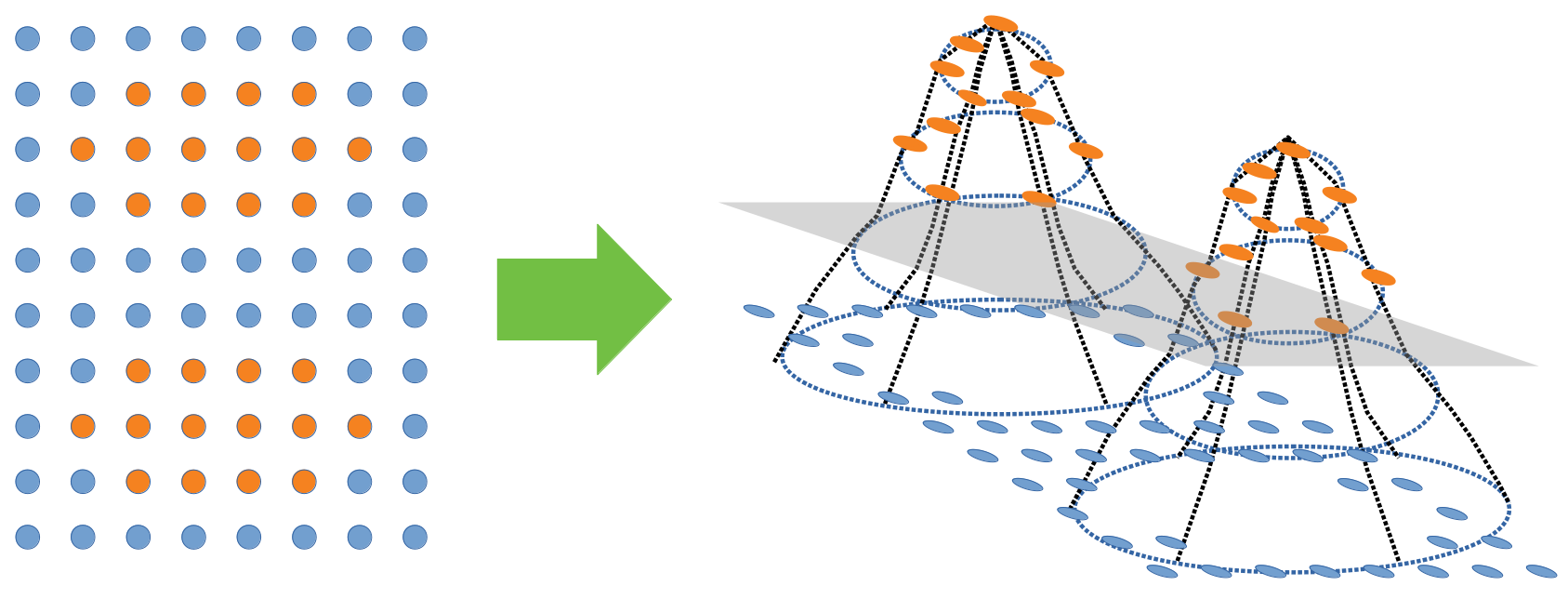
Figure 1: Illustrating data (left) and its feature space mapping using a higher-dimensional kernel (right).

II.1 Kernel Methods

Kernel methods extend linear algorithms to handle nonlinear problems by mapping the input data into a high-dimensional feature space using a nonlinear transformation. However, instead of explicitly performing this transformation, kernel methods rely on computing inner products in the feature space directly using a kernel function [13]. Consider a non-linear map $\phi:\mathbb{R}^{d}\rightarrow\mathcal{F}$, which transforms the input features into a vector space $\mathcal{F}$ known as the feature space. The linear model of a non-linear function $f(\mathbf{x})$ in the feature space is

$$f(\mathbf{x}_{i})=\mathbf{w}_{\phi}^{\top}\phi(\mathbf{x}_{i}),$$ (6)

where $\mathbf{w}_{\phi}$ is the weight vector in the feature space. The cost function becomes

$$J(\mathbf{w}_{\phi})=\frac{1}{N}\sum_{i=1}^{N}\left(y_{i}-\mathbf{w}_{\phi}^{\top}\phi(\mathbf{x}_{i})\right)^{2}.$$ (7)

Solving for $\mathbf{w}_{\phi}$ directly is often computationally expensive due to the high dimensionality of $\mathcal{F}$. Instead, we leverage the representer theorem [14], which states that the optimal solution $\mathbf{w}_{\phi}$ can be expressed as a linear combination of the transformed training samples

$$\mathbf{w}_{\phi}=\sum_{i=1}^{N}\alpha_{i}\phi(\mathbf{x}_{i}).$$ (8)

Substituting into the model, we have

$$f(\mathbf{x})=\sum_{i=1}^{N}\alpha_{i}\phi(\mathbf{x}_{i})^{\top}\phi(\mathbf{x})=\sum_{i=1}^{N}\alpha_{i}k(\mathbf{x}_{i},\mathbf{x}),$$ (9)

where $k(\mathbf{x}_{i},\mathbf{x}_{j})=\phi(\mathbf{x}_{i})^{\top}\phi(\mathbf{x}_{j})$ is the kernel function. For clarity, let us consider kernel regression without regularization. The cost function simplifies to

$$J(\boldsymbol{\alpha})=\frac{1}{N}\sum_{i=1}^{N}\left[y_{i}-\sum_{j=1}^{N}\alpha_{j}k(\mathbf{x}_{j},\mathbf{x}_{i})\right]^{2}=\frac{1}{N}\left\|\mathbf{y}-\mathbf{K}\boldsymbol{\alpha}\right\|^{2},$$ (10)

where $K_{ij}=(\mathbf{x}_{i},\mathbf{x}_{j})$ are elements of the kernel matrix $\mathbf{K}$. Our objective is to find the coefficients $\boldsymbol{\alpha}=[\alpha_{1},\alpha_{2},\dots,\alpha_{N}]^{\top}$ that minimize $J(\boldsymbol{\alpha})$. Minimizing $J(\boldsymbol{\alpha})$ with respect to $\boldsymbol{\alpha}$ leads to the normal equations

$$\boldsymbol{\alpha}=\mathbf{K}^{-1}\mathbf{y}.$$ (11)

Once we have $\boldsymbol{\alpha}$, we can make prediction for any new input $\mathbf{x}$ using Eq. 9. Thus, by using kernel functions, we can work in very high-dimensional (even infinite-dimensional) feature spaces without explicitly computing the mapping $\phi(\mathbf{x})$. Common kernel functions include:

• Linear kernel: $k(\mathbf{x}_{i},\mathbf{x}_{j})=\mathbf{x}_{i}^{\top}\mathbf{x}_{j}$.

• Polynomial kernel: $k(\mathbf{x}_{i},\mathbf{x}_{j})=(\mathbf{x}_{i}^{\top}\mathbf{x}_{j}+c)^{d}$, where $c$ is a constant and $d$ is the degree.

• Gaussian kernel: $k(\mathbf{x}_{i},\mathbf{x}_{j})=\exp\left(-\frac{\|\mathbf{x}_{i}-\mathbf{x}_{j}\|^{2}}{2\sigma^{2}}\right)$.

These kernels allow us to capture complex, nonlinear relationships in the data using algorithms designed for linear models [2].

(c)

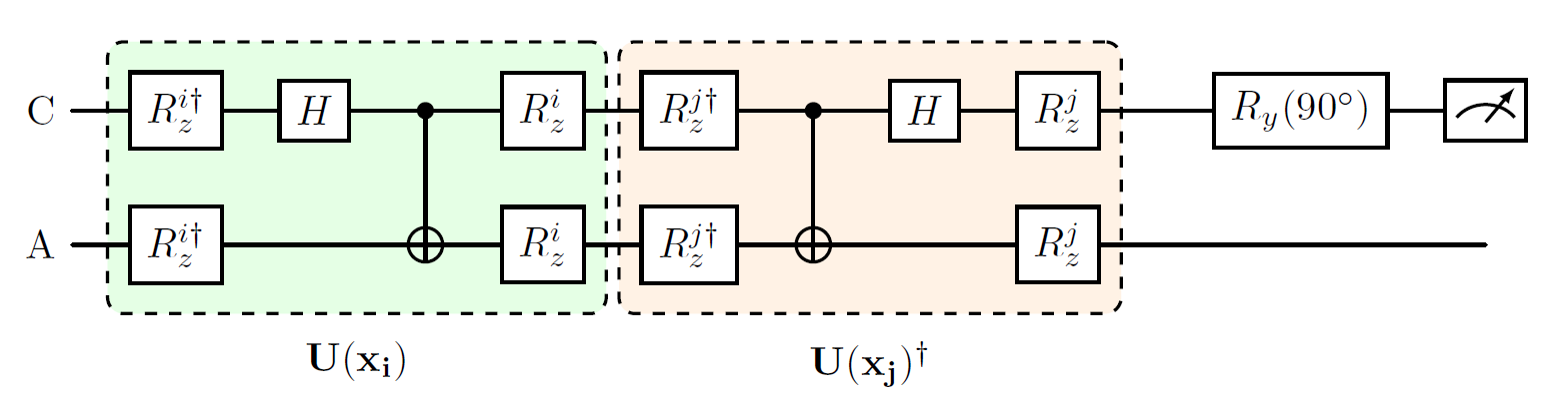
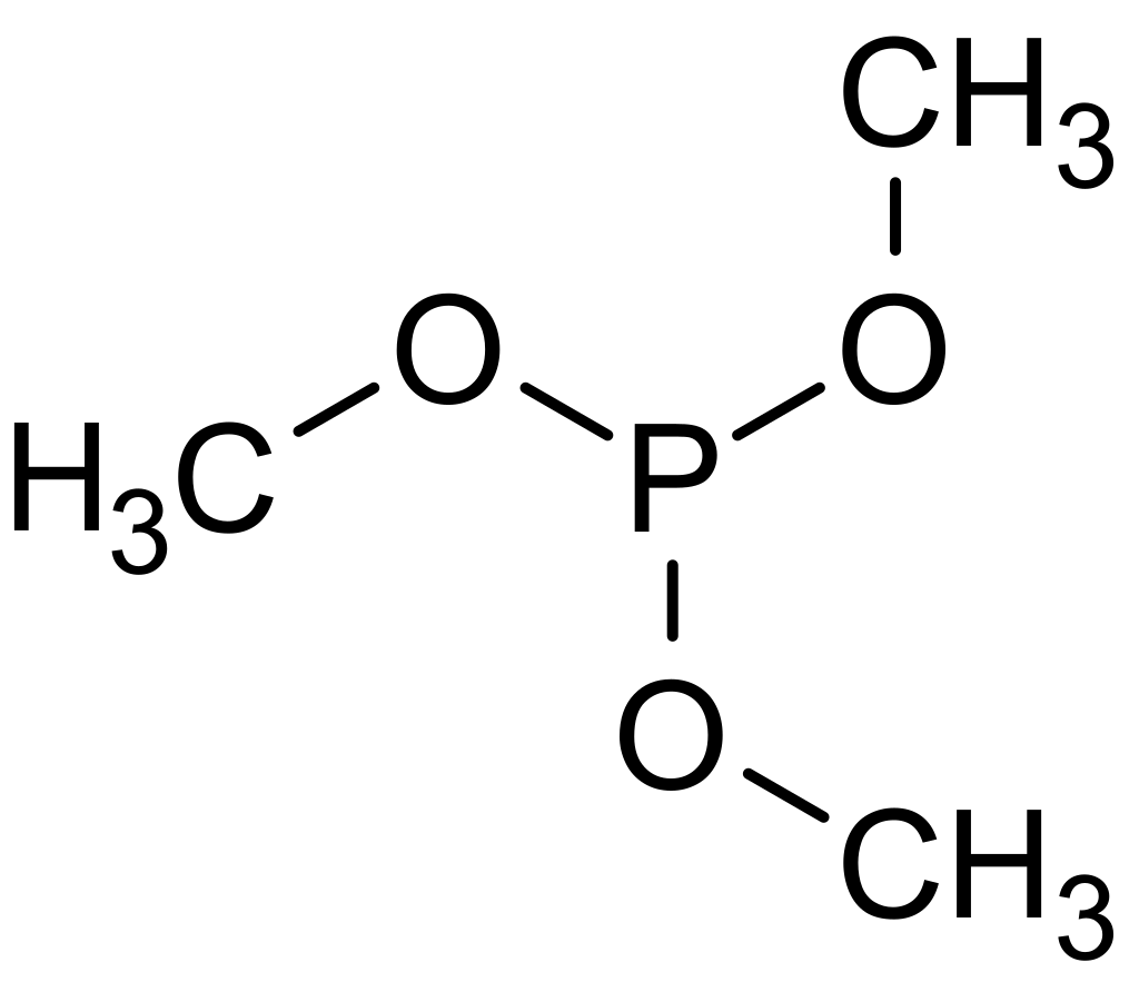
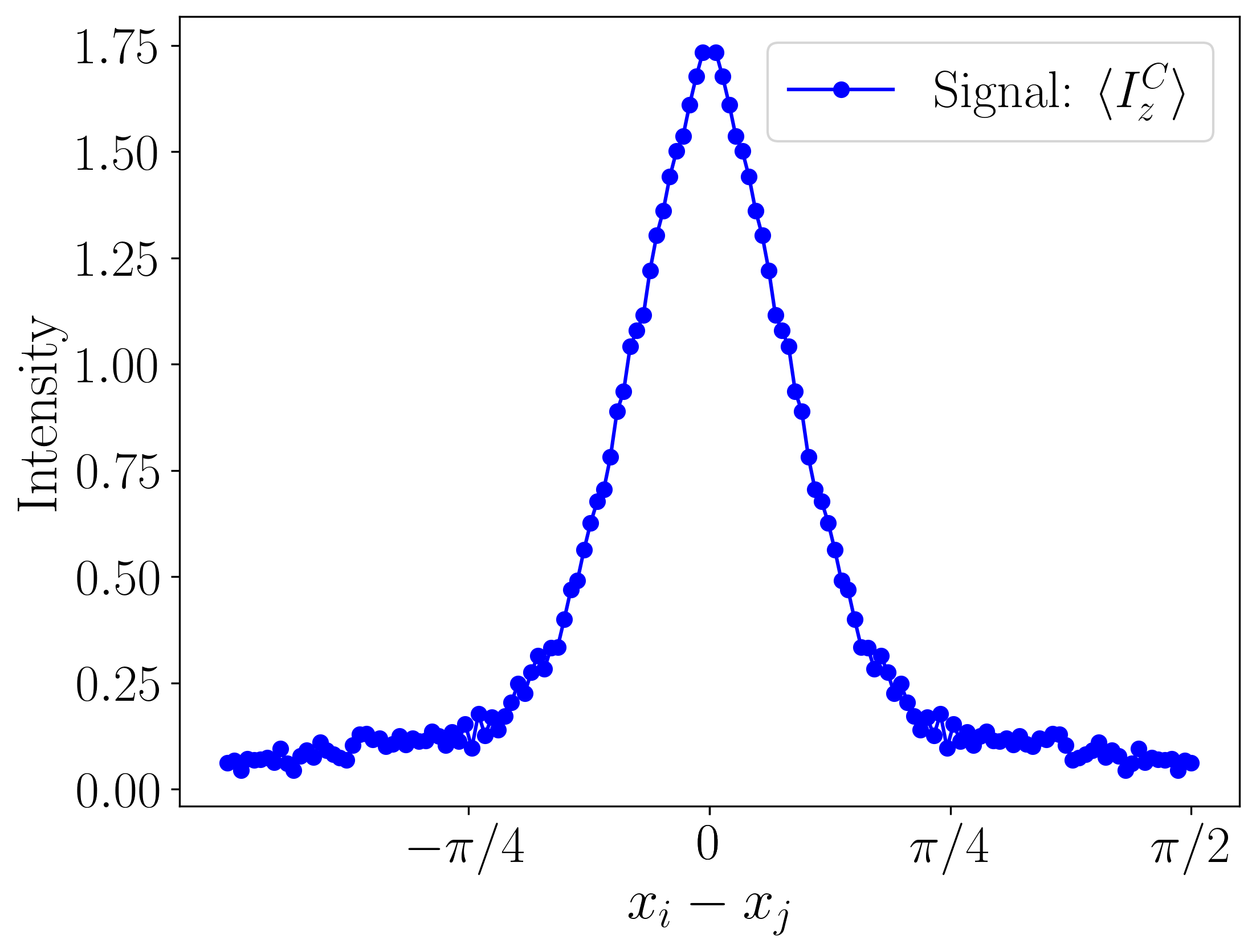
(a) (b) (d)

Figure 2: (a) Geometry of the star-topology register. (b) Molecular structure of trimethyl phosphite, where ³¹P and ¹H spins form central (C) and (A) ancillary qubits. Here $J_{AC}=11.0$ Hz. (c) Quantum circuit for encoding classical inputs $x_{i}$ and $x_{j}$ in terms of unitaries $U(x_{i})$ and $U(x_{j})$, followed by measurement of $z$ magnetization of C qubit. Here, helix represents the dephasing operations on $x$ and $y$ magnetizations C-qubit. (d) Experimentally obtained kernel function for one-dimensional inputs using the quantum kernel in Eq. 18. Assuming the symmetry of the kernel function, the left half is obtained by mirroring the experimentally extracted right half.

II.2 Quantum Kernel Methods

Quantum kernel methods extend classical kernel techniques by utilizing quantum registers to compute kernel functions, capturing complex patterns in data that may be intractable classically. The principal idea is to map the input data into the operator space of the quantum system that exploits the rich algebraic structure of quantum operators, without necessitating a full-scale quantum computer [15]. In our work, we employ nuclear spin qubits in an NMR setup to experimentally extract the quantum kernel.

The quantum feature mapping involves encoding input data points $\mathbf{x}_{i}$ into quantum operators $A(\mathbf{x}_{i})$. We achieve the encoding by associating each data point with a specific unitary transformation $U(\mathbf{x}_{i})$ acting on the quantum system

$$A(\mathbf{x}_{i})=U(\mathbf{x}_{i})A_{0}U^{\dagger}(\mathbf{x}_{i}),$$ (12)

where $A_{0}$ is a reference operator in the system. Here $U(\mathbf{x}_{i})$ are designed such that they efficiently explore the operator space. The quantum kernel is then computed using the Frobenius inner product between operators

$$k(\mathbf{x}_{i},\mathbf{x}_{j})=\text{Tr}\left[A(\mathbf{x}_{i})A(\mathbf{x}_{j})\right].$$ (13)

This kernel function measures the similarity between data points in the operator space, effectively capturing intricate relationships inherent in the data. Detailed methodologies and specific implementations within NMR framework are discussed in the next section.

III Extracting quantum kernels and implementing ML tasks

III.1 Quantum Kernel for Classical Data

Here we use the star system, namely trimethyl phosphite, whose geometry and molecular structure are shown in Fig. 2 (a,b). Here ³¹P and ¹H spins form central (C) and (A) ancillary qubits of the star-topology register. Given a classical input $\mathbf{x}_{i}$, we design the corresponding unitary $U(\mathbf{x}_{i})$ and implment quantum feature map

$$A(\mathbf{x}_{i})=U(\mathbf{x}_{i})I_{z}^{C}U^{\dagger}(\mathbf{x}_{i}),$$ (14)

where $I_{z}^{C}$ is the $z$ component of the spin angular momentum operator of C-qubit. Starting from thermal equilibrium, we destroy the A spin magnetizations with the help of pulsed-field gradients and retain the central spin state in

$$\rho_{eq}^{C}=\frac{1}{2}(1+\epsilon I_{z}^{C}),$$ (15)

where $\epsilon$ is the central spin purity factor. Using Eqs. 13 and 14, the NMR kernel can be written as

$$k_{\text{NMR}}(\mathbf{x}_{i},\mathbf{x}_{j})\propto\text{Tr}(U^{\dagger}(\mathbf{x}_{j})U(\mathbf{x}_{i})\rho_{eq}^{C}U^{\dagger}(\mathbf{x}_{i})U(\mathbf{x}_{j})I_{z}^{C}),$$ (16)

which can be interpreted as the $z$-magnetization of C spin measured after applying, on $\rho_{eq}^{C}$, the unitary $U(\mathbf{x}_{i})$ followed by $U^{\dagger}(\mathbf{x}_{j})$. Assuming the input vectors are one-dimensional, the encoding unitary transformation used for input data is given by

$$U(x_{i})=e^{-ix_{i}I_{z}^{A}}U_{e}e^{ix_{i}I_{z}^{A}},$$ (17)

where $U_{e}$ is the entangling unitary that generates multiple quantum coherences in the system. This idea is motivated by previous work on quantum kernels realized in a solid-state system by Kusumoto et al. [7].

The complete quantum circuit for the process is depicted in Fig. 2 (c). Here, the local gates of the circuit are realized using RF pulses, while the CNOT gates are realized with the help of indirect spin-spin coupling $J_{PH}$. Noting that the Z rotations only add a phase to the $\rho_{eq}^{C}$ and $I_{z}^{C}$ operators, the one-dimensional kernel can be written as

$$k_{\text{NMR}}(x_{i},x_{j})\propto$$

$$\text{Tr}(U_{e}^{\dagger}e^{-i(x_{i}-x_{j})I_{z}^{A}}U_{e}\rho_{eq}^{C}U_{e}^{\dagger}e^{i(x_{i}-x_{j})I_{z}^{A}}U_{e}I_{z}^{C}).$$ (18)

Clearly, $k_{\text{NMR}}(x_{i},x_{j})$ is a function of the difference between the input data points $x_{i}$ and $x_{j}$. The experimental kernel obtained for the one-dimensional inputs is shown in Fig. 2 (d), which is used for the machine learning tasks described in the following.

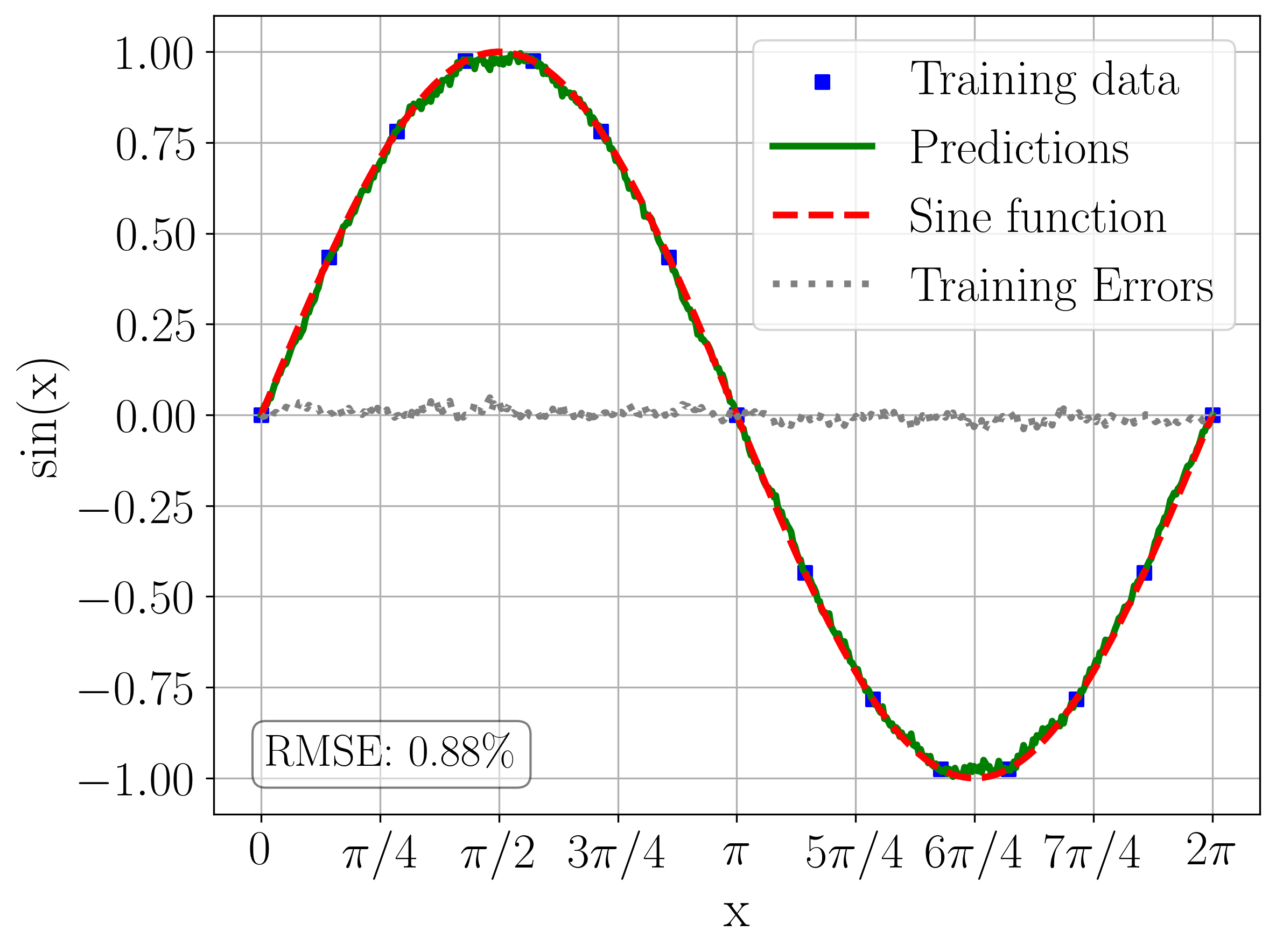
(a)

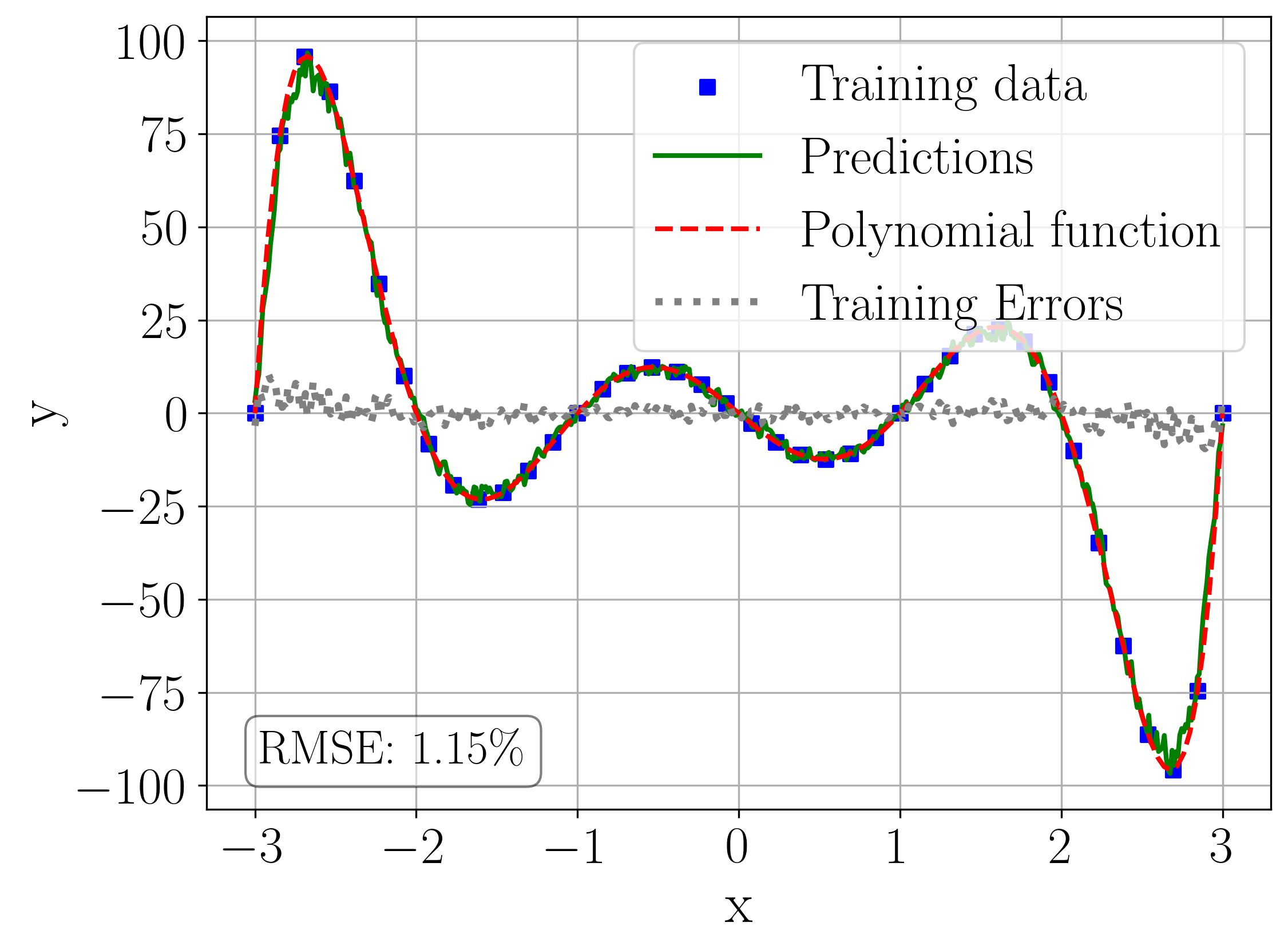
(b)

Figure 3: Regression of (a) sine function with 15 training data points and (b) a seventh-degree polynomial function with 40 training data points.

III.1.1 One-dimensional regression task

Using the experimentally obtained kernel, we can now perform a one-dimensional regression task via the kernel ridge regression method. We choose two examples. In the first example, we choose the target function as a sine curve over one period with a regularly placed training dataset of size 15. Fig. 3 (a) shows the successful regression with an RMS error 0.88%. In the second example, we choose a seventh-degree polynomial $y=(x-3)(x-2)(x-1)x(x+1)(x+2)(x+3)$ with a training dataset of size 40. Fig. 3 (b) shows again a successful regression with an RMS error of 1.15%.

III.1.2 Two-dimensional classification task

Suppose the input data points are $n$-dimensional, i.e., $\mathbf{x_{i}}\in\mathbb{R}^{n}$ such that $\mathbf{x_{i}}=(x_{i}^{(1)},x_{i}^{(2)},\dots,x_{i}^{(n)})$. The data dependent unitary for each input data point of $n$ dimensions is constructed as

$$U(\mathbf{x_{i}}) =\prod_{j=1}^{n}V(x_{i}^{(j)})=\prod_{j=1}^{n}e^{-ix_{i}^{(j)}I_{z}}U_{e}e^{ix_{i}^{(j)}I_{z}},$$ (19)

where we identify $V(x_{i}^{(j)})$ as the encoding unitary for the $j$-th dimension of the input data point $\mathbf{x_{i}}$. Using the above encoding scheme, we now extract the two-dimensional kernel function using Eq. 16 and accordingly a generalization of the circuit shown in Fig. 2 (c). Since this kernel satisfies the symmetry [7]

$$k(\{x_{i}^{(1)},x_{i}^{(2)}\},\{x_{j}^{(1)},x_{j}^{(2)}\})=$$

$$k(\{x_{i}^{(1)}-x_{j}^{(2)},x_{i}^{(2)}-x_{j}^{(2)}\},\{x_{i}^{(1)}-x_{i}^{(2)},0\}),$$ (20)

we can set $x_{j}^{(2)}=0$, and extract the kernel for two-dimensional inputs with only three independent parameters, $x_{i}^{(1)}$, $x_{i}^{(2)}$ and $x_{j}^{(1)}$. Fig. 4 (a) shows the $x_{j}^{(1)}$ slices of the experimental kernel.

(a)

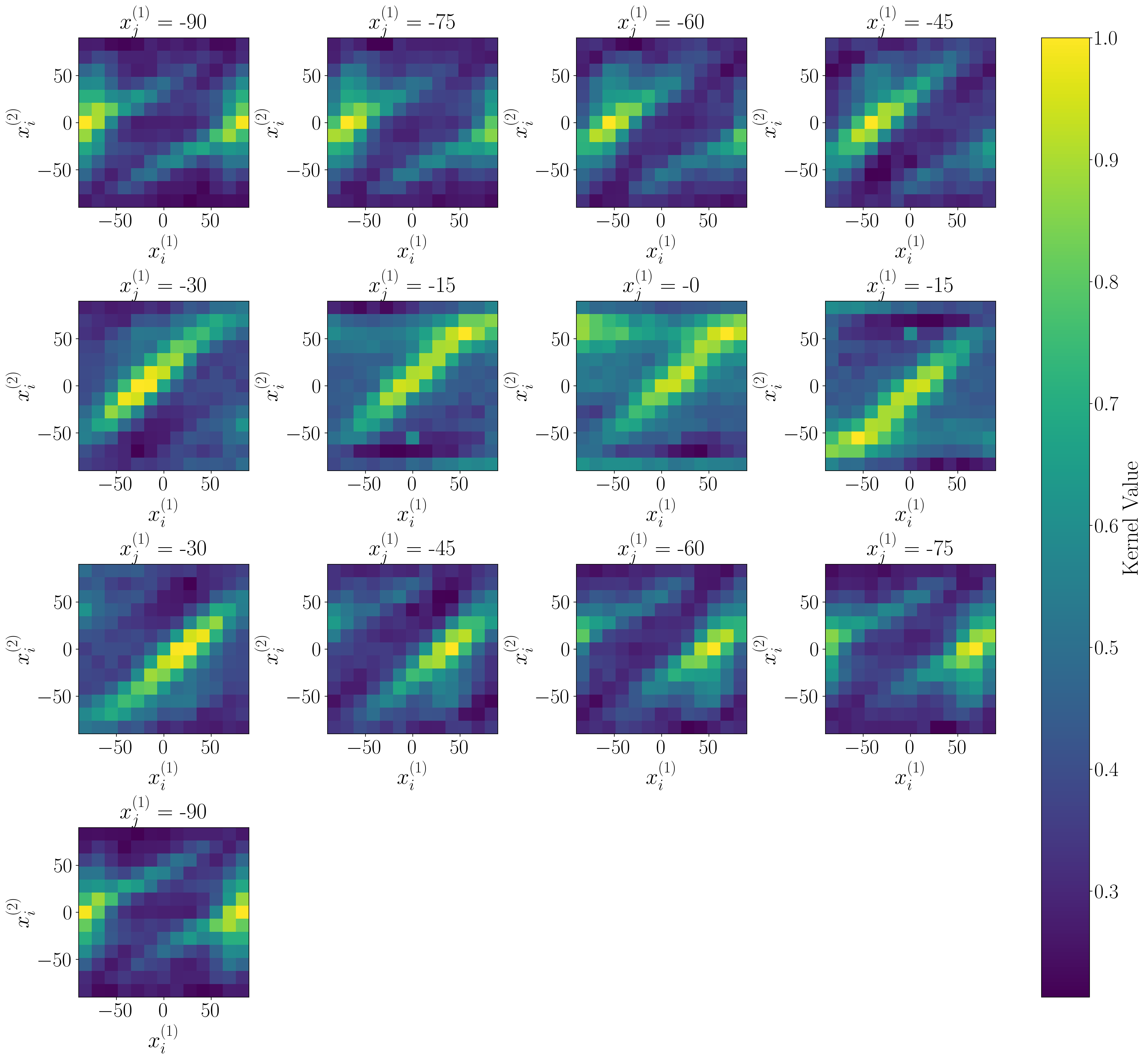
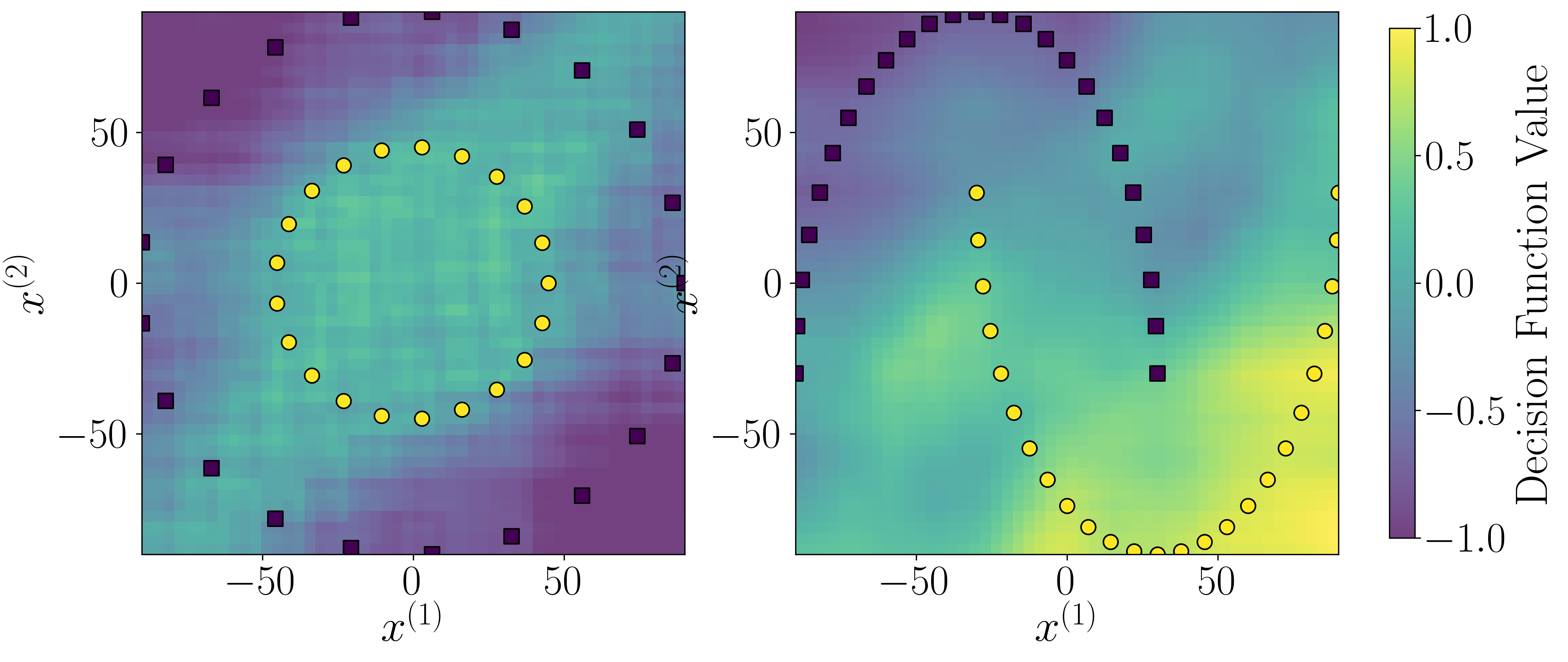
(b) (c)

Figure 4: (a) The $x_{j}^{(1)}$ slices of the experimentally obtained kernel for two-dimensional input. (b,c) Two-dimensional classifications for (b) circles dataset and (c) moons dataset. In both classifications, the squares and circles represent the training data points belonging to two different classes. The background represents the decision function obtained after training.

Using the above experimental kernel, we performed two-dimensional classification tasks using a support vector machine (SVM) classifier. Again we take two different examples of classification, a circular dataset (Fig. 4 (b)) and a moons dataset (4 (c)). In Figs. 4 (b,c), circles and squares show two classes of training datasets. The decision functions learned by the SVM are shown by the backgrounds of Figs. 4 (b,c). The hinge loss values, that quantify errors in these classifications, are 0.15 and 0.08 respectively. These results show that the choice of the protocol to compute the kernel is fairly reliable and has the potential to carry out standard ML tasks. In the following, we explore the possibility of extending the kernel method to quantum inputs, which enables us to perform specific quantum tasks.

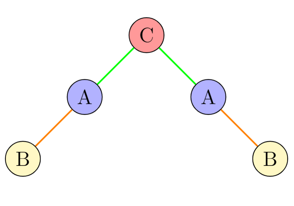
(a)

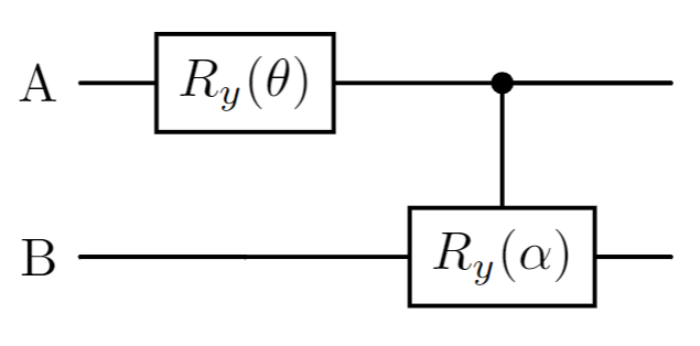
(b)

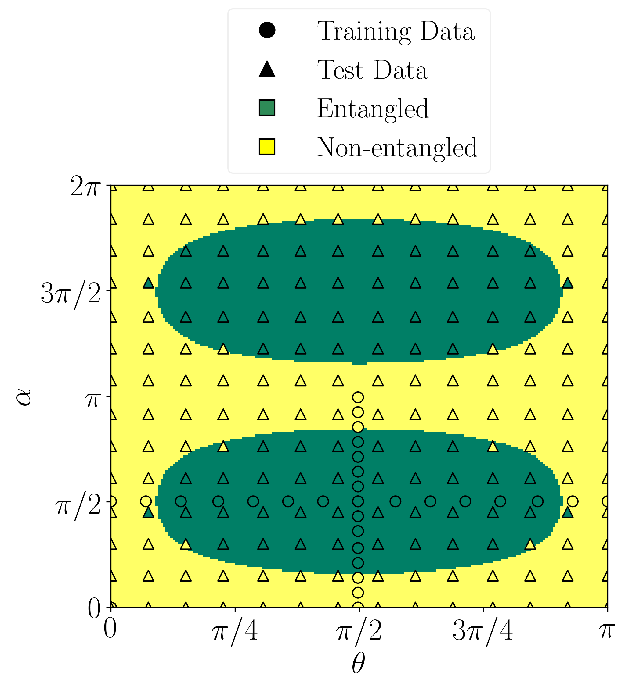
(c)

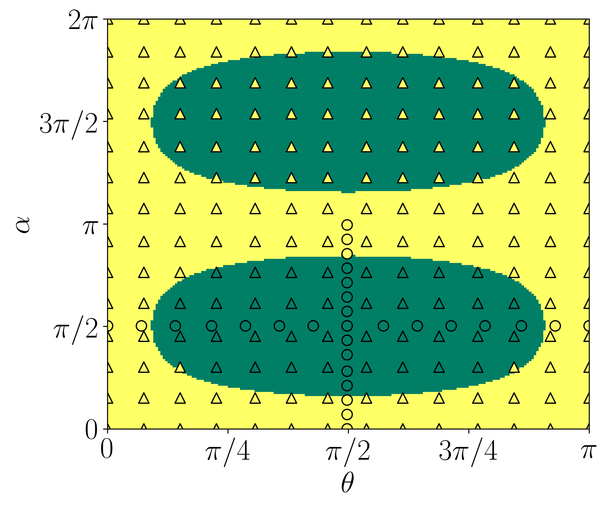
(d)

Figure 5: (a) The geometry of the spin register used for the entanglement classification task. (b) Quantum circuit for encoding unitaries $U_{i}$ parametrized by $\theta$ and $\alpha$. (c) The background indicates the actual classification of entangling (inside elliptical patches) and nonentangling (outside elliptical patches) when acted on the thermal equilibrium state $\rho_{0}$ in Eq. 22. The circles represent 30 training unitary operators, and the triangles are the test unitary operators. (d) Same as (c), except with a classical Gaussian kernel trained on the parameter space $(\theta,\alpha)$. Note that the quantum kernel in (c) recognizes the upper entangling zone even without a single training point there, while the classical kernel in (d) completely fails to recognize the upper entangling zone.

III.2 Quantum Kernel for Quantum Data

As an example for a quantum ML task, we take up the task of determining whether a given unitary transformation $U$ entangles any given initial mixed state $\rho$. The entanglement classification task is a binary classification problem where the input data is a unitary transformation and the output is a binary label indicating whether the transformation is entangling or not for a particular initial mixed state. It is a nontrivial problem, which is discussed by Serrano-Ensástiga and Martin [16].

We now approach the above problem using the quantum kernel method by taking a set of unitary transformation $U$ as the quantum input data. The quantum kernel method offers significant advantages over classical kernels. Firstly, unitary transformations do not require parameterization (except for training), as they can be fed directly into the kernel model. Secondly, the quantum kernels with quantum inputs have the ability to predict the labels of inputs that are categorically different from the training inputs [17]. To handle a quantum input, we propose a quantum kernel

$$k(U_{i},U_{j})=\text{Tr}(A(U_{i})A(U_{j})),$$ (21)

where $A(U_{i})=V(U_{i})A_{0}V^{\dagger}(U_{i})$ is the quantum feature map for the unitary $U_{i}$ with the encoding unitary $V(U_{i})=U_{i}U_{e}U_{i}^{\dagger}$ and $A_{0}$ is a suitable reference operator in the system. The kernel function $k(U_{i},U_{j})$ measures the similarity between the unitaries $U_{i}$ and $U_{j}$ in the operator space. We now assume a quantum register of geometry shown in Fig. 5 (a). The central qubit C is connected to A qubits, and each A qubit is connected to a B qubit. The input unitaries $U_{i}$ act on A and B qubits as shown in Fig. 5 (b), and then $U_{e}$ entangles A qubits with C qubit. The quantum kernel for the entanglement classification task is computed using Eq. 16 with the new encoding scheme described above. The numerical results of the entanglement classification task are shown in Fig. 5 (c,d).

We classify the unitary operators acting on the thermal equilibrium state

$$\rho_{0}=e^{-\beta H_{Z}}/4$$ (22)

of a two spin-$\frac{1}{2}$ particles subject to Hamiltonian $H_{Z}=-0.5\cdot(\sigma_{z}^{(1)}+\sigma_{z}^{(2)})$ and maintained at an inverse temperature $\beta=1.5$. The numerical results of the classification are shown in Fig. 5 (c). Here, the background shades represent the actual entanglement labels of the operators, which are obtained by using the logarithmic negativity as the entanglement witness for the final states [18]. Here training is done with 30 operators, chosen from only the lower part of the parameter space as indicated by circles. The kernel model is then tested on 196 operators uniformly distributed over the entire parameter space. The model is found to classify the operators with an accuracy of 94%. Interestingly, we observe an extrapolation ability of the proposed kernel model beyond the training area. This is because a kernel with quantum inputs measures the similarity of the inputs directly in the quantum operator space and not in the classical parameter space [19]. We now replace the quantum kernel with a classical Gaussian kernel that takes in parameters $(\theta,\alpha)$ as inputs [20]. The classification results with the classical kernel with the same training points (as in the quantum case) are shown in Fig. 5 (d). Note that, while the classical kernel is able to recognize the lower entangling area where training points are located, it completely fails to recognize the upper entangling area. This example illustrates the power of quantum kernels over classical kernels, especially for quantum tasks.

Additionally, as mentioned before, unlike classical kernels, the quantum kernel can also handle nonparameterized unitaries. We tested the above quantum kernel (trained on the same set as above) with 100 nonparameterized random unitary operators. We found it to correctly classify up to 84% of the random unitary operators, once again confirming its ability to handle quantum data directly.

IV Conclusions

Quantum kernels offer a practical approach for exploring the high-dimensional feature spaces inherent in quantum systems. In this work, we have demonstrated the implementation of quantum kernel methods using NMR-based spin registers. By leveraging the symmetries of a 10-qubit star-topology NMR system, we encoded classical data into multiple-quantum coherence orders through data-dependent unitary transforms and computed the kernel function through experimental measurements. Our results show that the quantum kernel method can effectively perform classical machine learning tasks such as one-dimensional regression and two-dimensional classification.. Furthermore, by extending the register to a double-layered star configuration, we introduced a quantum kernel capable of handling non-parametrized unitary operator inputs, which can then perform quantum classification tasks. We illustrated the power of quantum kernel by successfully classifying unitary operators depending on whether they generate entanglement or not when acted on a thermal state. When a large set of high-dimensional unitaries needs to be classified, the standard method of tomography is no longer feasible. In such a scenario, a well-trained quantum kernel can be far more efficient in classification. This work opens new possibilities for processing quantum data directly, marking a step toward realizing fully quantum machine learning systems. Our findings underscore the potential of quantum kernels in advancing quantum machine learning, providing a promising avenue for future research in more complex quantum tasks and larger-scale implementations. Future work will focus on the experimental realization of the entanglement classification task and extending these methods to more complex quantum challenges.

V Acknowledgements

Authors gratefully acknowledge discussions with Arijit Chatterjee, Vishal Varma, and Keshav V. ChatGPT was helpful in generating simulation codes for this study. T.S.M. acknowledges funding from DST/ICPS/QuST/2019/Q67 and I-HUB QTF.

References

- [1] Bernhard Schölkopf and Alexander J. Smola. Learning with Kernels: Support Vector Machines, Regularization, Optimization, and Beyond. MIT Press, 2002.
- [2] John Shawe-Taylor and Nello Cristianini. Kernel Methods for Pattern Analysis. Cambridge University Press, 2004.
- [3] Aram W. Harrow, Avinatan Hassidim, and Seth Lloyd. Quantum algorithm for linear systems of equations. Phys. Rev. Lett., 103:150502, Oct 2009.
- [4] Maria Schuld and Nathan Killoran. Quantum machine learning in feature hilbert spaces. Physical Review Letters, 122:040504, 2018.
- [5] Maria Schuld and Nathan Killoran. Quantum machine learning in feature hilbert spaces. Phys. Rev. Lett., 122:040504, Feb 2019.
- [6] Maria Schuld. Supervised quantum machine learning models are kernel methods. Quantum, 5:531, 2021.
- [7] Takeru Kusumoto et al. Experimental quantum kernel trick with nuclear spins in a solid. npj Quantum Information, 5:39, 2019.
- [8] Karol Bartkiewicz et al. Experimental kernel-based quantum machine learning in finite feature space. Scientific Reports, 9:63, 2019.
- [9] E. Peters et al. Machine learning of high dimensional data on a noisy quantum processor. npj Quantum Information, 7:86, 2021.
- [10] T. S. Mahesh, Deepak Khurana, Krithika V R, Sreejith G J, and Sudheer Kumar. Star-topology registers: Nmr and quantum information perspectives. Journal of Physics: Condensed Matter, 33, 2021.
- [11] George A. F. Seber and Alan J. Lee. Linear Regression Analysis. Wiley, 2 edition, 2012.
- [12] Douglas C. Montgomery, Elizabeth A. Peck, and Geoffrey G. Vining. Introduction to Linear Regression Analysis. Wiley, 5 edition, 2012.
- [13] Thomas Hofmann, Bernhard Schölkopf, and Alexander J. Smola. Kernel methods in machine learning. The Annals of Statistics, 36(3):1171–1220, 2008.
- [14] Bernhard Schölkopf, Ralf Herbrich, and Alex J. Smola. A generalized representer theorem. In David Helmbold and Bob Williamson, editors, Computational Learning Theory: 14th Annual Conference on Computational Learning Theory, COLT 2001 and 5th European Conference on Computational Learning Theory, EuroCOLT 2001, volume 2111 of Lecture Notes in Computer Science, pages 416–426, Berlin, Germany, 2001. Springer.
- [15] Maria Schuld. Quantum models as kernel methods. In Machine Learning with Quantum Computers, pages 125–144. Springer, Cham, 2021.
- [16] Eduardo Serrano-Ensástiga and John Martin. Maximum entanglement of mixed symmetric states under unitary transformations. SciPost Physics, 15:120, 2023.
- [17] Yanqi Song, Jing Li, Yusen Wu, Sujuan Qin, Qiaoyan Wen, and Fei Gao. Quantum phase recognition via quantum kernel methods. Quantum, 7:981, 2021.
- [18] M. B. Plenio. Logarithmic negativity: A full entanglement monotone that is not convex. Physical Review Letters, 95(9):090503, 2005.
- [19] Vanio Markov, Vladimir Rastunkov, and Daniel Fry. Quantum time series similarity measures and quantum temporal kernels, 2024.
- [20] F. Pedregosa, G. Varoquaux, A. Gramfort, V. Michel, B. Thirion, O. Grisel, M. Blondel, P. Prettenhofer, R. Weiss, V. Dubourg, J. Vanderplas, A. Passos, D. Cournapeau, M. Brucher, M. Perrot, and E. Duchesnay. scikit-learn: Machine Learning in Python - Gaussian Process. Scikit-learn Developers, 2024. Available at https://scikit-learn.org/stable/modules/gaussian_process.html.