Enhancing Convergence of Decentralized Gradient Tracking
under the KL Property

Abstract

We study decentralized multiagent optimization over networks, modeled as undirected graphs. The optimization problem consists of minimizing a nonconvex smooth function plus a convex extended-value function, which enforces constraints or extra structure on the solution (e.g., sparsity, low-rank). We further assume that the objective function satisfies the Kurdyka-Łojasiewicz (KL) property, with given exponent $\theta\in[0,1)$. The KL property is satisfied by several (nonconvex) functions of practical interest, e.g., arising from machine learning applications; in the centralized setting, it permits to achieve strong convergence guarantees. Here we establish convergence of the same type for the notorious decentralized gradient-tracking-based algorithm SONATA, first proposed in[43]. Specifically, (i) when $\theta\in(0,1/2]$, the sequence generated by SONATA converges to a stationary solution of the problem at R-linear rate; (ii) when $\theta\in(1/2,1)$, sublinear rate is certified; and finally (iii) when $\theta=0$, the iterates will either converge in a finite number of steps or converges at R-linear rate. This matches the convergence behavior of centralized proximal-gradient algorithms except when $\theta=0$. Numerical results validate our theoretical findings.

Key words. distributed optimization, decentralized methods, nonconvex optimization, gradient-tracking, Kurdyka-Łojasiewicz, linear rate.

1 Introduction

This paper studies nonconvex, nonsmooth optimization problem over networks of the following form:

$$\begin{array}[]{rl}\underset{{x}\in\mathbb{R}^{d}}{\min}&u({x}):=f({x})+r({x}),\end{array}$$ (P)

where

$$f({x}):={\frac{1}{m}}\sum^{{m}}_{i=1}{f_{i}({x})},$$ (1)

with each $f_{i}:\mathbb{R}^{d}\to\mathbb{R}$  being the cost function of agent $i=1,\ldots,m$, assumed to be $L_{i}$-smooth (possibly nonconvex) and known only to agent $i$; $r:\mathbb{R}^{d}\to\mathbb{R}\cup\{-\infty,+\infty\}$  is a nonsmooth convex (extended-value) function, known to all agents, which can be used to enforce shared constraints or specific structures on the solution (e.g., sparsity). Agents are connected through a communication network, modeled as a fixed, undirected graph.

Problem (P) has a wide range of applications, such as network information processing, telecommunications and multi-agent control. Here, we are particularly interested in machine learning problems, specifically supervised learning. Examples include logistic regression, SVM, LASSO and deep learning. Each $f_{i}$ represents the empirical risk measuring the mismatch between the model (parameterized by ${x}$) to be learnt and the dataset owned by agent $i$; and $r$ plays the role of the regularizer. A vast range of these problems possess some structural properties, notably in the form of some growth property, which can be leveraged to enhance convergence of decentralized solution methods. In this paper we target the so-called Kurdyka-Łojasiewicz (KL) property, due to its vast range of applicability. The class of functions satisfying the KL property is ubiquitous, ranging from applications in optimization [31, 3, 4, 5, 12, 17, 27], machine learning (logistic regression, LASSO, and the Principal Component Analysis (PCA) are notorious examples), deep neural network [24], dynamical systems, and partial differential equations; see [11] and the references therein.

The KL property was first introduced by Łojasiewicz [32] for real analytic functions, then Kurdyka extended it to functions defined on a generalization of semialgebraic and subanalytic geometry called the o-minimal structure [23]. More recently, it was extended to nonsmooth subanalytic functions by Bolte et al. [10]. In its simplest form [4], we say that a $C^{1}$ function $f:\mathbb{R}^{d}\to\mathbb{R}$ satisfies the KL property with exponent $\theta\in[0,1)$ at $\bar{x}\in\mathbb{R}^{d}$ (possibly critical) if there exists $\theta\in[0,1)$ and some problem-dependent $c>0$ such that

$$||\nabla f(x)||\,\geq c\,|f(x)-f(\bar{x})|^{\theta}.$$ (2)

Ensuring a lower bound on the gradient magnitude in the proximity of $\bar{x}$, this condition stipulates that the function $f$ cannot be arbitrarily flat around $\bar{x}$. As for its nonsmooth counterpart, one can refer to Sec. 2.1 for more details.

In the recent years, the KL property has been successfully leveraged to enhance convergence of several solution methods for nonconvex, nonsmooth, centralized optimization problems; examples include inexact first-order methods [5], alternating (proximal) minimization algorithms [4], and parallel methods [13]. In particular, under the KL, the entire sequence generated by these algorithms is proved to converge to a stationary solution (in contrast with the much weaker guarantees in the absence of KL, certifying subsequence convergence). The convergence rate is dictated by the KL exponent $\theta$, namely: when $\theta\in(0,1/2]$, linear rate is certified whereas sublinear convergence is proved when $\theta\in(1/2,1)$; finally, when $\theta=0$, the sequence converges in a finite number of iterations.

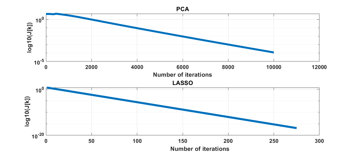
Figure 1: Distance of the iterates ($x_{i}^{\nu}$, $i\in[m]$ ) from a stationary solution ($x^{*}$) of the PCA (upper panel) and LASSO (lower panel) problems, defined as $\mathcal{P}^{\nu}:=\sqrt{\sum_{i=1}^{m}\|x_{i}^{\nu}-x^{*}\|^{2}}$, versus the iterations $\nu$.

This leads to the natural question whether these strong convergence guarantees can be inherited by decentralized algorithms. To the best of our knowledge, the existing literature on distributed algorithms does not provide a satisfactory answer (see Sec. 1.2 for a detailed review of the state of the art). Here we only point out that none of the existing analyses of decentralized algorithms [40, 46, 15, 43, 41] applicable to problem (P) exploit the KL property of $u$. As a consequence, if nevertheless invoked, they would predict much more pessimistic convergence rates than what is certified in the centralized setting. For instance, when applied to (P) under the KL with $\theta\in(0,1/2]$, they would claim sublinear convergence of some surrogate distance from stationarity, which contrasts the much more favorable linear convergence of the entire sequence established for a variety of centralized first-order methods applied to (P). These pessimistic predictions are confuted by experiments. Two examples are reported in Fig. 1, where the the decentralized algorithm SONATA [40] is applied to two nonconvex instances of (P) over a network modeled as an Erdos-Renyi graph–the LASSO problem with SCAD regularizer  [27] (cf. Sec. 2.1) and the PCA problem. The objective functions of both problems satisfy the KL property with exponent $1/2$. The figures plot the distance of the SONATA’s iterates from a stationary solution versus number of iterations, certifying linear convergence of the sequence for both problems. This fact has no theoretical backing.

This paper fills this gap. As a case-study, we focus on the gradient tracking-based decentralized scheme SONATA, firstly proposed in [43]. We provide a full characterization of its convergence rate, for the entire range of the KL exponent $\theta\in[0,1)$, matching convergence results of the proximal gradient algorithm in the centralized setting.

1.1 Main contributions

Our technical contributions can be summarized as follow.

$\bullet$ Convergence rate under the KL of $u$: We establish convergence of the sequence generated by SONATA to stationary solutions of (P), and characterize its convergence rate, under different values of the KL exponent of of $u$. More specifically,

• When $\theta\in(0,1/2]$, the sequence generated by SONATA is proved to converge R-linearly. The number of communication rounds to reach an $\epsilon$-stationary solution (under proper tuning) reads

  $$\mathcal{\tilde{O}}\left(\frac{L}{\kappa^{1/\theta}}\frac{1}{1-\rho}\text{log}(1/\epsilon)\right),$$

  where $L:=\frac{1}{m}\sum_{i=1}^{m}L_{i}$, with $L_{i}$ being the smoothness constant of $f_{i}$; $\kappa$ is a parameter related with the KL property of $u$ (see Def. 1), and $\rho$ represents the network connectivity (see (6) for the formal definition). The $\mathcal{\tilde{O}}$ notation hides log-dependencies on $L$, $\kappa$, $\theta$ and $L_{\text{mx}}:=\max_{i\in[m]}L_{i}$.

• For $\theta\in(1/2,1)$, sublinear convergence of the sequence is established, yielding rates for $\epsilon$-stationarity of the order

  $$\mathcal{O}(\epsilon^{-\frac{2\theta-1}{1-\theta}}).$$

• When $\theta=0$, the sequence either convergences to a stationary solution in a finite number of iterations or converges at R-linear rate independent of $\kappa$.

Notably, the rates in (i) and (ii) match those of the centralized proximal gradient algorithm (up to universal constants).

$\bullet$ New convergence analysis: We introduce a new line of analysis that explicitly leverage the KL property, departing from traditional techniques employed to study centralized and decentralized algorithms, as detailed next.

Classical proofs–establishing linear convergence of first-order methods under the KL property (with $\theta=1/2)$ of the objective function–focused primarily on centralized settings [3, 4, 5, 12, 17, 27, 13]. They strongly rely on the objective function’s monotonic decrease along algorithmic trajectories. However, when it comes to decentralized algorithms, this monotonicity is disrupted by disagreements among agents’ iterates, introducing perturbations that impair the descent of the objective function $u$. This issue is addressed in [51, 14] by constructing a Lyapunov function that suitably combines agents’ objectives $f_{i}$’s with consensus errors, and monotonically decreases along the algorithm trajectories, albeit limited to unconstrained, smooth instances of (P). Assuming this Lyapunov function is a KL function with $\theta=1/2$, linear convergence of the decentralized algorithms [51, 14] was proved, mirroring techniques used in centralized settings [3, 4, 12, 17, 27, 5]. Unfortunately, the KL property of the Lyapunov function or its exponent value do not transfer to the objective function $u$ of the optimization problem, and vice versa. This is because the KL property is not closed with respect to the operations used to build the Lyapunov function from the objective function. Consequently, the challenge of establishing convergence guarantees for decentralized algorithms under the KL property of the objective function–comparable to those certified in centralized settings–remains unresolved.

Our novel approach hinges on the KL property of the objective function $u$. First, we establish asymptotic convergence of the objective function gap and consensus and tracking errors, along the iterates produced by the SONATA algorithm, through the monotonically decaying trajectory of a suitably constructed Lyapunov function. This guarantees that, after a sufficiently large but finite number of iterations–such that the function value gap falls below a critical threshold–the KL property of the objective function can be engaged. Consequently convergence of the entire sequence to a critical point of $u$ is established, at enhanced convergence rate.

1.2 Related works

Centralized setting: The KL property has been widely utilized in the convergence analysis of centralized optimization methods. The pioneering study of [1] marks the initial use of the KL property to demonstrate sequence convergence to stationary solutions of a variety of algorithms satisfying certain decent properties. However, no convergence rate analysis was established. The followup works  [3, 4, 12, 17, 27, 5, 13] did provide a convergence rate analysis of these algorithms, specifically: the proximal gradient [3], the alternating proximal minimization algorithm [4], the inexact Gauss–Seidel method [5], the Proximal alternating linearized minimization algorithm [12], the alternating forward-backward splitting method [17], and the (parallel) asynchronous method known as FLEXA [13]. Other studies [7, 34, 36, 37] have expanded the class of KL functions and relaxed algorithmic constraints while maintaining the same strong convergence guarantees. Specifically, [7] extends the KL property to include symmetric and strong KL variations; and [34, 36, 37] modify algorithm requirements by permitting an additive error term in the relative error condition [34] and accommodating a nonmonotone descent flow [36]. Notably, [37] integrates both modifications in their analytical framework.

Decentralized setting: Decentralized algorithms for various instances of Problem (P) have received significat attention in the last few years [21, 9, 16, 47, 44, 19, 40, 45, 53]. Specifically, early studies  [21, 44, 19, 45] consider smooth objectives (i.e., $r=0$) whereas [16, 47, 40, 9, 53] extended to constraints or composite structures, under the assumption of bounded (sub)gradient of the objective loss along the iterates of the algorithm. This restriction has been removed in [53, 40], with [40] providing also a convergence rate analysis (applicable to time-varying networks). None of the aforementioned works exploit any growing property of the objective function, such as the KL, if any. This leads to pessimistic convergence guarantees (asymptotic convergence only or sublinear convergence rates), which contrasts with the results in the centralized setting discussed above and is inconsistent with the numerical results presented in Fig. 1 (Sec. 1) and Sec.5.

Works exploiting explicitly some (postulated) function growth to enhance convergence guarantees of decentralized algorithms applied to special instances of (P), include [30, 49, 50, 46, 51, 14]. Specifically, linear rate of the considered decentralized algorithms is proved under the restricted secant condition [30, 49], the Polyak-Łojasiewicz (PL) condition [50], and the Luo-Tseng error bound condition [46]. However, in the nonconvex setting, all these conditions are more stringent than the KL property (with exponent 1/2) [35]. Furthermore, convergence techniques therein closely mirror those used for strongly convex functions, which are not useful in the setting considered in this paper.

On the other hand, while studies such as [14, 51] have utilized the KL property in the convergence analysis of some decentralized algorithms, they have not conclusively achieved the desired outcomes. As discussed in Sec 1.1 , these works postulate the KL property of specifically constructed Lyapunov functions that meet the necessary conditions for convergence, rather than of the original objective functions. The link between the KL property of the objective function and such Lyapunov functions remains unclear, highlighting a gap in the current literature.

1.3 Notation and paper organization

Throughout the paper, we will use the following notation. For any integer $m$, we write $[m]:=\{1,2,\cdots,m\}$. We user the convention that $0^{0}=0$. We denote by $[c_{1}\leq(<)u\leq(<)c_{2}]:=\{x:c_{1}\leq(<)u(x)\leq(<)c_{2}\}$ the level set of the function $u$ at $c\in\mathbb{R}$. We will use capital letters to represent matrices. In particular, $1$ denotes the vector of all ones (whose dimensions are clear from the context); $J:=11^{\top}/n$ is the projection onto the consensus space. We use $\|\cdot\|_{p}$ to denote the $\ell_{p}$-norm of any input vector ($\|\cdot\|$ will be the Euclidean norm) whereas $\|\cdot\|_{p}$ represents the operator norm induced by the $\ell_{p}$-norm when the input is a matrix (with $\|\cdot\|$ being the Frobenius norm). Several operators appear in the paper. Given a proper, nonconvex function $f$, $\partial f(x)$ denotes the (limiting) subdifferential of $f$ at $x$ [38, Def. 8.3(b)]. Given $x\in\mathbb{R}^{d}$ and $r:\mathbb{R}\rightarrow\mathbb{R}\cup\{-\infty,\infty\}$, $\texttt{prox}_{\alpha r}(x)$ denotes the proximal operator, defined as

$$\texttt{prox}_{\alpha r}(x):=\displaystyle{\text{argmin}}_{y\in\mathbb{R}^{d}}r(y)+\frac{1}{2\alpha}\|x-y\|^{2}.$$

The rest of the paper is organized as following. Sec. 2 introduces the problem formulation along with the underlying assumptions. Sec. 3 presents the asymptotic convergence analysis of SONATA, which is instrumental to engage the KL property to enhance the convergence rate. Sec. 4 contains the main technical result of the paper: the convergence rate analysis of SONATA under the KL property. Finally, some numerical experiments are presented in Sec. 5.

2 Problem Setup and Background

We study the Problem (P) over a communication network. Followings are standard assumptions on (P).

Assumption 1 (objective function).

• Each $f_{i}:\mathbb{R}^{d}\rightarrow\mathbb{R}$ is continuously differentiable, and $\nabla f_{i}$ is $L_{i}-$Lipschitz, with $L_{i}<\infty$;

• $r:\mathbb{R}^{d}\rightarrow\mathbb{R}\cup\{-\infty,\infty\}$ is convex, proper and lower-semicontinuous;

• $u:\mathbb{R}^{d}\rightarrow\mathbb{R}$ is lower bounded by some $\underline{u}\in\mathbb{R}$.

Associated with Assumption 1, we define the following quantities used throughout the paper.

$$L_{\text{mx}}:=\max_{i\in[m]}L_{i},\quad\text{and}\quad L:=\frac{1}{m}\sum_{i=1}^{m}L_{i}.$$ (3)

The communication network of the agents is modeled as a time-invariant undirected graph $\mathcal{G}:=(\mathcal{V},\mathcal{E})$, with the vertex set $\mathcal{V}:=\{1,...,m\}$ and the edge set $\mathcal{E}:=\{(i,j)|i,j\in\cal{V}\}$ representing the set of agents and the communication links, respectively. Specifically, $(i,j)\in\mathcal{E}$ if and only if there exists a communication link between agent $i$ and $j$. We make the blanket assumption that $\mathcal{G}$ is connected.

2.1 The KL property: definitions and illustrative examples

In this section, we formally introduce the KL property for $u$ along with some examples of KL functions arising from several applications.

The general definition of the KL can be found in [5]. Here we focus more specifically on functions that are sharp up to some reparametrization, using the so-called desingularizing function, denoted by $\phi:\mathbb{R}\rightarrow\mathbb{R}$. This function turns a singular region–a region where the gradients are arbitrarily small–into a regular region–where the gradients are bounded away from zero. A widely used desingularizing function is $\phi(s):=cs^{1-\theta}$, for some $\theta\in[0,1)$ and $c>0$, firstly introduced in [32]. More specifically, the KL property equipped with this desingularizing function reads as follows.

Definition 1.

(KL property)[27] A proper closed function $f$ satisfies the KL property at $\bar{x}\in\text{dom}f$ with exponent $\theta\in[0,1)$ if there exists a neighborhood $E$ of $\bar{x}$ and parameters $\kappa,\eta\in(0,\infty)$ such that

$$\|g_{x}\|\geq\kappa(f(x)-f(\bar{x}))^{\theta},$$ (4)

for all $x\in E\cap[f(\bar{x})<f<f(\bar{x})+\eta]$ and $g_{x}\in\partial f(x)$. We call the function $f$ a KL function with exponent $\theta$ if it satisfies the KL property at any point $\bar{x}\in\text{dom}\partial f$, with the same exponent $\theta$.

2.1.1 Some illustrative examples

We listed some motivating examples of functions $u$ in the form (P) that satisfies the KL property, with specified exponent $\theta\in[0,1)$.

(i) Sparse Linear Regression (with $\ell_{1}$ regularization): The sparse linear regression problem consists in estimating a $s$-sparse parameter $x^{*}\in\mathbb{R}^{d}$ via a set of linear measurements, corrupted by noise, that is, $y=Ax^{*}+w$, where $y\in\mathbb{R}^{N}$ is the vector of measurements, $A\in\mathbb{R}^{N\times d}$ is the design matrix, and $w\in\mathbb{R}^{N}$ is the observation noise. Assuming each agent in the network owns a subset $y_{i}\in\mathbb{R}^{n}$ of the overall $N$ measurements $y$ along with the design matrix $A_{i}\in\mathbb{R}^{n\times d}$, with each $y_{i}$ (resp. $A_{i}$) such that $y=[y_{1}^{\top},\ldots,y_{m}^{\top}]^{\top}$ (resp. $A=[A_{1}^{\top},\ldots,A_{m}^{\top}]^{\top}$), the decentralized estimation of $x^{\star}$ via the LASSO estimator is an instance of Problem (P), with $f_{i}(x):=({1}/{2})\|A_{i}x-b_{i}\|^{2}$ and $r(x):=\lambda||{x}||_{1}$, $\lambda>0$. The overall resulting loss $u$ is KL with exponent $\theta={1}/{2}$ [27].

(ii) Sparse linear Regression with SCAD regularization: The LASSO formulation, as discussed in the previous example, tends to yield biased estimators for large regression coefficients. To address this issue, the literature suggests replacing the $\ell_{1}$ norm with nonconvex nonsmooth regularizers, such as the smoothly clipped absolute deviation (SCAD) penalty. The SCAD penalty can be rewritten as a Difference-of-Convex function [2], that is, ${r}_{+}(x)-{r}_{-}(x)$, where ${r}_{+}(x)=\lambda\|x\|_{1}$ and ${r}_{-}(x):=\sum_{k=1}^{d}p(x_{k})$, with $p:\mathbb{R}\rightarrow\mathbb{R}$ defined as

$$p(x):=\begin{cases}0,&\text{if }|x|\leq\lambda\\ \frac{(|x|-\lambda)^{2}}{2(a^{2}-1)},&\text{if }\lambda<|x|\leq{a}\lambda\\ \lambda|x|-\frac{(a+1)\lambda^{2}}{2},&\text{if }|x|\geq{a}\lambda,\end{cases}$$

where $a>1$ and $\lambda>0$ are hyperparameter to properly tune. It is not difficult to check that the decentralized sparse linear regression problem using the SCAD penalty is an instance of (P), with $f_{i}(x):=(1/2)\|A_{i}x-b_{i}\|^{2}-{r}_{-}(x)$ and $r(x):={r}_{+}(x)$. The objective function satisfies the KL property with exponent ${1}/{2}$ [27].

(iii) Logistic Regression: Logistic regression aims to estimate a parameter $x^{*}\in\mathbb{R}^{d}$ within a logistic model, where the log-odds of an event $a\in\mathbb{R}$ are modeled as the inner product between the model parameter $x^{*}$ and the input features $b$. Specifically, the log-odds of $a$ are given by

$$\log\frac{P_{x^{\star}}(a)}{1-P_{x^{\star}}(a)}=-b^{\top}{x^{\star}},$$

where $P_{x^{\star}}(a)$ denotes the predicted probability of $a\in\mathbb{R}$, depending on $x^{*}$. Given the data samples $(a_{k},b_{k})_{k=1}^{N}$ equally distributed across a network of agents, with each agent $i$ owning the subset $(a_{ij},b_{ij})_{j=1}^{n}$, the decentralized estimation of $x^{*}$ is obtained by maximizing the log-likelihood of $P_{x}$ (with respect to $x$). This formulation is an instance of Problem $\eqref{problem}$, with each $f_{i}(x):=\frac{1}{n}\sum_{j=1}^{n}\log\left(1+{\rm exp}(b_{ij}^{\top}x)\right)$ and $r(x)\equiv 0$. The objective function satisfies the KL property with exponent ${1}/{2}$ [27].

(iv) Principal Component Analysis (PCA): Given a (standardized) data set $\{a_{k}\}_{k=1}^{N}$ ($a_{k}\in\mathbb{R}^{d}$), the (sample) instance of the PCA is to extract the leading eigenvector $x^{*}\in\mathbb{R}^{d}$ of the sample covariance matrix $({1}/{N})\sum_{k=1}^{N}a_{k}a_{k}^{\top}$. Consider a network of agents, each one owning the subset $\{a_{ij}\}_{j=1}^{n}$. The decentralized estimation of $x^{\star}$ over the network can be formulated as (P), with each $f_{i}(x)=-\frac{1}{n}\sum_{j=1}^{n}\|a_{ij}^{\top}x\|^{2}$, and $r(x)=\iota_{\mathcal{K}}(x)$. Here, $\mathcal{K}:=\{x\in\mathbb{R}^{d}:\|x\|_{2}\leq 1\}$, and $\iota_{\mathcal{K}}(\bullet)$ denotes the indicator function of the convex set $\mathcal{K}$ (hence convex). The objective function satisfies the KL property with exponent ${1}/{2}$ [27, 28].

(v) Phase Retrieval: Phase retrieval focuses on recovering a signal $x^{*}\in\mathbb{R}^{d}$ via the measurements $y_{k}=|a_{k}^{\top}x^{*}|+w_{k}$, $k\in[N]$, where $y_{k}\in\mathbb{R}$ is the observed magnitude, $a_{k}\in\mathbb{R}^{d}$ is the measurement vector and $w_{k}\in\mathbb{R}$ is the noise. Assuming each agent $i$ owns a subset $n$ of all $N$ measurements, $(y_{ij})_{j=1}^{n}$, and vectors $(a_{ij})_{j=1}^{n}$, the decentralized recovering of $x^{*}$ can be formulated as Problem (P), with $f_{i}(x):=\frac{1}{2n}\sum_{j=1}^{n}\left(|a_{ij}^{\top}x|-y_{ij}\right)^{2}$ and $r\equiv 0$. The objective function $u$ satisfies the KL property with $\theta={1}/{2}$ [52].

(vi) Deep Neural Network (DNN): Consider a Deep Neural Network (DNN) composed of multiple layers, each of which is equipped with weights $H^{l}\in\mathbb{R}^{d_{l}\times d_{l-1}}$ where $d_{\ell},d_{\ell-1}$ are respectively output and input dimensions for the $\ell$th layer, $\ell\in\{1,\cdots,\Gamma\}$ where $\Gamma$ is depth. Let $x:=(H^{l})_{l=1}^{\Gamma}$, and denote DNN as $h_{x}(.):\mathbb{R}^{d_{0}}\rightarrow\mathbb{R}^{\Gamma}$, such that $h_{x}(a):=H^{\Gamma}\psi(H^{\Gamma-1}\cdots\psi(H^{1}a))$ for input feature $a\in\mathbb{R}^{d_{0}}$. To fit $h_{x}(.)$ to given dataset $(a_{k},b_{k})_{k=1}^{N}$ over a network where each agent $i$ owns $(a_{ij},b_{ij})_{j=1}^{n}$, we need to solve Problem $\eqref{problem}$ with $f_{i}(x)=\frac{1}{n}\sum_{j=1}^{n}\tilde{\ell}(b_{ij},h_{x}(a_{ij}))$ and $r\equiv 0$, where $\tilde{\ell}:\mathbb{R}^{d}\rightarrow\mathbb{R}_{+}$ is some loss function. By [24], with $\tilde{\ell}$ being chosen as $\ell_{2}$ loss, $u$ is subanalytic and hence satisfies the KL property, with $\theta\in[0,1)$.

2.2 The SONATA algorithm

Our study leverages the SONATA algorithm [40] to solve Problem (P), which we briefly recall next.

In SONATA, each agent $i$ maintains and updates iteratively a local copy ${x}_{i}\in\mathbb{R}^{d}$ of the global variable ${x}$, along with the auxiliary variable ${y}_{i}\in\mathbb{R}^{d}$ that represents the local estimate of $\nabla f$. Denoting by ${x}_{i}^{\nu}\ (\text{resp.}{y}_{i}^{\nu})$ the values of ${x}_{i}\ (\text{resp.}{y}_{i})$ at the iteration $\nu\in\mathbb{N}_{+}$, the update of each agent $i$ reads: given $x^{\nu}_{i}$, $y_{i}^{\nu}$, $i\in[m]$,

$${x}_{i}^{\nu+1/2} =\texttt{prox}_{\alpha r}(x^{\nu}_{i}-\alpha y_{i}^{\nu}),$$ (5)

$$x^{\nu+1}_{i} =\sum_{j=1}^{m}w_{ij}\,{x}_{j}^{\nu+1/2},$$

$$y^{\nu+1}_{i} =\sum_{j=1}^{m}w_{ij}\left(y_{j}^{\nu}+\nabla f_{j}(x_{j}^{\nu+1})-\nabla f_{j}(x_{j}^{\nu})\right).$$

Here, $\alpha>0$ is an appropriate constant stepsize, and the initialization is set as $x_{i}^{0}\in\textit{dom}\ r$ and $y_{i}^{0}=\nabla f_{i}(x_{i}^{0})$, $i\in[m]$. The weights $w_{ij}$ are chosen according the following condition.

Assumption 2 (Gossip matrix).

Given the graph $\mathcal{G}$ (assumed to be connected), the mixing matrix ${W}:=({w}_{ij})_{i,j=1}^{m}$ satisfies the following:

• ${w}_{ii}>0$, for all $i\in[m]$;

• ${w}_{ij}>0$ for all $(i,j)\in\mathcal{E}$, and ${w}_{ij}=0$ otherwise;

• ${W}$ is doubly stochastic, i.e., $1^{\top}{W}=1^{\top}$ and ${W}1=1.$

Associated with Assumption 2, we define the following quantities used throughout the paper

$$w_{\text{mx}}:=\sum_{i=1}^{m}\max_{j\in[m]}w_{ij}\quad\text{and}\quad\rho:=\|W-11^{\top}/m\|_{2}.$$ (6)

Notice that, under Assumption 2, it holds $\rho<1$.

Assumption 2 is quite standard in the literature of decentralized algorithms; several rules have been proposed to generate such gossip matrices, see, e.g.,  [48, 6, 39].

Finally, notice that, under Assumption 2 (in particular, $w_{ij}\neq 0$ only if $(i,j)\in\mathcal{E}$), the SONATA algorithm (5) is fully decentralized, as all the communications are performed only among neighboring agents.

2.3 Vector/matrix representation

It is convenient to rewrite the agents’ updates of the SONATA algorithm in vector/matrix form. To this end, we introduce the following notation. We stack the iterates and tracking variables into matrices, namely:

$$X:=\left[x_{1},x_{2},\ldots,x_{m}\right]^{\top},\quad Y:=\left[y_{1},y_{2},\ldots,y_{m}\right]^{\top}.$$

Accordingly, we define the pseudogradient

$$\nabla F(X):=\left[\nabla f_{1}(x_{1}),\nabla f_{2}(x_{2}),\cdots,\nabla f_{m}(x_{m})\right]^{\top},$$

and the lifted functions

$$U(X):=\sum_{i=1}^{m}u(x_{i})\quad\text{and\quad}R(X):=\sum_{i=1}^{m}r(x_{i}).$$

At iteration $\nu$, the matrices above will take on the iteration index $\nu$ as a superscript, reflecting the corresponding iterates.

Using the above notation, we can rewrite the SONATA updates (5) in the following compact form:

$${X}^{\nu+1/2} =\texttt{prox}_{\alpha R}(X^{\nu}-\alpha Y^{\nu}),$$ (7a)

$$X^{\nu+1} ={W}{X}^{\nu+1/2},$$ (7b)

$$Y^{\nu+1} ={W}\left(Y^{\nu}+\nabla F(X^{\nu+1})-\nabla F(X^{\nu})\right).$$ (7c)

Here, the proximal operator prox is applied row-wise.

Associated with (7a), we define the direction

$$D^{\nu}:=X^{\nu+1/2}-X^{\nu},$$ (8)

and the consensus and tracking errors in matrix form:

$$X_{\perp}^{\nu}:=(I-J)X^{\nu},\quad{X}_{\perp}^{\nu+1/2}:=(I-J){X}^{\nu+1/2},$$

$$Y_{\perp}^{\nu}:=(I-J)Y^{\nu},\quad\Delta^{\nu}:=[\nabla f(x_{1}^{\nu}),\ldots,\nabla f(x_{m}^{\nu})]^{\top}-Y^{\nu}.$$

3 Preliminaries: Asymptotic Convergence

This section investigates the asymptotic convergence of the SONATA algorithm (5) applied to Problem (P). While previous analyses, such as that in [40], have explored this topic, the Lyapunov functions used in those studies do not facilitate the use of the KL property of the objective function to enhance convergence guarantees (instead, they require postulating directly the KL of the Lyapunov function). This limitation primarily arises because these merit functions are evaluated on the average of the agents’ iterates. Due to consensus errors, it is challenging to ensure that if the average iterate falls within the region where the KL property holds for the objective function, each individual agent’s iterate does as well.

To address this challenge, this section introduces a novel approach that effectively leverages the KL property directly on the objective function. We propose a Lyapunov function that contains the sum of the objective function $u$ evaluated at each agent’s local variable, which permits to leverage the KL property of the objective function effectively.

We organize the proof as follows:

• Step 1: We establish inexact decent of the average loss $U(X)=\sum_{i=1}^{m}u(x_{i})$ along the agents’ iterates generated by SONATA, subject to consensus and tracking errors;

• Step 2: Leveraging bounds on such consensus and tracking errors as outlined in [43], we suitably merge objective and consensus dynamics into a novel Lyapunov function that is proved to descent along agents’ iterates, yielding asymptotic convergence.

All the derivations that follow are obtained postulating tacitly Assumptions 1 and 2.

3.0.1 Step 1: inexact descent

The core results to establish decent on the local agents’ iterates rather than on their average, is the counterpart of the Jensen’s inequality for nonconvex function [54, Thm. 1], as recalled below.

Lemma 1.

For any $L$-smooth function $u:\mathbb{R}^{d}\rightarrow\mathbb{R}$, set of weights $\{w_{i}\}_{i=1}^{m}$, with $w_{i}\geq 0$ and $\sum_{i=1}^{m}w_{i}=1$, and $x_{i}\in\mathbb{R}^{d}$, $i=1,\cdots,m$, the following holds

$$u\left(\sum_{i=1}^{m}w_{i}x_{i}\right)\leq\sum_{i=1}^{m}w_{i}u(x_{i})+\frac{L}{2}\sum_{i=1}^{m}\sum_{j=1}^{m}\ w_{i}\,w_{j}\|x_{j}-x_{i}\|^{2}.$$

Equipped with Lemma 1, we proceed studying descent of $U(X)$ along the iterates $X^{\nu}\to X^{\nu+1}$. We have

$$U(X^{\nu+1})= \sum_{i=1}^{m}u(\sum_{j=1}^{m}w_{ij}x_{j}^{\nu+1/2})$$ (9)

$$\,\,\leq \underset{\texttt{term I}}{\underbrace{\sum_{i=1}^{m}\sum_{j=1}^{m}w_{ij}u(x_{j}^{\nu+1/2})}}+\frac{L}{2}\sum_{i=1}^{m}\sum_{k=1}^{m}\sum_{l=1}^{m}w_{ik}w_{il}\underset{\texttt{term II}}{\underbrace{\|x_{k}^{\nu+1/2}-x_{l}^{\nu+1/2}\|^{2}}}+\sum_{i=1}^{m}\underset{\texttt{term III}}{\underbrace{\left(r(x_{i}^{\nu+1})-\sum_{j=1}^{m}w_{ij}r(x_{j}^{\nu+1/2})\right)}}.$$

We proceed bounding the above terms separately.

term I $$=U(X^{\nu+1/2})\leq U(X^{\nu})-(\frac{1}{\alpha}-\frac{L}{2}-\frac{\xi}{2})\|D^{\nu}\|^{2}+\frac{1}{2\xi}\|\Delta^{\nu}\|^{2},$$ (10)

for any given $\xi>0$. Here, the equality follows from Assumption 2, and in the inequality we used the smoothness of $f_{i}$ in conjunction with the convexity of $r$ and the Young’s inequality.

As far as term II is concerned, we have

$$\texttt{term II}\overset{\eqref{eq:A1}}{=} \|\texttt{prox}(x_{k}^{\nu}-\alpha y^{\nu}_{k})-\texttt{prox}(x_{l}^{\nu}-\alpha y_{l}^{\nu})\|^{2}\overset{(b)}{\leq}\|x_{k}^{\nu}-x_{l}^{\nu}-\alpha(y_{k}^{\nu}-y_{l}^{\nu})\|^{2}.$$

where (b) follows from the non-expensiveness of the proximal operator.

Finally, using the convexity of $r$ and invoking the Jensen’s inequality, we deduce $\texttt{term III}\leq 0.$

Using the above bounds in (9), we obtain

$$U(X^{\nu+1})\leq U(X^{\nu})-\left(\frac{1}{\alpha}-\frac{L}{2}-\frac{\xi}{2}\right)\|D^{\nu}\|^{2}+\frac{1}{2\xi}\|\Delta^{\nu}\|^{2}+4Lw_{\text{mx}}(\|X^{\nu}_{\perp}\|^{2}+\alpha^{2}\|Y^{\nu}_{\perp}\|^{2}).$$ (11)

3.0.2 Step 2: Lyapunov function and its descent

Using [43, Lemma 3.3], the tracking error $\|\Delta^{\nu}\|$ in (11) is bounded as

$$\|\Delta^{\nu}\|^{2}\leq 2\|Y^{\nu}_{\perp}\|^{2}+4L_{\text{mx}}^{2}\|X^{\nu}_{\perp}\|^{2}.$$ (12)

Substituting this bound in (11), yields

$$U(X^{\nu+1})\leq U(X^{\nu})-\left(\frac{1}{\alpha}-\frac{L}{2}-\frac{\xi}{2}\right)\|D^{\nu}\|^{2}+\left(4Lw_{\text{mx}}+\frac{2L_{\text{mx}}^{2}}{\xi}\right)\|X^{\nu}_{\perp}\|^{2}+\left(4Lw_{\text{mx}}\alpha^{2}+\frac{1}{\xi}\right)\|Y^{\nu}_{\perp}\|^{2}.$$ (13)

Adjusting [43, Prop. 3.5] to the algorithm update (7a), the consensus dynamics $\|X^{\nu}_{\perp}\|$ and $\|Y^{\nu}_{\perp}\|$ read

$$\|X^{\nu+1}_{\perp}\|\leq \rho\|X_{\perp}^{\nu}\|+\rho\|D^{\nu}\|,\vskip 6.0pt plus 2.0pt minus 2.0pt$$ (14)

$$\|Y_{\perp}^{\nu+1}\|\leq \rho\|Y_{\perp}^{\nu}\|+2\rho L_{\text{mx}}\|X_{\perp}^{\nu}\|+\rho L_{\text{mx}}\|D^{\nu}\|.$$

We proceed bounding the positive term on the RHS of (13). Since such a term is a linear combination of $\|X_{\perp}^{\nu}\|^{2}$ and $\|Y_{\perp}^{\nu}\|^{2}$, we can upper bound it using

$$\mathcal{E}^{\nu}:=c_{1}\|Y_{\perp}^{\nu}\|^{2}+c_{2}\|X_{\perp}^{\nu}\|^{2},$$

where $c_{1}$ and $c_{2}$ are positive coefficients offering some degrees of freedom. We can thus bound (13) as

$$U(X^{\nu+1})\leq U(X^{\nu})-\left(\frac{1}{\alpha}-\frac{L}{2}-\frac{\xi}{2}\right)\|D^{\nu}\|^{2}+\tilde{c}_{1}\,\mathcal{E}^{\nu},$$ (15)

where

$$\tilde{c}_{1}:=\max\left\{\frac{4Lw_{\text{mx}}}{c_{2}}+\frac{2L_{\text{mx}}^{2}}{c_{2}\xi},\frac{1}{c_{1}\xi}+\frac{4Lw_{\text{mx}}\alpha^{2}}{c_{1}}\right\}.$$

Using (14), it is not difficult to check that the dynamics of $\mathcal{E}^{\nu}$ along the trajectory of the algorithm satisfy

$$\mathcal{E}^{\nu+1}\leq \rho^{2}\max\left\{3,2+6\frac{c_{1}}{c_{2}}L_{\text{mx}}^{2}\right\}\mathcal{E}^{\nu}+(3\rho^{2}L_{\text{mx}}^{2}c_{1}+2\rho^{2}c_{2})\|D^{\nu}\|^{2}.$$ (16)

Notice that, for sufficiently small $\rho$, $\mathcal{E}^{\nu}$ contracts up to a perturbation proportional to $\|D^{\nu}\|^{2}$. For the sake of simplicity, we set $c_{1}=2$ and $c_{2}=4L_{\text{mx}}^{2}$, to minimize the contraction coefficient (albeit this choice might not be optimal overall). This yields to

$$\tilde{c}_{1}=\frac{1}{2\xi}+\max\left\{\frac{L}{L_{\text{mx}}^{2}}w_{\text{mx}},2L\alpha^{2}w_{\text{mx}}\right\}.$$ (17)

Chaining (15) and (16) (with the latter weighted by a positive constant $\gamma$, to be determined), we obtain

$$\mathcal{L}^{\nu+1}\leq\mathcal{L}^{\nu}-\tilde{c}_{2}\|D^{\nu}\|^{2}-\tilde{c}_{3}\mathcal{E}^{\nu},$$ (18)

where $\mathcal{L}^{\nu}$ is the candidate Lyapunov function at iteration $\nu$ along the trajectory of the algorithm, defined as

$$\mathcal{L}^{\nu}:=U(X^{\nu})+\gamma\mathcal{E}^{\nu},$$ (19)

with $\gamma>0$ being a free parameter to properly choose, and

$$\tilde{c}_{2}:= \frac{1}{\alpha}-\frac{L}{2}-\frac{\xi}{2}-14L_{\text{mx}}^{2}\gamma\,\rho^{2},$$ (20a)

$$\tilde{c}_{3}:= (1-5\rho^{2})\gamma-\tilde{c}_{1}.$$ (20b)

Under $\tilde{c}_{2},\tilde{c}_{3}>0$, it follows from (18) and Assumption 1 that $\mathcal{L}^{\nu}\to\mathcal{L}^{\infty}>-\infty$, as $\nu\to\infty$. Hence,

$$\|D^{\nu}\|,\,\|X_{\perp}^{\nu}\|,\,\|Y_{\perp}^{\nu}\|,\,\|\Delta^{\nu}\|\rightarrow 0,\quad U(X^{\nu})\rightarrow\mathcal{L}^{\infty}.$$

Further, $\{U(X^{\nu+1/2})\}$ also converges to $\mathcal{L}^{\infty}$, as showed next. Using (9), we have

$$U(X^{\nu+1/2})\geq U(X^{\nu+1})-4Lw_{\text{mx}}(\|X_{\perp}^{\nu}\|^{2}+\alpha^{2}\|Y_{\perp}^{\nu}\|^{2});$$ (21)

taking the limsup and liminf of (10) and (21), respectively, yields

$$\mathcal{L}^{\infty}\leq\liminf_{\nu}U(X^{\nu+1/2})\leq\limsup_{\nu}U(X^{\nu+1/2})\leq\mathcal{L}^{\infty}.$$

We conclude the proof establishing properties of the limit points of $\{X^{\nu}\}$. Let $X^{\infty}$ be an accumulation point of $\{X^{\nu}\}_{\nu\in\mathbb{N}}$, such that $\lim_{k\rightarrow\infty}X^{\nu_{k}}=X^{\infty},$ where $\{\nu_{k}\}_{k}\subseteq\mathbb{N}$ is a suitable subsequence. It must be

$$X^{\infty}=1(x^{*})^{\top},\quad\text{for some }x^{*}\in\mathbb{R}^{d}.$$ (22)

Further, using still $\{\nu_{k}\}_{k}$ without loss of generality (w.l.o.g), we have

$$Y^{\infty}:= \lim_{k\rightarrow\infty}Y^{\nu_{k}}=\lim_{k\rightarrow\infty}[\nabla f(x_{1}^{\nu_{k}}),\ldots,\nabla f(x_{m}^{\nu_{k}})]^{\top}-\Delta^{\nu_{k}}=1\nabla f(x^{*})^{\top},$$

$$\lim_{k\rightarrow\infty}X^{\nu_{k}+1/2}\overset{\eqref{eq:def_D}}{=}\lim_{k\rightarrow\infty}X^{\nu_{k}}+D^{\nu_{k}}=X^{\infty}.$$

Invoking the continuity of the prox operator, we deduce

$$X^{\infty}= \lim_{k\rightarrow\infty}X^{\nu_{k}+1/2}\overset{\eqref{eq:A1}}{=}\lim_{k\rightarrow\infty}\texttt{prox}_{\alpha R}(X^{\nu_{k}}-\alpha Y^{\nu_{k}})=\texttt{prox}_{\alpha R}(1(x^{*})^{\top}-\alpha\cdot 1\left(\nabla f(x^{*})\right)^{\top}),$$

which, together with (22), implies $0\in\partial u(x^{*})$. Therefore $x^{*}$ is a stationary point of $u$ in (P).

We summarize the above results in the following theorem, where we conveniently chose the free parameters to satisfy the required conditions $\tilde{c}_{2},\tilde{c}_{3}>0$.

Theorem 1.

Consider Problem (P) under Assumption 1. Let $\{X^{\nu}\}_{\nu\in\mathbb{N}}$ be the sequence generated by the SONATA algorithm (7a)-(7c), under Assumption 2. Suppose

(i) $\rho<{1}/{\sqrt{5}}$, and

(ii) the free parameters $\alpha,\gamma,\xi>0$ are chosen such that

$$\gamma>\frac{1/(2\xi)+Lw_{\text{mx}}/L_{\text{mx}}^{2}}{1-5\rho^{2}},$$

$$\alpha<\min\left\{\frac{1}{L/2+\xi/2+14L_{\text{mx}}^{2}\gamma\rho^{2}},\sqrt{\frac{(1-5\rho^{2})\gamma-1/(2\xi)}{2Lw_{\text{mx}}}}\right\}.$$

Then, as $\nu\to\infty$.

$$\|D^{\nu}\|,\,\,\|X_{\perp}^{\nu}\|,\,\,\|Y_{\perp}^{\nu}\|,\,\,\|\Delta^{\nu}\|\to 0,$$

and

$$U(X^{\nu}),\,U(X^{\nu+1/2})\to\mathcal{L}^{\infty},$$

for some $\mathcal{L}^{\infty}\in\mathbb{R}$. Furthermore, every accumulation point ${X}^{\infty}$ of $\{X^{\nu}\}_{\nu\in\mathbb{N}}$ is of the form $X^{\infty}=1({x}^{*})^{\top}$, with ${x}^{*}$ being a stationary solution of (P).

While the theorem certifies stationarity of every limit point of the agents’ iterates $\{x_{i}^{\nu}\}$, convergence of the whole sequences is not guaranteed. The next section addresses this issue, under the KL property of $u$.

4 Convergence Rate under the KL Property

Building on Theorem 1, we proceed proving convergence of the sequence $\{X^{\nu}\}$ and its convergence rate, under the KL property of $u$. Through the section, we postulate the setting of Theorem 1 and the KL property of $u$ at its stationary points.

Since $\mathcal{L}^{\nu}\to\mathcal{L}^{\infty}$ as $\nu\to\infty$, it is convenient to rewrite (18) in terms of the offset quantity $\Delta\mathcal{L}^{\nu}:=\mathcal{L}^{\nu}-\mathcal{L}^{\infty}$, that is,

$$\left(\mathcal{T}^{\nu}\right)^{2}\leq\Delta\mathcal{L}^{\nu}-\Delta\mathcal{L}^{\nu+1},$$ (23)

where

$$\mathcal{T}^{\nu}:=\sqrt{\tilde{c}_{2}\|D^{\nu}\|^{2}+\tilde{c}_{3}\mathcal{E}^{\nu}}.$$

Notice that $\mathcal{T}^{\nu},\Delta\mathcal{L}^{\nu}\rightarrow 0$, as $\nu\to\infty$ (by Theorem 1).

4.1 Sequence convergence

To prove convergence of the whole sequence, we show next that $\|X^{\nu+1}-X^{\nu}\|$ is summable.

By (5) and the non-expansiveness of the proximal operator,

$$\|X^{\nu+1}-X^{\nu}\|\leq \sqrt{2\|W-I\|^{2}\|X_{\perp}^{\nu}\|^{2}+2\|W\|^{2}\|D^{\nu}\|^{2}}$$ (24)

$$\leq \sqrt{2\|W\|^{2}\|D^{\nu}\|^{2}+\frac{\|W-I\|^{2}}{2L_{\text{mx}}^{2}}\mathcal{E}^{\nu}}$$

$$\leq c_{3}\mathcal{T}^{\nu},$$

where

$$c_{3}:=\sqrt{\max\left\{\frac{\|W-I\|^{2}}{2\tilde{c}_{3}L_{\text{mx}}^{2}},\frac{2\|W\|^{2}}{\tilde{c}_{2}}\right\}}.$$

Therefore, it is sufficient to to show that $\{\mathcal{T}^{\nu}\}$ is summable.

Using (23) along with (see Lemma 5 in the Appendix A)

$$a-b\leq\frac{1}{1-\theta}a^{\theta}(a^{1-\theta}-b^{1-\theta}),$$

with $a=\Delta\mathcal{L}^{\nu}$ and $b=\Delta\mathcal{L}^{\nu+1}$, we obtain

$$(\mathcal{T}^{\nu})^{2}\leq \frac{1}{1-\theta}(\Delta\mathcal{L}^{\nu})^{\theta}\underbrace{\left[(\Delta\mathcal{L}^{\nu})^{1-\theta}-(\Delta\mathcal{L}^{\nu+1})^{1-\theta}\right]}_{\Delta\mathcal{L}^{\nu}_{\theta}}.$$ (25)

The challenge is now establishing an upper bound of $\Delta\mathcal{L}^{\nu}$ in terms of $\mathcal{T}^{\nu}$. The classical path followed in the literature would call for some growth property of $\Delta\mathcal{L}^{\nu}$. However, $\Delta\mathcal{L}^{\nu}$, as function of the iterates, does not inherit the KL property of $u$; hence, one cannot postulate any growth property for $\Delta\mathcal{L}^{\nu}$. The proposed, novel approach is to leverage instead directly the KL property of $u$ while using the asymptotic convergence of $\Delta\mathcal{L}^{\nu+1}$ as established in (23). Specifically, we first decompose $\Delta\mathcal{L}^{\nu+1}$ as

$$\Delta\mathcal{L}^{\nu+1}= U(X^{\nu+1})-\mathcal{L}^{\infty}+\gamma\mathcal{E}^{\nu+1}\overset{\eqref{eq:global decent 1},\eqref{eq:cover dynm}}{\leq}U(X^{\nu+1/2})-\mathcal{L}^{\infty}+\tilde{c}_{4}(\mathcal{T}^{\nu})^{2},$$ (26)

where

$$\tilde{c}_{4}:=\max\left\{\frac{14\gamma\rho^{2}L_{\text{mx}}^{2}}{\tilde{c}_{2}},\frac{5\gamma\rho^{2}+\tilde{c}_{1}-1/\xi}{\tilde{c}_{3}}\right\}.$$ (27)

Then, invoking the KL property of $u$, we can lower bound $\mathcal{T}^{\nu}$ in terms of $U(X^{\nu+1/2})-\mathcal{L}^{\infty}$, see Lemma 2 below. This result along with (26) provides the desired upper bound of $\Delta\mathcal{L}^{\nu+1}$ in terms of $\mathcal{T}^{\nu}$, which can be used in (25) to establish the summability of $\mathcal{T}^{\nu}$.

Lemma 2.

Inherit the setting of Theorem 1. Let $X^{\infty}=1(x^{\star})^{\top}$ be an accumulation point of $\{X^{\nu}\}$, where $x^{\star}$ is some critical point of $u$. Further assume that $u$ satisfies the KL property at $x^{\star}$, with exponent $\theta\in[0,1)$ and parameters $\kappa,\eta\in(0,\infty)$. Then, there exists a neighborhood $\mathcal{N}_{\infty}$ of $X^{\infty}$ and $\nu_{1}\geq 0$ such that (i) the set

$$V:=\left\{\nu\geq\nu_{1}:X^{\nu+1/2}\in\mathcal{N}_{\infty}\right\}\neq\emptyset;$$

(ii) for each $\nu\in V$,

$$U(X^{\nu+1/2})-\mathcal{L}^{\infty}<1,\quad 0\leq\tilde{c}_{5}\mathcal{T}^{\nu}<1,$$

and, for $\theta\in(0,1)$,

$$U(X^{\nu+1/2})-\mathcal{L}^{\infty}<\kappa^{-\frac{1}{\theta}}\left(\tilde{c}_{5}\mathcal{T}^{\nu}\right)^{\frac{1}{\theta}},$$

where

$$\tilde{c}_{5}:=\max\left\{d^{\theta-\frac{1}{2}},1\right\}\cdot\sqrt{\max\left\{\frac{3\left(L^{2}+\frac{1}{\alpha^{2}}\right)}{\tilde{c}_{2}},\frac{3}{\tilde{c}_{3}}\right\}}.$$ (28)

Proof.

See Sec. 4.4. ∎

In the setting of Lemma 2, we may assume, without loss of generality, that $|V|=\infty$. Using (26), for $\theta\in(0,1)$, yields

$$\Delta\mathcal{L}^{\nu+1}\leq\kappa^{-\frac{1}{\theta}}\left(\tilde{c}_{5}\mathcal{T}^{\nu}\right)^{\frac{1}{\theta}}+\tilde{c}_{4}(\mathcal{T}^{\nu})^{2},\quad\forall\nu\in V;$$ (29)

We proceed based upon the values of the KL exponent $\theta$.

$\bullet$ $\textbf{Case 1: }\theta\in(0,1/2]$. Using (29) and ${1}/{\theta}\geq 2$, yields

$$\Delta\mathcal{L}^{\nu+1}\leq\tilde{c}_{6}(\mathcal{T}^{\nu})^{2},\quad\forall\nu\in V,$$ (30)

where

$$\tilde{c}_{6}=\left(\tilde{c}_{5}^{2}/\kappa^{\frac{1}{\theta}}+\tilde{c}_{4}\right).$$ (31)

Chaining (30) and (23), specifically $\eqref{eq:lyapunov gap dyn}+\omega\times~\eqref{eq: Lyapunov KL decent}$, with a sufficiently small constant $\omega>0$, we obtain

$$(1+\omega)\Delta\mathcal{L}^{\nu+1}\leq\Delta\mathcal{L}^{\nu}-\left(1-\omega\tilde{c}_{6}\right)(\mathcal{T}^{\nu})^{2},\quad\forall\nu\in V.$$

Choosing $0<\omega\leq 1/\tilde{c}_{6}$ ensures contraction of $\Delta\mathcal{L}^{\nu}$:

$$\begin{aligned} \Delta\mathcal{L}^{\nu+1}\leq\frac{1}{1+\omega}\Delta\mathcal{L}^{\nu}\leq c_{4}\left(\frac{1}{1+\omega}\right)^{\nu+1}\end{aligned},\quad\forall\nu\in V,$$ (32)

and some $c_{4}>0$. To optimize the contraction factor, we set

$$\omega:= \frac{1}{\tilde{c}_{6}}=\frac{1}{\max\left\{\frac{3(L^{2}+1/\alpha^{2})}{\kappa^{\frac{1}{\theta}}\tilde{c}_{2}},\frac{3}{\kappa^{\frac{1}{\theta}}\tilde{c}_{3}}\right\}+\max\left\{\frac{14\gamma\rho^{2}L^{2}_{\text{mx}}}{\tilde{c}_{2}},\frac{5\gamma\rho^{2}+\tilde{c}_{1}-\frac{1}{\xi}}{\tilde{c}_{3}}\right\}},$$ (33)

where $\tilde{c}_{1},\tilde{c}_{2},\tilde{c}_{3}$ are defined in (17), (20a) and (20b), respectively. Using (32) in (23) yields

$$\mathcal{T}^{\nu}\leq c_{5}\tau^{\nu},\quad\forall\nu\in V,\quad\text{with}\quad\tau=\sqrt{\frac{1}{1+\omega}},\,\,c_{5}=\sqrt{c_{4}}>0.$$ (34)

$\bullet$ $\textbf{Case 2: }\theta\in(1/2,1)$. From (29) and ${1}/{\theta}<2$, we deduce

$$\Delta\mathcal{L}^{\nu+1}\leq\tilde{c}_{7}(\mathcal{T}^{\nu})^{\frac{1}{\theta}},\quad\forall\nu\in V,$$ (35)

where

$$\tilde{c}_{7}=\left((\tilde{c}_{5}/\kappa)^{\frac{1}{\theta}}+\tilde{c}_{4}\right).$$ (36)

Using (35) in (25) yields

$$\mathcal{T}^{\nu+1}\leq \frac{1}{2}\mathcal{T}^{\nu}+c_{6}\Delta\mathcal{L}^{\nu+1}_{\theta},\quad\forall\nu\in V,$$ (37)

where $c_{6}=(2-2\theta)^{-1}\tilde{c}_{7}>0$.

$\bullet$ $\textbf{Case 3: }\theta=0$. We consider the following two sub-cases.

• There exists $\nu_{2}\in V$ such that for all $\nu\geq\nu_{2}$, $\nu\in V$, $U(X^{\nu+1/2})-\mathcal{L}^{\infty}<0$. By  (26), we have

  $$\Delta\mathcal{L}^{\nu+1}\leq\tilde{c}_{4}(\mathcal{T}^{\nu})^{2},\quad\forall\nu\geq\nu_{2},\,\nu\in V.$$ (38)

  Following the analysis as in Case 1, we conclude

  $$\mathcal{T}^{\nu}\leq c_{5}(\tau^{\prime})^{\nu},\quad\tau^{\prime}:=\sqrt{\frac{1}{1+\omega^{\prime}}},\quad\forall\nu\geq\nu_{2},\nu\in V,$$ (39)

  where

  $$\omega^{\prime}:=\frac{1}{\tilde{c}_{4}}=\min\left\{\frac{\tilde{c}_{2}}{14\gamma\rho^{2}L^{2}_{\text{mx}}},\frac{\tilde{c}_{3}}{5\gamma\rho^{2}+\tilde{c}_{1}-1/\xi}\right\},$$ (40)

  ans $\tilde{c}_{1},\tilde{c}_{2},\tilde{c}_{3}$ are defined in (17), (20a) and (20b), respectively.

• For all $\nu\in V$, there exists $\nu^{\prime}\geq\nu$, $\nu^{\prime}\in V$ such that $U(X^{\nu^{\prime}+1/2})-\mathcal{L}^{\infty}\geq 0$. Pick such $\nu^{\prime}$ and denote

  $$V^{\prime}:=\{\nu^{\prime}\in V:U(X^{\nu^{\prime}+1/2})-\mathcal{L}^{\infty}\geq 0\}.$$

  Then, in setting of Lemma 2, we have that $0\leq U(X^{\nu^{\prime}+1/2})-\mathcal{L}^{\infty}<1$, for all $\nu^{\prime}\in V^{\prime}$. By Lemma 6 (See Appendix A), we have that for any $\nu^{\prime}\in V^{\prime}$ there exists $G^{\nu^{\prime}}\in\mathbb{R}^{m\times d}$, $G^{\nu^{\prime}}\in\partial U(X^{\nu^{\prime}+1/2})$, such that

  $$\|G^{\nu^{\prime}}\|^{2}\leq 3\left(L^{2}+\frac{1}{\alpha^{2}}\right)\|D^{\nu^{\prime}}\|^{2}+3\mathcal{E}^{\nu^{\prime}}.$$ (41)

  Notice that each row of $G^{\nu^{\prime}}$ belongs to the (limiting) subdifferential of $u(x_{i}^{\nu^{\prime}+1/2})$.

  Further, by Lemma 4 (See Appendix A), we have that

  $$\kappa|U(X^{\nu^{\prime}+1/2})-\mathcal{L}^{\infty}|^{0}<\|G^{\nu^{\prime}}\|,\quad\forall\nu^{\prime}\in V^{\prime}.$$ (42)

  Combining (41) and (42) yields

  $$\mathcal{T}^{\nu^{\prime}}\geq\frac{\kappa}{\tilde{c}_{5}}>0,\quad\forall\nu^{\prime}\in V^{\prime},U(X^{\nu^{\prime}+1/2})\neq\mathcal{L}^{\infty}.$$ (43)

  Using (23), (43), and the fact that $\Delta\mathcal{L}^{\nu}\to 0$ monotonically, one infers that there exists $\nu_{2}^{\prime}\in V^{\prime}$ such that

  $$\mathcal{T}^{\nu}=0,\quad\forall\nu\geq\nu_{2}^{\prime}.$$ (44)

We proceed combining the bounds in the three cases above. Set $\nu_{2}^{\prime}=0$ if Case 3(i) happens and set $\nu_{2}=0$ if Case 3(ii) holds true. Let $\nu_{4}>\nu_{3}>\max\{\nu_{2},\nu_{2}^{\prime}\}$ such that $\{\nu_{3},\nu_{3}+1,\ldots,\nu_{4}-1\}\subset V$. Summing over such a set while using  (34), (37), (39) and (44), we obtain: for any $\theta\in[0,1)$,

$$\sum_{\nu=\nu_{3}}^{\nu_{4}-1}\mathcal{T}^{\nu}\leq \max\left\{\frac{c_{5}\tau^{\nu_{3}}}{1-\tau},2\mathcal{T}^{\nu_{3}}+2c_{6}(\Delta\mathcal{L}^{\nu_{3}})^{1-\theta}\right\}.$$ (45)

We are ready to show that, once the sequence $\{X^{\nu}\}$ enters a sufficiently small neighborhood of $X^{\infty}$, it cannot escape from it. Let $r>0$ be small enough such that

$$\mathcal{B}_{r}(X^{\infty}):=\{X\in\mathbb{R}^{m\times n}:\|X-X^{\infty}\|<r\}\subseteq\mathcal{N}_{\infty}.$$

By Theorem 1 and the fact that $X^{\infty}$ is an accumulation point of $\{X^{\nu}\}$, there exists $V\ni\nu_{3}>\max\{\nu_{2},\nu_{2}^{\prime}\}$ such that

$$\|D^{\nu_{3}}\|<\frac{r}{4},\quad\|X^{\nu_{3}+1/2}-X^{\infty}\|<\frac{r}{4},\quad\text{and}$$

$$\max\left\{\frac{c_{5}\tau^{\nu_{3}}}{1-\tau},2\mathcal{T}^{\nu_{3}}+2c_{6}(\Delta\mathcal{L}^{\nu_{3}})^{1-\theta}\right\}<\frac{r}{2}.$$

Hence,

$$\|X^{\nu_{3}}-X^{\infty}\|<\frac{r}{2},\quad\text{and thus}\quad X^{\nu_{3}}\in\mathcal{B}_{r}(X^{\infty}).$$

By (45),

$$\sum_{\nu=\nu_{3}}^{\nu_{4}-1}\mathcal{T}^{\nu}<\frac{r}{2}.$$

We prove next by contradiction that, for any $\nu\geq\nu_{3}$, $X^{\nu}\in\mathcal{B}_{r}(X^{\infty})\subseteq\mathcal{N}_{\infty}$. Let us assume the contrary: there exists $\nu_{4}^{\prime}>\nu_{3}$ (being the smallest index) such that $\|X^{\nu_{4}^{\prime}}-X^{\infty}\|\geq r$. Then $\nu\in V$ for $\nu_{3}\leq\nu<\nu_{4}^{\prime}$, and

$$\|X^{\nu_{4}^{\prime}}-X^{\infty}\|\leq \|X^{\nu_{4}^{\prime}}-X^{\nu_{3}}\|+\|X^{\nu_{3}}-X^{\infty}\|\leq\|X^{\nu_{3}}-X^{\infty}\|+\sum_{\nu=\nu_{3}}^{\nu_{4}^{\prime}-1}\mathcal{T}^{\nu}<r.$$

This contradicts the assumption $\|X^{\nu_{4}^{\prime}}-X^{\infty}\|\geq r$. Since $r>0$ can be arbitrarily small, we have proved that $\{X^{\nu}\}$, as well as $\{X^{\nu+1/2}\}$, converge to $X^{\infty}.$

4.2 Convergence rate analysis

We have shown both $\{X^{\nu}\}$ and $\{X^{\nu+1/2}\}$ converge to $X^{\infty}$, for any accumulation point $X^{\infty}$ of $\{X^{\nu}\}$. We can now establish the convergence rate.

By the convergence of $\{X^{\nu+1/2}\}$, it follows that there exists $\nu_{5}$ such that $\forall\nu\geq\nu_{5}$, both (34) and (37) hold and either (39) or (44) holds. Notice that for any index $\bar{\nu}\geq\nu_{5}$, it holds

$$\|X^{\nu}-X^{\infty}\|\leq\sum_{\nu=\bar{\nu}}^{\infty}\|X^{\nu+1}-X^{\nu}\|\leq\mathcal{S}^{\bar{\nu}}:=c_{3}\sum_{\nu=\bar{\nu}}^{\infty}\mathcal{T}^{\nu}.$$ (46)

$\bullet$ Case 1: $\theta\in\left({1}/{2},1\right)$. Substituting (25) in (46), we have:

$$\mathcal{S}^{\nu}\leq \sum_{t=\nu}^{\infty}\frac{1}{2}\mathcal{T}^{t-1}+c_{6}\sum_{t=\nu}^{\infty}\Delta\mathcal{L}^{t}_{\theta}\leq\frac{1}{2}\mathcal{S}^{\nu-1}+c_{6}(\Delta\mathcal{L}^{\nu})^{1-\theta}$$ (47)

$$\overset{\eqref{eq:lyapunov Enu2}}{\leq} \frac{1}{2}\mathcal{S}^{\nu-1}+c_{6}\left(\tilde{c}_{6}^{\theta}\mathcal{T}^{\nu-1}\right)^{\frac{1-\theta}{\theta}}\leq\mathcal{S}^{\nu-1}-\mathcal{S}^{\nu}+c_{6}(\tilde{c}_{6}^{\theta}/c_{5})^{\frac{1-\theta}{\theta}}(\mathcal{S}^{\nu-1}-\mathcal{S}^{\nu})^{\frac{1-\theta}{\theta}},$$

for all $\nu\geq\nu_{5}$. Since $\lim_{\nu\rightarrow\infty}\mathcal{S}^{\nu}=0$ and $\frac{1-\theta}{\theta}<1$, there exists $\nu_{6}\geq\nu_{5}$ such that for all $\nu\geq\nu_{6}$, $\mathcal{S}^{\nu-1}-\mathcal{S}^{\nu}<1$. Hence,

$$(\mathcal{S}^{\nu})^{\frac{\theta}{1-\theta}}\leq c_{9}(\mathcal{S}^{\nu-1}-\mathcal{S}^{\nu}),\quad\forall\nu\geq\nu_{6},$$ (48)

where $c_{9}=1+c_{6}(\tilde{c}_{6}^{\theta}/c_{5})^{\frac{1-\theta}{\theta}}.$ By Lemma 7 (see Appendix A) and (48), there exists $c_{10}>0$ such that

$$\|X^{\nu}-1(x^{*})^{\top}\|\leq\mathcal{S}^{\nu}\leq c_{10}\nu^{-\frac{1-\theta}{2\theta-1}},\quad\forall\nu\geq\nu_{6}.$$

Let $c_{11}:=\max_{\nu<\nu_{6}}\|X^{\nu}-1(x^{*})^{\top}\|\cdot\nu_{6}^{\frac{1-\theta}{2\theta-1}}$, and pick $c:=\max\{c_{10},c_{11}\}$. Then,

$$\|X^{\nu}-1(x^{*})^{\top}\|\leq c\nu^{-\frac{1-\theta}{2\theta-1}},\quad\forall\nu\geq 0.$$

$\bullet$ Case 2: $\theta\in(0,{1}/{2}]$. By (34),

$$\|X^{\nu}-1(x^{*})^{\top}\|\leq\mathcal{S}^{\nu}\leq c_{7}\tau^{\nu},\quad\forall\nu\geq\nu_{5},$$

for some $c_{7}>0$. Let $c_{8}:=\max_{\nu\leq\nu_{5}}\|X^{\nu}-1(x^{*})^{\top}\|\cdot\tau^{-(\nu_{2}+1)}$ and pick $c^{\prime}:=\max\{c_{7},c_{8}\}$, then

$$\|X^{\nu}-1(x^{*})^{\top}\|\leq c^{\prime}\tau^{\nu},\quad\forall\nu\geq 0.$$

$\bullet$ $\textbf{Case 3: }\theta=0$. We consider the following two sub-cases.

• (39) holds: Following the analysis as in Case 2, we infer that, there exists $c^{\prime\prime}>0$ such that

  $$\|X^{\nu}-1(x^{*})^{\top}\|\leq c^{\prime\prime}(\tau^{\prime})^{\nu},\quad\forall\nu\geq 0$$

• (44) holds: $\{X^{\nu}\}$ will converges to $1(x^{*})^{\top}$ in a finite number $\nu_{2}^{\prime}$ of steps.

4.3 Final convergence results

The following theorem summarizes the results proved in the previous sections.

Theorem 2.

Consider Problem (P) under Assumption 1. Let $\{X^{\nu}\}_{\nu\in\mathbb{N}}$ be the sequence generated by the SONATA algorithm under Assumption 2 and the tuning of $\alpha$ and $\gamma$ as in Theorem 1, with $\xi=L$ therein. Further suppose $\rho<{1}/{\sqrt{5}}$.

Then, if the sequence $\{X^{\nu}\}$ has an accumulation point $X^{\infty}$–it mush be $X^{\infty}=1(x^{*})^{\top}$, for some critical point $x^{*}$ of $u$–and $u$ satisfies the KL property at $x^{\star}$ with exponent $\theta\in(0,1)$ and coefficient $\kappa$, then $X^{\infty}$ is unique and

$$\lim_{\nu\rightarrow\infty}X^{\nu}=X^{\infty}=1(x^{*})^{\top}.$$

Further, the following convergence rates hold:

1. If $\theta\in\left({1}/{2},1\right)$, for all $\nu\in\mathbb{N}_{+}$ and some $c>0$,

   $$\|X^{\nu}-1(x^{*})^{\top}\|\leq c\nu^{-\frac{1-\theta}{2\theta-1}};$$

2. If $\theta\in(0,{1}/{2}]$, then for all $\nu\in\mathbb{N}_{+}$ and some $c^{\prime}>0$,

   $$\|X^{\nu}-1(x^{*})^{\top}\|\leq c^{\prime}\left(\frac{1}{1+\omega}\right)^{\nu/2},$$

   where

   $$\omega=\mathcal{O}\left(\frac{L}{\kappa^{1/\theta}}+\frac{\rho^{2}}{1-5\rho^{2}}\frac{L_{\text{mx}}^{2}}{L^{2}}\right);$$

3. If $\theta=0$, then either $\{X^{\nu}\}$ converges to $1(x^{*})^{\top}$ in a finite number of steps or there exists $c^{\prime\prime}>0$ such that for all $\nu\in\mathbb{N}_{+}$,

   $$\|X^{\nu}-1(x^{*})^{\top}\|\leq c^{\prime\prime}\left(\frac{1}{1+\omega^{\prime}}\right)^{\nu/2},$$

   where

   $$\omega^{\prime}=\mathcal{O}\left(\frac{\rho^{2}}{1-5\rho^{2}}\frac{L_{\text{mx}}^{2}}{L^{2}}\right).$$

The explicit expression of $\omega$ and $\omega^{\prime}$ above is given in (33) and (40), respectively.

Next we provide the iteration complexity of the SONATA algorithm (5) under the KL property with $\theta\in(0,1/2]$.

Corollary 1.

In state the setting of Theorem 2, with in particular $\theta\in(0,1/2]$, and additionally

$$\rho<\min\left\{\frac{1}{\sqrt{5}},\frac{1}{\sqrt{42w_{\text{mx}}+26}}\cdot\frac{L}{L_{\text{mx}}}\right\}.$$ (49)

Then, the number of iterations needed for $\{X^{\nu}\}$ to reach an $\epsilon$-stationary solution of (P) is given by

$$\mathcal{O}\left(\frac{L}{\kappa^{1/\theta}}\log(1/\epsilon)\right),$$

where $\kappa\in(0,\infty)$ is the KL coefficient of $u$ at $x^{*}$.

Theorem 2 fully characterizes the convergence of the sequence the sequence $\{X^{\nu}\}$ generated by the SONATA algorithm, under the KL property of $u$. This aligns with results achieved by the proximal gradient algorithm in centralized settings [3], and addresses the gap in the decentralized optimization literature. The following comments are in order.

$\bullet$ On the condition on $\rho$: The stipulation on $\rho$, as requested by (49), signifies the need of a well-connected network. This is a common requirement by decentralized algorithms [33]. When the network graph is predetermined (with given $W$), one can meet the condition (49) (if not a-priori satisfied) by employing at each agent’s side multiple rounds of communications per gradient evaluation. This is a common practice (see, e.g., [40]) that in the above setting results in a communication overhead of the order $\tilde{\mathcal{O}}((1-\rho)^{-1})$, if the same gossip matrix $W$ is used in each communication. This number can be reduced to $\tilde{\mathcal{O}}((1-\rho)^{-1/2}$, if the gossip matrices in the communication rounds are chosen according to Chebyshev [6, 39] or Jacobi polynomials [8]. Here, $\rho=\|W-11^{\top}/m\|$ does not necessarily satisfies (49).

$\bullet$ On the linear convergence: When the extra communications per gradient evaluation are $\tilde{\mathcal{O}}((1-\rho)^{-1})$, the total number of communication to reach an $\epsilon$-stationary solution of (P), for arbitrary $\rho<1$ and KL exponent $\theta\in(0,1/2]$, reads

$$\tilde{\mathcal{O}}\left(\frac{L}{\kappa^{1/\theta}}\frac{1}{1-{\rho}}\log\left(\frac{1}{\epsilon}\right)\right).$$

Here, $\tilde{\mathcal{O}}$ hides logarithm dependence on $L,L_{\text{mx}},\kappa$ and $\theta$.

It is worth remarking that the convergence rate established above recovers that in the literature (in particular of the SONATA algorithm [40]) when $f$ in (P) is assumed to be $\mu$-strongly convex. In fact, in this case $u$ satisfies the KL property with exponent $\theta={1}/{2}$ and $\kappa=\sqrt{\mu}$. Therefore, ${L}/{\kappa^{1/\theta}}$ reduces to $L/\mu$, which is the condition number of $f$.

$\bullet$ On the existence of accumulation points: The postulate in Theorem 2 on the existence of an accumulation point of the sequence $\{X^{\nu}\}$ is standard and holds under serval alternative conditions. For instance, boundedness of iterates can be guaranteed in the case $u$ has compact sublevel sets $[u\leq\mathcal{L}^{0}-m\underline{u}]$, where $\mathcal{L}^{0}$ is defined in (19).

$\bullet$ On the finite convergence when $\theta=0$: Unlike the proximal gradient algorithm in the centralized setting, finite time convergence may not always hold when $\theta=0$. This is due to the perturbation introduced by consensus errors. However, as by-product of our analysis, we have identified two sufficient conditions under which finite time convergence is guaranteed, namely:

• There exists a subsequence of $\{U(X^{\nu+1/2})\}$ such that $U(X^{\nu+1/2})-\mathcal{L}^{\infty}\geq 0$ over this subsequence; or

• The objective function satisfies a slightly stronger version of the KL property at $x^{*}$, with exponent $\theta$, we refer to (Def. 2 in) Appendix for the details.

The condition in (i) requires that the stationary point $x^{*}$ the sequence is approaching to is a local minimum of $u$. For certain landscapes of $u$ this is the case; we refer to [25, 22, 26] and references therein for some examples arising from the machine learning literature. Condition (ii) is actually satisfied by a wide range of applications. For instance, this is the case for all the applications discussed in Sec 2.1.1; quite interestingly, they share the same exponents as those characterizing the original KL property, as defined in Definition 1), see Appendix B.

4.4 Proof of Lemma 2

Since $X^{\infty}=1(x^{*})^{\top}$ is an accumulation point, we have $\mathcal{L}^{\infty}=U(X^{\infty})$. By the KL assumption on $u$ and Lemma 4, we have that $U$ satisfies the KL property at $X^{\infty}$ with exponent $\theta$ and parameters ($\kappa/\max\{d^{\theta-1/2},1\},1)$. Hence, there exists a neighborhood $\mathcal{N}_{\infty}$ of $X^{\infty}=1(x^{\star})^{\top}$ such that, for any $X\in\mathcal{N}^{\infty}$ satisfying $U(X)-\mathcal{L}^{\infty}<1$,

$$(U(X)-\mathcal{L}^{\infty})^{\theta}\leq\left(\frac{\max\{d^{\frac{1}{2}},1\}}{\kappa}\right)\|G\|,\quad\forall G\in\partial U(X).$$ (50)

Here, $\theta\in[0,1)$ and and $\kappa\in(0,\infty)$ are the KL exponent and KL parameter of $u$ at the stationary point $x^{*}$, respectively.

By Theorem 1,

$$\mathcal{T}^{\nu}\rightarrow 0,\quad U(X^{\nu+1/2})\rightarrow\mathcal{L}^{\infty}.$$

It follows that, there exists ${\nu}_{1}\in\mathbb{N}_{+}$ such that

$$\tilde{c}_{5}\mathcal{T}^{\nu}<1,\quad U(X^{\nu+1/2})-\mathcal{L}^{\infty}<1,\quad\forall\nu\geq{\nu}_{1}.$$

Define

$$V:=\left\{\nu\geq\nu_{1}:X^{\nu+1/2}\in\mathcal{N}_{\infty}\right\}.$$

Notice that $V$ is nonempty, due to the fact that $X^{\infty}$ is an accumulation point of $\{X^{\nu}\}$. By (50), it follows that, for any $\nu\in V$ and any $G^{\nu}\in\partial U(X^{\nu+1/2})$, we have $\tilde{c}_{5}\mathcal{T}^{\nu}<1$ and,

$$U(X^{\nu+1/2})-\mathcal{L}^{\infty}\leq\left(\frac{\max\left\{d^{\theta-\frac{1}{2}},1\right\}}{\kappa}\right)^{1/\theta}\|G^{\nu}\|^{1/\theta},$$ (51)

for $\theta\in(0,1)$. We proceed upper bounding $\|G^{\nu}\|$ in terms of $\mathcal{T}^{\nu}$ using Lemma 6 (See Appendix A): for any $\nu\in V$, there exists $G_{0}^{\nu}$ such that

$$\|G_{0}^{\nu}\|^{2}\leq 3\left(L^{2}+\frac{1}{\alpha^{2}}\right)\|D^{\nu}\|^{2}+3\mathcal{E}^{\nu}.$$ (52)

Substitute (52) into (51) and we get our desired result. $\square$

5 Numerical Results

In this section, we present some numerical results that support our theoretical findings. All experiments were conducted on simulated undirected graphs consisting of $m=20$ nodes, with edges generated according to the Erdős-Rényi model with a connection probability of 0.45. The weight matrix $W$ used in all the decentralized algorithms was determined according to the Metropolis-Hastings rule [6]. All the decentralized algorithms in the simulations were randomly initialized within the unit ball, and their tuning parameters, as reported, were determined through a grid-search procedure to achieve the best practical performance.

5.1 Decentralized PCA

Consider the decentralized PCA problem, as described in Sec. 2.1.1(iv). The data generation model is the following: Each agent $i$ locally owns a data matrix ${A}_{i}=(a_{ij}^{\top})\in\mathbb{R}^{20\times 50}$, whose rows $a_{ij}^{\top}$, $j=1\ldots,20$, are i.i.d. random vectors, drawn from the $N({0},{\Sigma})$. The covariance matrix $\Sigma$, with eigendecomposition ${\Sigma}={U}{\Lambda}{U}^{\top}$, is generated as follows: synthesize ${U}$ first by generating a square matrix whose entries follow the i.i.d. standard normal distribution, then perform the QR decomposition to obtain its orthonormal basis; and the eigenvalues diag($\Lambda$) are i.i.d. uniformly distributed in $[0,1]$.

We benchmark SONATA (with tuning parameter $\alpha=0.001$) against PProx-PDA [18] (tuning parameters: $\gamma=10^{-4},\ \beta=21.2$) and the decentralized ADMM [20] (tuning parameters: ($\rho=3$). The parameters for all algorithms were optimized through a grid search over a suitable range of values to ensure the best practical performance. In Figure 2, we plot $\text{log}_{10}||{X}^{\nu}-1({x}^{*})^{\top}||$ versus the number of iterations $\nu$, for the different algorithms. All algorithm were observed to converge to the same stationary solution. The figure demonstrates the linear convergence rate of the SONATA algorithm, with SONATA comparing favorable to PProx-PDA and decentralized ADMM. It is important to remark that, unlike for SONATA, there is no theoretical support for the linear convergence for PProx-PDA and decentralized ADMM. As shown in the graph, the geometric convergence results match the theoretical results we had in this work.

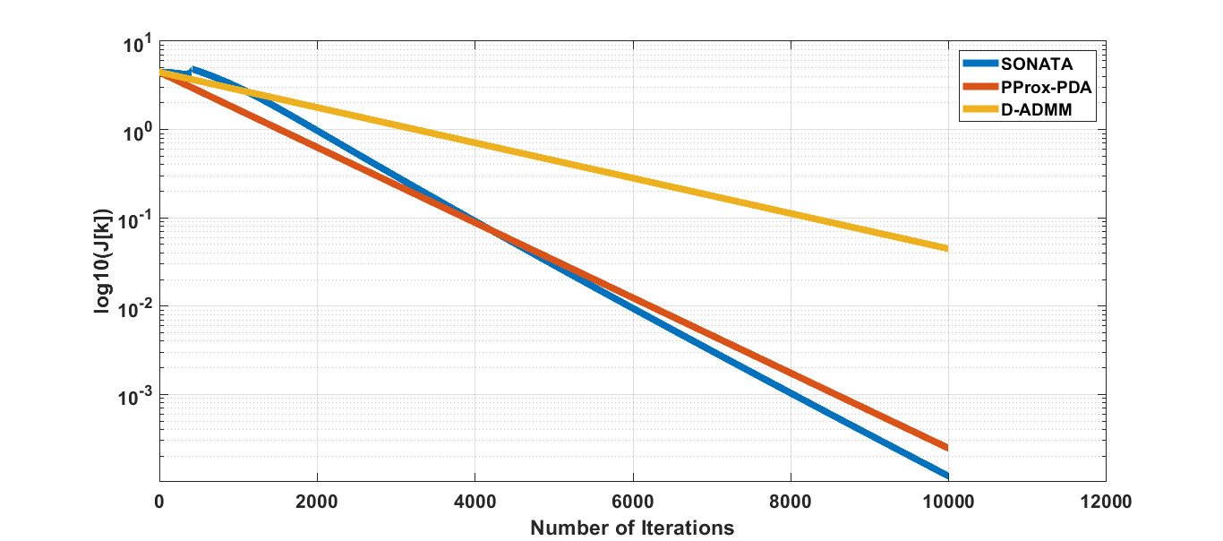
Figure 2: Decentralized PCA: Distance of the iterates from a stationary solution vs. iterations.

5.2 Sparse linear regression with $\ell_{1}$ regularization

Consider the decentralized LASSO problem using $\ell_{1}$ regularization, as described in Sec. 2.1.1(i). Data are generating according the following model. The ground truth ${x}^{*}\in\mathbb{R}^{350}$ is built first drawing randomly a vector from the normal distribution $N({0},{I}_{350})$, then thresholding the smallest 40% of its elements to $0$. The underlying linear model is ${y}_{i}={A}_{i}{x}^{*}+{w}_{i}$, where the observation matrix ${A}_{i}\in\mathbb{R}^{15\times 350}$ is generated by drawing i.i.d. elements from the distribution $N(0,1)$, and then normalizing the rows to unit norm; and ${w}_{i}$ is the additive noise vector with i.i.d. entries from $N(0,0.1)$. Finally the regularization parameter is set to $\lambda=2$. We contrast the SONATA algorithm (tuning parameter: $\alpha=0.015$) with the most popular decentralized algorithms proposed to solve convex, composite optimization problems, namely: (i) NIDS (tuning parameters: $\alpha=0.017$) [29], (ii) PG-EXTRA (tuning parameter: $\alpha=0.011$) [42], (iii) Distributed ADMM (tuning parameter: $\rho=4.2$) [20]. We also included the PProx-PDA (tuning parameters: $\gamma=10^{-4},\ \beta=24.21$) [18]. In Figure 3, we plot $\text{log}_{10}||{X}^{\nu}-1({x}^{*})^{\top}||$ versus the number of iterations $\nu$, where $x^{\star}$ is a solution of the LASSO problem. The figure confirms linear convergence of the SONATA algorihtm, given that the LASSO function is a KL function with exponent $\theta=1/2$. No such a theoretical result is available for the other decentralized algorithms.

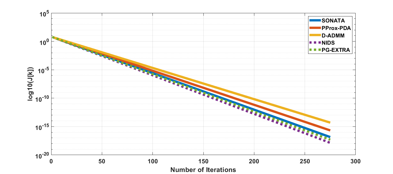
Figure 3: LASSO with $\ell_{1}$ regularization: distance of the iterates from a solution vs. iterations.

5.3 SCAD regularized distributed least squares

Consider now the sparse linear regression problem formulated as quadratic minimization with the SCAD regularization, as described in Sec. 2.1.1(ii). The data generation model is the following. The ground truth signal ${x}^{*}\in\mathbb{R}^{350}$ is built by first drawing randomly a vector from the normal distribution $\mathcal{N}({0},{I}_{350})$, then thresholding the smallest 20% of its elements to $0$. The underlying linear model is generated as for the example in Sec. 5.2.

The SONATA algorithm(with tuning: $\alpha=0.002$) is compared with the PProx-PDA (tuning parameter: $\gamma=10^{-4},\beta=30.23$) [18] and the Distributed ADMM (tuning parameter $\rho=2.5$) [20]. In Figure 4, we plot $\text{log}_{10}||{X}^{\nu}-1({x}^{*})^{\top}||$ versus the number of iterations $\nu$. All the algorithms are observed to converge to the same stationary solution. The figure confirms the same results as observed for the other classes of functions satisfying the KL property with exponent $\theta=1/2$.

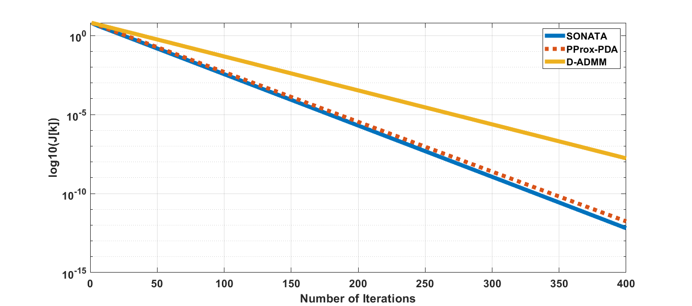
Figure 4: Sparse linear regression with SCAD regularization: Distance from stationarity vs. iterations.

6 Concluding Remarks

We provided a new line of analysis for the rate of convergence of the SONATA algorithm, to solve Problem (P), under the KL property of $u$. The established convergence rates match those obtained in the centralized scenario by the centralized proximal gradient algorithm, for different values of the exponent $\theta\in(0,1)$. When $\theta=0$, finite time convergence of the sequence (as for the proximal gradient algorithm in the centralized case) cannot be always guarantees, due to the perturbation induced by consensus errors. In such cases we still identified sufficient conditions under which the SONATA algorithm matches the behavior of the centralized proximal gradient. A future direction to address this issue would be devising decentralized designs that escape local maxima.

Appendix A Appendix for the rate analysis

This appendix contains some definitions and lemmata established in the literature, and used in our analysis of convergence rate. The proofs of the lemmata are presented for the sake of completeness.

Lemma 3.

For $x\in\mathbb{R}^{d}$ and $\theta\in(0,1)$, the following hold:

1. If $\theta\leq\frac{1}{2}$, then $\|x\|_{1/\theta}\leq\|x\|_{2}$;

2. If $\theta>\frac{1}{2}$, then $\|x\|_{1/\theta}\leq d^{\theta-1/2}\|x\|_{2}.$

Proof.

By the Hölder’s inequality, we have for any $0<r<p$,

$$\|x\|_{p}\leq\|x\|_{r}\leq d^{1/r-1/p}\|x\|_{p}.$$ (53)

The inequalities in (i) and (ii) follow from (53), setting therein $p={1}/{\theta}$ and $r=2$ for (i), and $p=2$, $r={1}/{\theta}$ for (i). ∎

Lemma 4 (Exponent for separable sums of KL functions).

Let $F(X)=\sum_{i=1}^{m}f_{i}(x_{i})$, where $f_{i}$ is a proper closed function on $\mathbb{R}^{d}$ and $X=[x_{1},x_{2},\cdots,x_{m}]^{\top}$. Suppose further that for each $i$, $f_{i}$ is continuous on $\text{dom}\partial f_{i}$ and satisfies KL property (Def. 1) at $\bar{x}_{i}$ with exponent $\theta\in[0,1)$ and parameters $(\kappa_{i},\eta_{i})$. Then $F$ satisfies KL property (Def. 1) at $\bar{X}=[\bar{x}_{1},\bar{x}_{2},\cdots,\bar{x}_{m}]^{\top}$ with exponent $\theta$ and parameters $(\kappa/\max\{d^{\theta-\frac{1}{2}},1\},1)$ with $\kappa=\max_{i}\kappa_{i}$.

Proof.

See the proof of Theorem 3.3 in [27] with minor variation and calculate the explicit expression of KL coefficient of $F$ using Lemma 3. ∎

Lemma 5.

For $0\leq b\leq a$, and $\theta<1$, we have that

$$a-b\leq\frac{1}{1-\theta}a^{\theta}(a^{1-\theta}-b^{1-\theta}).$$

Proof.

Define $\Phi(x):x^{1-\theta}$. Then, $\Phi^{\prime}(x)=(1-\theta)x^{-\theta}$ is decreasing for $x>0$. By mean value theorem, there exists $c\in[b,a]$ such that

$$\Phi(a)-\Phi(b)= \,\Phi^{\prime}(c)(a-b)\geq\Phi^{\prime}(a)(a-b).$$

$$\Rightarrow a-b\leq\frac{1}{1-\theta}a^{\theta}(a^{1-\theta}-b^{1-\theta}).\vskip-11.38092pt$$

∎

Lemma 6.

Consider Problem (P) under Assumption 1. Let $\{X^{\nu}\}_{\nu\in\mathbb{N}}$ be the sequence generated by the SONATA algorithm (7a)-(7c), under Assumption 2. Then there exists $G^{\nu}\in\partial U(X^{\nu+1/2})$ such that

$$\|G^{\nu}\|^{2}\leq 3\left(L^{2}+\frac{1}{\alpha^{2}}\right)\|D^{\nu}\|^{2}+3\mathcal{E}^{\nu}.$$

Proof.

By (7a), there exists $J^{\nu}\in\partial R(X^{\nu+1/2})$ such that

$$J^{\nu}+\frac{1}{\alpha}(X^{\nu+1/2}-X^{\nu}+\alpha Y^{\nu})=0.$$

That is, there exists $G^{\nu}\in\partial U(X^{\nu+1/2})$ such that

$$\|G^{\nu}\|^{2}= \sum_{i=1}^{m}\left\|\nabla f(x_{i}^{\nu+1/2})-y_{i}^{\nu}-\frac{1}{\alpha}(x_{i}^{\nu+1/2}-x_{i}^{\nu})\right\|^{2}$$

$$\leq 3\left(L^{2}+\frac{1}{\alpha^{2}}\right)\|D^{\nu}\|^{2}+3\mathcal{E}^{\nu}.$$

∎

Lemma 7 (Th. 2 in [3]).

Let $\{\mathcal{S}^{\nu}\}$ be a nonnegative sequence satisfying

$$(\mathcal{S}^{\nu})^{\frac{\theta}{1-\theta}}\leq c(\mathcal{S}^{\nu-1}-\mathcal{S}^{\nu}),\quad\forall\nu\geq\nu_{0},$$

there exists $c^{\prime}>0$ such that

$$\mathcal{S}^{\nu}\leq c^{\prime}\nu^{-\frac{1-\theta}{2\theta-1}},\quad\forall\nu\geq\nu_{0}.$$

Appendix B Appendix for the KL property

This appendix introduces a stronger version of KL property than that in Definition 2, which allows SONATA to match the convergence rate results of the centralized proximal gradient, when the KL exponent of $u$ (according to Definition 2) is zero. Specifically, we have the following.

Definition 2.

(A stronger version of the KL property)[37] A proper closed function $f$ satisfies the KL property at $\bar{x}\in\text{dom}f$ with exponent $\theta\in[0,1)$ if there exists a neighborhood $E$ of $\bar{x}$ and numbers $\kappa,\eta\in(0,\infty)$ such that

$$\|g_{x}\|\geq\kappa|f(x)-f(\bar{x})|^{\theta},$$ (54)

for all $x\in E\cap[f(\bar{x})-\eta<f<f(\bar{x})+\eta]$ and $g_{x}\in\partial f(x)$. We call the function $f$ a KL function with exponent $\theta$ if it satisfies the KL property at any point $\bar{x}\in\text{dom}\partial f$ with the same exponent $\theta$.

The relationship with the original KL property in Definition 1 follows readily.

Remark 1.

If a function $f$ is proper and closed. Then $f$ satisfies KL property (Def. 2) at $\bar{x}\in\text{dom}\partial f$ with exponent $\theta\in[0,1)$ if and only if both $f$ and $-f$ satisfy the original KL property (Def. 1) at $\bar{x}$ with some exponents $\theta_{1},\theta_{2}\in[0,1)$ respectively, where $\theta=\max\{\theta_{1},\theta_{2}\}$.

Several functions satisfy such a KL property.

Proposition 1.

Let $f$ be a proper and closed sub-analytic function with closed domain, then $f$ is a KL function with exponent $\theta\in[0,1)$.

Proof.

By in [10, Th. 3.1], both $f$ and $-f$ satisfy the original KL property (Def. 1) at each $x\in\text{dom}\partial f$ with a $\theta\in[0,1)$. ∎

Furthermore, such a stronger version of the KL inherits most of the desirable properties of that in Definition 1, including exponent-preserving rules such as composition rule [27, Thm 3.2], minimum rule [27, Thm 3.1] and rule of separable sums[27, Thm 3.3]. To be concrete, with the help of several intermediate properties (Lemma 8, 9, 10) proved below, we provide next two classes of functions satisfying Definition 2 with exponent $\theta=1/2$ (see Theorem 3 and Theorem 4 below). This also shows that all the illustrative examples discussed in Sec. 2.1.1 satisfy Definition 2 with the same exponents $\theta$ as in Definition 1 (see Remark 2).

Unless otherwise specified, in the following when calling the KL property (or a KL function), we refer to to the stronger Definition 2.

Lemma 8.

Suppose $f$ is a proper closed function, $\bar{x}\in\text{dom}$ $\partial f$ and $\bar{x}$ is not a stationary point ($0\notin\partial f(\bar{x})$). Then for any $\theta\in[0,1)$, $f$ satisfies the KL property at $\bar{x}$ with exponent $\theta$.

Proof.

See Lemma 2.1 in [27] with a minor variation. ∎

Definition 3 (Luo-Tseng Error Bound).

[27, Def 2.1] Consider Problem (P). Let $\mathcal{X}$ be the set of stationary points of $u$. Suppose $\mathcal{X}\neq\emptyset$. We say that the Luo-Tseng error bound holds if for any $\zeta>\inf u$, there exists $c_{1},\epsilon_{1}>0$ such that whenever $\|\texttt{prox}_{r}(x-\nabla f(x))-x\|<\epsilon_{1}$ and $u(x)<\zeta$,

$$\text{dist}(x,\mathcal{X})\leq c_{1}\|\texttt{prox}_{r}(x-\nabla f(x))-x\|$$

Lemma 9 (Luo-Tseng error bound implies KL).

Consider the problem (P) under Assumption 1. Suppose that the set $\mathcal{X}$ of stationary points of Problem (P) is nonempty and for any $x^{*}\in\mathcal{X}$, there exists $\delta>0$ such that $u(x)=u(x^{*})$ whenever $x\in\mathcal{X}$ and $\|x-x^{*}\|\leq\delta$. If the Luo-Tseng error bound holds for $u$, then $u$ is a KL function with exponent $\theta={1}/{2}$.

Proof.

It follows for the proof of [27, Th. 4.1] with minor variations. ∎

Lemma 10 (Exponent of the minimum of finitely many KL functions).

Let $f_{i}$, $1\leq i\leq r$, be proper closed function with $\text{dom}f_{i}=\text{dom}$ $\partial f_{i}$ for all $i$, and $f:=\min_{1\leq i\leq r}f_{i}$ be continuous on $\text{dom}\partial f$. Suppose further that each $f_{i}$ is a KL function with exponent $\theta_{i}\in[0,1)$ for $1\leq i\leq r$. Then $f$ is also a KL function with exponent $\theta=\max\{\theta_{i}:1\leq i\leq r\}$.

Proof.

The proof follows similar steps as that in [27, Cor. 3.1]. ∎

We are ready to state the two major results of this section.

Theorem 3 (Convex problems with convex piecewise linear-quadratic regularizers).

Suppose $u$ is a proper closed function taking the form

$$u(x)=\min_{1\leq r\leq r}\underbrace{l(Ax)+r_{i}(x)}_{u_{i}(x)},$$

where $A\in\mathbb{R}^{m\times n}$, $r_{i}$ are proper closed polyhedral functions for $i=1,\cdots,r$ and $l$ satisfies either one of the following two conditions:

• $l$ is a proper closed convex function with an open domain, and is strongly convex on any compact convex subset of $\text{dom}\,l$ and is twice continuously differentiable on $\text{dom}\,l$;

• $l(y)=\max_{z\in D}\left\{\right\langle y,z\rangle-q(z)\}$ for all $y\in\mathbb{R}^{m}$, with $D$ being a polyhedron and $q$ being a strongly convex differentiable function with a Lipschitz continuous gradient.

Suppose in addition that $f$ is continuous on dom $\partial u$, then $u$ is a KL function with exponent $1/2$.

Proof.

Following the analysis in [27, Cor. 5.1], one can show that, for each $i$, $u_{i}$ satisfies all the assumptions in Proposition 9, and $\text{dom}u_{i}=\text{dom}\,\partial u_{i}.$ The proof follows then by Proposition 8 (for the case argmin $u_{i}=\emptyset$), Lemma 9 and Lemma 10. ∎

Theorem 4 (nonconvex minimum-of-quadratic regularizers).

Consider the following class of functions

$$u(x)=\min_{1\leq i\leq r}\underbrace{\left\{\frac{1}{2}x^{\top}A_{i}x+b_{i}^{\top}x+\beta_{i}+r_{i}(x)\right\}}_{u_{i}(x)},$$

where $r_{i}$ are proper closed polyhedral functions, $A_{i}\in\mathbb{R}^{n\times n}$ is symmetric, $b_{i}\in\mathbb{R}^{n}$ and $\beta_{i}\in\mathbb{R}^{n}$ for $i=1,\cdots,r$. Suppose, in addition, that $u$ is continuous on $\text{dom}\,\partial u$. Then $u$ is a KL function with exponent $1/2$.

Proof.

Following the analysis in [27, Cor. 5.2], we have that, for each $i$, $u_{i}(x)$ satisfies all assumptions in Proposition 9 and $\text{dom}u_{i}=\text{dom}\partial u_{i}.$ Then, the proof follows combining Proposition 8 (for the case argmin $u_{i}=\emptyset$), 9 with Lemma 10. ∎

Remark 2.

By Theorem 3, we have that objective functions in the example (i) and (iii) in Sec. 2.1.1 are KL functions with exponent $\theta=1/2$. By Theorem 4, we have that objective functions of the example (ii) and (iv) in Sec. 2.1.1 are KL functions with exponent $\theta=1/2$. Objective function of example (v) in Sec. 2.1.1 is a KL function with exponent $1/2$, as it satisfies the even stronger gradient dominance condition in [52, Def.1]. Finally, by Proposition 1, the objective function of example (vi) in Sec 2.1.1 is a KL function with $\theta\in[0,1)$. This proves our claim that all the examples listed in Sec 2.1.1 share the same exponent $\theta$ in both definitions (Def. 1 and Def. 2).

References

- [1] Pierre-Antoine Absil, Robert Mahony, and Ben Andrews. Convergence of the iterates of descent methods for analytic cost functions. SIAM Journal on Optimization, 16(2):531–547, 2005.
- [2] Miju Ahn, Jong-Shi Pang, and Jack Xin. Difference-of-convex learning: directional stationarity, optimality, and sparsity. SIAM Journal on Optimization, 27(3):1637–1665, 2017.
- [3] Hedy Attouch and Jérôme Bolte. On the convergence of the proximal algorithm for nonsmooth functions involving analytic features. Mathematical Programming, 116:5–16, 2009.
- [4] Hédy Attouch, Jérôme Bolte, Patrick Redont, and Antoine Soubeyran. Proximal alternating minimization and projection methods for nonconvex problems: An approach based on the kurdyka-łojasiewicz inequality. Mathematics of operations research, 35(2):438–457, 2010.
- [5] Hedy Attouch, Jérôme Bolte, and Benar Fux Svaiter. Convergence of descent methods for semi-algebraic and tame problems: proximal algorithms, forward–backward splitting, and regularized gauss–seidel methods. Mathematical Programming, 137(1):91–129, 2013.
- [6] Winfried Auzinger and J Melenk. Iterative solution of large linear systems. Lecture notes, TU Wien, 2011.
- [7] GC Bento, BS Mordukhovich, TS Mota, and Yu Nesterov. Convergence of descent methods under kurdyka-l ojasiewicz properties. arXiv preprint arXiv:2407.00812, 2024.
- [8] Raphael Berthier, Francis Bach, and Pierre Gaillard. Accelerated gossip in networks of given dimension using jacobi polynomial iterations. SIAM J. on Mathematics of Data Science, 1:24–47, 2020.
- [9] Pascal Bianchi and Jérémie Jakubowicz. Convergence of a multi-agent projected stochastic gradient algorithm for non-convex optimization. IEEE transactions on automatic control, 58(2):391–405, 2012.
- [10] Jérôme Bolte, Aris Daniilidis, and Adrian Lewis. The łojasiewicz inequality for nonsmooth subanalytic functions with applications to subgradient dynamical systems. SIAM Journal on Optimization, 17(4):1205–1223, 2007.
- [11] Jérôme Bolte, Aris Daniilidis, Olivier Ley, and Laurent Mazet. Characterizations of łojasiewicz inequalities: subgradient flows, talweg, convexity. Transactions of the American Mathematical Society, 362(6):3319–3363, 2010.
- [12] Jérôme Bolte, Shoham Sabach, and Marc Teboulle. Proximal alternating linearized minimization for nonconvex and nonsmooth problems. Mathematical Programming, 146(1):459–494, 2014.
- [13] Loris Cannelli. Asynchronous Parallel Algorithms for Big-Data Nonconvex Optimization. PhD thesis, Purdue University Graduate School, 2019.
- [14] Amir Daneshmand, Gesualdo Scutari, and Vyacheslav Kungurtsev. Second-order guarantees of distributed gradient algorithms. SIAM Journal on Optimization, 30(4):3029–3068, 2020.
- [15] Paolo Di Lorenzo and Gesualdo Scutari. Distributed nonconvex optimization over networks. In 2015 IEEE 6th International Workshop on Computational Advances in Multi-Sensor Adaptive Processing (CAMSAP), pages 229–232. IEEE, 2015.
- [16] Paolo Di Lorenzo and Gesualdo Scutari. Next: In-network nonconvex optimization. IEEE Transactions on Signal and Information Processing over Networks, 2(2):120–136, 2016.
- [17] Pierre Frankel, Guillaume Garrigos, and Juan Peypouquet. Splitting methods with variable metric for kurdyka–łojasiewicz functions and general convergence rates. Journal of Optimization Theory and Applications, 165:874–900, 2015.
- [18] Davood Hajinezhad and Mingyi Hong. Perturbed proximal primal–dual algorithm for nonconvex nonsmooth optimization. Mathematical Programming, 176(1):207–245, 2019.
- [19] Mingyi Hong, Davood Hajinezhad, and Ming-Min Zhao. Prox-pda: The proximal primal-dual algorithm for fast distributed nonconvex optimization and learning over networks. In International Conference on Machine Learning, pages 1529–1538. PMLR, 2017.
- [20] Mingyi Hong, Zhi-Quan Luo, and Meisam Razaviyayn. Convergence analysis of alternating direction method of multipliers for a family of nonconvex problems. SIAM Journal on Optimization, 26(1):337–364, 2016.
- [21] Mingyi Hong, Siliang Zeng, Junyu Zhang, and Haoran Sun. On the divergence of decentralized nonconvex optimization. SIAM Journal on Optimization, 32(4):2879–2908, 2022.
- [22] Chi Jin, Rong Ge, Praneeth Netrapalli, Sham M Kakade, and Michael I Jordan. How to escape saddle points efficiently. In International conference on machine learning, pages 1724–1732. PMLR, 2017.
- [23] Krzysztof Kurdyka. On gradients of functions definable in o-minimal structures. In Annales de l’institut Fourier, volume 48, pages 769–783, 1998.
- [24] Tim Tsz-Kit Lau, Jinshan Zeng, Baoyuan Wu, and Yuan Yao. A proximal block coordinate descent algorithm for deep neural network training. arXiv preprint arXiv:1803.09082, 2018.
- [25] Jason D Lee, Ioannis Panageas, Georgios Piliouras, Max Simchowitz, Michael I Jordan, and Benjamin Recht. First-order methods almost always avoid strict saddle points. Mathematical programming, 176:311–337, 2019.
- [26] Jason D Lee, Max Simchowitz, Michael I Jordan, and Benjamin Recht. Gradient descent only converges to minimizers. In Conference on learning theory, pages 1246–1257. PMLR, 2016.
- [27] Guoyin Li and Ting Kei Pong. Calculus of the exponent of kurdyka–łojasiewicz inequality and its applications to linear convergence of first-order methods. Foundations of computational mathematics, 18(5):1199–1232, 2018.
- [28] Qunwei Li, Yi Zhou, Yingbin Liang, and Pramod K Varshney. Convergence analysis of proximal gradient with momentum for nonconvex optimization. In International Conference on Machine Learning, pages 2111–2119. PMLR, 2017.
- [29] Zhi Li, Wei Shi, and Ming Yan. A decentralized proximal-gradient method with network independent step-sizes and separated convergence rates. IEEE Transactions on Signal Processing, 67(17):4494–4506, 2019.
- [30] Shu Liang, George Yin, et al. Exponential convergence of distributed primal–dual convex optimization algorithm without strong convexity. Automatica, 105:298–306, 2019.
- [31] Huikang Liu, Anthony Man-Cho So, and Weijie Wu. Quadratic optimization with orthogonality constraint: explicit łojasiewicz exponent and linear convergence of retraction-based line-search and stochastic variance-reduced gradient methods. Mathematical Programming, 178(1):215–262, 2019.
- [32] Stanislaw Lojasiewicz. Une propriété topologique des sous-ensembles analytiques réels. Les équations aux dérivées partielles, 117:87–89, 1963.
- [33] A. Nedić, A. Olshevsky, and M. G. Rabbat. Network topology and communication-computation tradeoffs in decentralized optimization. Proceedings of the IEEE, 106:953–976, September 2018.
- [34] Peter Ochs, Yunjin Chen, Thomas Brox, and Thomas Pock. ipiano: Inertial proximal algorithm for nonconvex optimization. SIAM Journal on Imaging Sciences, 7(2):1388–1419, 2014.
- [35] SH Pan and YL Liu. Metric subregularity of subdifferential and kl property of exponent 1/2. arXiv preprint arXiv:1812.00558, 2019.
- [36] Yitian Qian and Shaohua Pan. Convergence of a class of nonmonotone descent methods for kurdyka–łojasiewicz optimization problems. SIAM Journal on Optimization, 33(2):638–651, 2023.
- [37] Junwen Qiu, Bohao Ma, Xiao Li, and Andre Milzarek. A kl-based analysis framework with applications to non-descent optimization methods. arXiv preprint arXiv:2406.02273, 2024.
- [38] RT Rockafellar and RJB Wets. Variational analysis springer-verlag. New Y ork, 1998.
- [39] Kevin Scaman, Francis Bach, Sébastien Bubeck, Yin Tat Lee, and Laurent Massoulié. Optimal algorithms for smooth and strongly convex distributed optimization in networks. In international conference on machine learning, pages 3027–3036. PMLR, 2017.
- [40] Gesualdo Scutari and Ying Sun. Distributed nonconvex constrained optimization over time-varying digraphs. Mathematical Programming, 176:497–544, 2019.
- [41] Wei Shi, Qing Ling, Gang Wu, and Wotao Yin. Extra: An exact first-order algorithm for decentralized consensus optimization. SIAM Journal on Optimization, 25(2):944–966, 2015.
- [42] Wei Shi, Qing Ling, Gang Wu, and Wotao Yin. A proximal gradient algorithm for decentralized composite optimization. IEEE Transactions on Signal Processing, 63(22):6013–6023, 2015.
- [43] Ying Sun, Gesualdo Scutari, and Amir Daneshmand. Distributed optimization based on gradient tracking revisited: Enhancing convergence rate via surrogation. SIAM Journal on Optimization, 32(2):354–385, 2022.
- [44] Hanlin Tang, Xiangru Lian, Ming Yan, Ce Zhang, and Ji Liu. D2: Decentralized training over decentralized data. In International Conference on Machine Learning, pages 4848–4856. PMLR, 2018.
- [45] Tatiana Tatarenko and Behrouz Touri. Non-convex distributed optimization. IEEE Transactions on Automatic Control, 62(8):3744–3757, 2017.
- [46] Ye Tian, Ying Sun, and Gesualdo Scutari. Asynchronous decentralized successive convex approximation. arXiv preprint arXiv:1909.10144, 2019.
- [47] Hoi-To Wai, Jean Lafond, Anna Scaglione, and Eric Moulines. Decentralized frank–wolfe algorithm for convex and nonconvex problems. IEEE Transactions on Automatic Control, 62(11):5522–5537, 2017.
- [48] Lin Xiao, Stephen Boyd, and Sanjay Lall. A scheme for robust distributed sensor fusion based on average consensus. In IPSN 2005. Fourth International Symposium on Information Processing in Sensor Networks, 2005., pages 63–70. IEEE, 2005.
- [49] Xinlei Yi, Shengjun Zhang, Tao Yang, Tianyou Chai, and Karl H Johansson. Exponential convergence for distributed optimization under the restricted secant inequality condition. IFAC-PapersOnLine, 53(2):2672–2677, 2020.
- [50] Xinlei Yi, Shengjun Zhang, Tao Yang, Tianyou Chai, and Karl H Johansson. Linear convergence of first-and zeroth-order primal–dual algorithms for distributed nonconvex optimization. IEEE Transactions on Automatic Control, 67(8):4194–4201, 2021.
- [51] Jinshan Zeng and Wotao Yin. On nonconvex decentralized gradient descent. IEEE Transactions on signal processing, 66(11):2834–2848, 2018.
- [52] Yi Zhou and Yingbin Liang. Characterization of gradient dominance and regularity conditions for neural networks. arXiv preprint arXiv:1710.06910, 2017.
- [53] Minghui Zhu and Sonia Martínez. An approximate dual subgradient algorithm for multi-agent non-convex optimization. IEEE Transactions on Automatic Control, 58(6):1534–1539, 2012.
- [54] Sanjo Zlobec. Jensen’s inequality for nonconvex functions. Mathematical Communications, 9(2):119–124, 2004.