Black Mirrors: CPT-Symmetric Alternatives to Black Holes
Abstract
Einstein’s equations imply that a gravitationally collapsed object forms an event horizon. But what lies on the other side of this horizon? In this paper, we question the reality of the conventional solution (the black hole), and point out another, topologically distinct solution: the black mirror. In the black hole solution, the horizon connects the exterior metric to an interior metric which contains a curvature singularity. In the black mirror, the horizon instead connects the exterior metric to its own CPT mirror image, yielding a solution with no curvature singularities. We give the general stationary (charged, rotating) black mirror solution explicitly, and also describe the general black mirror formed by gravitational collapse. The black mirror is the relevant stationary point when the quantum path integral is equipped with suitably CPT-symmetric boundary conditions, that we propose. It appears to avoid many vexing puzzles which plague the conventional black hole.
I Introduction
The Einstein-Rosen bridge (the first wormhole geometry) was put forth by Einstein and Rosen in Einstein and Rosen (1935). One of their motivations was to get rid of the apparent “singularity” at the event horizon by introducing a new coordinate by , and letting extend over . This describes two Schwarzschild exteriors (regions and in Fig. 1a), glued at the radius (the midpoint in Fig. 1a). However, it was later deemed to be unphysical as the papers of Oppenheimer-Snyder Oppenheimer and Snyder (1939) describing spherical collapse showed that the singularity at is just a coordinate singularity, and an infalling observer following the collapsing matter will not feel anything unusual happening at the event horizon. This (and other developments) led to the modern belief that the black hole interior really exists, and that the black hole’s horizon is completely non-singular.
Nevertheless, the modern black hole picture of gravitational collapse is not without its problems. Aside from the emergence of curvature singularities, there are other problems that the currently accepted theories cannot address adequately, including the breakdown of causality, i.e., the emergence and stability of Cauchy horizons Dafermos and Luk (2017), as well as the information Hawking (1976) and firewall Almheiri et al. (2013) paradoxes.
In this paper, we argue that certain natural modifications of Einstein-Rosen bridges – which we call black mirrors – are, in fact, direct consequences of CPT symmetry, and offer novel solutions to the problems mentioned above, along with other merits discussed below.111We also draw the reader’s attention to several other proposals for variations to the usual black hole geometry or topology Gibbons (1986); Saravani et al. (2015); Visser (1989a, b); ’t Hooft (2016, 2017).
II The Schwarzschild black mirror
For simplicity, let us first consider the Schwarzschild metric, describing an eternal, static, uncharged object. In Schwarzschild coordinates it is
| (1) |
where
| (2) |
This solution has a horizon at , the root of . Note that Schwarzschild coordinates only cover the exterior region , and become singular at the horizon (which lies at in these coordinates).
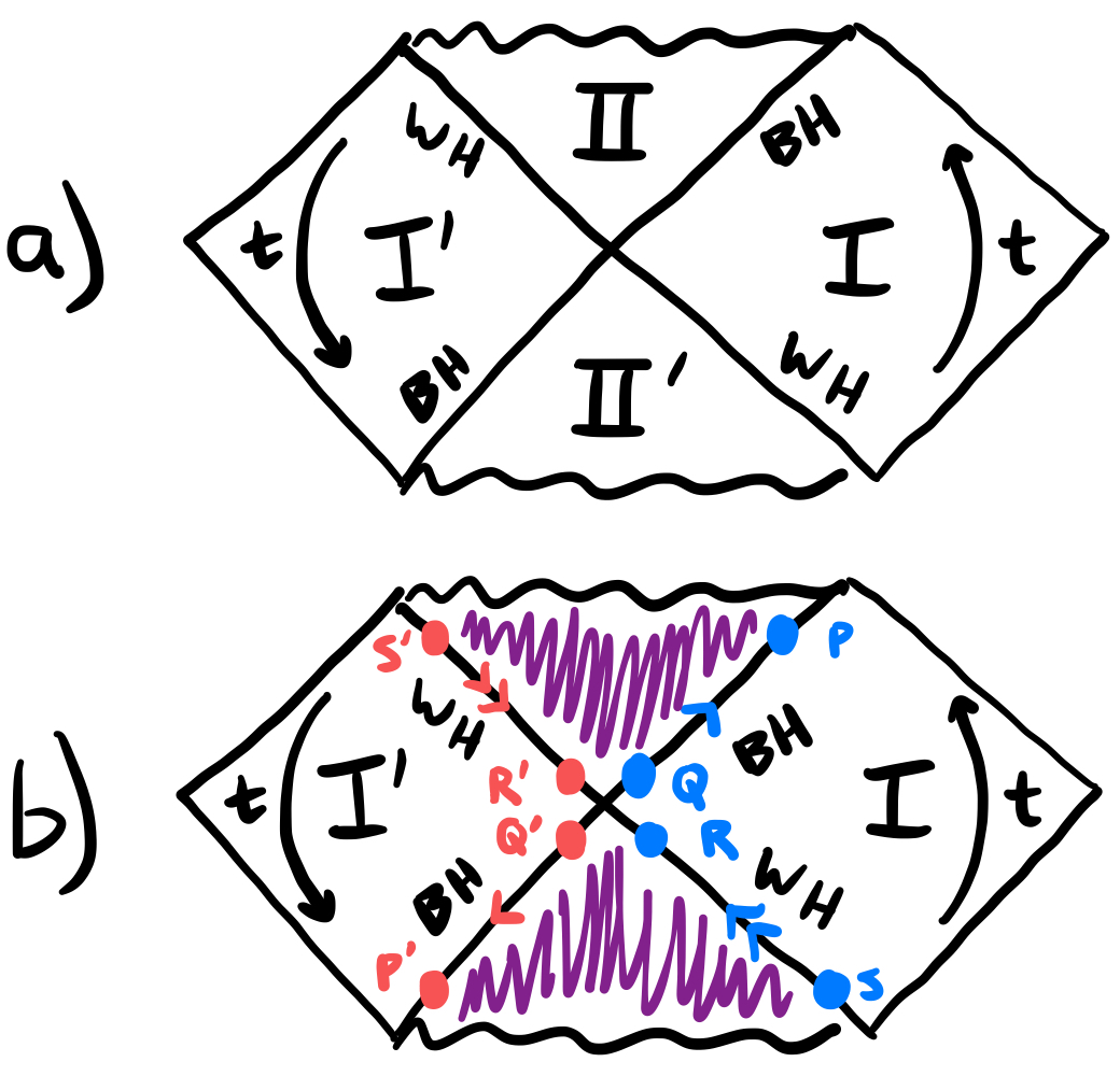
The conventional view is that the full spacetime (including the horizon, and what lies behind it) is the maximal analytic extension obtained by switching from Schwarzschild to Kruskal coordinates d’Invemo (1992). The Penrose diagram of this extension is shown in Fig. 1a: it has two exterior regions , , two interior regions , , two black horizons (BHs) that particles can only enter, and two white horizons (WHs) that particles can only exit.
The simplest coordinate system that non-singularly covers both the exterior and its BH (WH) is the ingoing (outgoing) Eddington-Finkelstein system, in which we replace Schwarzschild time by ingoing (outgoing) Eddington-Finkelstein time (), related by , so that the line element (1) becomes
| (3) |
Following the classic Gibbons-Hawking analysis Gibbons and Hawking (1977), in order to extract the quantum/thermodynamic properties of this spacetime, and to define quantum field theory on it, it is standard to start in Schwarzschild coordinates (the coordinates that make manifest the full isometry group of the metric) and then “Wick rotate” to the Euclidean Schwarzschild metric, by replacing the Schwarzschild coordinates, and , by the Euclidean time and Euclidean radius , defined by
| (4) |
So the Euclidean Schwarzschild metric (in coordinates) is given by
| (5) |
For small (which corresponds to the near-horizon limit in Lorentzian signature), this becomes
| (6) |
One recognizes this as the metric of a 2-dimensional () cone , with a 2-dimensional () sphere of radius living over each point of the cone (see Fig. 2a). The has angular coordinate , and radial coordinate measuring the proper distance from the tip . Note that, in the standard Euclidean analysis Gibbons and Hawking (1977), one considers the one-sided (the blue cone in Fig. 2a), corresponding to the black hole exterior region ().
Then, if the Euclidean time coordinate’s period is precisely (i.e. if we identify ), the conic singularity at is removed, and the one-sided (the blue cone in Fig. 2a) becomes a non-singular 2D Euclidean surface (the blue surface in Fig. 2b). From this, one infers that the black hole’s temperature is the inverse of this natural period: Gibbons and Hawking (1977).
After this elegant argument, we appear to be left with a smooth, complete Euclidean spacetime (the blue surface in Fig. 2b) which is usually regarded as the entire Euclidean Schwarzschild metric. But this blue surface corresponds purely to the Schwarzschild exterior (region in Fig. 1a). What happened to the spacetime behind the event horizon at ?
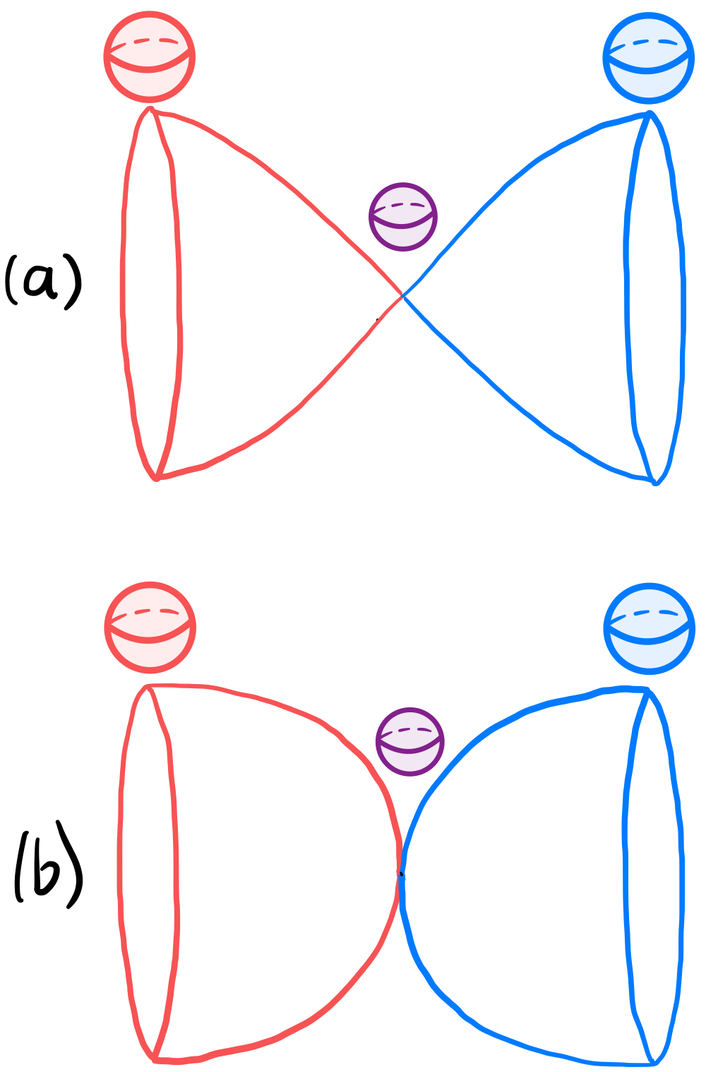
To answer this question, let us first take a step back to the conical geometry of Fig. 2a. Here it is clear that the single (blue) cone naturally extends to the double (blue+red cone) by letting extend to negative values. Then, when we identify (removing the conical singularity), we obtain the full (blue+red) Euclidean Schwarzschild metric, Fig. 2b. Note: this full geometry still has nothing corresponding to the black hole interior; instead, it has two exteriors glued together at (an of area , corresponding to the horizon).
Further evidence for the two-sided geometry in Fig. 2b comes from black hole entropy. Gibbons and Hawking Gibbons and Hawking (1977) compute the entropy of the Schwarzschild black hole by computing the action of the Euclidean Schwarzschild metric (which comes entirely from the Gibbons-Hawking-York boundary term York (1972); Gibbons and Hawking (1977)). And, because they compute this action for the one-sided (blue) spacetime, they obtain a non-zero answer. This is a clue that the one-sided Euclidean metric is physically incomplete. If, instead, we compute the action/entropy for the two-sided Euclidean spacetime, the answer vanishes (as the two boundary terms, on isometric but oppositely oriented boundaries, make equal and opposite contributions, see Appendix B). This suggests a picture in which the full (blue+red) geometry corresponds to the full (pure, zero entropy) quantum state, while the half (blue) geometry corresponds to the mixed state obtained by tracing out the other (red) half; and the black hole entropy corresponds to the entanglement entropy (i.e. the von Neumann entropy of the blue side, after tracing out the red side). This in turn explains why the entropy is proportional to the area of the horizon (since the entanglement entropy between two regions is characteristically proportional to the size of the boundary separating them).
If we Wick rotate the full Euclidean metric (5) back to Lorentzian signature using , we obtain a metric that now covers the full exterior in Fig. 1a (i.e. regions and ). This is the Einstein-Rosen bridge Einstein and Rosen (1935), which is incomplete as it stands, and needs to be extended to a complete spacetime. The conventional completion is the Kruskal extension of Fig. 1a; but here we suggest a different completion. The simplest way to introduce this alternative possibility is to extend the metric to the horizon by replacing , as before, with the ingoing (outgoing) Eddington-Finkelstein time coordinate (). Then the metric becomes
| (7) |
Now notice that, in order for this extension to be well-defined (to not assign the same coordinate to two distinct points), we are forced (as shown in Fig. 1b) to identify the two BH horizons (e.g. ) and similarly the two WH horizons (e.g. ).222Note that we do not identify all antipodal pairs in Fig. 1a, as has sometimes been considered in the past Gibbons (1986); in particular, we do not identify points in exterior with points in exterior . This has the effect of gluing the exterior directly to the exterior , which together form a complete spacetime.
The resulting spacetime is the simplest (Schwarzschild) black mirror: eternal, static, uncharged. It is described by the metric (7), with and . More precisely, the ingoing (outgoing) Eddington-Finkelstein coordinates () cover the whole spacetime except the WH (BH), and these two coordinate systems together form a complete atlas. We see that, in coordinates, all components of the metric are explicitly smooth, analytic and finite functions of (for all ); and one can check that all associated curvature tensors and invariants (such as the Kretschmann scalar) are as well.
Note that the Lorentzian and Euclidean geometries are now in perfect correspondence: in both, the surface (i.e. the origin of the double cone in Euclidean signature, or the event horizon in Lorentzian signature) serves as the boundary between two mirror-image exterior regions, with no interior regions or curvature singularities.
But there is no free lunch! Although we have gotten rid of all curvature singularities, they have been replaced by another (milder) singularity. In particular, if we compute the eigenvalues of (in coordinates) then, in addition to the angular eigenvalues and , we see the remaining two (positive and negative) eigenvalues
| (8) |
swap places across the horizon, ; so both have simple analytic zeros at (while the corresponding eigenvalues of have simple poles).
In the standard black hole solution, we are used to the fact that, if some eigenvalues of approach zero or infinity as we approach the horizon, this is a mere coordinate singularity that can be removed by an appropriate change of coordinates. But in the black mirror, this is not possible – in coordinates where the metric is smooth and continuous across the horizon, the simple zeros in two eigenvalues of are unavoidable: they represent a genuine (but mild) singularity in the geometry, closely related to the singularity joining the two sides of the Euclidean Schwarzschild spacetime in Fig. 2b; and the corresponding simple poles in represent real phenomena, akin to the poles we go around in defining the Feynman propagator. We will explain their meaning below.
But first note that, although we have so far focused for simplicity on the Schwarzschild (i.e. 4D non-rotating, non-charged, asymptotically flat) black mirror, all the analysis and discussion extends directly – without any qualitative changes – to the most general 4D stationary black mirror (including rotation, electric and magnetic charge, and a non-zero cosmological constant). This is explained in detail in Appendix A. One can similarly obtain the spinning (A)dS black mirror in arbitrary dimensions, starting from the solution in Gibbons et al. (2004, 2005).
III Discussion
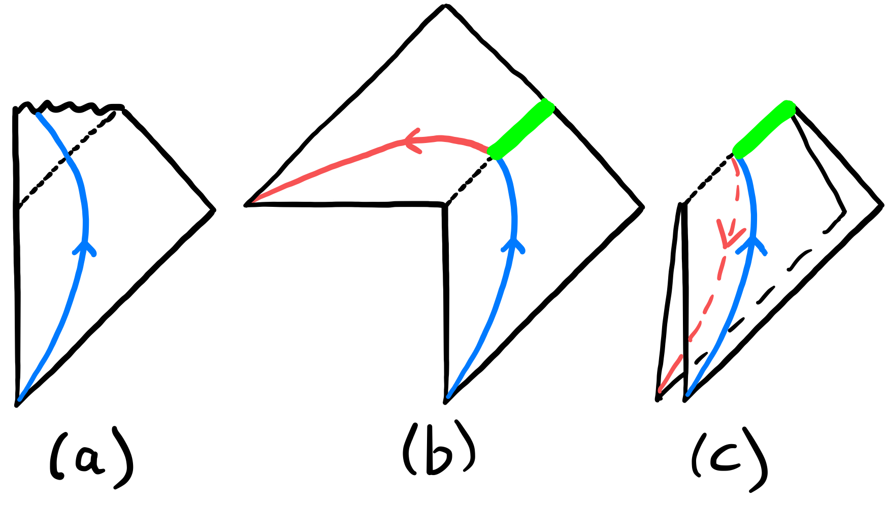
So far, we have considered the general stationary black mirror. Now let us explain how we think the general time-dependent case works. (Since this part of the story can no longer be described explicitly analytically, it is correspondingly less certain and more speculative.) We start with the Penrose diagram in Fig. 3a for an asymptotically-flat black hole formed by realistic gravitational collapse, with a blue curve showing the trajectory of an infalling particle (the arrow shows the direction of flow of electric charge). The corresponding black mirror is again obtained by identifying two CPT mirror copies of the exterior at their respective horizons, as in Fig. 3b: now we see that the (blue) particle falling into the BH from one side meets its CPT mirror (red) anti-particle falling in from the other side. For visualization, it is convenient to fold the diagram in Fig. 3b to obtain the diagram shown in Fig. 3c. In this folded picture, time runs in its usual upward direction on both sheets, and we can explicitly see that both sheets share a common future null boundary (i.e., a BH).
In the stationary case, the event horizon and apparent horizon coincide. More generally, where they do not, we conjecture the correct matching surface is the apparent horizon (which is well-defined to linear order in perturbations around the stationary solution Hollands et al. (2024)) since: (i) it is defined locally (unlike the event horizon); and (ii) it appears to be the surface associated to dynamical black hole entropy Hollands et al. (2024) which, as argued above, is also naturally associated to the surface separating the two exteriors of a black mirror. This suggests the potential, at least in principle, of observationally distinguishing dynamical black mirrors from dynamical black holes, e.g. via gravitational wave observations.
Finally, some further hints favoring black mirrors:
i) It is natural to consider the path integral for our universe with CPT-symmetric boundary conditions as shown in Fig. 6 (see Appendices B, C). Whereas the black hole (Fig. 1a) and black mirror (Fig. 1b) both satisfy these boundary condition, the black mirror seems to be the relevant saddle point as it (i) is free of curvature singularities, and (ii) has no additional boundaries (whereas the black hole solution has additional boundaries which are singular and also require further data to be specified).
ii) According to an external observer, an infalling object appears to take infinitely long to reach the BH. In the standard account Oppenheimer and Snyder (1939), this is an optical illusion: the infalling object actually crosses the horizon into the interior, but it takes infinitely long for the visual evidence to reach the exterior observer. However, taking quantum effects into account, the external observer sees the BH evaporate in a finite time, before the infalling object reaches the horizon, contradicting the standard account and drawing the interior’s existence into question Vachaspati et al. (2007); Vachaspati and Stojkovic (2008); Kawai et al. (2013).
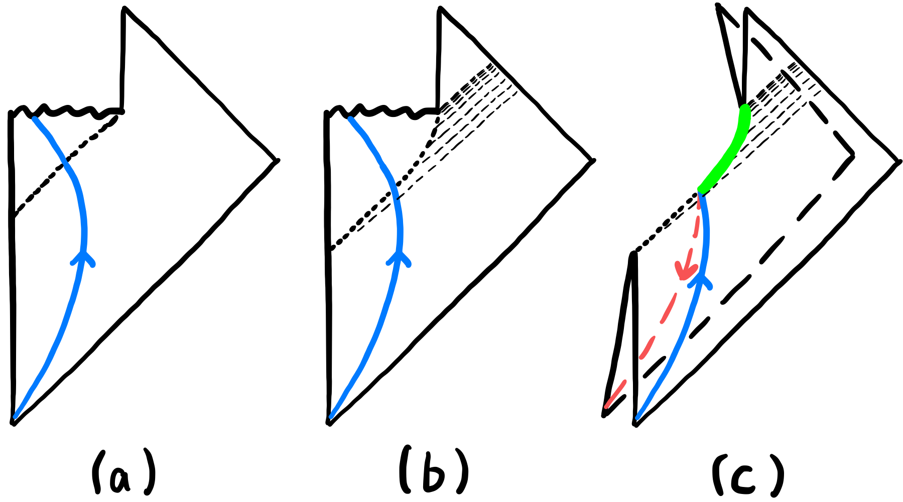
iii) The black hole information paradox Hawking (1976) and firewall paradox Almheiri et al. (2013) come from imagining that quantum information falls into a black hole, and asking how it can re-emerge (particularly since the black hole interior is causally disconnected from future null infinity, see Figs. 3a, 4a). In the black mirror Fig. 3c, with no interior, the puzzle is resolved: when a (blue) particle and (red) anti-particle meet at the horizon, they annihilate into (green) radiation that propagates along the horizon (classically), or gradually leaks off the horizon (quantumly), until the black hole evaporates (Fig. 4b).
iv) As a black hole settles to stationarity, we expect it to approach a thermal state, which should also be CPT-symmetric Sewell (1982). The black hole (Fig. 3a) does not do this (it settles down to a spacetime with a BH and no WH, with no way for CPT to act), but the black mirror (Fig. 3b, 4b) does (see Appendix C). (Hawking also argued that CPT conflicts with black hole interiors Hawking (2014).)
v) In the standard picture, one can drop global net charge into a black hole, which is then erased when the hole evaporates, leading to the lore that quantum gravity violates global symmetries Hawking (1975); Witten (2018); Harlow and Ooguri (2019, 2021). By contrast, in the black mirror, global charge falling in on one side is canceled by anti-charge falling in on the other; so black mirror evaporation does not imply violation of global symmetry. This is compatible with the fact that in the standard model is anomaly free and might be exact.
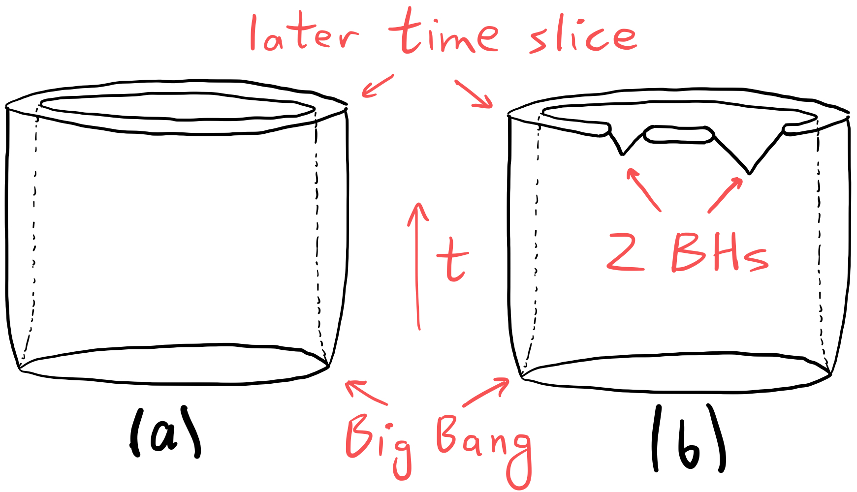
vi) This CPT-symmetric picture for black mirrors fits naturally in the CPT-symmetric picture of the cosmos advocated in Boyle et al. (2018, 2022a); Boyle and Turok (2021a, b); Boyle et al. (2022b); Turok and Boyle (2024); Boyle and Turok (2024); Turok and Boyle (2023) (see Fig. 6): the two sheets of spacetime split at the Bang, and merge at BHs. As before, it is natural to regard the two-sheeted spacetime as representing a pure state, while one sheet represents the mixed state obtained by tracing over the other sheet. This neatly explains why the corresponding entropy, associated with the boundary surface separating the two sheets, is given by the horizon area (in the BH case) Bekenstein (1972, 1973); Gibbons and Hawking (1977), and the total comoving spatial volume (in the cosmological case Turok and Boyle (2024); Boyle and Turok (2024)).
Acknowledgements.
KT wishes to thank Mihalis Dafermos and Matt Visser for their helpful comments during the Strong Gravity conference. LB is grateful to Minhyong Kim for helpful discussions. KT, LB, and NT are supported by the STFC Consolidated Grant ‘Particle Physics at the Higgs Centre’, and NT is supported by the Higgs Chair at the University of Edinburgh. Research at Perimeter Institute is supported by the Government of Canada, through Innovation, Science and Economic Development, Canada and by the Province of Ontario through the Ministry of Research, Innovation and Science.References
- Einstein and Rosen (1935) Albert Einstein and N. Rosen, “The Particle Problem in the General Theory of Relativity,” Phys. Rev. 48, 73–77 (1935).
- Oppenheimer and Snyder (1939) J. R. Oppenheimer and H. Snyder, “On continued gravitational contraction,” Phys. Rev. 56, 455–459 (1939).
- Dafermos and Luk (2017) Mihalis Dafermos and Jonathan Luk, “The interior of dynamical vacuum black holes I: The -stability of the Kerr Cauchy horizon,” (2017), arXiv:1710.01722 [gr-qc] .
- Hawking (1976) S. W. Hawking, “Breakdown of Predictability in Gravitational Collapse,” Phys. Rev. D 14, 2460–2473 (1976).
- Almheiri et al. (2013) Ahmed Almheiri, Donald Marolf, Joseph Polchinski, and James Sully, “Black Holes: Complementarity or Firewalls?” JHEP 02, 062 (2013), arXiv:1207.3123 [hep-th] .
- Gibbons (1986) G. W. Gibbons, “The elliptic interpretation of black holes and quantum mechanics,” Nucl. Phys. B 271, 497–508 (1986).
- Saravani et al. (2015) Mehdi Saravani, Niayesh Afshordi, and Robert B. Mann, “Empty black holes, firewalls, and the origin of Bekenstein–Hawking entropy,” Int. J. Mod. Phys. D 23, 1443007 (2015), arXiv:1212.4176 [hep-th] .
- Visser (1989a) Matt Visser, “Traversable wormholes: Some simple examples,” Phys. Rev. D 39, 3182–3184 (1989a), arXiv:0809.0907 [gr-qc] .
- Visser (1989b) Matt Visser, “Traversable wormholes from surgically modified Schwarzschild space-times,” Nucl. Phys. B 328, 203–212 (1989b), arXiv:0809.0927 [gr-qc] .
- ’t Hooft (2016) Gerard ’t Hooft, “Black hole unitarity and antipodal entanglement,” Found. Phys. 46, 1185–1198 (2016), arXiv:1601.03447 [gr-qc] .
- ’t Hooft (2017) Gerard ’t Hooft, “The Firewall Transformation for Black Holes and Some of Its Implications,” Found. Phys. 47, 1503–1542 (2017), arXiv:1612.08640 [gr-qc] .
- d’Invemo (1992) Ray d’Invemo, Introducing Einstein’s relativity (Oxford University Press, 1992).
- Gibbons and Hawking (1977) G. W. Gibbons and S. W. Hawking, “Action Integrals and Partition Functions in Quantum Gravity,” Phys. Rev. D 15, 2752–2756 (1977).
- York (1972) James W. York, Jr., “Role of conformal three geometry in the dynamics of gravitation,” Phys. Rev. Lett. 28, 1082–1085 (1972).
- Gibbons et al. (2004) G. W. Gibbons, H. Lu, Don N. Page, and C. N. Pope, “Rotating black holes in higher dimensions with a cosmological constant,” Phys. Rev. Lett. 93, 171102 (2004), arXiv:hep-th/0409155 .
- Gibbons et al. (2005) G. W. Gibbons, H. Lu, Don N. Page, and C. N. Pope, “The General Kerr-de Sitter metrics in all dimensions,” J. Geom. Phys. 53, 49–73 (2005), arXiv:hep-th/0404008 .
- Hollands et al. (2024) Stefan Hollands, Robert M. Wald, and Victor G. Zhang, “Entropy of dynamical black holes,” Phys. Rev. D 110, 024070 (2024), arXiv:2402.00818 [hep-th] .
- Vachaspati et al. (2007) Tanmay Vachaspati, Dejan Stojkovic, and Lawrence M. Krauss, “Observation of incipient black holes and the information loss problem,” Phys. Rev. D 76, 024005 (2007), arXiv:gr-qc/0609024 .
- Vachaspati and Stojkovic (2008) Tanmay Vachaspati and Dejan Stojkovic, “Quantum radiation from quantum gravitational collapse,” Phys. Lett. B 663, 107–110 (2008), arXiv:gr-qc/0701096 .
- Kawai et al. (2013) Hikaru Kawai, Yoshinori Matsuo, and Yuki Yokokura, “A Self-consistent Model of the Black Hole Evaporation,” Int. J. Mod. Phys. A 28, 1350050 (2013), arXiv:1302.4733 [hep-th] .
- Sewell (1982) Geoffrey L. Sewell, “Quantum fields on manifolds: PCT and gravitationally induced thermal states,” Annals Phys. 141, 201–224 (1982).
- Hawking (2014) S. W. Hawking, “Information Preservation and Weather Forecasting for Black Holes,” (2014), arXiv:1401.5761 [hep-th] .
- Hawking (1975) S. W. Hawking, “Particle Creation by Black Holes,” Commun. Math. Phys. 43, 199–220 (1975), [Erratum: Commun.Math.Phys. 46, 206 (1976)].
- Witten (2018) Edward Witten, “Symmetry and Emergence,” Nature Phys. 14, 116–119 (2018), arXiv:1710.01791 [hep-th] .
- Harlow and Ooguri (2019) Daniel Harlow and Hirosi Ooguri, “Constraints on Symmetries from Holography,” Phys. Rev. Lett. 122, 191601 (2019), arXiv:1810.05337 [hep-th] .
- Harlow and Ooguri (2021) Daniel Harlow and Hirosi Ooguri, “Symmetries in quantum field theory and quantum gravity,” Commun. Math. Phys. 383, 1669–1804 (2021), arXiv:1810.05338 [hep-th] .
- Boyle et al. (2018) Latham Boyle, Kieran Finn, and Neil Turok, “CPT-Symmetric Universe,” Phys. Rev. Lett. 121, 251301 (2018), arXiv:1803.08928 [hep-ph] .
- Boyle et al. (2022a) Latham Boyle, Kieran Finn, and Neil Turok, “The Big Bang, CPT, and neutrino dark matter,” Annals Phys. 438, 168767 (2022a), arXiv:1803.08930 [hep-ph] .
- Boyle and Turok (2021a) Latham Boyle and Neil Turok, “Two-Sheeted Universe, Analyticity and the Arrow of Time,” (2021a), arXiv:2109.06204 [hep-th] .
- Boyle and Turok (2021b) Latham Boyle and Neil Turok, “Cancelling the vacuum energy and Weyl anomaly in the standard model with dimension-zero scalar fields,” (2021b), arXiv:2110.06258 [hep-th] .
- Boyle et al. (2022b) Latham Boyle, Martin Teuscher, and Neil Turok, “The Big Bang as a Mirror: a Solution of the Strong CP Problem,” (2022b), arXiv:2208.10396 [hep-ph] .
- Turok and Boyle (2024) Neil Turok and Latham Boyle, “Gravitational entropy and the flatness, homogeneity and isotropy puzzles,” Phys. Lett. B 849, 138443 (2024), arXiv:2201.07279 [hep-th] .
- Boyle and Turok (2024) Latham Boyle and Neil Turok, “Thermodynamic solution of the homogeneity, isotropy and flatness puzzles (and a clue to the cosmological constant),” Phys. Lett. B 849, 138442 (2024), arXiv:2210.01142 [gr-qc] .
- Turok and Boyle (2023) Neil Turok and Latham Boyle, “A Minimal Explanation of the Primordial Cosmological Perturbations,” (2023), arXiv:2302.00344 [hep-ph] .
- Bekenstein (1972) J. D. Bekenstein, “Black holes and the second law,” Lett. Nuovo Cim. 4, 737–740 (1972).
- Bekenstein (1973) Jacob D. Bekenstein, “Black holes and entropy,” Phys. Rev. D 7, 2333–2346 (1973).
- Carter (1968) B. Carter, “Hamilton-Jacobi and Schrodinger separable solutions of Einstein’s equations,” Commun. Math. Phys. 10, 280–310 (1968).
- Carter (1973) B. Carter, “Black holes equilibrium states,” in Les Houches Summer School of Theoretical Physics: Black Holes (1973) pp. 57–214.
- Plebanski and Demianski (1976) J. F. Plebanski and M. Demianski, “Rotating, charged, and uniformly accelerating mass in general relativity,” Annals Phys. 98, 98–127 (1976).
- Caldarelli et al. (2000) Marco M. Caldarelli, Guido Cognola, and Dietmar Klemm, “Thermodynamics of Kerr-Newman-AdS black holes and conformal field theories,” Class. Quant. Grav. 17, 399–420 (2000), arXiv:hep-th/9908022 .
- Coleman (1985) Sidney Coleman, Aspects of Symmetry: Selected Erice Lectures (Cambridge University Press, Cambridge, U.K., 1985).
- Stueckelberg (1941a) E. C. G. Stueckelberg, “La signification du temps propre en mécanique ondulatoire,” Helvetica physica acta 14, 322–323 (1941a).
- Stueckelberg (1941b) Ernst Carl Gerlach Stueckelberg Stueckelberg, “Un nouveau modele de l’électron ponctuel en théorie classique,” Helv. Phys. Acta 14, 51–80 (1941b).
- Stueckelberg (1941c) E. C. G. Stueckelberg, “Remarks on the creation of pairs of particles in the theory of relativity,” Helv. Phys. Acta 14, 588–594 (1941c).
Appendix A General Stationary Black Mirror
A.1 Boyer-Lindquist coordinates
Consider the general charged, rotating black hole exterior in dS or AdS Carter (1968, 1973); Plebanski and Demianski (1976); Caldarelli et al. (2000). We start in generalized Boyer-Lindquist coordinates – the generalization of the Schwarzschild coordinates considered Section II. We define the tetrad
| (9a) | |||||
| (9b) | |||||
| (9c) | |||||
| (9d) | |||||
where we have defined
| (10) |
with the rotation parameter, the AdS radius, and , with and the electric and magnetic charges, respectively. (To obtain the corresponding dS black hole, just make the substitution .) Then the line element is
| (11a) | |||||
| and the electromagnetic potential and field strength are given by | |||||
| (11b) | |||||
| and | |||||
| (11c) | |||||
Note that if , where is defined in Eq. (8) in Caldarelli, Cognola and Klemm (1999), then the black hole is super-extremal; has no real roots and hence no horizons, and a naked singularity. We will henceforth assume the opposite, that , so that the black hole is sub-extremal, with two real roots, and . The BH horizon is located at the outer root , and the horizon area is given by
| (12) |
Boyer-Lindquist coordinates make manifest the full symmetry of the exterior spacetime: two Killing vectors and , and two discrete symmetries which send to, respectively, and .
A.2 Going Euclidean, thermodynamics
To construct the Euclidean metric, we start with Boyer-Lindquist coordinates , and make the Wick rotations , , , and consider real values of , , and , thus obtaining the new tetrad
| (13a) | |||||
| (13b) | |||||
| (13c) | |||||
| (13d) | |||||
where
| (14) |
Then the Euclidean line element is
| (15) |
Next we switch radial coordinate , by making the substitution
| (16) |
where is the Wick rotation of the previous horizon radius (and a root of ), the constant is determined below. Then, to leading order in , the metric becomes
| (17) |
where
| (18a) | |||||
| (18b) | |||||
and we see that, by choosing we can set the leading coefficient in (17) to unity.
As in the Schwarzschild case, we see the Euclidean metric has the topology of a one-sided 2-cone (parameterized by , , with its tip at ) times a 2-sphere (parameterized by , ) – i.e. the blue side of Fig. 2a. And, as before, we can analytically extend this to a 2-sided cone by letting extend to negative values (the blue+red surface in Fig. 2a). Note that this extended metric now has a new isometry .
In order to make the metric smooth at the cone’s tip (to remove the conic singularity, as in Fig. 2b), we must identify ; and, in since this identification must be -independent, we are forced to identify
| (19) |
where
| (20a) | |||||
| (20b) | |||||
Note that this same shift leaves invariant.
Now, Wick-rotating back to Lorentzian signature, and expressing everything in terms of our original Lorentzian variables, we have the identification
| (21) |
where
| (22a) | |||||
| (22b) | |||||
Here is identified as the temperature of the black hole, and as the angular velocity of the horizon.
A.3 In Eddington-Finkelstein coordinates
Although the Boyer-Lindquist system has the advantage that it makes manifest the full symmetry of the metric, it has the disadvantage that it only covers the exterior , and fails to extend to (or beyond) the black and white horizons (where it becomes singular). To fix this, we first define new generalized ingoing/outgoing Eddington-Finkelstein coordinates that remain non-singular on one horizon or the other, by a coordinate transformation of the form
| (23a) | |||||
| (23b) | |||||
where and are chosen to make the term drop out of the line element in the new (Eddington-Finkelstein) coordinate system. One can check that this implies
| (24a) | |||||
| (24b) | |||||
where the sign corresponds to ingoing/outgoing Eddington-Finkelstein coordinates which cover the exterior and black/white horizon, respectively.
In these new coordinates, if we define the new tetrad
| (25a) | |||||
| (25b) | |||||
| (25c) | |||||
| (25d) | |||||
the line element is
| (26e) | |||||
| the gauge potential is | |||||
| (26f) | |||||
| (where we removed an additional term via a gauge transformation), and the field strength is | |||||
| (26g) | |||||
We see that these coordinates remain non-singular at the black/white horizon (where vanishes): the components of , and all remain finite, and the metric determinant remains finite and non-zero.
Now, as before, we can switch from by making the substitution (16) in Eqs. (25, 26, 26f, 26g) and extending to negative values. If we now let the coordinates and (respectively, and ) extend from to , we obtain the general stationary black mirror, described in ingoing coordinates (respectively, outgoing coordinates ) which cover the entire spacetime except for the black horizon (respectively, white horizon). Taken together, these ingoing and outgoing coordinate systems provide an atlas covering the complete stationary black mirror spacetime.
As before, the extended spacetime now has a new isometry that takes us back and forth between the two exterior regions ( and ’), which are identified at the horizon, as in Fig. 1b.
Note that, in these coordinates, the components of the resulting metric and field strength , as well as the components of all curvature invariants (such as the Kretschmann scalar ) are again everywhere explicitly smooth, analytic and finite, so the spacetime has no curvature singularities. But, as in the Schwarzschild case, two of the eigenvalues of the metric are exchanged as we cross the horizon, , and both of these eigenvalues have simple analytic zeros at , while the corresponding eigenvalues of have simple poles).
Appendix B Saddle points of the action
In this appendix, we show that the Schwarzchild black mirror presented in Section II is a regular saddle of the Einstein-Hilbert action
| (27) |
The boundary terms are needed to ensure that the variation of the action yields the Einstein equations when the metric is held fixed on the boundary, with no constraint on its normal derivative there. The Einstein-Hilbert action does not have this property because it involves second derivatives of the metric. However, it can be reduced to an action involving only first derivatives by performing integrations by parts and discarding the boundary terms. The corrected action is then the appropriate one for a quantum path integral between an initial and a final three-geometry.
A general principle, discussed by Coleman Coleman (1985), states that if an action respects a symmetry then saddles of the action restricted to configurations which respect are also saddles of the full action. Hence, saddles of the gravitational action restricted to spherically symmetric spacetimes are also saddles of the full gravitational action. Consider the most general spherically symmetric line element,
| (28) |
Here, and are -invariant coordinates. We do not assume the metric is static and include an arbitrary “shift” as well as a “lapse” function . One can use the residual coordinate freedom to set equal to zero and to choose as the radial coordinate. However, is not a good coordinate for our analytically extended spacetime and it is better to regard it as a function of a coordinate which is.
In order to recover the full set of Einstein equations governing such metrics, one must vary the gravitational action before further restricting the coordinates. As we shall see, varying the action with respect to the shift yields a constraint that the lapse depends only on . (This is the crux of Birkhoff’s theorem, that every spherically symmetric solution of the Einstein equations is static.) Similarly, varying the action with respect to yields a constraint on and and their first derivatives. After obtaining these constraints, we can redefine the time coordinate to eliminate and reparameterize to set to unity. Finally, by varying the action with respect to and we obtain the second order field equations. These imply that has a trivial time dependence which can be removed by reparameterizing .
To calculate the action (27) restricted to spherical symmetric spacetimes, we insert the ansatz (28) into the Einstein-Hilbert term and integrate by parts to eliminate second derivatives. We need only retain terms of first order in since it is set to zero after calculating the first order variations. After several integrations by parts, the action reduces (up to terms of higher order in ) to
| (29) |
where dot denotes and prime . Note a crucial subtlety: that in deriving this expression, we have used the positive square root of in the volume form, and we have also taken the orientation on the 2-sphere to as we pass from to : see Appendix C. Setting the variation with respect to zero yields the constraint that . (As will be seen later, in the solution is finite and non-vanishing everywhere.) Varying the action with respect to and then setting it to unity yields the constraint
| (30) |
Varying the action with respect to and then yields the two second order field equations
| (31a) | |||||
| (31b) | |||||
Eq. (31a) is solved by noticing that is constant, so that with a constant. This implies . Now (30) yields which is integrated to obtain with an arbitrary function. Assuming it is nonzero, it can be set to unity by redefining the time coordinate via .
We now impose CPT symmetric boundary conditions. As we shall explain momentarily, will imply that is an odd function of . To find the solutions explicitly, we set
| (32) |
The solution is then , so that, in the coordinate system, the line element is
| (33) |
with . The time-like one-form of the tetrad is odd in and has a simple zero at , whereas the space-like one-forms are even and nonzero throughout. The spatial metric is conformal to a cylinder , of radius . In the near-horizon limit () the coordinate where is the proper radial coordinate used in Eqs. (4–7); whereas far from the horizon () the line element (33) becomes which, with , is just Minkowski spacetime.
Note that, the total action (29) – which is the sum of the Einstein-Hilbert bulk action and the Gibbons-Hawking-York boundary terms – vanishes when we integrate over a symmetric range from to , because the integrand is an odd function of .
The method used here can be straightforwardly generalized to spherically symmetric electro-vacuum solutions that are asymptotically flat, de Sitter or anti-de Sitter. This time, after using various equations of motion obtained from the action, the line element takes the form
| (34) |
with
| (35a) | |||||
| (35b) | |||||
The function has at most four roots: which corresponds to the Cauchy horizon, which corresponds to the event horizon and which corresponds to the cosmological horizon, with if . Since it follows that the range of lies in the interval . Moreover, CPT symmetry implies that obeys , and therefore is a root of . If then the function is a constant. Thus, the only physical initial conditions for are and . Extending this solution to the horizon by changing coordinates from Schwarzschild time to Eddington-Finkelstein time ( or ) once again brings us back to the black mirror geometry discussed in the main text.
Appendix C CPT symmetry
In the body of the paper, we focused for simplicity on the Schwarzschild (static, uncharged) black mirror, but let us now consider the general stationary black mirror (including charge), to understand the action of CPT symmetry more clearly. For simplicity, assume the mirror has electric charge but no magnetic charge.
The natural CPT transformation Sewell (1982) maps a point with coordinates or, equivalently, . This is an isometry that leaves both the line element , as well as the field strength invariant. However, due to the inversion of the orientation of the two-sphere, the net charge calculated via Gauss’s law from the net flux through this two sphere changes sign under this transformation. In this sense, it not only inverts spacetime, but also reverses electric charges, and is thus a CPT transformation.
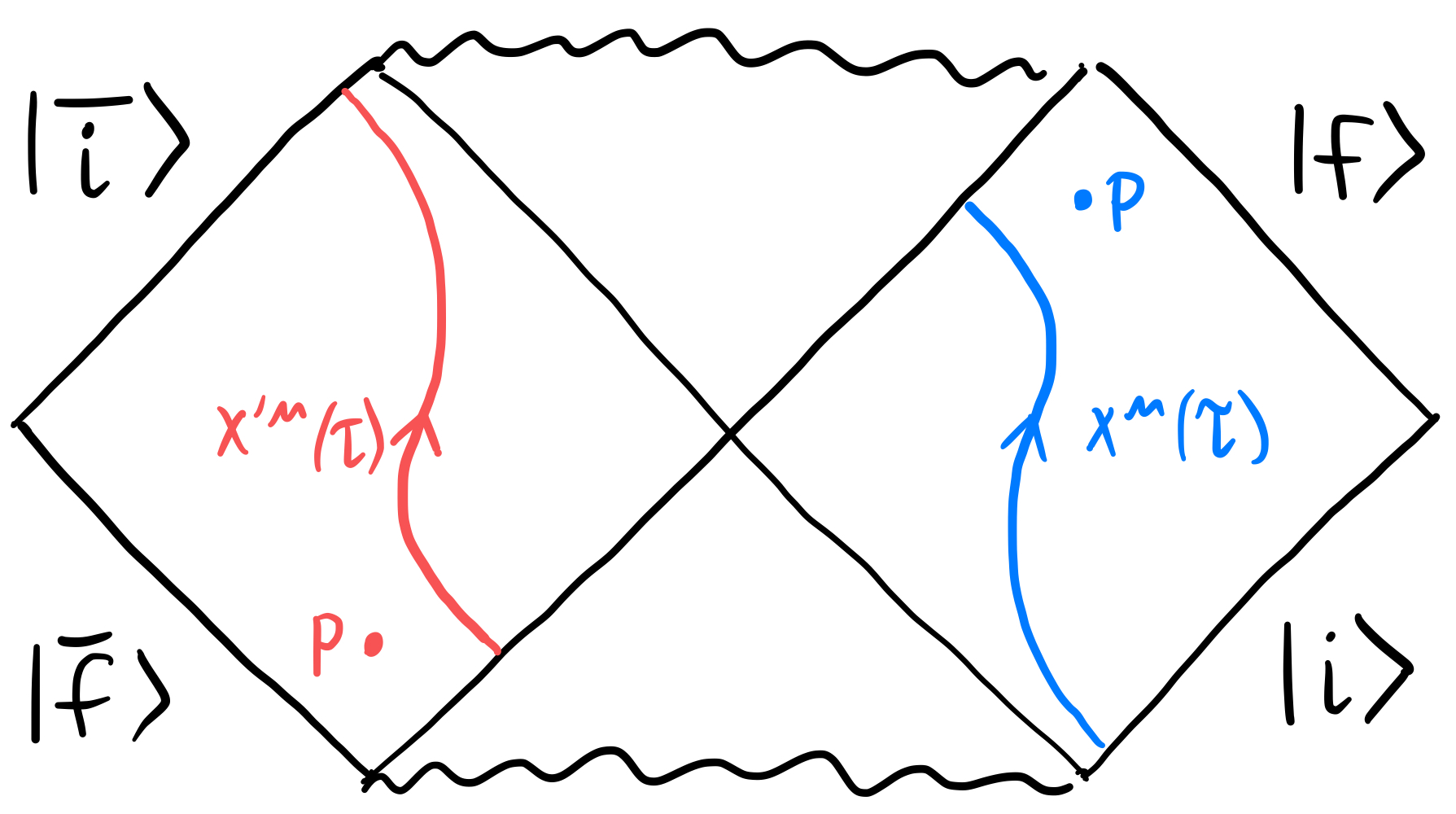
This isometry maps e.g. a point with angular coordinate near the upper corner of exterior to a mirror point near with angular coordinate near the lower corner of exterior (see Fig. 5).
The trajectory of particle of charge in the black mirror spacetime, satisfies the equation of motion
| (36) |
where a dot denotes a proper time derivative . Performing a transformation on the background also maps the trajectory to a new trajectory , see Fig. 5. Moreover, since this map reverses the orientation on the 2-spheres, it not only reverses the charge of the black hole (as measured by Gauss’s law using a sphere surrounding the hole), it also reverses the charge of the point particle (again as measured by Gauss’s law using a sphere surrounding the point charge). This is why, in Figs. 3,4, and 5, the arrows showing charge flow (more correctly, the direction of ) in the left-hand (red) trajectories are reversed relative to the corresponding arrows on the right-hand (blue) trajectories.333This insight, that an antiparticle is just a particle moving backward in time – i.e. a particle whose “worldline time” (proper time) has been reversed relative to the ”embedding time” (the time direction in the target space) is due to Stueckelberg Stueckelberg (1941a, b, c).