Assessing the Role of Volumetric Brain Information in Multiple Sclerosis Progression

Abstract

Multiple sclerosis is a chronic autoimmune disease that affects the central nervous system. Understanding multiple sclerosis progression and identifying the implicated brain structures is crucial for personalized treatment decisions. Deformation-based morphometry utilizes anatomical magnetic resonance imaging to quantitatively assess volumetric brain changes at the voxel level, providing insight into how each brain region contributes to clinical progression with regards to neurodegeneration. Utilizing such voxel-level data from a relapsing multiple sclerosis clinical trial, we extend a model-agnostic feature importance metric to identify a robust and predictive feature set that corresponds to clinical progression. These features correspond to brain regions that are clinically meaningful in MS disease research, demonstrating their scientific relevance. When used to predict progression using classical survival models and 3D convolutional neural networks, the identified regions led to the best-performing models, demonstrating their prognostic strength. We also find that these features generalize well to other definitions of clinical progression and can compensate for the omission of highly prognostic clinical features, underscoring the predictive power and clinical relevance of deformation-based morphometry as a regional identification tool.

Keywords: multiple sclerosis; deformation-based morphometry; survival analysis; feature selection; random forest; convolutional neural network

1 Introduction

Multiple sclerosis (MS) is a chronic autoimmune disease that affects the central nervous system (CNS) in young adults (Compston and Coles,, 2008). Magnetic resonance imaging (MRI) of the brain is a key tool for diagnosing and monitoring MS progression. Different types of MRI data possess overlapping yet complementary properties and applications. For instance, brain volume measurements derived from T1-weighted MRI provide insights into brain atrophy, which is associated with disability and disease progression (Chard et al.,, 2002; Bermel and Bakshi,, 2006; Lomer et al.,, 2024; Fisniku et al.,, 2008). Deformation-based morphometry (DBM), an image registration-based method (Ashburner et al.,, 1998; Chung et al.,, 2001), provides voxel-level measurements of volume differences across the entire brain which offers finer-grained insights into spatially distributed neurodegeneration (Azevedo et al.,, 2018; Rocca et al.,, 2021). MRI data has proven instrumental in predicting disease progression and plays a critical role in personalizing patient treatment decisions (Rocca et al.,, 2019). Additionally, identifying specific brain regions with volume changes linked to disease progression enhances patient monitoring and facilitates the evaluation of treatment efficacy (Song et al.,, 2022).

Despite recent progress in using T1-weighted MRI data to predict MS progression (Moazami et al.,, 2021; Vázquez-Marrufo et al.,, 2022; Lomer et al.,, 2024; Prathapan et al.,, 2024), several open questions remain regarding how data and methodological choices may affect model reliability. For example, recent work leveraging random survival forests achieved high accuracy in predicting clinical progression over a 10-year period based on changes in T1-weighted MRI-derived features within the first 2 years (Pisani et al.,, 2021). However, baseline T1-weighted MRI data alone demonstrated relatively limited predictive power for 2-year progression (Pellegrini et al.,, 2020). Similarly, it was shown that, while voxel clusters derived from independent components analysis (ICA) applied to 2-year volume change data were predictive of 10-year progression, the voxel cluster values at baseline were similar between progressors and non-progressors (Bergsland et al.,, 2018). Some studies have also noted unclear predictive value of T1-weighted MRI, which can vary between studies and can depend on outcome definitions (Pellegrini et al.,, 2020; Tousignant et al.,, 2019). These issues also persist in deep learning frameworks (Zhang et al.,, 2023; Coll et al.,, 2024). It also remains unclear whether T1-weighted MRI data provides complementary information for progression prediction beyond clinician-measured variables of disease state, some of which are used to define common progression endpoints themselves (Sormani et al.,, 2010; Cadavid et al.,, 2017). Ultimately, there is a lack of literature on detecting baseline volume measurements from T1-weighted brain MRI that are predictive of clinical progression within two years. For broader reviews of data-driven approaches to clinical modeling of MS, we refer readers to Moazami et al., (2021); Vázquez-Marrufo et al., (2022); Lomer et al., (2024); Prathapan et al., (2024).

In this study, we utilize deformation-based morphometry derived from T1-weighted MRI of a Phase III MS clinical trial (Hauser et al.,, 2017; Song et al.,, 2022) to investigate the impact of various methodological choices, particularly those used to identify predictive DBM features, on the reliability of conclusions drawn from this dataset. We first employ a state-of-the-art, model-agnostic feature importance algorithm, adapted using leave-one-covariate-out methods (Lei and Wasserman,, 2014) and minipatch ensembles (LOCO-MP) (Gan et al.,, 2023), to identify brain regions from low-signal T1-weighted MRI baseline data that are predictive of MS progression. While general feature importance metrics can be applied, they often yield inconsistent results when the data are highly correlated and high-dimensional (Agarwal et al.,, 2023). LOCO-MP leverages learning from small feature subsets to isolate the effects of highly correlated regions. When applied to region-based summary statistics of volumetric T1-weighted MRI data, this method identifies regions implicated in MS progression, outperforming standard feature importance approaches.

Next, we apply traditional survival models to examine how different outcome/endpoint definitions, in conjunction with feature selection by LOCO-MP, influence prediction power. Although our progression endpoint (CCDP24, discussed in Section 2.1) is highly censored within the two-year study period, it represents a well-defined and clinically meaningful composite marker of MS progression. To validate the DBM features identified using LOCO-MP, we assess their generalizability across alternative progression endpoints (S25FW, discussed in Section 2.1). This also allows us to compare a single, objective measure of physical disability with the composite measure, the latter involving some degree of clinician discretion (Sormani et al.,, 2010). By using DBM at baseline to identify patient volumetric abnormalities and by applying LOCO-MP to enforce sparsity in the DBM feature set, we achieve improved prediction performance compared to models that use whole-brain T1-weighted MRI data as input. Interestingly, models using selected MRI features alone perform on par with those based solely on conventional (non-DBM) measurements. Combined models incorporating both selected MRI features and conventional measures do not necessarily outperform individual models (those using either selected MRI features or conventional measures alone). Notably, removing baseline conventional variables that define certain endpoints significantly reduces the predictive power of the conventional feature models, underscoring the strong predictive value of the selected MRI features.

We further analyze whether 3D convolutional neural networks (CNNs) using only the LOCO-MP regions perform better than full brain architectures. We develop a 3D CNN architecture, Region CNN, that accepts a set of atlas region tensors as input. While full brain MRI deep transformer models (Dai et al.,, 2021; Yu et al.,, 2023) are unstable and show low prediction accuracy, Region CNN using LOCO-MP identified features performs substantially better. This highlights the importance in filtering out unnecessary regions via LOCO-MP for extracting prognostic signal from CNNs for this cohort.

2 Materials and methods

2.1 Data and image preprocessing

The data used in this study are from a comparator arm of a phase 3 clinical trial of relapsing multiple sclerosis (OPERA I: NCT01247324), in which the patients were treated with interferon (IFN) $\beta$-1a (44 $\mu$g) three times per week throughout the 96-week treatment period. Our sample consisted of 350 patients. Details on patient selection, MRI acquisition, and clinical assessments are provided in the original report (Hauser et al.,, 2017). Briefly, patients were recruited with an age range of 18 to 55 years; McDonald criteria diagnosis of multiple sclerosis; Expanded Disability Status Scale (EDSS) score between 0 to 5.5; more than 2 documented clinical relapses within the previous 2 years or one clinical relapse within the year before screening; brain MRI evidence of multiple-sclerosis-related abnormalities. Conventional T1-weighted 3D spoiled gradient-recalled echo brain MRI was acquired at baseline, Weeks 24, 48 and 96 (repetition time = 28–30 ms, echo time = 5–11 ms, flip angle = 27–30 deg, 60 oblique axial slices of 1 mm in-plane resolution and 3 mm slice thickness). The primary clinical outcome was defined as a composite measure of disability progression which included three clinical assessments: EDSS, Timed 25-Foot Walk (T25FW, a measure of short distance walking speed), and 9-Hole Peg Test (9HPT, a measure of upper limb function) (Elliott et al.,, 2019). This composite measure was developed to capture a broader aspect of disability in patients with multiple sclerosis. The 24-week composite confirmed disability progression (CCDP24) was defined as progression on any one of the three components (EDSS, T25FW, or 9HPT): an increase of EDSS score from the baseline at least 1.0 point (or 0.5 points if the baseline EDSS score was larger than 5.5) or a 20% minimum threshold change for T25FW and 9HPT. We also consider a 24-week progression outcome based solely on the 25-foot walking score (S25FW) in Section 3.2.2. Table 1 summarizes the data in terms of dimension and number of relevant features.

Since MS progression is influenced by many factors, our models consider a variety of baseline demographic and clinical measurements as well as standard imaging metrics. Broadly speaking, we refer to these features as “conventional features” to distinguish them from DBM-based features. The conventional features serve as a comparison against the DBM features to assess which feature set performs more optimally. We record nine conventional features which include the patient’s age, birth sex, years of onset, weight (in kg), total brain volume, total T2 lesion volume, baseline 25-foot walking test score, baseline 9-hole peg test score, and baseline EDSS, which are generally thought to be related to MS disease progression (Bar-Or et al.,, 2023).

Sample size	# conventional features	# DBM regions	Summary features	Outcomes
350	9	51	Median, St. Dev	CCDP24, S25FW

Table 1: OPERA I data summary.

Statistical features of regional brain volume were extracted from T1-weighted brain MRI, using a deformation-based morphometry (DBM) pipeline based on the diffeomorphic image registration of advanced normalization tools (Tustison et al.,, 2019).

Figure 1: Illustration of the deformation-based morphometry (DBM) analysis. For each T1-weighted brain MR image, the registration with the group template generates a Jacobian map over the whole brain, which is a voxel-level measure of volume relative to the group template. Regional labels on the brain atlas were mapped to the group template to extract statistical features of the Jacobian maps at the patient level.

The Mindboggle atlas was used to identify individual brain regions (Klein et al.,, 2017). In addition, prior probability images of six major brain regions based on the Mindboggle atlas, including CSF, cortical grey matter, deep grey matter, cortical white matter, the brainstem, and the cerebellum, were binarized at a probability threshold of 0.5. A population-specific group template of the T1-weighted brain MRI was constructed by advanced normalization tools with T1-weighted brain MRI images of 171 healthy adults (aged 20–59 years). Before being fed into the pipeline, each individual brain image was preprocessed with the following steps: 1) resampling to an isotropic resolution of 1 mm; 2) N4 bias correction (Tustison et al.,, 2010); and 3) denoising with a non-local algorithm (Manjón et al.,, 2010). Regional labels were mapped from the group template to individual images so that volume change of any predefined region could be measured.

The tabular DBM feature set consists of the median and standard deviation voxel values for each of the 51 atlas regions, resulting in 102 total features. Prior to performing feature selection and modeling, we filter out features with a variance below 0.01 across all patients, reducing the number of DBM features from 102 to 56. No other conventional features were excluded in this filtering step.

2.2 Feature importance using minipatch ensembles

In high dimensional data sets, variable importance metrics are commonly used to filter out variables that are inconsequential to prediction and retain those with the most predictive value. For random forest models, feature importance is typically summarized by averaging the “out-of-bag” prediction error across trees when that feature is permuted (Ishwaran and Kogalur,, 2019; Breiman et al.,, 2018). However, these metrics may produce misleading results, especially when correlated features are present (Agarwal et al.,, 2023). As such, to identify the most important DBM features and brain regions associated with MS progression, we extend a feature importance method called leave-one-covariate-out minipatch (LOCO-MP) prediction (Lei and Wasserman,, 2014; Yao and Allen,, 2021; Gan and Allen,, 2022; Gan et al.,, 2023) to survival analysis. Our outcome of interest, patient progression, is recorded as a time-to-event pair $(T_{i},C_{i})$, where $T_{i}$ is the event time and $C_{i}\in\left\{0,1\right\}$ is an indicator for whether the patient experiences progression ($C_{i}=1$) or is censored for whatever reason ($C_{i}=0$). LOCO-MP determines feature importance for a certain target feature by aggregating predictions across multiple data subsamples (called “minipatches”) and comparing the average prediction performance across minipatches with and without that feature. Dependencies between features are addressed through aggregating the minipatches, which ensures that each feature’s predictive value is not overshadowed by other correlated features. The procedure is summarized graphically in Figure 2 and outlined below for a target feature $j$:

1. Subsample the data: Subsample a set of observations (rows) and features (columns), denoted by purple cells. This forms a “minipatch.”

2. Train a model: Fit a model to the minipatch and evaluate predictions using the remaining observations (blue cells).

3. Repeat steps 1 and 2 over multiple minipatches.

4. Compute feature importance: Compute $\bar{\Delta}_{j}$, the feature importance score of feature $j$ (discussed in the following paragraphs).

Because our outcomes of interest are recorded in a time-to-event format, we extend LOCO-MP to survival analysis by utilizing discrete hazard loss functions to assess individual-level error, as discussed further below.

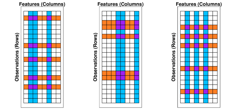
Figure 2: General overview of LOCO-MP. Each plot demonstrates how a subset of observations (orange) and features (blue) are subsampled to form a “minipatch” (purple cells). A model is trained on the purple cells and predictions are generated using the unselected observations (blue cells). This process is repeated over numerous minipatches to ensure each feature and observation is selected enough times to perform inference. Feature importance for a target feature is assessed by evaluating performance on minipatches with and without that feature.

Details of LOCO-MP for survival analysis

Following the notation of Gan et al., (2023), we denote the $N\times M$ data matrix as $X$ and the outcome as $Y$. Let $(X_{i},Y_{i})$ denote the feature-outcome pair for individual $i$, where $X_{i}$ is a $M$-dimensional vector and $Y_{i}=(T_{i},C_{i})$. For every minipatch $k=1\dots K$, we sample $n$ observations $I_{k}$ and $m$ features $F_{k}$ from $X$. Denote this minipatch as $X_{I_{k},F_{k}}$. A prediction model $\hat{\mu}_{k}$ is then trained on $X_{I_{k},F_{k}}$ and predictions are generated for the remaining observations $X_{{-I_{k},F_{k}}}$, which includes features $F_{k}$ and observations outside $I_{k}$. Repeating this over all $K$ minipatches, we compute the individual feature occlusion score for feature $j$ and observation $i$:

$$\hat{\Delta}_{ij}=\text{Error}(Y_{i},\hat{\mu}_{-i}^{-j}(X_{i}))-\text{Error}\left(Y_{i},\hat{\mu}_{-i}(X_{i})\right),$$

where

$$\hat{\mu}_{-i}(X_{i}) =\frac{1}{\sum_{k=1}^{K}\mathbbm{1}(i\notin I_{k})}\sum_{k=1}^{K}\mathbbm{1}(i\notin I_{k})\hat{\mu}_{k}(X_{i}),\text{ and}$$

$$\hat{\mu}_{-i}^{-j}(X_{i}) =\frac{1}{\sum_{k=1}^{K}\mathbbm{1}(i\notin I_{k})\mathbbm{1}(j\notin F_{k})}\sum_{k=1}^{K}\mathbbm{1}(i\notin I_{k})\mathbbm{1}(j\notin F_{k})\hat{\mu}_{k}(X_{i}),$$

and $\text{Error}()$ refers to any observation-level prediction error function, in our case the discrete hazard loss discussed in the following paragraph. The individual $\hat{\Delta}_{ij}$ values are then averaged, giving us the feature occlusion score for feature $j$:

$$\bar{\Delta}_{j}=\frac{1}{N}\sum_{i=1}^{N}\hat{\Delta}_{ij}.$$ (1)

$\hat{\Delta}_{ij}$ is the difference in error for observation $i$ when feature $j$ is omitted. Concretely, this can be thought of as the change in prediction capability for patient $i$ when a specific DBM feature is omitted. Larger, positive values of $\hat{\Delta}_{ij}$ indicate greater feature importance since the model performs worse (has larger error) when feature $j$ is excluded.

The prediction error for survival analysis models is commonly measured as the reciprocal of the overall concordance index (C-index) of risk scores between pairs of observations. However, this metric is not an aggregation of observation-level errors, preventing its direct usage in the LOCO-MP framework. To address this, we utilize discrete hazard loss functions used in deep learning survival analysis models (Zadeh and Schmid,, 2020; Vale-Silva and Rohr,, 2021; Shao et al.,, 2023). Specifically, we evenly divide the survival time scale of the study into $d$ intervals: $[t_{0},t_{1}),\ldots,[t_{d-1},t_{d})$, where $t_{d}$ is the end of the study period. The patient’s event time is now denoted $T_{i}=q\;\text{if and only if}\;T_{i}\in[t_{q},t_{q+1})$.

Given this setup, we may define a patient’s conditional hazard probability as:

$$h(q\mid X_{i})=\mathbb{P}(T_{i}=q\mid T_{i}\geq q,X_{i}).$$

This patient’s survival probability follows as the probability of surviving until the end of the current interval or longer:

$$S(q\mid X_{i})=\mathbb{P}(T_{i}>q\mid X_{i})=\prod_{s=1}^{q}(1-h(s\mid X_{i})).$$

From these definitions, we can compute an observation-level likelihood. For uncensored patients, this is the product of the conditional hazard at their event time and the survival function of the prior time period:

$$\ell_{U}(T_{i}=q)=h(q\mid X_{i})~S(q-1\mid X_{i}).$$

For patients that are right-censored at time period $q$, their likelihood is simply the survival function at time period $q$:

$$\ell_{C}(T_{i}>q)=S(q\mid X_{i}).$$

Altogether, given the censoring status $C_{i}$ for each patient, the observation level model error for LOCO-MP at time $T_{i}=q$ is defined as the negative log-likelihood of the discretized observation:

$$\text{Error}((T_{i},C_{i}),\hat{\mu}_{-i}^{-j})=\begin{cases}-\log(h(q\mid X_{i}))-\log(S(q-1\mid X_{i}));&\;C_{i}=0\\ -\log(S(q\mid X_{i}));&\;C_{i}=1\end{cases}$$ (2)

Here, $\hat{\mu}_{-i}^{-j}$ encapsulates the collection of conditional hazards that are computed with the underlying minipatch model. Assuming that the patient conditional hazard probabilities are not exactly 0 or 1 over the study period, this loss framework satisfies the necessary assumptions for the theoretical guarantees of LOCO-MP (Gan et al.,, 2023).

LOCO-MP is advantageous over other feature selection techniques due to its ability to provide asymptotic inferential guarantees (Gan et al.,, 2023). Moreover, LOCO-MP can also account for dependencies across features, a common issue in high-dimensional settings like ours – Gan et al., (2023) discuss that, by generating randomly subsampled features across minipatches, LOCO-MP ensures that the predictive value of each feature is not being diminished by other strongly correlated features, since groups of strongly correlated features will not always appear in the same minipatch. The full LOCO-MP procedure and its theoretical guarantees are discussed in Gan et al., (2023).

2.3 MS progression with classical survival models

To assess the predictive power of the DBM and conventional features, we apply random survival forests (RSF) (Ishwaran et al.,, 2008) to train the tabular dataset on the progression endpoint(s). RSF is an extension of Breiman’s random forest algorithm to the time-to-event setting. In the Appendix, we include additional results using a penalized Cox proportional hazards model with a $\ell_{2}$ penalty (analogous to ridge regression). All analyses in this section were conducted using R (version 4.2.1). RSF models were implemented using the package randomforestSRC (Ishwaran and Kogalur,, 2019) and the Cox model was implemented using the package glmnet (Friedman et al.,, 2021).

In order to evaluate the quality of predictive information yielded via LOCO-MP, we trained the survival models on several distinct feature groupings of conventional and DBM features, outlined below:

1. Conventional-only: this model consists solely of the conventional features introduced in Section 2.1.

2. All DBM: this model consists of all DBM features (median and standard deviation of each region), after removing features with low variance ($<0.01$). No conventional features are included.

3. Conventional + All DBM: this model uses all features from the “Conventional-only” and “All DBM” feature sets.

4. Top DBM: this model consists only of the top selected DBM features from the LOCO-MP algorithm, ranked by their feature occlusion scores $\bar{\Delta}_{j}$. No conventional features are included.

5. Conventional + Top DBM: this model uses all conventional features and includes the top selected DBM features from the LOCO-MP algorithm, ranked by their feature occlusion scores $\bar{\Delta}_{j}$.

The first three feature groupings assess the individual and combined performance of the conventional and DBM features. The last two feature groupings are designed to evaluate the predictive potential of the DBM features selected by LOCO-MP.

The models were trained on each grouping using six repeats of 5-fold cross-validation. Model performance was measured by computing the Harrell’s Concordance index (C-index). The C-index is analogous to the area under the ROC curve (AUROC) for binary classification tasks by comparing the observed time-to-event with the predicted risk and computing the proportion of patients where the two values are consistent (e.g. predicting higher risk for a patient with observed progression prior to another patient). A C-index of 1 denotes perfect model discrimination between patients, and a C-index of 0.5 indicates a fully random model. The primary outcome of our analysis is CCDP24, discussed in Section 2.1. In Section 3.2, we consider an alternative definition of progression based on the 25-foot walking test (S25FW).

2.4 MS progression with 3D convolutional neural networks

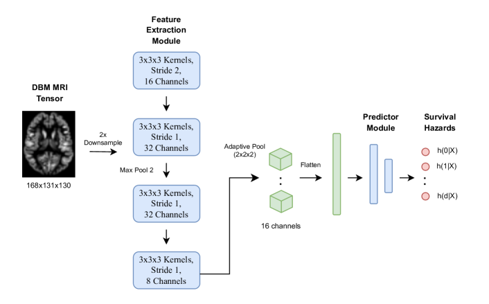
Figure 3: Architecture diagram of the shallow full brain 3D CNN model. 3D convolutional layers extract local volumetric features from the MRI DBM voxel tensor. Summary features from 8 sections of the tensor are collected and passed to a feed-forward predictor module to output the discrete conditional hazards.

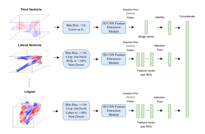
Figure 4: Architecture diagram of the region-based 3D CNN feature extraction. For each atlas region, the DBM voxels are cropped into $16\times 16\times 16$ regions of interest (ROIs) comprising at least 30% nonzero values, if the region is larger than this crop size. The ROIs are passed through a 3D CNN feature extractor, following the specs of the feature extraction module in Figure 3. The resulting tensors are spatially pooled and flattened to a feature vector for each ROI. The ROI feature vectors are pooled to a region-level feature vector using attention. Finally, the region-level feature vectors are concatenated to form the final DBM feature vector passed into the survival hazard predictor module from Figure 3. A separate feature extractor is learned jointly for each selected atlas region.

In contrast to the summary statistic featurization of the DBM data, 3D CNNs allow for flexible learning of localized features from the full brain or atlas region voxel-level tensors. Several applied works in MS have considered shallow 3D CNNs (Coll et al.,, 2024; Tousignant et al.,, 2019; Storelli et al.,, 2022). These relatively “parsimonious” architectures can be better suited to tasks with small sample size and without pretrained neural network weights to initialize the model with.

Our 3D CNN survival analysis pipeline, as applied to the full brain DBM tensor, is shown in Figure 3. After the original full brain tensor is downsampled, it is passed through four 3D convolutional layers with kernel size 3, followed by a spatial adaptive max pool. The features resulting from the pool are flattened to a vector and passed through a two layer fully connected predictor module, which outputs discrete survival hazards. The network is trained using the same log-likelihood loss function as described in Equation 2. All neural networks are trained using Pytorch 2.3.0 and Python 3.10.14.

We also train two additional CNN models from the literature, a deep convolutional attention model (CoAtNet), and a hierarchical transformer model designed for medical segmentation tasks (UNesT) (Dai et al.,, 2021; Yu et al.,, 2023). A 3D implementation of CoAtNet is used (Solovyev et al.,, 2022) and it is pretrained using ImageNet (Deng et al.,, 2009). For UNesT, the model is pretrained using T1-w MRIs. For both models, the final layer of their feature extractor modules are fed to an analogous predictor module as the in-house shallow architecture in Figure 3.

Finally, we propose a novel convolutional module to process a user selected subset of the atlas regions. This region-level convolutional model, which we refer to as Region CNN, permits the user to use domain knowledge or previous feature selection work to select a sparse set of regions for the CNN to completely focus on, rather than processing the full brain. The architecture for Region CNN is depicted in Figure 4. The user first specifies which regions are included in the model and separate CNN weights are then learned for each region. If the region is larger than $16\times 16\times 16$, it is cropped into regions of interest (ROIs) of this size, only keeping ROIs with sufficient ($>30\%)$ nonzero voxels. Otherwise, the region tensor is left as a single ROI. The region ROIs are passed through an analogous set of four 3D CNN layers as described in Figure 3. The only difference is that the stride of all CNN layers is 1. The resulting ROI feature vectors are collapsed to a single region-level feature vector using attention pooling (Vaswani et al.,, 2017). Finally, the region-level feature vectors are concatenated to form the DBM feature vector for the patient. For model training, this vector is processed through a predictor module in the same fashion as Figure 3.

3 Results and discussion

3.1 LOCO-MP feature selection

LOCO-MP identifies the most important DBM features for prediction in a stable manner. Each minipatch has dimension $n=N/5$ and $m=\sqrt{M}$, where $N=350$ and $M=56$. LOCO-MP was first applied to the entire dataset with $K=10000$ minipatches. RSF and CCDP24 were used as the prediction model and progression outcome, respectively. The first four columns of Table 2 show the regions, summary statistics (i.e., the features), feature importance scores $\bar{\Delta}_{j}$, and rankings of the top six features identified from applying LOCO-MP to the full dataset. Figure 1 in the Appendix shows this for all 56 features. In the following paragraphs, we demonstrate the robustness of these feature importance results through various stability checks.

Region	Summary Statistic	Full Data		Ten Subsamples
		Rank	$\bar{\Delta}_{j}$	Median Rank	Median $\bar{\Delta}_{j}$
3rd Ventricle	Std. Dev	1	0.00104	2	0.00090
Lateral Ventricle	Median	2	0.00101	1	0.00095
Precuneus	Median	3	0.00088	3	0.00078
Cerebellum White Matter	Median	4	0.00056	4	0.00064
Lingual	Median	5	0.00051	5	0.00061
Parahippocampal	Median	6	0.00051	6	0.00042

Table 2: Top six LOCO-MP selected features based on full data and ten subsamples. The feature occlusion scores ($\bar{\Delta}_{j}$) and full data/median subsample ranks are also shown.

Stability of LOCO-MP

In addition to the theoretical guarantees enjoyed by the LOCO-MP framework, we empirically validate its stability by testing its robustness against various data perturbations (Yu,, 2020; Yu and Barter,, 2024). We first assess the robustness of the feature importance list by generating ten 80% subsamples of the data and applying LOCO-MP to each subsample, collecting the corresponding feature importance scores ($\bar{\Delta}_{j}$) and rankings. This is shown in the latter two columns of Table 2. Despite a low signal-to-noise ratio in the DBM data, the top six features are identical between the full data and subsampled data models. The first two features are reversed in rank, but the difference in magnitude is extremely small (less than $0.00003$).

We measure the consistency of the feature rankings by computing the Jaccard similarity index $J$ between the ranks derived from the full dataset and those from the subsamples. This measures the proportion of overlap between two sets, ranging from 0 (no overlap) to 1 (complete overlap). By calculating $J$ for varying numbers of top-ranked features, we aimed to quantify how reliably the top features appeared in the subsampled rankings. Table 3 presents the results for the top 11 features from the full data model. Across the ten subsamples, the average and median values of $J$ decrease after six features before starting to plateau after ten. Therefore, we choose six as a heuristic number of DBM features to include in our model, though we demonstrate in Section 3.2 that our results remain relatively robust to varying numbers of top selected features.

Number of top features	2	3	4	5	6	7	8	9	10	11
Average $J$	0.93	0.85	0.84	1.00	0.94	0.80	0.89	0.77	0.72	0.68
Median $J$	1.00	1.00	1.00	1.00	1.00	0.75	0.89	0.80	0.67	0.69

Table 3: Summary of Jaccard index $J$ for increasing numbers of top features.

Permutation test

We tested the individual importance of the top DBM features by permuting their values across all patients and evaluating the ranks. For each feature, we permuted its values 25 times across patients and re-applied LOCO-MP for each permutation to evaluate the ranking of the permuted feature. The permutation disrupts the connections between individual DBM features and the outcomes/endpoints and tests whether higher ranks are attributable to specific feature identities. If the ranks of the permuted features are close to those from the unpermuted data, it would imply that the observed importance of the feature is not driven by the uniqueness of the feature (and corresponding brain region) itself. Instead, the perceived feature importance may be due to random and/or other global patterns in the data. The permuted ranks for each feature form a “pseudo-null distribution” under the null hypothesis that the feature is uninformative (shown as a violin plot in Figure 5). This allows us to assess how often permuted ranks are as low or lower than the original rank. The results are shown in Figure 5 – note that “Med” stands for the voxel median feature and “Sd” stands for the voxel standard deviation feature. For the top features identified by LOCO-MP, the ranks from the unpermuted models consistently fall below most, if not all of the permuted ranks, yielding a low “empirical p-value.” This suggests that the feature identities are indeed meaningful and unlikely due to chance, highlighting their potential relevance as medically important regions for MS progression, discussed in the last paragraph of this section.

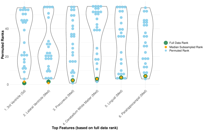
Figure 5: LOCO permutation test. We plot the distribution of top six LOCO-MP features after permuting their identities and re-applying LOCO-MP to each permutation. The $x$-axis shows the top six features and the $y$-axis shows the rank. “Med” stands for voxel median and “Sd” stands for voxel standard deviation. The green and orange points represent the full data and median subsampled ranks (both unpermuted), respectively. The light blue points represent the rank from a single permutation of that feature.

Benchmarking exercise

To assess the effectiveness of LOCO-MP, we benchmark it against a standard feature selection measurement that ranks features based on their feature importance scores from the random survival forest model. These scores are generated as average difference in out-of-bag prediction error across decision trees when the corresponding feature is permuted. We call this method “RF-Imp.” In principle, the bagging and feature subsets for each decision tree share some similarities with minipatch ensembling. Incorporating shuffled feature values onto already-trained decision trees can create large erroneous changes to predictions that would otherwise have fine performance if retrained without the feature. This may introduce unnecessary instability to RF-Imp when compared with LOCO-MP. Following the same procedure as LOCO-MP, we first compute RF-Imp feature importance scores from the full dataset and then on ten subsamples. Figure 6 shows the top six RF-Imp features based on the full data ranking. The blue boxplot shows the rank distribution across the ten subsamples, and the orange boxplot above it shows the corresponding LOCO-MP subsampled rank distribution for comparison.

Although there is alignment in the set of top regions captured between RF-Imp and LOCO-MP, the RF-Imp results alone demonstrate larger rank instability, especially beyond the third and lateral ventricles. In particular, the 5th and 6th ranked features differ between LOCO-MP and RF-Imp, but the top four are the same. It is clear that LOCO-MP has considerably lower variability in its rank distributions over the ten subsamples, establishing it as a more stable choice for feature selection. In contrast, the RF-Imp ranks have greater spread across subsamples, increasing the possibility of identifying spuriously meaningful features. The greater stability of LOCO-MP allows us to be more confident that the selected features are genuinely meaningful and not due to noise or other artifacts of the data.

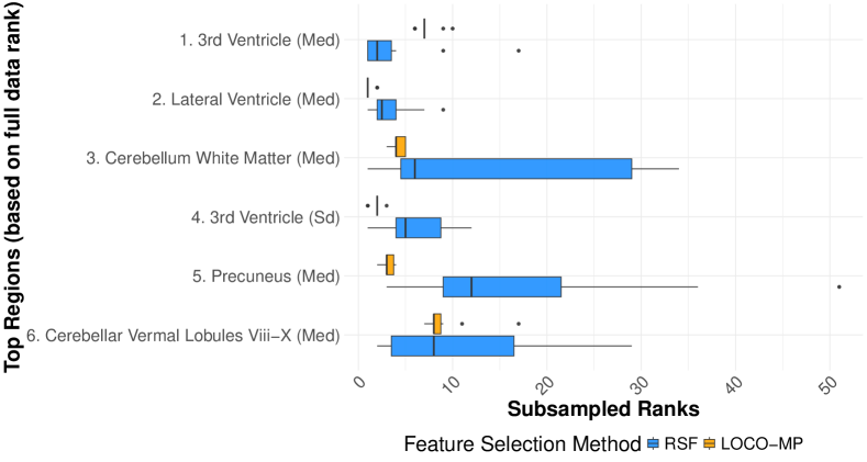
Figure 6: Rank distribution for RF-Imp feature importance (blue) vs LOCO-MP (orange). The $y$-axis shows the top six RF-Imp features in terms of their feature importance score from an RSF model applied to the full data. “Med” stands for voxel median and “Sd” stands for voxel standard deviation. The blue boxplots show their subsampled ranks on the $x$-axis. The orange boxplot above to each blue boxplot shows the rank distribution of that feature from LOCO-MP.

Clinical relevance of identified regions

In spite of the modestly sized LOCO-MP feature importance scores arising from the small cohort MRI data, the features and their ranks are stable. These features also align with brain regions that are clinically relevant in MS. The identified ventricular regions, including the third and lateral ventricles, are often indicated in MS progression studies (Müller et al.,, 2013; Guenter et al.,, 2022; Simon et al.,, 1999). Moreover, using the same trial data including the treatment arm, Song et al., (2022) identified significant treatment effects in the ventricular regions. The consistency across different studies emphasizes the robustness of the ventricle regions.

The cerebellum is also frequently indicated in MS studies (Weier et al.,, 2015; Brouwer et al.,, 2024), which may play a role in impairment of postural control and balance in MS patients (Gera et al.,, 2020). The precuneus and lingual gyrus are found abnormally activated in the brains of MS patients when performing cognitive exercises, and this activation was later associated with increased mental fatigue and slower speed in task completion (Chen et al.,, 2020). Finally, the parahippocampal gyrus (ranked 6th) has also been linked to varying activation patterns in MS patients compared to controls (Hulst et al.,, 2012), and is also associated with much greater lesion activity compared to controls (Geurts et al.,, 2007).

3.2 Prediction improvements using classical survival models

We show that the predictive models comprising LOCO-MP identified features have stronger discriminative power than models using all DBM features. We first present results from CCDP24, a canonical endpoint for measuring MS progression. We then discuss how the LOCO-MP selected features generalize well to alternative endpoints and compensate for the loss of key conventional predictors.

3.2.1 CCDP24 outcome

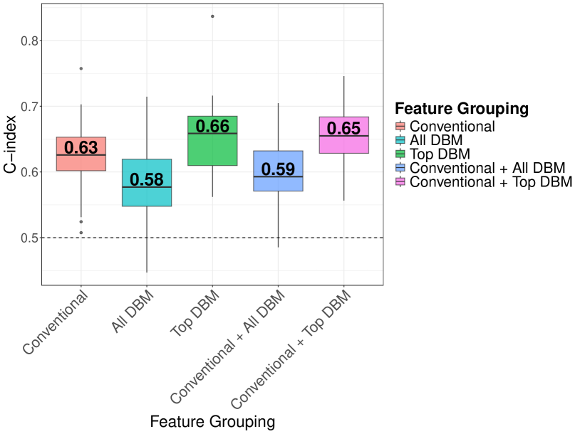
Figure 7: CCDP24 RSF model results. Boxplots show the distribution of random survival forest test-set C-indices across all cross-validation folds and repeats for outcome CCDP24. The $x$-axis consists of the feature groupings and the $y$-axis shows the test set C-indices. “Top DBM” refers to the top six DBM features. The annotated C-index represents the median value for a specific feature grouping.

Our RSF model results for the CCDP24 outcome are presented in Figure 7. Each boxplot shows the distribution of test-set C-indices for a specific feature grouping (discussed in Section 2.3) across all cross-validation folds and repeats. The median test-set C-index is annotated within each boxplot. Unsurprisingly, the “All DBM” model has the lowest C-index across the feature groups, likely due to overfitting from the high dimensionality of using all 56 DBM features. A similar conclusion can be drawn from the “Conventional + All DBM” model which includes even more features, showing how using an extensive set of MRI features without clinical context can lead to suboptimal predictive performance. These two models were slightly outperformed by the model using conventional features only, suggesting that the conventional features alone capture some degree of predictive value in CCDP24. In contrast, the two models that include the top features selected from DBM demonstrate the best prediction performance. Both C-indices are centered around 0.67, suggesting moderate predictive ability from the top DBM features. Adjusting for clinical information in the “Conventional + All/Top DBM” models did not appear to affect performance.

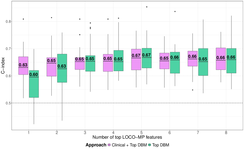
Figure 8: CCDP24 model stability. Boxplots show the distribution of CCDP24 test-set C-indices for the Conventional + Top DBM and Top DBM-only RSF models, plotted across varying numbers of top LOCO-MP features. The $x$-axis represents the number of top LOCO-MP features selected and the $y$-axis is the C-index.

For simplicity, the “Top DBM” models (Top DBM, Conventional + Top DBM) shown in Figure 7 are fit with the top six LOCO-MP features. However, the results from these two feature groupings remained stable with respect to varying numbers of LOCO-MP-selected features. Figure 8 plots the distribution of test-set C-indices from these two feature groupings across the top-ranked DBM features, ranging from 1 to 8. Performance remains stable across different numbers of features, suggesting that the model is robust to how many top features are used – the precise rankings between features and the specific number used for modeling is less important than identifying a broad set of features that can be investigated for clinical relevance. Although these two feature groupings are more investigative, researchers can be confident that the results are not overly sensitive to the specific subset of features. In Section 3.2.2, we discuss extending the LOCO-MP results to an alternative outcome to assess its generalizability.

Several conclusions can be drawn from our results. First, many of the DBM features contain overlapping information that ultimately results in model overfitting, as evidenced by the two “All DBM” model boxplots. This underscores the value of LOCO-MP, which can sift through highly correlated groups of features to identify the most prognostic ones and improve prediction performance. Moreover, the predictive strength of the DBM features and the clinical relevance of the corresponding brain regions reinforces the validity of these findings, demonstrating that LOCO-MP identifies DBM features with genuine predictive value.

3.2.2 25-foot walking test outcome

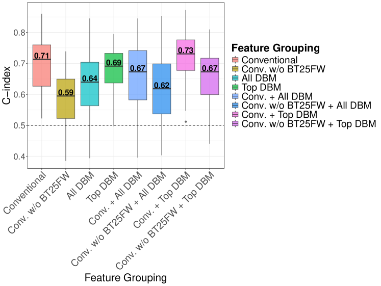
Figure 9: S25FW RSF model results. Boxplots show the distribution of random survival forest test-set C-indices across all cross-validation folds and repeats for outcome S25FW. The $x$-axis consists of the feature groupings and the $y$-axis shows the test set C-indices. “Top DBM” refers to the top six DBM features. The annotated C-index represents the median value for a specific feature grouping. We also include results after omitting the highly prognostic conventional variable BT25FW.

Despite variations in performance from across different feature sets, the CCDP24 C-indices are modest for even the strongest feature groups. This may arise from various factors, including inherent limitations in the outcome definition which impacts the model’s ability to identify meaningful signal – CCDP24 is characterized by marked changes in multiple events that are sustained for 24 weeks (Montalban et al.,, 2017; Krishnan et al.,, 2023). Although combining multiple events reduces the censoring rate, it comes at the cost of potentially introducing subjective measurements into the analysis: EDSS scoring can vary across studies, and the definition of EDSS-based progression highly depends on the study at hand (Krajnc et al.,, 2021). Therefore, including information from noisy outcome measurements could potentially worsen performance and we hypothesize this may be the case with CCDP24. To combat this, recent literature has pointed to the timed 25-foot walking test as an alternative measure of disability progression that may be more sensitive in detecting genuine disease worsening (Krajnc et al.,, 2021). This test measures the time for a patient to walk 25 feet without any assistive devices. Progression is defined as as a 20% increase in 25-foot walking time that is sustained for 24 weeks (S25FW). Previous studies have demonstrated significantly worse S25FW times in MS patients (Sikes et al.,, 2020) and S25FW has previously been shown to be strongly correlated with other forms of MS progression (Koch et al.,, 2020).

This outcome has a higher censoring rate compared to CCDP24 (88% compared to 77%), but resulted in higher C-indices across all feature groupings, shown in Figure 9. Similar to CCDP24, a model using all DBM features leads to overfitting. However, the conventional feature model demonstrates a 12.7% increase in median C-index compared to CCDP24 (0.63 to 0.71), and the “Conventional + Top DBM” and “Top DBM-only” models also see increases in median C-index. These increases suggest that DBM information is more effective in predicting S25FW-based progression. This also supports previously stated claims about the improved sensitivity of S25FW, illustrating the perils of using a noisy outcome measurement like CCDP24. The C-index for S25FW also remained robust to different numbers of top DBM features, as shown in Figure 10.

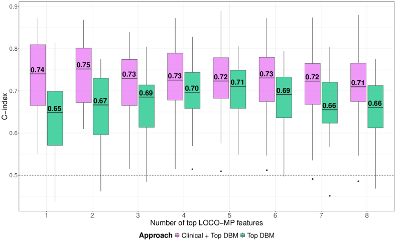
Figure 10: S25FW model stability. Boxplots show the distribution of S25FW test-set C-indices for the Conventional + Top DBM and Top DBM-only RSF models, plotted across varying numbers of top LOCO-MP features. The $x$-axis represents the number of top LOCO-MP features selected and the $y$-axis is the C-index.

The strong performance in the conventional model for S25FW is largely attributed to the baseline 25-foot walking test feature (BT25W, see Section 2.1) which is highly predictive of S25FW progression. The C-indices decrease after omitting BT25W as a conventional covariate in our models – the “Conventional-only” and “Conventional + All DBM” models achieve a median C-index of 0.59 and 0.62, respectively, as shown in Figure 9. These performances are comparable to their CCDP24 counterparts. While omitting BT25FW results in worse performance across all feature groupings with conventional features, the “Conventional + Top DBM” model performs fairly robustly even after omitting BT25FW, achieving a median C-index of 0.67. This demonstrates that the top DBM features may be able to compensate for the loss of key conventional predictors and shows how LOCO-MP can identify robust and generalizable features.

We also note that the two “Top DBM” models in the S25FW analysis use LOCO-MP features identified from the CCDP24 outcome – the algorithm encountered challenges when applied to S25FW due to its high censoring rate, which limited the number of informative minipatches (many minipatches consisted entirely of censored patients). Despite this, the increased performance in the two “Top DBM” S25FW models demonstrates the reliability of LOCO-MP in identifying a stable feature set that captures fundamental aspects of disease progression that are robust across different outcome definitions. This strong generalization is further evidence that the top features may be genuine markers of disease worsening, enhancing its potential for broader clinical applications and underscoring the value of DBM as a regional identification framework.

While this new outcome allowed for more precise patient risk discrimination, the variance of the C-index estimates was higher than that of CCDP24. This is due to the higher censoring rate in S25FW which, by reducing the number of informative events, lowers the effective sample size. This generally leads to increased variance in the estimates because there is less observed data available to accurately capture the underlying risk. Even though S25FW provides clearer risk stratification, the higher variation in the C-index reflects the statistical challenges introduced by a lower effective sample size. In contrast, the CCDP24 outcome has lower variance but lower C-indices as well. It remains an area of future work to create disease measures that are both sensitive and characterized by large sample sizes.

We also observe that the test set C-indices for the strongest feature groupings primarily range between 0.6-0.7, reflecting moderately strong performance at best. These magnitudes are not unexpected given the noisy data regime of the DBM voxels and the low feature importance scores from LOCO-MP, which constrain the predictive power of the DBM features. However, the goal of our study is to evaluate the incremental value of the DBM features as opposed to arguing about the predictive strength of survival models with DBM compared to other MRI imaging features, such as T2 lesion volume or cortical thickness. While DBM features may not outperform these modalities in terms of predictive accuracy, they uniquely capture subtle volumetric abnormalities across the brain and provide orthogonal information to the conventional features. Our models demonstrate how, even in a low-signal regime, DBM features contribute to MS progression in a way that is stable and clinically meaningful, even if their predictive performance may be outperformed by MRI modalities not considered in our study. Future work could explore integrating DBM with well-established MRI modalities to fully assess the strength of each one.

3.3 Prediction improvements using convolutional neural networks

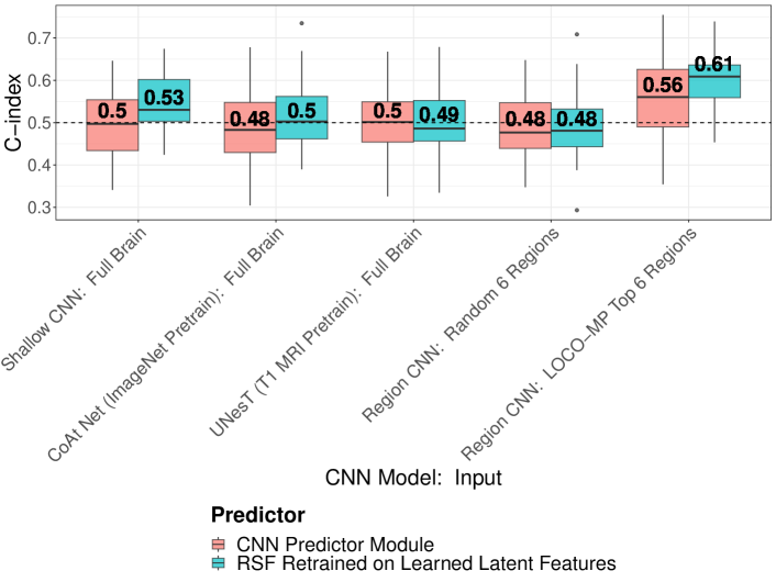
Figure 11: CNN model performance for CCDP24. Boxplots show the distribution of test C-indices for each of the tested CNN models. Results are presented both for the trained CNN predictor module (CNN Predictor Module), as well as an RSF trained on the extracted feature vector of each trained CNN (RF Retrained on Extracted Features). The $x$-axis labels first give the CNN model architecture used, followed by the inputs used. Specifically, full brain models are compared with Region CNN, using either the top 6 LOCO-MP regions or random 6 regions (excluding 6 LOCO-MP regions) with each fold.

We compare full brain CNNs against Region CNN using only the top 6 identified LOCO-MP regions to assess the extent to which an unsupervised deep learning feature extraction improves prediction performance. Figure 11 presents CNN model test C-indices over 30 80%/20% data splits for predicting CCDP24. The evaluated models include the three baseline full brain models (Shallow, CoAtNet UNesT), Region CNN trained on the top 6 LOCO-MP regions, and Region CNN trained on 6 randomly selected regions (excluding the top 6 LOCO-MP regions). Each of these models are described in Section 2.4. Red boxplots show the C-index distribution from the predictions of the CNN predictor module. The learned latent features from each CNN (i.e., the concatenated green bar in Figure 3) were also extracted and retrained using a conventional RSF survival model (without conventional features), enabling the continuous survival times to be used as the outcome. Teal boxplots show the C-index distribution of the RSF models trained on these extracted CNN feature vectors.

These results underscore the importance of subsetting the DBM input to the top 6 LOCO-MP regions in order to extract signal from a CNN. Each of the full brain CNN models struggle to achieve nonrandom performance (C-index $\geq 0.5$). The shallow full brain CNN features perform modestly better than the complex CoAtNet and UNesT architectures. This suggests that, for this data and cohort size, neither an attention mechanism nor a very deep architecture are able to adequately predict CCDP24. Additionally, CoAtNet was pretrained using ImageNet (Deng et al.,, 2009) and UNesT was pretrained using raw T1-w MRI tensors, indicating that the DBM data may reflect critically different patterns than the raw MRI. Region CNN fares quite poorly when trained on 6 random non-LOCO-MP regions. However, it extracts strong predictive signal when LOCO-MP features are used. The LOCO-MP features were more helpful in the RSF model, achieving a median C-index of 0.61. Region CNN with the top 6 LOCO-MP regions performs comparably on the S25FW outcome (median predictor module C-Index: $0.57$; median RSF retrained C-Index: $0.61$). Ultimately, even the best CNN fares moderately worse than the corresponding classical survival model in Section 3.2, highlighting the challenge of learning complex models for the DBM data on this cohort size. With more data, Region CNN (and CNNs generally) may be able to extract more expressive features from the T1-w MRI data.

4 Conclusion

Identifying predictive and biologically meaningful features in medical studies is an important step towards developing targeted patient interventions and deepening our understanding of disease mechanisms. In this paper, we demonstrate how statistical and machine learning methods can be utilized with DBM to gain meaningful insights about brain regions and their role in predicting MS progression. First, we extend a model-agnostic feature importance method (LOCO-MP) to survival analysis. Using DBM data, we show that LOCO-MP identifies multiple clinically relevant features in a stable manner, outperforming other feature importance metrics. To assess the prognostic value of these features, we fit survival models with various feature groupings that include combinations of conventional and DBM features. We also develop a 3D CNN architecture, Region CNN, that processes a preselected subset of the atlas regions. Our findings indicate that the top DBM features play a valuable role in improving prediction performance, alone or when combined with conventional features. To verify that the selected features can generalize to other outcomes, we tested their performance across alternative outcomes and observed that the models retained strong predictive accuracy.

While our results are specific to this study cohort, the analysis pipeline we develop is general and can be broadly applied to any DBM dataset. Further analyses using external data can develop a more confident scientific understanding about how regional volumetric changes contribute to MS disease worsening. Concerning prediction, our study explored how the DBM features could improve our understanding and prediction of MS progression rather than make definitive claims about model performance. Our findings provide an optimistic and practical benchmark for the prognostic utility of DBM in MS prediction tasks. More complex and principled machine learning frameworks could better contextualize the predictive power of DBM features. Larger cohort sizes of DBM data can additionally enable exploration of whether CNNs can outperform classical approaches, creating the potential for DBM pretrained models.

We evaluated the generalizability of the selected LOCO-MP features by using them to predict a different progression outcome. However, both outcomes were based on 24-week sustained progression measurements which focuses on short-term rather than long-term disease worsening. If the latter is of greater interest, then longitudinal modeling may give insights into whether DBM measurements taken over time are helpful.

Ultimately, our study demonstrates the promise of DBM as a tool for identifying key features and improving MS prediction models. The ability to pinpoint clinically meaningful features in a low-signal regime demonstrates the potential of developing DBM-based biomarkers that can inform therapeutic development and potentially improve efficiency in later MS clinical trials. By integrating DBM with statistical and machine learning frameworks, we provide an analysis pipeline that balances stability, predictive performance, and domain-level interpretability to provide valuable insights to the medical imaging and multiple sclerosis fields.

Acknowledgments and funding

Andy Shen is partially supported by the National Science Foundation (NSF) Graduate Research Fellowship under Grant No. 2146752. Any opinion, findings, and conclusions or recommendations expressed in this material are those of the authors(s) and do not necessarily reflect the views of the NSF. This project was supported by Genentech/Roche.

Declaration of competing interest

Richard A.D. Carano and Zhuang Song are employees of Genentech/Roche and are stockholders of Roche.

Data availability statement

The fully anonymized, individual patient raw data including clinical and MRI data of the OPERA trials are made available through the International Progressive MS Alliance (www.progressivemsalliance.org).

Supplementary Materials:
Assessing the Role of Volumetric Brain Information in Multiple Sclerosis Progression

Appendix A Additional LOCO-MP and feature selection results

Figure 1 shows boxplots for all 56 DBM features, similar to Figure 6 in the main text. Blue boxplots show the rank distribution from RF-Imp while orange boxplots show the rank distribution from LOCO-MP.

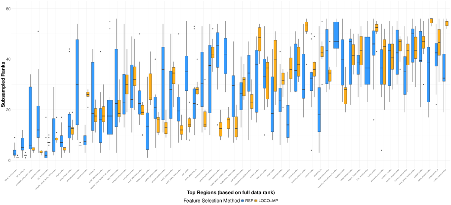
Figure 1: Rank distribution for RSF feature importance (blue) vs LOCO-MP (orange) for all DBM features. The $x$-axis shows the features (from highest to lowest rank) in terms of their feature importance score from an RSF model applied to the full data, and the blue boxplots show their subsampled ranks on the $y$-axis. The orange boxplot next to each blue boxplot shows the rank distribution of that feature from LOCO-MP.

Table 1 shows the LOCO-MP feature importance scores for all 56 DBM features.

Region	Full Data		Subsamples
	Rank	$\bar{\Delta}_{j}$	Median Rank	Median $\bar{\Delta}_{j}$
3rd Ventricle SD	1	0.00104	2	0.00090
Lateral Ventricle Median	2	0.00101	1	0.00095
Precuneus Median	3	0.00088	3	0.00078
Cerebellum White Matter Median	4	0.00056	4	0.00064
Lingual Median	5	0.00051	5	0.00061
Parahippocampal Median	6	0.00051	6	0.00042
Cerebellar Vermal Lobules VIII-X Median	7	0.00029	8	0.00027
3rd Ventricle Median	8	0.00028	7	0.00037
Basal Forebrain Median	9	0.00026	12.5	0.00016
Caudal Anterior Cingulate Median	10	0.00023	16	0.00014
Caudal Middle Frontal Median	11	0.00017	12.5	0.00019
Supramarginal Median	12	0.00016	12.5	0.00017
Rostral Middle Frontal Median	13	0.00016	12	0.00019
CSF Median	14	0.00015	14	0.00015
Lateral Orbitofrontal Median	15	0.00014	19	0.00008
Posterior Cingulate Median	16	0.00014	13	0.00017
Pars Orbitalis Median	17	0.00012	18.5	0.00008
Caudate SD	18	0.00010	17.5	0.00009
Medial Orbitofrontal Median	19	0.00005	17.5	0.00008
Paracentral Median	20	0.00004	26	-0.00002
Pericalcarine Median	21	0.00003	32	-0.00010
Superior Parietal Median	22	0.00002	16	0.00014
Cerebellum Exterior Median	23	-0.00000	30	-0.00007
Entorhinal Median	24	-0.00002	14	0.00014
Amygdala Median	25	-0.00002	28	-0.00003
Brain Stem Median	26	-0.00003	36.5	-0.00014
Rostral Anterior Cingulate Median	27	-0.00003	23	0.00001
Lateral Occipital Median	28	-0.00005	34.5	-0.00011
Isthmus Cingulate Median	29	-0.00005	25	-0.00002
Pars Triangularis Median	30	-0.00006	42	-0.00021
Superior Frontal Median	31	-0.00007	43.5	-0.00021
Pars Opercularis Median	32	-0.00008	32	-0.00007
Lateral Orbitofrontal SD	33	-0.00010	28	-0.00005
Hippocampus Median	34	-0.00010	34.5	-0.00011
Cerebellar Vermal Lobules I-V Median	35	-0.00010	25.5	-0.00003
Caudate Median	36	-0.00012	36	-0.00012
Fusiform Median	37	-0.00012	36	-0.00015
Accumbens Area Median	38	-0.00013	45	-0.00022
Insula Median	39	-0.00019	40	-0.00020
Inferior Parietal Median	40	-0.00019	41.5	-0.00019
Postcentral Median	41	-0.00019	31.5	-0.00010
Pallidum Median	42	-0.00020	47	-0.00023
Ventral DC Median	43	-0.00020	40.5	-0.00018
Precentral Median	44	-0.00023	38	-0.00016
Transverse Temporal Median	45	-0.00023	53.5	-0.00035
Cerebellar Vermal Lobules VI-VII Median	46	-0.00024	49	-0.00026
Putamen Median	47	-0.00025	48.5	-0.00027
Lateral Ventricle SD	48	-0.00025	46.5	-0.00024
4th Ventricle Median	49	-0.00025	45.5	-0.00024
Inferior Lateral Ventricle Median	50	-0.00026	43.5	-0.00021
Superior Temporal Median	51	-0.00026	47	-0.00023
Paracentral SD	52	-0.00029	42.5	-0.00020
Cuneus Median	53	-0.00033	52.5	-0.00033
Thalamus Proper Median	54	-0.00035	43.5	-0.00022
Inferior Temporal Median	55	-0.00047	55	-0.00041
Middle Temporal Median	56	-0.00052	56	-0.00046

Table 1: Feature importance scores and rankings from full data and subsamples for all 56 high-variance VoxelDBM regions.

Appendix B Cox proportional hazards modeling

Figures 2 and 3 show the distribution of test set C-indices across all folds for each feature group when a penalized Cox proportional hazards model (ridge penalty) is used to predict progression. Figure 2 uses the CCDP24 outcome and Figure 3 uses the 25-foot walking outcome.

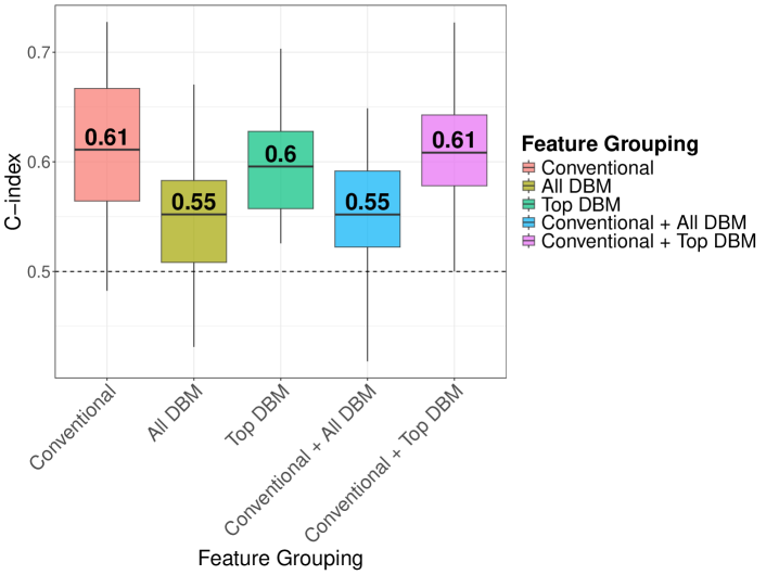
Figure 2: CCDP24 Cox model results. Boxplots show the distribution of penalized Cox proportional hazards model (ridge penalty) test-set C-indices across all cross-validation folds and repeats for outcome CCDP24. The $x$-axis consists of the five feature groupings and the $y$-axis shows the test set C-indices. “Top MRI” refers to the top five DBM features. The annotated C-index represents the median value for a specific feature grouping.

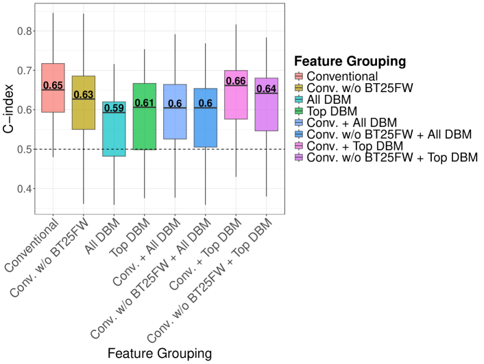
Figure 3: S25FW Cox model results. Boxplots show the distribution of penalized Cox proportional hazards model (ridge penalty) test-set C-indices across all cross-validation folds and repeats for outcome 25FW. The $x$-axis consists of the five feature groupings and the $y$-axis shows the test set C-indices. “Top MRI” refers to the top five DBM features. The annotated C-index represents the median value for a specific feature grouping.

Figures 4 and 5 show the stability of the test set C-indices across varying numbers of top LOCO-MP features for the penalized Cox proportional hazards model (ridge penalty). Figure 4 uses the CCDP24 outcome and Figure 5 uses the 25FW outcome.

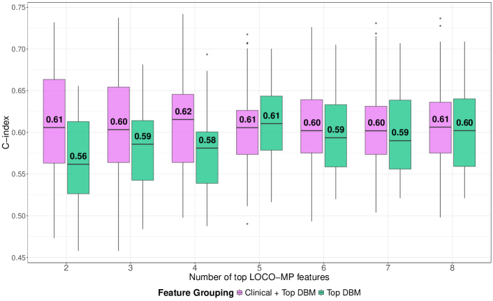
Figure 4: CCDP24 Cox model stability. Boxplots show the distribution of CCDP24 test-set C-indices for the conventional + top MRI and top MRI-only Cox proportional hazard (ridge) models, plotted across varying numbers of top LOCO-MP features. The $x$-axis represents the number of top LOCO-MP features selected and the $y$-axis is the C-index.

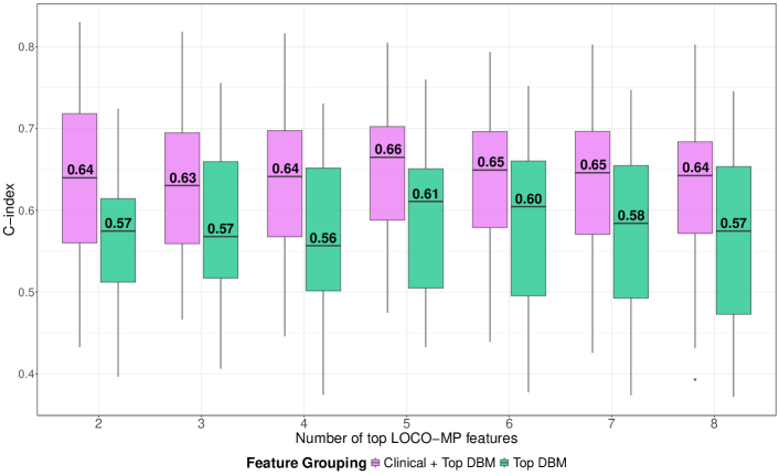
Figure 5: S25FW Cox model stability. Boxplots show the distribution of S25FW test-set C-indices for the conventional + top MRI and top MRI-only Cox proportional hazards (ridge penalty) models, plotted across varying numbers of top LOCO-MP features. The $x$-axis represents the number of top LOCO-MP features selected and the $y$-axis is the C-index.

References

- Agarwal et al., (2023) Agarwal, A., Kenney, A. M., Tan, Y. S., Tang, T. M., and Yu, B. (2023). Mdi+: A flexible random forest-based feature importance framework. arXiv preprint arXiv:2307.01932.
- Ashburner et al., (1998) Ashburner, J., Hutton, C., Frackowiak, R., Johnsrude, I., Price, C., and Friston, K. (1998). Identifying global anatomical differences: Deformation-based morphometry. Human brain mapping, 6(5-6):348–357.
- Azevedo et al., (2018) Azevedo, C. J., Cen, S. Y., Khadka, S., Liu, S., Kornak, J., Shi, Y., Zheng, L., Hauser, S. L., and Pelletier, D. (2018). Thalamic atrophy in multiple sclerosis: a magnetic resonance imaging marker of neurodegeneration throughout disease. Annals of neurology, 83(2):223–234.
- Bar-Or et al., (2023) Bar-Or, A., Thanei, G.-A., Harp, C., Bernasconi, C., Bonati, U., Cross, A. H., Fischer, S., Gaetano, L., Hauser, S. L., Hendricks, R., et al. (2023). Blood neurofilament light levels predict non-relapsing progression following anti-cd20 therapy in relapsing and primary progressive multiple sclerosis: findings from the ocrelizumab randomised, double-blind phase 3 clinical trials. EBioMedicine, 93.
- Bergsland et al., (2018) Bergsland, N., Horakova, D., Dwyer, M., Uher, T., Vaneckova, M., Tyblova, M., Seidl, Z., Krasensky, J., Havrdova, E., and Zivadinov, R. (2018). Gray matter atrophy patterns in multiple sclerosis: A 10-year source-based morphometry study.
- Bermel and Bakshi, (2006) Bermel, R. A. and Bakshi, R. (2006). The measurement and clinical relevance of brain atrophy in multiple sclerosis. The Lancet Neurology, 5(2):158–170.
- Breiman et al., (2018) Breiman, L., Cutler, A., Liaw, A., and Wiener, M. (2018). Package ‘randomforest’. University of California, Berkeley: Berkeley, CA, USA.
- Brouwer et al., (2024) Brouwer, E. J., Strik, M., and Schoonheim, M. M. (2024). The role of the cerebellum in multiple sclerosis: structural damage and disconnecting networks. Current Opinion in Behavioral Sciences, 59:101436.
- Cadavid et al., (2017) Cadavid, D., Cohen, J. A., Freedman, M. S., Goldman, M. D., Hartung, H.-P., Havrdova, E., Jeffery, D., Kapoor, R., Miller, A., Sellebjerg, F., et al. (2017). The edss-plus, an improved endpoint for disability progression in secondary progressive multiple sclerosis. Multiple Sclerosis Journal, 23(1):94–105.
- Chard et al., (2002) Chard, D., Griffin, C., Parker, G., Kapoor, R., Thompson, A., and Miller, D. (2002). Brain atrophy in clinically early relapsing–remitting multiple sclerosis. Brain, 125(2):327–337.
- Chen et al., (2020) Chen, M. H., Wylie, G. R., Sandroff, B. M., Dacosta-Aguayo, R., DeLuca, J., and Genova, H. M. (2020). Neural mechanisms underlying state mental fatigue in multiple sclerosis: a pilot study. Journal of Neurology, 267:2372–2382.
- Chung et al., (2001) Chung, M. K., Worsley, K. J., Paus, T., Cherif, C., Collins, D. L., Giedd, J. N., Rapoport, J. L., and Evans, A. C. (2001). A unified statistical approach to deformation-based morphometry. NeuroImage, 14(3):595–606.
- Coll et al., (2024) Coll, L., Pareto, D., Carbonell-Mirabent, P., Cobo-Calvo, Á., Arrambide, G., Vidal-Jordana, Á., Comabella, M., Castilló, J., Rodriguez-Acevedo, B., Zabalza, A., et al. (2024). Global and regional deep learning models for multiple sclerosis stratification from mri. Journal of Magnetic Resonance Imaging, 60(1):258–267.
- Compston and Coles, (2008) Compston, A. and Coles, A. (2008). Multiple sclerosis. The Lancet, 372(9648):1502–1517.
- Dai et al., (2021) Dai, Z., Liu, H., Le, Q. V., and Tan, M. (2021). Coatnet: Marrying convolution and attention for all data sizes. Advances in neural information processing systems, 34:3965–3977.
- Deng et al., (2009) Deng, J., Dong, W., Socher, R., Li, L.-J., Li, K., and Fei-Fei, L. (2009). Imagenet: A large-scale hierarchical image database. In 2009 IEEE conference on computer vision and pattern recognition, pages 248–255. Ieee.
- Elliott et al., (2019) Elliott, C., Belachew, S., Wolinsky, J. S., Hauser, S. L., Kappos, L., Barkhof, F., Bernasconi, C., Fecker, J., Model, F., Wei, W., et al. (2019). Chronic white matter lesion activity predicts clinical progression in primary progressive multiple sclerosis. Brain, 142(9):2787–2799.
- Fisniku et al., (2008) Fisniku, L. K., Chard, D. T., Jackson, J. S., Anderson, V. M., Altmann, D. R., Miszkiel, K. A., Thompson, A. J., and Miller, D. H. (2008). Gray matter atrophy is related to long-term disability in multiple sclerosis. Annals of Neurology: Official Journal of the American Neurological Association and the Child Neurology Society, 64(3):247–254.
- Friedman et al., (2021) Friedman, J., Hastie, T., Tibshirani, R., Narasimhan, B., Tay, K., Simon, N., and Qian, J. (2021). Package ‘glmnet’. CRAN R Repositary, 595.
- Gan and Allen, (2022) Gan, L. and Allen, G. I. (2022). Fast and interpretable consensus clustering via minipatch learning. PLOS Computational Biology, 18(10):e1010577.
- Gan et al., (2023) Gan, L., Zheng, L., and Allen, G. I. (2023). Model-agnostic confidence intervals for feature importance: A fast and powerful approach using minipatch ensembles.
- Gera et al., (2020) Gera, G., Fling, B. W., and Horak, F. B. (2020). Cerebellar white matter damage is associated with postural sway deficits in people with multiple sclerosis. Archives of Physical Medicine and Rehabilitation, 101(2):258–264.
- Geurts et al., (2007) Geurts, J. J., Bö, L., Roosendaal, S. D., Hazes, T., Daniëls, R., Barkhof, F., Witter, M. P., Huitinga, I., and van der Valk, P. (2007). Extensive hippocampal demyelination in multiple sclerosis. Journal of Neuropathology & Experimental Neurology, 66(9):819–827.
- Guenter et al., (2022) Guenter, W., Betscher, E., and Bonek, R. (2022). Predictive value of the third ventricle width for neurological status in multiple sclerosis. Journal of Clinical Medicine, 11(10):2841.
- Hauser et al., (2017) Hauser, S. L., Bar-Or, A., Comi, G., Giovannoni, G., Hartung, H.-P., Hemmer, B., Lublin, F., Montalban, X., Rammohan, K. W., Selmaj, K., et al. (2017). Ocrelizumab versus interferon beta-1a in relapsing multiple sclerosis. New England Journal of Medicine, 376(3):221–234.
- Hulst et al., (2012) Hulst, H. E., Schoonheim, M. M., Roosendaal, S. D., Popescu, V., Schweren, L. J., van der Werf, Y. D., Visser, L. H., Polman, C. H., Barkhof, F., and Geurts, J. J. (2012). Functional adaptive changes within the hippocampal memory system of patients with multiple sclerosis. Human brain mapping, 33(10):2268–2280.
- Ishwaran and Kogalur, (2019) Ishwaran, H. and Kogalur, U. B. (2019). Fast unified random forests for survival, regression, and classification (rf-src). R package version, 2(1).
- Ishwaran et al., (2008) Ishwaran, H., Kogalur, U. B., Blackstone, E. H., and Lauer, M. S. (2008). Random survival forests.
- Klein et al., (2017) Klein, A., Ghosh, S. S., Bao, F. S., Giard, J., Häme, Y., Stavsky, E., Lee, N., Rossa, B., Reuter, M., Chaibub Neto, E., et al. (2017). Mindboggling morphometry of human brains. PLoS computational biology, 13(2):e1005350.
- Koch et al., (2020) Koch, M. W., Mostert, J., Uitdehaag, B., and Cutter, G. (2020). Clinical outcome measures in spms trials: An analysis of the impact and ascend original trial data sets. Multiple Sclerosis Journal, 26(12):1540–1549.
- Krajnc et al., (2021) Krajnc, N., Berger, T., and Bsteh, G. (2021). Measuring treatment response in progressive multiple sclerosis—considerations for adapting to an era of multiple treatment options. Biomolecules, 11(9):1342.
- Krishnan et al., (2023) Krishnan, A. P., Song, Z., Clayton, D., Jia, X., de Crespigny, A., and Carano, R. A. (2023). Multi-arm u-net with dense input and skip connectivity for t2 lesion segmentation in clinical trials of multiple sclerosis. Scientific Reports, 13(1):4102.
- Lei and Wasserman, (2014) Lei, J. and Wasserman, L. (2014). Distribution-free prediction bands for non-parametric regression. Journal of the Royal Statistical Society Series B: Statistical Methodology, 76(1):71–96.
- Lomer et al., (2024) Lomer, N. B., Asalemi, K. A., Saberi, A., and Sarlak, K. (2024). Predictors of multiple sclerosis progression: A systematic review of conventional magnetic resonance imaging studies. Plos one, 19(4):e0300415.
- Manjón et al., (2010) Manjón, J. V., Coupé, P., Martí-Bonmatí, L., Collins, D. L., and Robles, M. (2010). Adaptive non-local means denoising of mr images with spatially varying noise levels. Journal of Magnetic Resonance Imaging, 31(1):192–203.
- Moazami et al., (2021) Moazami, F., Lefevre-Utile, A., Papaloukas, C., and Soumelis, V. (2021). Machine learning approaches in study of multiple sclerosis disease through magnetic resonance images. Frontiers in immunology, 12:700582.
- Montalban et al., (2017) Montalban, X., Hauser, S. L., Kappos, L., Arnold, D. L., Bar-Or, A., Comi, G., De Seze, J., Giovannoni, G., Hartung, H.-P., Hemmer, B., et al. (2017). Ocrelizumab versus placebo in primary progressive multiple sclerosis. New england journal of medicine, 376(3):209–220.
- Müller et al., (2013) Müller, M., Esser, R., Kötter, K., Voss, J., Müller, A., and Stellmes, P. (2013). Third ventricular enlargement in early stages of multiple sclerosis is a predictor of motor and neuropsychological deficits: a cross-sectional study. BMJ open, 3(9):e003582.
- Pellegrini et al., (2020) Pellegrini, F., Copetti, M., Sormani, M. P., Bovis, F., de Moor, C., Debray, T. P., and Kieseier, B. C. (2020). Predicting disability progression in multiple sclerosis: insights from advanced statistical modeling. Multiple Sclerosis Journal, 26(14):1828–1836.
- Pisani et al., (2021) Pisani, A. I., Scalfari, A., Crescenzo, F., Romualdi, C., and Calabrese, M. (2021). A novel prognostic score to assess the risk of progression in relapsing- remitting multiple sclerosis patients. European journal of neurology, 28(8):2503–2512.
- Prathapan et al., (2024) Prathapan, V., Eipert, P., Wigger, N., Kipp, M., Appali, R., and Schmitt, O. (2024). Modeling and simulation for prediction of multiple sclerosis progression: A review and perspective. Computers in Biology and Medicine, page 108416.
- Rocca et al., (2021) Rocca, M. A., Anzalone, N., Storelli, L., Del Poggio, A., Cacciaguerra, L., Manfredi, A. A., Meani, A., and Filippi, M. (2021). Deep learning on conventional magnetic resonance imaging improves the diagnosis of multiple sclerosis mimics. Investigative Radiology, 56(4):252–260.
- Rocca et al., (2019) Rocca, M. A., Preziosa, P., and Filippi, M. (2019). Application of advanced mri techniques to monitor pharmacologic and rehabilitative treatment in multiple sclerosis: current status and future perspectives. Expert Review of Neurotherapeutics, 19(9):835–866.
- Shao et al., (2023) Shao, Z., Chen, Y., Bian, H., Zhang, J., Liu, G., and Zhang, Y. (2023). Hvtsurv: Hierarchical vision transformer for patient-level survival prediction from whole slide image. In Proceedings of the AAAI Conference on Artificial Intelligence, volume 37, pages 2209–2217.
- Sikes et al., (2020) Sikes, E. M., Cederberg, K. L., Sandroff, B. M., Bartolucci, A., and Motl, R. W. (2020). Quantitative synthesis of timed 25-foot walk performance in multiple sclerosis. Archives of Physical Medicine and Rehabilitation, 101(3):524–534.
- Simon et al., (1999) Simon, J., Jacobs, L., Campion, M., Rudick, R., Cookfair, D., Herndon, R., Richert, J., Salazar, A., Fischer, J., Goodkin, D., et al. (1999). A longitudinal study of brain atrophy in relapsing multiple sclerosis. Neurology, 53(1):139–139.
- Solovyev et al., (2022) Solovyev, R., Kalinin, A. A., and Gabruseva, T. (2022). 3d convolutional neural networks for stalled brain capillary detection. Computers in Biology and Medicine, 141:105089.
- Song et al., (2022) Song, Z., Krishnan, A., Gaetano, L., Tustison, N. J., Clayton, D., de Crespigny, A., Bengtsson, T., Jia, X., and Carano, R. A. (2022). Deformation-based morphometry identifies deep brain structures protected by ocrelizumab. NeuroImage: Clinical, 34:102959.
- Sormani et al., (2010) Sormani, M., Bonzano, L., Roccatagliata, L., Mancardi, G., Uccelli, A., and Bruzzi, P. (2010). Surrogate endpoints for edss worsening in multiple sclerosis: a meta-analytic approach. Neurology, 75(4):302–309.
- Storelli et al., (2022) Storelli, L., Azzimonti, M., Gueye, M., Vizzino, C., Preziosa, P., Tedeschi, G., De Stefano, N., Pantano, P., Filippi, M., and Rocca, M. A. (2022). A deep learning approach to predicting disease progression in multiple sclerosis using magnetic resonance imaging. Investigative Radiology, 57(7):423–432.
- Tousignant et al., (2019) Tousignant, A., Lemaître, P., Precup, D., Arnold, D. L., and Arbel, T. (2019). Prediction of disease progression in multiple sclerosis patients using deep learning analysis of mri data. In International conference on medical imaging with deep learning, pages 483–492. PMLR.
- Tustison et al., (2010) Tustison, N. J., Avants, B. B., Cook, P. A., Zheng, Y., Egan, A., Yushkevich, P. A., and Gee, J. C. (2010). N4itk: improved n3 bias correction. IEEE transactions on medical imaging, 29(6):1310–1320.
- Tustison et al., (2019) Tustison, N. J., Holbrook, A. J., Avants, B. B., Roberts, J. M., Cook, P. A., Reagh, Z. M., Duda, J. T., Stone, J. R., Gillen, D. L., Yassa, M. A., et al. (2019). Longitudinal mapping of cortical thickness measurements: An alzheimer’s disease neuroimaging initiative-based evaluation study. Journal of Alzheimer’s Disease, 71(1):165–183.
- Vale-Silva and Rohr, (2021) Vale-Silva, L. A. and Rohr, K. (2021). Long-term cancer survival prediction using multimodal deep learning. Scientific Reports, 11(1):13505.
- Vaswani et al., (2017) Vaswani, A., Shazeer, N., Parmar, N., Uszkoreit, J., Jones, L., Gomez, A. N., Kaiser, L. u., and Polosukhin, I. (2017). Attention is all you need. In Guyon, I., Luxburg, U. V., Bengio, S., Wallach, H., Fergus, R., Vishwanathan, S., and Garnett, R., editors, Advances in Neural Information Processing Systems, volume 30. Curran Associates, Inc.
- Vázquez-Marrufo et al., (2022) Vázquez-Marrufo, M., Sarrias-Arrabal, E., García-Torres, M., Martín-Clemente, R., and Izquierdo, G. (2022). A systematic review of the application of machine-learning algorithms in multiple sclerosis. Neurología (English Edition).
- Weier et al., (2015) Weier, K., Banwell, B., Cerasa, A., Collins, D. L., Dogonowski, A.-M., Lassmann, H., Quattrone, A., Sahraian, M. A., Siebner, H. R., and Sprenger, T. (2015). The role of the cerebellum in multiple sclerosis. The Cerebellum, 14:364–374.
- Yao and Allen, (2021) Yao, T. and Allen, G. I. (2021). Feature selection for huge data via minipatch learning.
- Yu, (2020) Yu, B. (2020). Veridical data science. In Proceedings of the 13th international conference on web search and data mining, pages 4–5.
- Yu and Barter, (2024) Yu, B. and Barter, R. L. (2024). Veridical data science: The practice of responsible data analysis and decision making. MIT Press.
- Yu et al., (2023) Yu, X., Yang, Q., Zhou, Y., Cai, L. Y., Gao, R., Lee, H. H., Li, T., Bao, S., Xu, Z., Lasko, T. A., et al. (2023). Unest: local spatial representation learning with hierarchical transformer for efficient medical segmentation. Medical Image Analysis, 90:102939.
- Zadeh and Schmid, (2020) Zadeh, S. G. and Schmid, M. (2020). Bias in cross-entropy-based training of deep survival networks. IEEE transactions on pattern analysis and machine intelligence, 43(9):3126–3137.
- Zhang et al., (2023) Zhang, K., Lincoln, J. A., Jiang, X., Bernstam, E. V., and Shams, S. (2023). Predicting multiple sclerosis severity with multimodal deep neural networks. BMC Medical Informatics and Decision Making, 23(1):255.