Gradient descent inference in empirical risk minimization

Abstract.

Gradient descent is one of the most widely used iterative algorithms in modern statistical learning. However, its precise algorithmic dynamics in high-dimensional settings remain only partially understood, which has therefore limited its broader potential for statistical inference applications.

This paper provides a precise, non-asymptotic distributional characterization of gradient descent iterates in a broad class of empirical risk minimization problems, in the so-called mean-field regime where the sample size is proportional to the signal dimension. Our non-asymptotic state evolution theory holds for both general non-convex loss functions and non-Gaussian data, and reveals the central role of two Onsager correction matrices that precisely characterize the non-trivial dependence among all gradient descent iterates in the mean-field regime.

Although the Onsager correction matrices are typically analytically intractable, our state evolution theory facilitates a generic gradient descent inference algorithm that consistently estimates these matrices across a broad class of models. Leveraging this algorithm, we show that the state evolution can be inverted to construct (i) data-driven estimators for the generalization error of gradient descent iterates and (ii) debiased gradient descent iterates for inference of the unknown signal. Detailed applications to two canonical models—linear regression and (generalized) logistic regression—are worked out to illustrate model-specific features of our general theory and inference methods.

1. Introduction

1.1. Overview

Suppose we observe i.i.d. data $\{(Y_{i},A_{i})\}_{i\in[m]}\subset\mathbb{R}\times\mathbb{R}^{n}$, where $A_{i}$’s are features/covariates and $Y_{i}$’s are labels related via the generating model

$$Y_{i}=\mathcal{F}(\langle A_{i},\mu_{\ast}\rangle,\xi_{i}),\quad i\in[m].$$ (1.1)

Here $\mathcal{F}:\mathbb{R}^{2}\to\mathbb{R}$ is a model-specific function, $\mu_{\ast}\in\mathbb{R}^{n}$ is the unknown signal, and $\xi_{i}$’s are statistical noises independent of $A_{i}$’s. The model (1.1) encompasses a wide range of important statistical models, including linear regression, one-bit compressed sensing, logistic regression, and others.

The statistician’s goal is to estimate and infer the unknown signal $\mu_{\ast}\in\mathbb{R}^{n}$ based on the observed data $\{(Y_{i},A_{i})\}_{i\in[m]}$. A dominant statistical paradigm for this purpose is to use $\widehat{\mu}$ obtained from solving the empirical risk minimization problem

$$\widehat{\mu}\in\operatorname*{arg\,min\,}_{\mu\in\mathbb{R}^{n}}\sum_{i\in[m]}\mathsf{L}\big{(}\langle A_{i},\mu\rangle,Y_{i}\big{)}+\sum_{j\in[n]}\mathsf{f}(\mu_{j}).$$ (1.2)

Here $\mathsf{L}:\mathbb{R}^{2}\to\mathbb{R}_{\geq 0}$ is a loss function, and $\mathsf{f}:\mathbb{R}\to\mathbb{R}_{\geq 0}$ is a (convex) regularizer designed to promote the structure of $\mu_{\ast}$.

In practice, since the optimization problem (1.2) generally lacks a closed-form solution, the empirical risk minimizer $\widehat{\mu}$ is typically computed numerically. One of the simplest yet broadly applicable methods for this purpose is the proximal gradient descent algorithm. Starting with an initialization $\mu^{(0)}\in\mathbb{R}^{n}$ and a pre-specified step size $\eta>0$, the algorithm iteratively updates $\mu^{(t)}$ via:

$$\mu^{(t)}=\operatorname{\mathsf{prox}}_{\eta\mathsf{f}}\big{(}\mu^{(t-1)}-\eta\cdot A^{\top}\partial_{1}\mathsf{L}(A\mu^{(t-1)},Y)\big{)},\quad t=1,2,\ldots.$$ (1.3)

Here $\partial_{1}\mathsf{L}(x,y)\equiv(\partial_{1}\mathsf{L}/\partial x)(x,y)$ is understood as applied row-wise.

When the gradient descent iterates $\mu^{(t)}$ are provably close to the empirical risk minimizer $\widehat{\mu}$, one may directly utilize the algorithmic output $\mu^{(t)}$ for statistical estimation and inference of $\mu_{\ast}$, particularly for large $t$. This holds true for a large array of convex problems in the well-studied low-dimensional regime $m\gg n$ (or its effective low-dimensional counterpart), where textbook tools can be employed to analyze the statistical properties of $\widehat{\mu}$; see, e.g., [vdVW96, vdV98, vdG00, Kol11, BvdG11, Wai19].

The situation changes drastically in the more challenging, so-called ‘proportional regime’, where

$$\hbox{the sample size $m$ and the signal dimension $n$ are of the same order}.$$ (1.4)

This regime, also referred to as the ‘mean-field regime’ (cf. [Mon18]), will be discussed using these terms interchangeably throughout this paper.

In the mean-field regime (1.4), the behavior of the gradient descent iterates $\{\mu^{(t)}\}$ usually exhibit qualitatively different characteristics compared to the low-dimensional regime. For example, due to the excessively large parameter space, the empirical risk minimizer $\widehat{\mu}$ may not be well-defined. In such cases, gradient descent iterates may converge to one of the empirical risk minimizers [HMRT22], or may fail to converge entirely [SC19]. Even when the gradient descent iterates do converge, it is not always desirable to run the algorithm towards the end, as early stopping may improve generalization performance due to the phenomenon of ‘implicit regularization’ [ADT20].

This naturally leads to the following question:

Question 1.

Can the gradient descent iterate $\mu^{(t)}$ itself, rather than the empirical risk minimizer $\widehat{\mu}$, be used for the purpose of statistical inference in the mean-field regime (1.4)?

A recent series of works [BT24, TB24] demonstrates the feasibility of statistical inference using $\mu^{(t)}$ in the case of the linear model under Gaussian data. These works introduce a data-driven iterative debiasing methodology that leverages the derivatives of all past gradient descent mappings, and thus providing a promising approach in this context.

The goal of this paper is to systematically address Question 1 by developing a precise characterization of the mean-field behavior of (generalized) gradient descent iterates (1.3) for the general class of models in (1.1). Our approach relies on a theoretical mechanism known as state evolution, particularly in its recently developed form in [Han24]. As will be clear below, our non-asymptotic state evolution characterization offers significant new insights into the precise behavior of the gradient descent iterates in the mean-field regime (1.4), akin to the mean-field theory for regularized regression estimators. Furthermore, our theory facilitates a generic gradient descent inference algorithm to compute data-driven estimates for key state evolution parameters that encode the inter-correlation between the iterates $\{A\mu^{(t)}\}$ and $\{\mu^{(t)}\}$, under possibly non-Gaussian data.

As an application of this gradient descent inference algorithm, we show that the state evolution theory can be inverted to construct (i) generic estimators for the generalization error of $\mu^{(t)}$, and (ii) debiased versions of the gradient descent iterates $\mu^{(t)}$ that can be used for statistical inference of $\mu_{\ast}$. As a result, our approach moves beyond the specificity of the linear model as in [BT24, TB24], and applies directly to the general class of models in (1.1).

While we only treat the gradient descent algorithm (1.3) and its immediate variants (cf. (2.1)) in this paper, our theory and inference methods can be readily extended to other variations such as accelerated or noisy gradient descent. For clarity and to emphasize the key contributions of our theory and inference methods, we do not detail these extensions here.

1.2. Mean-field dynamics of gradient descent

As mentioned earlier, the crux of our approach is a precise characterization for the mean-field behavior of $\mu^{(t)}$ and $A\mu^{(t)}$ for each iteration $t$. Suppose $A$ has independent, mean-zero and sub-gaussian entries with variance $1/n$, we show that both in an entrywise (Theorem 2.2) and an averaged (Theorem 2.3) sense, the following holds for $t=1,2,\ldots$:

$$\begin{cases}A\mu^{(t-1)}\approx-\eta\sum_{s\in[1:t-1]}\rho_{t-1,s}\cdot\partial_{1}\mathsf{L}\big{(}A\mu^{(s-1)},Y\big{)}+\mathsf{Z}^{(t)},\\ \mu^{(t)}\approx\operatorname{\mathsf{prox}}_{\eta\mathsf{f}}\big{[}(1+\tau_{t,t})\cdot\mu^{(t-1)}+\sum_{s\in[1:t-1]}\tau_{t,s}\cdot\mu^{(s-1)}+\delta_{t}\cdot\mu_{\ast}+\mathsf{W}^{(t)}\big{]}.\end{cases}$$ (1.5)

Here $\mathsf{Z}^{(t)}$ and $\mathsf{W}^{(t)}$ are centered Gaussian vectors, $\bm{\tau}^{[t]}=(\tau_{r,s})\in\mathbb{R}^{t\times t},\bm{\rho}^{[t-1]}=(\rho_{r,s})\in\mathbb{R}^{(t-1)\times(t-1)}$ are matrices, and $\delta_{t}\in\mathbb{R}$ is a scalar. These parameters can be determined recursively for $t=1,2,\ldots$, via a specific state evolution detailed in Definition 2.1. By iterating the formula (1.5), we may construct deterministic functions $\{\Theta_{s}:\mathbb{R}^{m\times[0:s]}\to\mathbb{R}^{m}\}_{s\in[1:t]}$ and $\{\Omega_{s}:\mathbb{R}^{n\times[1:s]}\to\mathbb{R}^{n}\}_{s\in[1:t]}$ such that

$$\big{(}A\mu^{(s-1)}\big{)}_{s\in[1:t]}\stackrel{{\scriptstyle d}}{{\approx}}\big{(}\Theta_{s}(\mathsf{Z}^{([0:s])})\big{)}_{s\in[1:t]},\quad\big{(}\mu^{(s)}\big{)}_{s\in[1:t]}\stackrel{{\scriptstyle d}}{{\approx}}\big{(}\Omega_{s}(\mathsf{W}^{([1:s])})\big{)}_{s\in[1:t]}.$$ (1.6)

The precise (recursive) formula of these functions $\{\Theta_{s}\},\{\Omega_{s}\}$ can be found in the state evolution formalism in Definition 2.1 as well.

The distributional characterization in (1.5) reveals the central role of the matrices $\bm{\tau}^{[t]},\bm{\rho}^{[t]}$ and the scalar $\delta_{t}$ in understanding the dynamics of the gradient descent iterates $\mu^{(t)}$ and $A\mu^{(t)}$. Specifically:

1. The $t$-th rows of the matrices $\bm{\tau}^{[t]},\bm{\rho}^{[t]}$ quantify how the current gradient descent iterates $\mu^{(t)}$ and $A\mu^{(t)}$ depend on past iterates. These will be referred to as the Onsager correction matrices.

2. The scalar $\delta_{t}$ measures the amount of information about $\mu_{\ast}$ contributed by the gradient descent iterate $\mu^{(t)}$ at iteration $t$. This will be referred to as the information parameter.

More importantly, our theory (1.5) demonstrates that in the mean-field regime (1.4), the gradient descent iterate $\mu^{(t)}$ contains an extra Gaussian noise $\mathsf{W}^{(t)}$ that is otherwise not present in low dimensions. This additional Gaussian noise, on the same scale as $\mu^{(t)}$ itself, has been observed previously in the related context of regularized regression estimators, cf. [EK13, Sto13, DM16, EK18, TOH15, TAH18, SCC19, SC19, MM21, CMW23, Han23, HS23, HX23, MRSY23]. A key statistical implication of this Gaussian noise for these regularized regression estimators is its role in facilitating debiasing methods that restore approximate normality for statistical inference in the mean-field regime (1.4), cf. [JM14, MM21, CMW23, Bel22, BZ23]. Our theory in (1.5) confirms the emergence of a similar, extra Gaussian noise in the context of gradient descent iterates $\mu^{(t)}$, and therefore suggests the feasibility of a general paradigm for debiased statistical inference via $\mu^{(t)}$.

1.3. Gradient descent inference algorithm

In order to make the Gaussian noises in (1.5) useful for statistical inference purposes, a key difficulty is to obtain data-driven estimates for the Onsager correction matrices $\bm{\tau}^{[t]},\bm{\rho}^{[t]}$, which encapsulate all dependence structures within the gradient descent iterates. This difficulty stems from the recursive nature of the state evolution mechanism that determines $\bm{\tau}^{[t]},\bm{\rho}^{[t]}$, making a precise analytical formula either mathematically infeasible or too complex for practical use.

Interestingly, while analytical tractability is generally limited, our state evolution theory yields a generic gradient descent inference algorithm (cf. Algorithm 1) to construct consistent estimators $\widehat{\bm{\tau}}^{[t]},\widehat{\bm{\rho}}^{[t]}$ for $\bm{\tau}^{[t]},\bm{\rho}^{[t]}$. This algorithm can be naturally embedded in the gradient descent iterate (1.3), which, at iteration $t$, simultaneously outputs $\widehat{\bm{\tau}}^{[t]},\widehat{\bm{\rho}}^{[t]}$ and $\mu^{(t)}$. At a high level, the construction of this algorithm relies on the recursive structure of the state evolution mechanism, which propagates $\bm{\tau}^{[t]},\bm{\rho}^{[t]}$ through the chain $\bm{\tau}^{[1]}\to\bm{\rho}^{[1]}\to\cdots\to\bm{\tau}^{[t]}\to\bm{\rho}^{[t]}$ via a coupling with (transforms of) the functions $\{\Theta_{s}\},\{\Omega_{s}\}$ in (1.6). The special coupling structure then allows us to efficiently construct estimators $\widehat{\bm{\tau}}^{[t]},\widehat{\bm{\rho}}^{[t]}$ along this chain using only $\widehat{\bm{\tau}}^{[t-1]},\widehat{\bm{\rho}}^{[t-1]}$ from the previous iterate.

With the consistent estimators $\widehat{\bm{\tau}}^{[t]},\widehat{\bm{\rho}}^{[t]}$, we may effectively ‘invert’ the representation (1.5) for the purpose of statistical inference:

1. (Estimation of the generalization error of $\mu^{(t)}$). By inverting the first line of (1.5) and leveraging the Gaussianity of $\mathsf{Z}^{(t)}$, we show (cf. Theorem 3.3) that the ‘generalization error’ $\mathscr{E}_{\mathsf{H}}^{(t)}$ of $\mu^{(t)}$ under a given loss function $\mathsf{H}:\mathbb{R}^{2}\to\mathbb{R}$ can be estimated via:

   $$\widehat{\mathscr{E}}_{\mathsf{H}}^{(t)}\equiv\frac{1}{m}\sum_{k\in[m]}\mathsf{H}\,\bigg{[}\bigg{(}A\mu^{(t)}+\eta\sum_{s\in[1:t]}\widehat{\rho}_{t,s}\partial_{1}\mathsf{L}\big{(}A\mu^{(s-1)},Y\big{)},Y\bigg{)}_{k}\bigg{]}\approx\mathscr{E}_{\mathsf{H}}^{(t)}.$$ (1.7)

2. (Debiased gradient descent iterates). By inverting the second line of (1.5) and utilizing the Gaussianity of $\mathsf{W}^{(t)}$, we show (cf. Theorem 3.4) that with $\widehat{\bm{\omega}}^{[t]}\equiv(\widehat{\bm{\tau}}^{[t]})^{-1}\in\mathbb{R}^{t\times t}$ and suitable bias-variance parameters $\big{(}b^{(t)}_{\mathrm{db}},(\sigma^{(t)}_{\mathrm{db}})^{2}\big{)}\in\mathbb{R}\times\mathbb{R}_{\geq 0}$, the debiased gradient descent iterate $\widehat{\mu}^{(t)}_{\mathrm{db}}$ below is approximately normal:

   $$\widehat{\mu}^{(t)}_{\mathrm{db}}\equiv\mu^{(t-1)}+\eta\sum_{s\in[1:t]}\widehat{\omega}_{t,s}A^{\top}\partial_{1}\mathsf{L}(A\mu^{(s-1)},Y)\stackrel{{\scriptstyle d}}{{\approx}}\mathcal{N}\Big{(}b^{(t)}_{\mathrm{db}}\cdot\mu_{\ast},(\sigma^{(t)}_{\mathrm{db}})^{2}I_{n}\Big{)}.$$ (1.8)

With $\widehat{\bm{\tau}}^{[t]},\widehat{\bm{\rho}}^{[t]}$ computed from our gradient descent inference algorithm, the generalization error of $\mu^{(t)}$ can be estimated for free at each iteration $t$ using (1.7). Furthermore, statistical inference for the unknown signal $\mu_{\ast}$ can be performed using the debiased gradient descent iterate $\widehat{\mu}^{(t)}_{\mathrm{db}}$ in (1.8), provided that the bias and variance parameters $b^{(t)}_{\mathrm{db}},(\sigma^{(t)}_{\mathrm{db}})^{2}$ can be estimated. As will be clear, the variance parameter $(\sigma^{(t)}_{\mathrm{db}})^{2}$ can be estimated easily from the observed data, whereas the bias parameter $b^{(t)}_{\mathrm{db}}$ may involve oracle information on $\mu_{\ast}$ via the information parameters $\{\delta_{t}\}$, and therefore must exploit model-specific characteristics.

As an illustration of our general theory and the inference methods, we work out the details for two canonical models in statistical learning:

1. (Linear regression). The bias parameter is $b^{(t)}_{\mathrm{db}}=1$ regardless of the loss-regularization pair $(\mathsf{L},\mathsf{f})$. This means statistical inference for $\mu_{\ast}$ via gradient descent iterates in the linear model is almost as easy as running the gradient descent algorithm (1.3) itself.

2. (Generalized logistic regression). The bias parameter $b^{(t)}_{\mathrm{db}}$ typically has a complicated expression and must be numerically estimated. Interestingly, using the seemingly unnatural squared loss for logistic regression leads to major computational gains, while producing qualitatively similar confidence intervals for $\mu_{\ast}$ to those computed from the standard logistic loss.

1.4. Further related literature

1.4.1. Mean-field theory of iterative algorithms

We review some key literature directly related to our theory in (1.5). Under the squared loss without regularization, the algorithmic evolution of gradient descent (1.3) has been analyzed directly using random matrix methods thanks to a direct reduction to the spectrum of $A^{\top}A$, cf. [AKT19, ADT20]. For a general loss function $\mathsf{L}$’s, such a straightforward reduction appears unavailable. For Ridge regularization $\mathsf{f}(x)=\lambda x^{2}/2$, the Gaussian dynamics of the continuous-time gradient flow have been characterized in the asymptotic regime $m/n\to\phi\in(0,\infty)$ over fixed time intervals via a system of complicated integro-differential equations; cf. [CCM21]; further generalizations in this direction can be found in [GTM⁺24]. Both works rely on the asymptotic theory of the so-called approximate message passing (AMP) algorithms, cf. [BM11, BLM15, BMN20, CL21], and rigorously validate heuristic physics predictions obtained from the dynamical mean field theory [MKUZ20, ABC20, MU22].

Our approach to the non-asymptotic theory in (1.5) builds on the recent developments in [Han24], which introduced a general non-asymptotic state evolution theory for a broad class of first-order algorithms. As is often the case with general theory, the level of abstraction in [Han24] is too broad to capture the specific algorithmic behavior of gradient descent iterates (1.3). Notably, our mean-field characterization in (1.5) for the gradient descent iterates appears to be the first to reveal a strong theoretical resemblance to the mean-field theory of regularized regression estimators, and therefore an intimate connection between these two theories.

In a related direction, a significant body of recent work has characterized the algorithmic dynamics of stochastic gradient descent (SGD) under the squared loss [PLPP21, PP21, BGH23] and for more general non-convex losses [BAGJ21, BAGJ24, CWPPS24]. While our theory can cover some mini-batch SGD settings (where batch sizes are proportional to $m$ or $n$), the dynamics of the fully online SGD are of a different nature and fall out of the scope of our approach. It remains open to examine if SGD has distributional characterizations similar to (1.5).

1.4.2. Statistical inference via gradient descent

Statistical inference via gradient descent algorithms in the mean-field regime (1.4) was initiated in [BT24] in the linear model under the squared loss, and has been further extended to general losses in [TB24]. The proposed algorithms in [BT24, TB24] require non-trivial modifications for different loss functions in the linear model. In contrast, our generic inference methods in (1.7)-(1.8) are broadly applicable to the general class of models in (1.1) with minimal adjustments.

In a different direction, statistical inference is studied for stochastic gradient descent (SGD) in convex problems under (effectively) low-dimensional settings. A key approach involves using averaged SGD iterates which are known to obey a normal limiting law [Rup88, PJ92]. Inference is then feasible once the limiting covariance is accurately estimated. We refer the readers to [FXY18, CLTZ20, ZCW23] for several recent proposals along this line; much more references can be found therein. It remains open to extend our inference methods (1.7)-(1.8) to the fully online SGD setting in the mean-field regime (1.4).

1.5. Organization

The rest of the paper is organized as follows. In Section 2 we formalize our state evolution theory (1.5) in the mean-field regime (1.4). In Section 3 we detail our gradient descent inference algorithm for computing estimates $\widehat{\bm{\tau}}^{[t]},\widehat{\bm{\rho}}^{[t]}$ and its resulting inference procedures (1.7)-(1.8). Applications of our theory and gradient descent inference algorithm to the linear regression and generalized logistic regression, along with supporting numerical experiments, are detailed in Section 4 and Section 5 respectively. Some further simulation results are reported in Appendix C. All technical proofs are deferred to Sections 6-9 and the Appendices A-B.

1.6. Notation

For any two integers $m,n$, let $[m:n]\equiv\{m,m+1,\ldots,n\}$, $(m,n]\equiv\{m+1,\ldots,n\}$ and $[m,n)\equiv\{m,m+1,\ldots,n-1\}$. We sometimes write for notational convenience $[n]\equiv[1:n]$. When $m>n$, it is understood that $[m:n]=\emptyset$.

For $a,b\in\mathbb{R}$, $a\vee b\equiv\max\{a,b\}$ and $a\wedge b\equiv\min\{a,b\}$. For $a\in\mathbb{R}$, let $a_{\pm}\equiv(\pm a)\vee 0$. For a multi-index $a\in\mathbb{Z}_{\geq 0}^{n}$, let $\lvert a\rvert\equiv\sum_{i\in[n]}a_{i}$. For $x\in\mathbb{R}^{n}$, let $\lVert x\rVert_{p}$ denote its $p$-norm $(0\leq p\leq\infty)$, and $B_{n;p}(R)\equiv\{x\in\mathbb{R}^{n}:\lVert x\rVert_{p}\leq R\}$. We simply write $\lVert x\rVert\equiv\lVert x\rVert_{2}$ and $B_{n}(R)\equiv B_{n;2}(R)$. For $x\in\mathbb{R}^{n}$, let $\mathrm{diag}(x)\equiv(x_{i}\bm{1}_{i=j})_{i,j\in[n]}\in\mathbb{R}^{n\times n}$.

For a matrix $M\in\mathbb{R}^{m\times n}$, let $\lVert M\rVert_{\operatorname{op}},\lVert M\rVert_{F}$ denote the spectral and Frobenius norm of $M$, respectively. $I_{n}$ is reserved for an $n\times n$ identity matrix, written simply as $I$ (in the proofs) if no confusion arises. For a general $n\times n$ matrix $M$, let

$$\mathfrak{O}_{n+1}(M)\equiv\begin{pmatrix}0_{1\times n}&0\\ M&0_{n\times 1}\end{pmatrix}\in\mathbb{R}^{(n+1)\times(n+1)}.$$ (1.9)

For notational consistency, we write $\mathfrak{O}_{1}(\emptyset)=0$.

We use $C_{x}$ to denote a generic constant that depends only on $x$, whose numeric value may change from line to line unless otherwise specified. $a\lesssim_{x}b$ and $a\gtrsim_{x}b$ mean $a\leq C_{x}b$ and $a\geq C_{x}b$, abbreviated as $a=\mathcal{O}_{x}(b),a=\Omega_{x}(b)$ respectively; $a\asymp_{x}b$ means $a\lesssim_{x}b$ and $a\gtrsim_{x}b$. $\mathcal{O}$ and $\mathfrak{o}$ (resp. $\mathcal{O}_{\mathbf{P}}$ and $\mathfrak{o}_{\mathbf{P}}$) denote the usual big and small O notation (resp. in probability). By convention, sum and product over an empty set are understood as $\Sigma_{\emptyset}(\cdots)=0$ and $\Pi_{\emptyset}(\cdots)=1$.

For a random variable $X$, we use $\operatorname{\mathbb{P}}_{X},\operatorname{\mathbb{E}}_{X}$ (resp. $\operatorname{\mathbb{P}}^{X},\operatorname{\mathbb{E}}^{X}$) to indicate that the probability and expectation are taken with respect to $X$ (resp. conditional on $X$).

For $\Lambda>0$ and $\mathfrak{p}\in\mathbb{N}$, a measurable map $f:\mathbb{R}^{n}\to\mathbb{R}$ is called $\Lambda$-pseudo-Lipschitz of order $\mathfrak{p}$ iff

$$\lvert f(x)-f(y)\rvert\leq\Lambda\cdot(1+\lVert x\rVert+\lVert y\rVert)^{\mathfrak{p}-1}\cdot\lVert x-y\rVert,\quad\forall x,y\in\mathbb{R}^{n}.$$ (1.10)

Moreover, $f$ is called $\Lambda$-Lipschitz iff $f$ is $\Lambda$-pseudo-Lipschitz of order $1$, and in this case we often write $\lVert f\rVert_{\mathrm{Lip}}\leq L$, where $\lVert f\rVert_{\mathrm{Lip}}\equiv\sup_{x\neq y}\lvert f(x)-f(y)\rvert/\lVert x-y\rVert$. For a proper, closed convex function $f$ defined on $\mathbb{R}^{n}$, its proximal operator $\operatorname{\mathsf{prox}}_{f}(\cdot)$ is defined by $\operatorname{\mathsf{prox}}_{f}(x)\equiv\operatorname*{arg\,min\,}_{z\in\mathbb{R}^{n}}\big{\{}\frac{1}{2}\lVert x-z\rVert^{2}+f(z)\big{\}}$.

2. Gradient descent dynamics

2.1. Basic setups and assumptions

We consider a class of generalized proximal gradient descent algorithms: starting from an initialization $\mu^{(0)}\in\mathbb{R}^{n}$, for $t=1,2,\ldots$ and using step sizes $\{\eta_{t}\}\subset\mathbb{R}_{>0}$, the iterates are computed as follows:

$$\mu^{(t)}=\mathsf{P}_{t}\big{(}\mu^{(t-1)}-\eta_{t-1}\cdot A^{\top}\partial_{1}\mathsf{L}_{t-1}(A\mu^{(t-1)},Y)\big{)}.$$ (2.1)

Here $\mathsf{P}_{t}:\mathbb{R}^{n}\to\mathbb{R}^{n}$ and $\mathsf{L}_{t-1}:\mathbb{R}^{m}\to\mathbb{R}^{m}$ are row-separable functions, and $\partial_{1}\mathsf{L}_{t-1}(x,y)\equiv(\partial\mathsf{L}_{t-1}/\partial x)(x,y)$ is understood as applied row-wise.

For the canonical proximal gradient descent method, we may take $\mathsf{P}_{t}\equiv\operatorname{\mathsf{prox}}_{\eta_{t-1}\mathsf{f}}$. The generalization to iteration-dependent loss functions $\mathsf{L}_{t-1}$ can naturally accommodate other variants such as stochastic gradient descent (SGD). For example, in SGD, only a subsample $S_{t}\subset[m]$ is used at iteration $t$ , so we may take $\mathsf{L}_{t-1,\cdot}(u)\equiv\mathsf{L}(u)\circ\bm{1}_{\cdot\in S_{t}}$. Importantly, we will not assume $\mathsf{P}_{t}$ or $\mathsf{L}_{t-1}$ are convex.

We list a set of common assumptions that will be used throughout the paper:

Assumption A.

Suppose the following hold for some $K,\Lambda\geq 2$:

1. The aspect ratio $\phi\equiv m/n\in[1/K,K]$.

2. The matrix $A\equiv A_{0}/\sqrt{n}$, where the entries of $A_{0}\in\mathbb{R}^{m\times n}$ are independent mean $0$, unit variance variables such that $\max_{i,j\in[n]}\lVert A_{0,ij}\rVert_{\psi_{2}}\leq K$.

3. The step sizes satisfy $\max_{s\in[0:t-1]}\eta_{s}\leq\Lambda$ at iteration $t$.

Assumption (A1) formalizes the proportional/mean-field regime (1.4) of our main interest here. Assumption (A2) requires that the design matrix $A$ is normalized with entries having variance $1/n$. If the variance is instead normalized as $1/m$, the state evolution below must be adjusted accordingly. Notably, (A2) does not require $A$ to be Gaussian. This means that our results hold universally for all random matrix models satisfying (A2). Assumption (A3) imposes a mild constraint on the magnitude of the step sizes. Here we use the constant $\Lambda$ (rather than $K$) for conditions on the gradient descent algorithm (2.1).

2.2. State evolution

The state evolution for describing the mean-field behavior of the gradient descent iterate $\{\mu^{(t)}\}$ consists of three major components:

1. A sequence of functions $\{\Upsilon_{t}:\mathbb{R}^{m\times[0:t]}\to\mathbb{R}^{m}\}$, a Gaussian law $\mathfrak{Z}^{([0:\infty))}\in\mathbb{R}^{[0:\infty)}$ that describes the distributions of (a transform of) $\{A\mu^{(t)}\}$, and a matrix $\bm{\rho}\in\mathbb{R}^{\infty\times\infty}$ that characterizes inter-correlation between $\{A\mu^{(t)}\}$.

2. A sequence of functions $\{\Omega_{t}:\mathbb{R}^{n\times[0:t]}\to\mathbb{R}^{m}\}$, a Gaussian law $\mathfrak{W}^{([1:\infty))}\in\mathbb{R}^{[1:\infty)}$ that describe the distributions of (a transform of) $\{\mu^{(t)}\}$, and a matrix $\bm{\tau}\in\mathbb{R}^{\infty\times\infty}$ that characterizes inter-correlation between $\{\mu^{(t)}\}$.

3. An information vector $\bm{\delta}\in\mathbb{R}^{[0:\infty)}$ that characterizes the amount of information about the true signal $\mu_{\ast}$ contained in the gradient descent iterates $\{\mu^{(t)}\}$.

To formally describe the recursive relation for these components, we need some additional notation:

• Let $\sigma_{\mu_{\ast}}^{2}\equiv\lVert\mu_{\ast}\rVert^{2}/n$ be the signal strength.

• Let $\pi_{m}$ (resp. $\pi_{n}$) denote the uniform distribution on $[1:m]$ (resp. $[1:n]$), independent of all other variables.

• In our probabilistic statements, we usually treat the true signal $\mu_{\ast}$, the initialization $\mu^{(0)}$ and the noise $\xi$ as fixed, and use $\operatorname{\mathbb{E}}^{(0)}[\cdot]\equiv\operatorname{\mathbb{E}}[\cdot|\mu_{\ast},\mu^{(0)},\xi]$ to denote the expectation over all other sources.

Definition 2.1.

Initialize with (i) two formal variables $\Omega_{-1}\equiv\mu_{\ast}\in\mathbb{R}^{n}$ and $\Omega_{0}\equiv\mu^{(0)}\in\mathbb{R}^{n}$, and (ii) a Gaussian random variable $\mathfrak{Z}^{(0)}\sim\mathcal{N}(0,\sigma_{\mu_{\ast}}^{2})$. For $t=1,2,\ldots$, we execute the following steps:

1. Let $\Upsilon_{t}:\mathbb{R}^{m\times[0:t]}\to\mathbb{R}^{m}$ be defined as follows:

   $$\Upsilon_{t}(\mathfrak{z}^{([0:t])})\equiv-\eta_{t-1}\partial_{1}\mathsf{L}_{t-1}\bigg{(}\mathfrak{z}^{(t)}+\sum_{s\in[1:t-1]}\rho_{t-1,s}\Upsilon_{s}(\mathfrak{z}^{([0:s])}),\mathcal{F}(\mathfrak{z}^{(0)},\xi)\bigg{)}\in\mathbb{R}^{m}.$$

   Here the coefficients are defined via

   $$\rho_{t-1,s}\equiv\operatorname{\mathbb{E}}^{(0)}\partial_{\mathfrak{W}^{(s)}}\Omega_{t-1;\pi_{n}}(\mathfrak{W}^{([1:t-1])})\in\mathbb{R},\quad s\in[1:t-1].$$

2. Let $\mathfrak{Z}^{([0:t])}\in\mathbb{R}^{[0:t]}$ and $\mathfrak{W}^{([1:t])}\in\mathbb{R}^{[1:t]}$ be centered Gaussian random vectors whose laws at iteration $t$ are determined via the correlation specification:

   $$\operatorname{Cov}(\mathfrak{Z}^{(t)},\mathfrak{Z}^{(s)}) \equiv\operatorname{\mathbb{E}}^{(0)}\prod\limits_{\ast\in\{s-1,t-1\}}\Omega_{*;\pi_{n}}(\mathfrak{W}^{([1:*])}),\quad s\in[0:t];$$

   $$\operatorname{Cov}(\mathfrak{W}^{(t)},\mathfrak{W}^{(s)}) \equiv\phi\cdot\operatorname{\mathbb{E}}^{(0)}\prod_{\ast\in\{s,t\}}\Upsilon_{*;\pi_{m}}(\mathfrak{Z}^{([0:*])}),\quad s\in[1:t].$$

3. Let $\Omega_{t}:\mathbb{R}^{n\times[1:t]}\to\mathbb{R}^{n}$ be defined as follows:

   $$\Omega_{t}\big{(}\mathfrak{w}^{([1:t])}\big{)}\equiv\mathsf{P}_{t}\bigg{(}\mathfrak{w}^{(t)}+\sum_{s\in[1:t]}(\tau_{t,s}+\bm{1}_{t=s})\cdot\Omega_{s-1}(\mathfrak{w}^{([1:s-1])})+\delta_{t}\cdot\mu_{\ast}\bigg{)}.$$

   Here the coefficients are defined via

   $$\tau_{t,s} \equiv\phi\cdot\operatorname{\mathbb{E}}^{(0)}\partial_{\mathfrak{Z}^{(s)}}\Upsilon_{t;\pi_{m}}(\mathfrak{Z}^{([0:t])})\in\mathbb{R},\quad s\in[1:t],$$

   $$\delta_{t} \equiv\phi\cdot\operatorname{\mathbb{E}}^{(0)}\partial_{\mathfrak{Z}^{(0)}}\Upsilon_{t;\pi_{m}}(\mathfrak{Z}^{([0:t])})\in\mathbb{R}.$$

For notational convenience, we shall sometimes write $\Sigma_{\mathfrak{Z}}\in\mathbb{R}^{[0:t]\times[0:t]}$ for the covariance of $\mathfrak{Z}^{([0:t])}$ and $\Sigma_{\mathfrak{W}}\in\mathbb{R}^{[1:t]\times[1:t]}$ for the covariance of $\mathfrak{W}^{([1:t])}$.

Remark 1.

In the Definition 2.1 above, we have not specified the precise conditions on the regularity of the loss functions $\{\mathsf{L}_{\cdot}\}$, the model function $\mathsf{F}$ and the (proximal) operators $\{\mathsf{P}_{\cdot}\}$. The precise conditions will be specified in the theorems ahead.

2.2.1. Onsager correction matrices

For any $t\geq 1$, let

$$\bm{\tau}^{[t]}\equiv(\tau_{r,s})_{r,s\in[t]}\in\mathbb{R}^{t\times t},\quad\bm{\rho}^{[t]}\equiv(\rho_{r,s})_{r,s\in[t]}\in\mathbb{R}^{t\times t}.$$ (2.2)

Both $\bm{\tau}^{[t]}$ and $\bm{\rho}^{[t]}$ are lower-triangular matrices. As will be clear below, these matrices play a crucial role in describing the interactions across the iterates for $\{A\mu^{(t)}\}$ and $\{\mu^{(t)}\}$. Following terminology from the AMP literature [BM11, JM13, BLM15, BMN20, Fan22, BHX23], we refer to $\bm{\tau}^{[t]}$ and $\bm{\rho}^{[t]}$ as Onsager correction matrices, inspired by the ‘Onsager correction coefficients’ used to describe correlations between iterations in AMP. The main difference is that under the random matrix model (A2), AMP iterates depend only on the two most recent iterations, whereas in gradient descent, the dependency is global spanning all past iterations.

2.2.2. Alternative formulations for $\{\Upsilon_{\cdot}\}$ and $\{\Omega_{\cdot}\}$

As we will prove below, the state evolution in Definition 2.1 accurately captures the behavior of $\{\partial_{1}\mathsf{L}_{t-1}(A\mu^{(t-1)},Y)\}$ and $\{\mu^{(t)}\}$ in the sense that

$$\big{(}-\eta_{t-1}\partial_{1}\mathsf{L}_{t-1}(A\mu^{(t-1)},Y)\big{)}\stackrel{{\scriptstyle d}}{{\approx}}\big{(}\Upsilon_{t}(\mathfrak{Z}^{([0:t])})\big{)},\quad\big{(}\mu^{(t)}\big{)}\stackrel{{\scriptstyle d}}{{\approx}}\big{(}\Omega_{t}(\mathfrak{W}^{([1:t])})\big{)}.$$ (2.3)

In order to describe the behavior of $\{A\mu^{(t)}\}$ and $\{A^{\top}\partial_{1}\mathsf{L}_{t}(A\mu^{(t)},Y)\}$, it is also convenient to work with some equivalent transformations of $\{\Upsilon_{\cdot}\}$ and $\{\Omega_{\cdot}\}$.

• Let $\Theta_{t}:\mathbb{R}^{m\times[0:t]}\to\mathbb{R}^{m}$ be defined recursively via

  $$\Theta_{t}(\mathfrak{z}^{([0:t])})\equiv\mathfrak{z}^{(t)}-\sum_{s\in[1:t-1]}\eta_{s-1}\rho_{t-1,s}\cdot\partial_{1}\mathsf{L}_{s-1}\big{(}\Theta_{s}(\mathfrak{z}^{([0:s])}),\mathcal{F}(\mathfrak{z}^{(0)},\xi)\big{)}.$$ (2.4)

  The functions $\{\Theta_{t}\}$ and $\{\Upsilon_{t}\}$ are equivalent via the relation

  $$\begin{cases}\Theta_{t}(\mathfrak{z}^{([0:t])})=\mathfrak{z}^{(t)}+\sum_{s\in[1:t-1]}\rho_{t-1,s}\Upsilon_{s}(\mathfrak{z}^{([0:s])}),\\ \Upsilon_{t}(\mathfrak{z}^{([0:t])})=-\eta_{t-1}\partial_{1}\mathsf{L}_{t-1}\big{(}\Theta_{t}(\mathfrak{z}^{([0:t])}),\mathcal{F}(\mathfrak{z}^{(0)},\xi)\big{)}.\end{cases}$$ (2.5)

  With $\{\Theta_{t}\}$, we may describe the behavior of $\{A\mu^{(t-1)}\}$ in the sense that

  $$\big{(}A\mu^{(t-1)}\big{)}\stackrel{{\scriptstyle d}}{{\approx}}\big{(}\Theta_{t}(\mathfrak{Z}^{([0:t])})\big{)}.$$ (2.6)

• Let $\Delta_{t}:\mathbb{R}^{n\times[1:t]}\to\mathbb{R}^{n}$ be defined recursively as follows:

  $$\Delta_{t}\big{(}\mathfrak{w}^{([1:t])}\big{)}\equiv\mathfrak{w}^{(t)}+\sum_{s\in[1:t]}(\tau_{t,s}+\bm{1}_{t=s})\cdot\mathsf{P}_{s-1}\big{(}\Delta_{s-1}(\mathfrak{w}^{([1:s-1])})\big{)}+\delta_{t}\cdot\mu_{\ast}.$$ (2.7)

  The functions $\{\Delta_{t}\}$ and $\{\Omega_{t}\}$ are equivalent via the relation

  $$\begin{cases}\Delta_{t}\big{(}\mathfrak{w}^{([1:t])}\big{)}=\mathfrak{w}^{(t)}+\sum_{s\in[1:t]}(\tau_{t,s}+\bm{1}_{t=s})\cdot\Omega_{s-1}(\mathfrak{w}^{([1:s-1])})+\delta_{t}\cdot\mu_{\ast},\\ \Omega_{t}\big{(}\mathfrak{w}^{([1:t])}\big{)}=\mathsf{P}_{t}\big{(}\Delta_{t}\big{(}\mathfrak{w}^{([1:t])}\big{)}\big{)}.\end{cases}$$ (2.8)

  With $\{\Delta_{t}\}$, we may describe

  $$\big{(}\mu^{(t-1)}-\eta_{t-1}\cdot A^{\top}\partial_{1}\mathsf{L}_{t-1}(A\mu^{(t-1)},Y)\big{)}\stackrel{{\scriptstyle d}}{{\approx}}\big{(}\Delta_{t}(\mathfrak{W}^{([1:t])})\big{)}.$$ (2.9)

2.2.3. Alternative definition of the information parameter $\delta_{t}$

In some examples, the quantity $\operatorname{\mathbb{E}}^{(0)}\partial_{\mathfrak{Z}^{(0)}}\Upsilon_{t;\pi_{m}}(\mathfrak{Z}^{([0:t])})$ may not be well-defined due to the strict non-differentiability of $\mathcal{F}$. In such cases, we shall interpret the definition of $\delta_{t}$ via the Gaussian integration-by-parts formula:

$$\delta_{t}\equiv\frac{\phi}{\sigma_{\mu_{\ast}}}\bigg{(}\operatorname{\mathbb{E}}^{(0)}\mathfrak{Z}^{(0)}\Upsilon_{t;\pi_{m}}(\mathfrak{Z}^{([0:t])})-\phi^{-1}\sum_{s\in[1:t]}\tau_{t,s}\operatorname{Cov}(\mathfrak{Z}^{(0)},\mathfrak{Z}^{(s)})\bigg{)}.$$ (2.10)

Here for $\mu_{\ast}=0$, the right hand side is interpreted as the limit as $\lVert\mu_{\ast}\rVert\to 0$ whenever well-defined. It is easy to check for regular enough $\{(u_{1},u_{2})\mapsto\operatorname{\mathbb{E}}_{\pi_{m}}\mathsf{L}_{s-1}(u_{1},\mathcal{F}(u_{2},\xi_{\pi_{m}}))\}_{s\in[1:t-1]}$, the above definition of $\delta_{t}$ coincides with Definition 2.1.

2.3. Distributional characterizations

With the state evolution in Definition 2.1, we shall now formally describe the distributional behavior of $\{A\mu^{(t)}\}$ and $\{\mu^{(t)}\}$. We will present a stronger statement, by describing the joint distribution of these quantities coupled with their debiased versions, defined as

$${Z}^{(t)} \equiv A\mu^{(t)}+\sum_{s\in[1:t]}\eta_{s-1}\rho_{t,s}\cdot\partial_{1}\mathsf{L}_{s-1}\big{(}A\mu^{(s-1)},Y\big{)}\in\mathbb{R}^{m},$$

$${W}^{(t)} \equiv-\delta_{t}\cdot\mu_{\ast}-\sum_{s\in[1:t]}\tau_{t,s}\cdot\mu^{(s-1)}-\eta_{t-1}\cdot A^{\top}\partial_{1}\mathsf{L}_{t-1}(A\mu^{(t-1)},Y)\in\mathbb{R}^{n}.$$ (2.11)

The form of $Z^{(t)}$ is motivated by plugging the heuristic (2.6) into (2.4), while the form of $W^{(t)}$ is informed by similarly plugging the heuristic (2.9) into (2.7).

For notational convenience, we define the constant

$$L_{\mu}\equiv 1+\lVert\mu^{(0)}\rVert_{\infty}+\lVert\mu_{\ast}\rVert_{\infty}.$$ (2.12)

The following theorem formally describes our foregoing distributional heuristics in the strongest entrywise sense.

Theorem 2.2.

Suppose Assumption A holds for some $K,\Lambda\geq 2$. Moreover, suppose that for $s\in[0:t-1]$:

1. For all $\ell\in[n]$, $\mathsf{P}_{s+1;\ell}\in C^{3}(\mathbb{R})$ and $\lvert\mathsf{P}_{s+1;\ell}(0)\rvert\vee\max_{q\in[1:3]}\lVert\mathsf{P}_{s+1;\ell}^{(q)}\rVert_{\infty}\leq\Lambda$.

2. Both $\lVert\partial_{1}\mathsf{L}_{s}\big{(}0,\mathcal{F}(0,\xi)\big{)}\rVert_{\infty}$ and

   $$\max_{k\in[m]}\sup_{u_{1},u_{2}\in\mathbb{R}}\max_{a\in\mathbb{Z}_{\geq 0}^{2}:\lvert a\rvert\leq 3}\bigg{\lvert}\frac{\partial^{\alpha}}{\partial u_{1}^{\alpha_{1}}\partial u_{2}^{\alpha_{2}}}\partial_{1}\mathsf{L}_{s;k}\big{(}u_{1},\mathcal{F}(u_{2},\xi_{k})\big{)}\bigg{\rvert}$$

   are bounded by $\Lambda$.

Fix any test function $\Psi\in C^{3}(\mathbb{R}^{2t+1})$ such that for some $\Lambda_{\Psi}\geq 2$ and $\mathfrak{p}\in\mathbb{N}$,

$$\max_{\alpha\in\mathbb{Z}_{\geq 0}^{2t+1}:\lvert\alpha\rvert\leq 3}\sup_{x\in\mathbb{R}^{2t+1}}\big{(}1+\lVert x\rVert\big{)}^{-\mathfrak{p}}\cdot\lvert\partial_{\alpha}\Psi(x)\rvert\leq\Lambda_{\Psi}.$$ (2.13)

Then there exists some $c_{t}\equiv c_{t}(t,\mathfrak{p})>1$ such that

$$\max_{k\in[m]}\big{\lvert}\operatorname{\mathbb{E}}^{(0)}\Psi\big{(}\big{\{}(A\mu^{(s-1)})_{k},{Z}_{k}^{(s-1)}\big{\}},(A\mu_{\ast})_{k}\big{)}-\operatorname{\mathbb{E}}^{(0)}\Psi\big{(}\big{\{}\Theta_{s;k}(\mathfrak{Z}^{([0:s])}),\mathfrak{Z}^{(s)}\big{\}},\mathfrak{Z}^{(0)}\big{)}\big{\rvert}$$

$$\quad\vee\max_{\ell\in[n]}\big{\lvert}\operatorname{\mathbb{E}}^{(0)}\Psi\big{(}\big{\{}\mu^{(s)}_{\ell},{W}_{\ell}^{(s)}\big{\}},\mu_{\ast,\ell}\big{)}-\operatorname{\mathbb{E}}^{(0)}\Psi\big{(}\big{\{}\Omega_{s;\ell}(\mathfrak{W}^{[1:s]}),\mathfrak{W}^{(s)}\big{\}},\mu_{\ast,\ell}\big{)}\big{\rvert}$$

$$\leq\big{(}K\Lambda\Lambda_{\Psi}L_{\mu}\big{)}^{c_{t}}\cdot n^{-1/c_{t}}.$$

In the display above, the index $s$ in the brackets all run over $s\in[1:t]$.

For an averaged guarantee, the regularity conditions (A4)-(A5) can be substantially weakened.

Theorem 2.3.

Suppose Assumption A holds for some $K,\Lambda\geq 2$. Moreover, suppose that for $s\in[0:t-1]$:

1. $\max_{\ell\in[n]}\big{\{}\lvert\mathsf{P}_{s+1;\ell}(0)\rvert\vee\lVert\mathsf{P}_{s+1;\ell}\rVert_{\mathrm{Lip}}\big{\}}\leq\Lambda$.

2. $\max_{k\in[m]}\big{\{}\lvert\partial_{1}\mathsf{L}_{s;k}\big{(}0,\mathcal{F}(0,\xi_{k})\big{)}\rvert\vee\lVert\partial_{1}\mathsf{L}_{s;k}\big{(}\cdot,\mathcal{F}(\cdot,\xi_{k})\rVert_{\mathrm{Lip}}\big{\}}\leq\Lambda$.

Fix a sequence of $\Lambda_{\psi}$-pseudo-Lipschitz functions $\{\psi_{k}:\mathbb{R}^{2t+1}\to\mathbb{R}\}_{k\in[m\vee n]}$ of order $\mathfrak{p}$, where $\Lambda_{\psi}\geq 2$. Then for any $q\in\mathbb{N}$, there exists some constant $c_{t}=c_{t}(t,\mathfrak{p},q)>1$ such that

$$\operatorname{\mathbb{E}}^{(0)}\bigg{\lvert}\frac{1}{m}\sum_{k\in[m]}\Big{(}\psi_{k}\big{(}\big{\{}(A\mu^{(s-1)})_{k},{Z}_{k}^{(s-1)}\big{\}},(A\mu_{\ast})_{k}\big{)}-\operatorname{\mathbb{E}}^{(0)}\psi_{k}\big{(}\big{\{}\Theta_{s;k}(\mathfrak{Z}^{([0:s])}),\mathfrak{Z}^{(s)}\big{\}},\mathfrak{Z}^{(0)}\big{)}\Big{)}\bigg{\rvert}^{q}$$

$$\quad\vee\operatorname{\mathbb{E}}^{(0)}\bigg{\lvert}\frac{1}{n}\sum_{\ell\in[n]}\Big{(}\psi_{\ell}\big{(}\big{\{}\mu^{(s)}_{\ell},{W}_{\ell}^{(s)}\big{\}},\mu_{\ast,\ell}\big{)}-\operatorname{\mathbb{E}}^{(0)}\psi_{\ell}\big{(}\big{\{}\Omega_{s;\ell}(\mathfrak{W}^{[1:s]}),\mathfrak{W}^{(s)}\big{\}},\mu_{\ast,\ell}\big{)}\Big{)}\bigg{\rvert}^{q}$$

$$\leq\big{(}K\Lambda\Lambda_{\psi}L_{\mu}\big{)}^{c_{t}}\cdot n^{-1/c_{t}}.$$

In the display above, the index $s$ in the brackets all run over $s\in[1:t]$.

The above theorems provide a comprehensive understanding of how $\{A\mu^{(t)}\}$ and $\{\mu^{(t)}\}$ evolve as the iteration $t$ progresses. Specifically:

• The approximate Gaussianity of $Z^{(t+1)}$ shows that a slight generalization of the first line of (1.3) holds for the generalized proximal gradient descent (2.1): at iteration $t$,

  $$A\mu^{(t)}\approx-\sum\nolimits_{s\in[1:t]}\eta_{s-1}\rho_{t,s}\cdot\partial_{1}\mathsf{L}_{s-1}\big{(}A\mu^{(s-1)},Y\big{)}+\mathsf{Z}^{(t+1)}$$ (2.14)

  for some Gaussian noise $\mathsf{Z}^{(t+1)}\stackrel{{\scriptstyle d}}{{=}}\mathfrak{Z}^{(t+1)}$.

• The distributional characterization for $\mu^{(t)}$ shows that, similarly, a slight generalization of the second line of (1.3) holds for (2.1): at iteration $t$,

  $$\mu^{(t)}\approx\mathsf{P}_{t}\bigg{[}(\tau_{t,t}+1)\cdot\mu^{(t-1)}+\sum\nolimits_{s\in[1:t-1]}\tau_{t,s}\cdot\mu^{(s-1)}+\delta_{t}\cdot\mu_{\ast}+\mathsf{W}^{(t)}\bigg{]}$$ (2.15)

  for some Gaussian noise $\mathsf{W}^{(t)}\stackrel{{\scriptstyle d}}{{=}}\mathfrak{W}^{(t)}$.

  Notably, the roles of $\tau_{t,t}$ and $\{\tau_{t,s}\}_{s\in[1:t-1]}$ in (2.15) are distinct. When $\{\mu^{(t)}\}$ converges as $t\to\infty$, $\tau_{t,t}$ is expected to be a small non-positive number, making $(\tau_{t,t}+1)$ a contraction factor that drives the algorithmic convergence. In contrast, while $\{\tau_{t,s}\}_{s\in[1:t-1]}$ are typically small for $s\ll t$, their total contributions can still be significant.

  For the vanilla gradient descent without regularization, as $\mathsf{P}_{t}\equiv\mathrm{id}$, (2.15) implies approximate Gaussianity of $\mu^{(t)}$. In the special case of the linear model, this approximate normality was established in [Han24, Section 5].

An important feature of the algorithmic behavior of $\{A\mu^{(t)}\}$ and $\{\mu^{(t)}\}$ in the mean-field regime (1.4), as characterized in (2.14) and (2.15), is that they exhibit non-trivial dependencies on all past iterates. As we will see ahead, the picture will be markedly different in an ‘approximate low dimensional regime’.

Remark 2.

Some technical remarks on Theorems 2.2 and 2.3:

1. In both theorems, the dependence of $c_{t}$ on $t$ can be tracked explicitly in the proof (for instance, $c_{t}\leq t^{c_{0}t}$ for some universal $c_{0}>0$). However, such estimates are likely sub-optimal. For simplicity we omit its explicit dependence.

2. In both theorems, the loss function $\mathsf{L}$ need not be convex. Indeed, our mean-field theory holds for arbitrary non-convex loss functions $\mathsf{L}$ subject to the smoothness regularity conditions assumed in therein.

3. In specific examples, regularity conditions on both theorems may not hold. Nonetheless, our theory can often be adapted with technical modifications. In Section 5 ahead, we demonstrate how our framework applies to generalized logistic regression, even though $\mathcal{F}$ is not globally continuous.

3. Gradient descent inference algorithm

3.1. Gradient descent inference algorithm

As highlighted in the previous section, the key to understand the evolution of $\{A\mu^{(t)}\}$ and $\{\mu^{(t)}\}$ lies in the Onsager correction matrices $\bm{\tau}^{[t]},\bm{\rho}^{[t]}$ defined in (2.2). While the precise forms of the two matrices are in general complicated and not analytically tractable, their numerical values can be efficiently estimated from the gradient descent iterates $\{\mu^{(t)}\}$.

In Algorithm 1, we present a general iterative algorithm for computing estimates of $\bm{\tau}^{[t]},\bm{\rho}^{[t]}$, which be referred to as gradient descent inference algorithm. Recall the notation $\mathfrak{O}_{t}(M)\in\mathbb{R}^{t\times t}$ defined for a general matrix $M\in\mathbb{R}^{(t-1)\times(t-1)}$ defined in (1.9).

Algorithm 1 Gradient descent inference algorithm

1: Input data $A\in\mathbb{R}^{m\times n}$, $Y\in\mathbb{R}^{n}$, step sizes $\{\eta_{t}\}\subset\mathbb{R}_{>0}$.

2: Initialize with $\mu^{(0)}\in\mathbb{R}^{n}$, $\widehat{\bm{\rho}}^{[0]}\equiv\emptyset$.

3: for $t=1,2,\ldots$ do

4:  Compute the coefficient matrices $\{\widehat{\bm{\tau}}^{[t]}_{k}\}_{k\in[m]}\subset\mathbb{R}^{t\times t}$ by

$$\widehat{\bm{L}}^{[t]}_{k} \equiv\mathrm{diag}\Big{(}\Big{\{}-\eta_{s-1}\langle e_{k},\partial_{11}\mathsf{L}_{s-1}(A\mu^{(s-1)},Y)\rangle\Big{\}}_{s\in[1:t]}\Big{)},$$

$$\widehat{\bm{\tau}}^{[t]}_{k} \equiv\phi\cdot\big{[}I_{t}-\widehat{\bm{L}}^{[t]}_{k}\mathfrak{O}_{t}(\widehat{\bm{\rho}}^{[t-1]})\big{]}^{-1}\widehat{\bm{L}}^{[t]}_{k},\,\hbox{ for all }k\in[m].$$

The average $\widehat{\bm{\tau}}^{[t]}$ is computed as $\widehat{\bm{\tau}}^{[t]}\equiv m^{-1}\sum_{k\in[m]}\widehat{\bm{\tau}}^{[t]}_{k}\in\mathbb{R}^{t\times t}$.

5:  Compute the coefficient matrices $\{\widehat{\bm{\rho}}^{[t]}_{\ell}\}_{\ell\in[n]}\subset\mathbb{R}^{t\times t}$ by

$$\widehat{\bm{P}}^{[t]}_{\ell} \equiv\mathrm{diag}\Big{(}\Big{\{}\mathsf{P}_{s;\ell}^{\prime}\big{(}\big{\langle}e_{\ell},\mu^{(s-1)}-\eta_{s-1}A^{\top}\partial_{1}\mathsf{L}_{s-1}(A\mu^{(s-1)},Y)\big{\rangle}\big{)}\Big{\}}_{s\in[1:t]}\Big{)},$$

$$\widehat{\bm{\rho}}_{\ell}^{[t]} \equiv\widehat{\bm{P}}_{\ell}^{[t]}\big{[}I_{t}+(\widehat{\bm{\tau}}^{[t]}+I_{t})\mathfrak{O}_{t}(\widehat{\bm{\rho}}_{\ell}^{[t-1]})\big{]},\,\hbox{ for all }\ell\in[n].$$

The average $\widehat{\bm{\rho}}^{[t]}$ is computed as $\widehat{\bm{\rho}}^{[t]}\equiv n^{-1}\sum_{\ell\in[n]}\widehat{\bm{\rho}}^{[t]}_{\ell}\in\mathbb{R}^{t\times t}$.

6:  Compute the gradient descent iterate $\mu^{(t)}$ by (2.1).

7: end for

The algorithmic form for computing $\widehat{\bm{\tau}}^{[\cdot]}$ and $\widehat{\bm{\rho}}^{[\cdot]}$ is directly inspired by the state evolution in Definition 2.1:

• By taking derivatives on both sides of (S1), with

  $$\bm{\Upsilon}_{k}^{{}^{\prime};[t]}(z^{([0:t])}) \equiv\big{(}\partial_{(s)}\Upsilon_{r;k}(z^{([0:r])})\big{)}_{r,s\in[1:t]}\in\mathbb{R}^{t\times t},$$

  $$\bm{L}^{[t]}_{k}(z^{([0:t])}) \equiv\mathrm{diag}\big{(}\big{\{}-\eta_{s-1}\partial_{11}\mathsf{L}_{s-1}\big{(}\Theta_{s;k}(z^{([0:s])}),\mathcal{F}(z^{(0)},\xi_{k})\big{)}\big{\}}_{s\in[1:t]}\big{)}\in\mathbb{R}^{t},$$

  we have the derivative formula

  $$\bm{\Upsilon}_{k}^{{}^{\prime};[t]}(z^{([0:t])})=\bm{L}^{[t]}_{k}(z^{([0:t])})+\bm{L}^{[t]}_{k}(z^{([0:t])})\mathfrak{O}_{t}(\bm{\rho}^{[t-1]})\bm{\Upsilon}_{k}^{{}^{\prime};[t]}(z^{([0:t])}),$$

  $$\implies\,\, \bm{\Upsilon}_{k}^{{}^{\prime};[t]}(z^{([0:t])})=\big{[}I_{t}-\bm{L}^{[t]}_{k}(z^{([0:t])})\mathfrak{O}_{t}(\bm{\rho}^{[t-1]})\big{]}^{-1}\bm{L}^{[t]}_{k}(z^{([0:t])}).$$

  Thus, $\widehat{\bm{\tau}}^{[\cdot]}$ can be viewed as a data-driven version of the averaged solutions $\{\bm{\Upsilon}_{k}^{{}^{\prime};[t]}(z^{([0:t])})\}_{k\in[m]}$ to the above equation.

• By taking derivatives on both sides of (S3), with

  $$\bm{\Omega}_{\ell}^{{}^{\prime};[t]}(w^{([1:t])}) \equiv\big{(}\partial_{(s)}\Omega_{r;\ell}(w^{([1:r])})\big{)}_{r,s\in[1:t]}\in\mathbb{R}^{t\times t},$$

  $$\bm{P}^{[t]}_{\ell}(w^{([1:t])}) \equiv\mathrm{diag}\big{(}\big{\{}\mathsf{P}_{s;\ell}^{\prime}(\Delta_{s;\ell}(w^{([1:t])}))\big{\}}_{s\in[1:t]}\big{)}\in\mathbb{R}^{t},$$

  we have the derivative formula

  $$\bm{\Omega}_{\ell}^{{}^{\prime};[t]}(w^{([1:t])})=\bm{P}^{[t]}_{\ell}(w^{([1:t])})\big{[}I_{t}+(\bm{\tau}^{[t]}+I_{t})\mathfrak{O}_{t}\big{(}\bm{\Omega}_{\ell}^{{}^{\prime};(t-1)}(w^{([1:t-1])})\big{)}\big{]}.$$

  Thus, $\widehat{\bm{\rho}}^{[\cdot]}$ can be viewed as a data-driven version of the averaged solutions $\{\bm{\Omega}_{\ell}^{{}^{\prime};[t]}(w^{([1:t])})\}_{\ell\in[n]}$ to the above equation.

Remark 3.

A stopping time is not explicitly included in the presentation of Algorithm 1. It should be saliently understood that if stopped at iteration $t$, the algorithm outputs (i) estimates $\widehat{\bm{\tau}}^{[t]},\widehat{\bm{\rho}}^{[t]}$ for the Onsager correction matrices $\bm{\tau}^{[t]},\bm{\rho}^{[t]}$, and (ii) the gradient descent iterate $\mu^{(t)}$.

Remark 4.

In Algorithm 1, the inverse of a lower triangular matrix and matrix multiplication of two lower triangular matrices can be computed in $\mathcal{O}(t^{2})$ operations. This means at iteration $t$, computing $\widehat{\bm{\tau}}^{[t]},\widehat{\bm{\rho}}^{[t]}$ in Algorithm 1 requires additionally $\mathcal{O}(nt^{2})$ operations on top of $\mathcal{O}(n^{2})$ many operations that the gradient descent iterate (2.1) requires in general. The computational complexity can be further reduced when stochastic gradient methods are employed.

The next theorem shows that the outputs $\widehat{\bm{\tau}}^{[t]},\widehat{\bm{\rho}}^{[t]}$ of Algorithm 1 are close to their ‘population’ versions $\bm{\tau}^{[t]},\bm{\rho}^{[t]}$ (defined in (2.2)) in the state evolution.

Theorem 3.1.

Suppose Assumption A holds for some $K,\Lambda\geq 2$. Moreover, suppose that for $s\in[0:t-1]$:

1. $\max_{\ell\in[n]}\big{\{}\lvert\mathsf{P}_{s+1;\ell}(0)\rvert\vee\lVert\mathsf{P}_{s+1;\ell}\rVert_{\mathrm{Lip}}\vee\lVert\mathsf{P}_{s+1;\ell}^{\prime}\rVert_{\mathrm{Lip}}\big{\}}\leq\Lambda$.

2. $\max_{k\in[m]}\big{\{}\lvert\partial_{1}\mathsf{L}_{s;k}\big{(}0,\mathcal{F}(0,\xi_{k})\big{)}\rvert\vee\max_{*=1,11}\lVert\partial_{*}\mathsf{L}_{s;k}\big{(}\cdot,\mathcal{F}(\cdot,\xi_{k})\rVert_{\mathrm{Lip}}\big{\}}\leq\Lambda$.

Then for any $q>1$, there exists some constant $c_{t}=c_{t}(t,q)>1$ such that

$$\operatorname{\mathbb{E}}^{(0)}\lVert\widehat{\bm{\tau}}^{[t]}-\bm{\tau}^{[t]}\rVert_{\operatorname{op}}^{q}\vee\operatorname{\mathbb{E}}^{(0)}\lVert\widehat{\bm{\rho}}^{[t]}-\bm{\rho}^{[t]}\rVert_{\operatorname{op}}^{q}\leq(K\Lambda L_{\mu})^{c_{t}}\cdot n^{-1/c_{t}}.$$

Similar to Remark 2 for the results in Section 2, the technical conditions in the above theorem are not the weakest possible and are chosen for clean presentation. In concrete applications, these regularity conditions can possibly be further relaxed in a case-by-case manner.

For instance, as one route to weaken the (second derivative) regularity condition on $\{\mathsf{L}_{\cdot}\}$, assume that for all $y\in\mathrm{range}(\mathcal{F})$, the maps $x\mapsto\mathsf{L}_{1}(x,y)$ are piecewise smooth with uniformly bounded third derivatives, and their non-differentiable points are uniformly finite and well-separated. A standard smoothing argument then ensures the conclusion of Theorem 3.1, with the error bound further depending on a uniform anti-concentration estimate for the Gaussian vector $\mathfrak{Z}^{([0:t])}$. Similarly, the (first derivative) regularity condition on $\{\mathsf{P}_{\cdot}\}$ can be relaxed by leveraging a uniform anti-concentration estimate for the Gaussian vector $\mathfrak{W}^{([1:t])}$. However, we believe that relaxing these technical conditions is best addressed through specific examples rather than within the general theory in Theorem 3.1.

3.2. Application I: Estimation of the generalization error

As a first application of our iterative inference Algorithm 1, we will use it to construct general consistent estimators for the ‘generalization error’ of $\mu^{(t)}$, formally defined as follows.

Definition 3.2.

The generalization error $\mathscr{E}_{\mathsf{H}}^{(t)}(A,Y)$ for the gradient descent iterate $\mu^{(t)}$ under a given loss function $\mathsf{H}:\mathbb{R}^{2}\to\mathbb{R}$ is defined as

$$\mathscr{E}_{\mathsf{H}}^{(t)}\equiv\mathscr{E}_{\mathsf{H}}^{(t)}(A,Y)\equiv\operatorname{\mathbb{E}}\big{[}\mathsf{H}\big{(}\langle A_{\mathrm{new}},\mu^{(t)}\rangle,\mathcal{F}(\langle A_{\mathrm{new}},\mu_{\ast}\rangle,\xi_{\pi_{m}})\big{)}|(A,Y)\big{]}.$$ (3.1)

Here the expectation $\operatorname{\mathbb{E}}$ is taken jointly over $A_{\mathrm{new}}\stackrel{{\scriptstyle d}}{{=}}A_{1}$ and $\pi_{m}$.

We propose the following estimator for the generalization error $\mathscr{E}_{\mathsf{H}}^{(t)}(A,Y)$:

$$\widehat{\mathscr{E}}_{\mathsf{H}}^{(t)}\equiv m^{-1}\langle\mathsf{H}(\widehat{Z}^{(t)},Y),\bm{1}_{m}\rangle=\frac{1}{m}\sum_{k\in[m]}\mathsf{H}(\widehat{Z}^{(t)}_{k},Y_{k}),$$ (3.2)

where $\widehat{Z}^{(t)}$ uses the output $\widehat{\bm{\rho}}^{[t]}$ of Algorithm 1 to estimate $Z^{(t)}$ defined in (2.3):

$$\widehat{Z}^{(t)} \equiv A\mu^{(t)}+\sum_{s\in[1:t]}\eta_{s-1}\widehat{\rho}_{t,s}\cdot\partial_{1}\mathsf{L}_{s-1}\big{(}A\mu^{(s-1)},Y\big{)}\in\mathbb{R}^{m}.$$ (3.3)

In fact, computation of $\widehat{Z}^{(t)}$ above and therefore $\widehat{\mathscr{E}}_{\mathsf{H}}^{(t)}$ can be immediately embedded into Algorithm 1, so that at $t$-th iteration, the algorithm outputs the estimate $\widehat{\mathscr{E}}_{\mathsf{H}}^{(t)}$ for the unknown generalization error $\mathscr{E}_{\mathsf{H}}^{(t)}(A,Y)$.

To provide some intuition for the above proposal, as conditional on data $(A,Y)$,

$$\binom{\langle A_{\mathrm{new}},\mu^{(t)}\rangle}{\langle A_{\mathrm{new}},\mu_{\ast}\rangle}\stackrel{{\scriptstyle d}}{{\approx}}\mathcal{N}\left(0_{2},\frac{1}{n}\begin{bmatrix}\lVert\mu^{(t)}\rVert^{2}&\langle\mu^{(t)},\mu_{\ast}\rangle\\ \langle\mu^{(t)},\mu_{\ast}\rangle&\lVert\mu_{\ast}\rVert^{2}\end{bmatrix}\right)\stackrel{{\scriptstyle d}}{{\approx}}\binom{\mathfrak{Z}^{(t+1)}}{\mathfrak{Z}^{(0)}},$$

we then expect

$$\mathscr{E}_{\mathsf{H}}^{(t)}(A,Y) \equiv\operatorname{\mathbb{E}}\big{[}\mathsf{H}\big{(}\langle A_{\mathrm{new}},\mu^{(t)}\rangle,\mathcal{F}(\langle A_{\mathrm{new}},\mu_{\ast}\rangle,\xi_{\pi_{m}})\big{)}|(A,Y)\big{]}$$

$$\approx\operatorname{\mathbb{E}}\big{[}\mathsf{H}\big{(}\mathfrak{Z}^{(t+1)},\mathcal{F}(\mathfrak{Z}^{(0)},\xi_{\pi_{m}})\big{)}\big{]}$$

$$\approx m^{-1}\langle\mathsf{H}({Z}^{(t)},Y),\bm{1}_{m}\rangle\approx m^{-1}\langle\mathsf{H}(\widehat{Z}^{(t)},Y),\bm{1}_{m}\rangle=\widehat{\mathscr{E}}_{\mathsf{H}}^{(t)}.$$ (3.4)

The following theorem makes this heuristic precise. For notational simplicity, for $k\in[m]$, let $\mathsf{H}_{\mathcal{F};k}(u_{1},u_{2})\equiv\mathsf{H}(u_{1},\mathcal{F}(u_{2},\xi_{k}))$, and $\mathsf{H}_{\mathcal{F}}(u_{1},u_{2})\equiv\operatorname{\mathbb{E}}_{\pi_{m}}\mathsf{H}_{\mathcal{F};\pi_{m}}(u_{1},u_{2})$.

Theorem 3.3.

Suppose the assumptions in Theorem 2.3 hold, and additionally $\{\mathsf{H}_{\mathcal{F};k}\}_{k\in[m]}\subset C^{3}(\mathbb{R}^{2})$ admits mixed derivatives of order 3 all bounded by $\Lambda$. Then for any $q\in\mathbb{N}$, there exists some $c_{t}=c_{t}(t,q)>1$ such that

$$\operatorname{\mathbb{E}}^{(0)}\lvert\widehat{\mathscr{E}}_{\mathsf{H}}^{(t)}-\mathscr{E}_{\mathsf{H}}^{(t)}(A,Y)\rvert^{q}\leq(K\Lambda L_{\mu})^{c_{t}}\cdot n^{-1/c_{t}}.$$

Again we have not pursued the weakest possible conditions on, e.g., $\{\mathsf{H}_{\mathcal{F};k}\}_{k\in[m]}$, as this can usually be weakened via technical modifications in specific models.

3.3. Application II: Debiasing gradient descent iterate $\mu^{(t)}$

As a second application of our iterative inference Algorithm 1, we will use it to debias the gradient descent iterate $\mu^{(t)}$, so that its debiased version has an approximate Gaussian law which can be used for statistical inference of the unknown signal $\mu_{\ast}$.

Our starting point is to view the approximate normality of $W^{(t)}$ in (2.3) from a different perspective. Recall $\bm{\tau}^{[t]}\equiv(\tau_{r,s})_{r,s\in[t]}\in\mathbb{R}^{t\times t}$ defined in (2.2). Let

• $\bm{\delta}^{[t]}\equiv(\delta_{s})_{s\in[t]}\in\mathbb{R}^{t}$,

• $\bm{W}^{[t]}\equiv(W^{(1)},\ldots,W^{(t)})\in\mathbb{R}^{n\times t}$,

• $\bm{\mu}^{[t]}\equiv(\mu^{(0)},\ldots,\mu^{(t-1)})\in\mathbb{R}^{n\times t}$,

• $\bm{g}^{[t]}\equiv\big{(}\eta_{s-1}A^{\top}\partial_{1}\mathsf{L}_{s-1}(A\mu^{(s-1)},Y)\big{)}_{s\in[1:t]}\in\mathbb{R}^{n\times t}$.

Using these notation, (2.3) can be rewritten as

$$\bm{W}^{[t]}=-\mu_{\ast}\bm{\delta}^{[t],\top}-\bm{\mu}^{[t]}\bm{\tau}^{[t],\top}-\bm{g}^{[t]}.$$

Suppose the lower triangular matrix $\bm{\tau}^{[t]}$ is invertible (i.e., when $\tau_{rr}\neq 0$ for $r\in[1:t]$). Then from the above display, with $\bm{\omega}^{[t]}\equiv(\bm{\tau}^{[t]})^{-1}$,

$$\bm{\mu}^{[t]}+\bm{g}^{[t]}\bm{\omega}^{[t],\top} =-\mu_{\ast}\big{(}\bm{\omega}^{[t]}\bm{\delta}^{[t]}\big{)}^{\top}-\bm{W}^{[t]}\bm{\omega}^{[t],\top}.$$

On the right hand side of the display above, the first term $-\mu_{\ast}\big{(}\bm{\omega}^{[t]}\bm{\delta}^{[t]}\big{)}^{\top}$ contains the information for the true signal $\mu_{\ast}$ up to a multiplicative factor, whereas the second term is approximately Gaussian as $\bm{W}^{[t]}$ is.

This motivates us to define the (oracle) debiased gradient descent iterate

$$\mu^{(t)}_{\mathrm{db}} \equiv\big{(}\bm{\mu}^{[t]}+\bm{g}^{[t]}\bm{\omega}^{[t],\top}\big{)}_{t}=\mu^{(t-1)}+\sum_{s\in[1:t]}\omega_{t,s}\cdot\eta_{s-1}A^{\top}\partial_{1}\mathsf{L}_{s-1}(A\mu^{(s-1)},Y).$$ (3.5)

By setting

$$b^{(t)}_{\mathrm{db}}\equiv-\langle\bm{\omega}^{[t]}\bm{\delta}^{[t]},e_{t}\rangle,\quad\sigma^{(t)}_{\mathrm{db}}\equiv\lVert\Sigma_{\mathfrak{W}}^{[t],1/2}\bm{\omega}_{t\cdot}^{[t],\top}\rVert,$$ (3.6)

where recall $\Sigma_{\mathfrak{W}}^{[t]}=\big{(}\operatorname{Cov}(\mathfrak{W}^{(r)},\mathfrak{W}^{(s)})\big{)}_{r,s\in[t]}$, we now expect that

$$\mu^{(t)}_{\mathrm{db}}\stackrel{{\scriptstyle d}}{{\approx}}\mathcal{N}\big{(}b^{(t)}_{\mathrm{db}}\cdot\mu_{\ast},(\sigma^{(t)}_{\mathrm{db}})^{2}\cdot I_{n}\big{)}.$$ (3.7)

To formalize this heuristic, we need the quantity

$$\tau_{\ast}^{(t)}\equiv\min_{s\in[1:t]}\lvert\tau_{s,s}\rvert=\min_{s\in[1:t]}\big{\lvert}\eta_{s-1}\cdot\operatorname{\mathbb{E}}^{(0)}\partial_{11}\mathsf{L}_{s-1;\pi_{m}}\big{(}\Theta_{s;\pi_{m}}(\mathfrak{Z}^{([0:s])}),\mathcal{F}(\mathfrak{Z}^{(0)},\xi_{\pi_{m}})\big{)}\big{\rvert},$$ (3.8)

where second identity is a consequence of Lemma 7.6.

Theorem 3.4.

The following hold:

1. Under the assumptions in Theorem 2.2, fix any test function $\psi\in C^{3}(\mathbb{R})$ such that $\max_{q\in[0:3]}\sup_{x\in\mathbb{R}}(1+\lvert x\rvert)^{-\mathfrak{p}}\cdot\lvert\psi^{(q)}(x)\rvert\leq\Lambda_{\psi}$ holds for some $\Lambda_{\psi}\geq 2$ and $\mathfrak{p}\in\mathbb{N}$. Then there exists some $c_{t}=c_{t}(t,\mathfrak{p})>1$ such that

   $$\max_{\ell\in[n]}\big{\lvert}\operatorname{\mathbb{E}}^{(0)}\psi\big{(}\mu^{(t)}_{\mathrm{db};\ell}\big{)}-\operatorname{\mathbb{E}}^{(0)}\psi\big{(}b^{(t)}_{\mathrm{db}}\cdot\mu_{\ast,\ell}+\sigma^{(t)}_{\mathrm{db}}\mathsf{Z}\big{)}\big{\rvert}$$

   $$\leq\big{(}(1\wedge\tau_{\ast}^{(t)})^{-1}K\Lambda\Lambda_{\psi}L_{\mu}\big{)}^{c_{t}}\cdot n^{-1/c_{t}}.$$

2. Under the assumptions in Theorem 2.3, fix a sequence of $\Lambda_{\psi}$-pseudo-Lipschitz functions $\{\psi_{\ell}:\mathbb{R}\to\mathbb{R}\}_{\ell\in[n]}$ of order $\mathfrak{p}$ where $\Lambda_{\psi}\geq 2$. Then for any $q\in\mathbb{N}$, there exists some $c_{t}^{\prime}=c_{t}^{\prime}(t,\mathfrak{p},q)>1$ such that

   $$\operatorname{\mathbb{E}}^{(0)}\big{\lvert}\operatorname{\mathbb{E}}_{\pi_{n}}\psi_{\pi_{n}}\big{(}\mu^{(t)}_{\mathrm{db};\pi_{n}}\big{)}-\operatorname{\mathbb{E}}^{(0)}\psi_{\pi_{n}}\big{(}b^{(t)}_{\mathrm{db}}\cdot\mu_{\ast,\pi_{n}}+\sigma^{(t)}_{\mathrm{db}}\mathsf{Z}\big{)}\big{\rvert}^{q}$$

   $$\leq\big{(}(1\wedge\tau_{\ast}^{(t)})^{-1}K\Lambda\Lambda_{\psi}L_{\mu}\big{)}^{c_{t}^{\prime}}\cdot n^{-1/c_{t}^{\prime}}.$$

Here $\mathsf{Z}\sim\mathcal{N}(0,1)$ is independent of all other variables.

With the output $\widehat{\bm{\tau}}^{[t]}$ from Algorithm 1, let

$$\widehat{\bm{\omega}}^{[t]}\equiv(\widehat{\bm{\tau}}^{[t]})^{-1}$$

(whenever invertible) be an estimator for $\bm{\omega}^{[t]}$. The oracle debiased gradient descent iterate in (3.5) naturally suggests a data-driven version:

$$\widehat{\mu}^{(t)}_{\mathrm{db}} \equiv\mu^{(t-1)}+\sum_{s\in[1:t]}\widehat{\omega}_{t,s}\cdot\eta_{s-1}A^{\top}\partial_{1}\mathsf{L}_{s-1}(A\mu^{(s-1)},Y).$$ (3.9)

Note that $\mu^{(t)}_{\mathrm{db}}$ can be computed using iterates $\{\mu^{(0)},\ldots,\mu^{(t-1)}\}$, and we retain the index $t$ to indicate that this may be naturally incorporated in the $t$-th iteration in Algorithm 1.

In view of Theorem 3.3 above, we expect that the distributional results therein also hold for $\widehat{\mu}^{(t)}_{\mathrm{db}}$. In order to use $\widehat{\mu}^{(t)}_{\mathrm{db}}$ for statistical inference of the unknown parameter $\mu_{\ast}$, it remains to estimate the bias $b^{(t)}_{\mathrm{db}}$ and the variance $\big{(}{\sigma}^{(t)}_{\mathrm{db}}\big{)}^{2}$:

• Estimating the variance $\big{(}{\sigma}^{(t)}_{\mathrm{db}}\big{)}^{2}$ is fairly easy. From the state evolution (S2), the covariance $\Sigma_{\mathfrak{W}}^{[t]}$ in the general empirical risk minimization problem can be naturally estimated by

  $$\widehat{\Sigma}_{\mathfrak{W}}^{[t]}\equiv\bigg{(}\phi\cdot\eta_{r-1}\eta_{s-1}\cdot\frac{1}{m}\big{\langle}\partial_{1}\mathsf{L}_{r-1}(A\mu^{(r-1)},Y),\partial_{1}\mathsf{L}_{r-1}(A\mu^{(s-1)},Y)\big{\rangle}\bigg{)}_{r,s\in[t]}.$$

  Therefore, a natural variance estimator is

  $$\big{(}\widehat{\sigma}^{(t)}_{\mathrm{db}}\big{)}^{2}\equiv\widehat{\bm{\omega}}_{t\cdot}^{[t]}\widehat{\Sigma}_{\mathfrak{W}}^{[t]}\widehat{\bm{\omega}}_{t\cdot}^{[t],\top}.$$ (3.10)

  In specific models, simpler methods may exist for estimating $\big{(}{\sigma}^{(t)}_{\mathrm{db}}\big{)}^{2}$.

• Estimating the bias parameter $b^{(t)}_{\mathrm{db}}$ is more challenging and requires leveraging model-specific features. This is expected, as $b^{(t)}_{\mathrm{db}}$ involves $(\delta_{s})_{s\in[t]}$ which are derivatives of $\Upsilon_{t}$ with respect to $\mathfrak{Z}^{(0)}$ that contains purely oracle information $\mu_{\ast}$. If the signal strength $\sigma_{\mu_{\ast}}$ can be estimated by $\widehat{\sigma}_{\mu_{\ast}}$, then we may invert the approximate normality (3.7) to construct a generic bias estimator

  $$\lvert\widehat{b}^{(t)}_{\mathrm{db}}\rvert \equiv\big{[}\lVert\widehat{\mu}^{(t)}_{\mathrm{db}}\rVert^{2}/n-\big{(}\widehat{\sigma}^{(t)}_{\mathrm{db}}\big{)}^{2}\big{]}_{+}^{1/2}/\widehat{\sigma}_{\mu_{\ast}}.$$ (3.11)

With a bias estimator $\widehat{b}^{(t)}_{\mathrm{db}}$ and a variance estimator $\big{(}\widehat{\sigma}^{(t)}_{\mathrm{db}}\big{)}^{2}$, we may construct $(1-\alpha)$ confidence intervals (CIs) for $\{\mu_{\ast,\ell}\}_{\ell\in[n]}$ as follows:

$$\mathsf{CI}_{\ell}^{(t)}(\alpha)\equiv\bigg{[}\frac{\widehat{\mu}^{(t)}_{\mathrm{db};\ell}}{\widehat{b}^{(t)}_{\mathrm{db}}}\pm\frac{\widehat{\sigma}^{(t)}_{\mathrm{db}}\cdot z_{\alpha/2}}{\lvert\widehat{b}^{(t)}_{\mathrm{db}}\rvert}\bigg{]}.$$ (3.12)

Here for CI’s, we write $z_{\alpha}$ as the solution to $\alpha\equiv\operatorname{\mathbb{P}}(\mathcal{N}(0,1)>z_{\alpha})$. The coverage validity of these CI’s can be easily justified for each $\ell\in[n]$ under the conditions in Theorem 3.4-(1), and in an averaged sense under the conditions in Theorem 3.4-(2). We omit these routine technical details.

4. Example I: Linear model

In this section we consider the linear regression example, where we observe $(Y_{i},A_{i})\in\mathbb{R}\times\mathbb{R}^{n}$ according to

$$Y_{i}=\langle A_{i},\mu_{\ast}\rangle+\xi_{i},\quad i\in[m].$$

The above model can be identified as (1.1) by setting $\mathcal{F}(z,\xi)\equiv z+\xi$. Consider the loss function $\mathsf{L}_{\cdot}(x,y)\equiv\mathsf{L}_{\ast}(x-y)$ for some symmetric function $\mathsf{L}_{\ast}:\mathbb{R}\to\mathbb{R}_{\geq 0}$. We are interested in solving the ERM problem (1.2) in the linear model with gradient descent. For simplicity of discussion, we take a fixed step size $\eta_{t}\equiv\eta>0$, and the resulting gradient algorithm reads

$$\mu^{(t)}=\operatorname{\mathsf{prox}}_{\eta\mathsf{f}}\big{(}\mu^{(t-1)}-\eta\cdot A^{\top}\mathsf{L}_{\ast}^{\prime}(A\mu^{(t-1)}-Y)\big{)}.$$ (4.1)

4.1. Distributional characterizations

Distributional theory for the gradient descent iterate (4.1) and the validity of Algorithm 1 follow immediately from our theory in the previous sections. We state these results without a proof.

Theorem 4.1.

Suppose Assumption A holds for some $K,\Lambda\geq 2$, and $\lVert\partial_{1}\mathsf{L}_{\ast}(\xi)\rVert_{\infty}\vee\lVert\partial_{1}\mathsf{L}_{\ast}\rVert_{\mathrm{Lip}}\leq\Lambda$.

1. Further suppose (A4’) holds. The averaged distributional characterizations in Theorem 2.3 hold for the gradient descent iterates in (4.1).

2. Further suppose (A4*) holds and $\lVert\partial_{11}\mathsf{L}_{\ast}\rVert_{\mathrm{Lip}}\leq\Lambda$. Then Theorem 3.1 holds for the output $(\widehat{\bm{\tau}}^{[t]},\widehat{\bm{\rho}}^{[t]})$ in Algorithm 1 using gradient descent iterates in (4.1).

When applying our theory to random noises $\{\xi_{i}\}$’s with suitable tail conditions, we may first obtain a high probability bound on $\lVert\partial_{1}\mathsf{L}_{\ast}(\xi)\rVert_{\infty}$ which typically scales poly-logarithmically in $n$, and therefore the above theorem holds on a high $\operatorname{\mathbb{P}}_{\xi}$-probability event with the same error bounds.

The information parameter $\delta_{t}$ takes a simple form in the linear model:

Lemma 4.2.

It holds that $\delta_{t}=-\sum_{s\in[1:t]}\tau_{t,s}$.

The simplicity of $\delta_{t}$ in the linear model arises from a key structural property of the state evolution: the function $\Upsilon_{t}(\mathfrak{z}^{([0:t])})$ depends on $\mathfrak{z}^{([0:t])}$ only through $\{\mathfrak{z}^{(s)}-\mathfrak{z}^{(0)}\}_{s\in[1:t]}$. This structure directly leads to the explicit formula for $\delta_{t}$ stated above.

4.2. Mean-field statistical inference

4.2.1. Estimation of generalization error

Consider the generalization error (3.1) under a general symmetric loss function $\mathsf{H}:\mathbb{R}\to\mathbb{R}_{\geq 0}$, where $\mathsf{H}(x,y)$ is identified as $\mathsf{H}(x-y)$. The proposed estimator (3.2) simplifies to

$$\widehat{\mathscr{E}}_{\mathsf{H}}^{(t)}\equiv\frac{1}{m}\sum_{k\in[m]}\mathsf{H}\,\bigg{(}(A\mu^{(t)}-Y)_{k}+\eta\sum_{s\in[1:t]}\widehat{\rho}_{t,s}\cdot\mathsf{L}_{\ast}^{\prime}\big{(}(A\mu^{(s-1)}-Y)_{k}\big{)}\bigg{)},$$ (4.2)

where $\widehat{\bm{\rho}}^{[t]}$ is the output of Algorithm 1. This formulation aligns with that in [TB24], though with a different approach to estimating $\widehat{\bm{\rho}}$.

The conditions in Theorem 3.3 can be easily adapted into this setting. Under these conditions, $\widehat{\mathscr{E}}_{\mathsf{H}}^{(t)}\approx\mathscr{E}_{\mathsf{H}}^{(t)}(A,Y)$ in the sense described therein.

4.2.2. Debiased gradient descent inference

Due to the special structure of the linear model, the distribution theory of the oracle debiased gradient descent iterate $\mu^{(t)}_{\mathrm{db}}$ in (3.5), as well as its data-driven version counterpart

$$\widehat{\mu}^{(t)}_{\mathrm{db}} \equiv\mu^{(t-1)}+\eta\sum_{s\in[1:t]}\widehat{\omega}_{t,s}\cdot A^{\top}\mathsf{L}_{\ast}^{\prime}(A\mu^{(s-1)}-Y),$$ (4.3)

undergoes significant simplifications. Specifically, we have the following results.

Proposition 4.3.

Suppose that $\bm{\tau}^{[t]}$ is invertible.

1. The bias $b^{(t)}_{\mathrm{db}}=1$. Moreover, for the squared loss $\mathsf{L}_{\ast}(x)=x^{2}/2$, the variance $(\sigma^{(t)}_{\mathrm{db}})^{2}=\phi^{-1}\cdot\big{\{}\operatorname{\mathbb{E}}^{(0)}\big{(}\mathfrak{Z}^{(t)}-\mathfrak{Z}^{(0)}\big{)}^{2}+\sigma_{m}^{2}\big{\}}$, where $\sigma_{m}^{2}\equiv\operatorname{\mathbb{E}}_{\pi_{m}}\xi_{\pi_{m}}^{2}$.

2. Under the conditions in Theorem 4.1-(1), the averaged distributional characterizations for $\mu^{(t)}_{\mathrm{db}}$ in Theorem 3.4-(2) hold with $b^{(t)}_{\mathrm{db}},\sigma^{(t)}_{\mathrm{db}}$ specified as above.

From Proposition 4.3-(1) and Theorem 3.4, we expect $\widehat{\mu}^{(t)}_{\mathrm{db}}\approx{\mu}^{(t)}_{\mathrm{db}}\stackrel{{\scriptstyle d}}{{\approx}}\mu_{\ast}+\sigma^{(t)}_{\mathrm{db}}\cdot\mathsf{Z}$. Thus, with $\widehat{\sigma}^{(t)}_{\mathrm{db}}$ defined in (3.10), the CI’s in (3.12) simplify to

$$\mathsf{CI}_{\ell}^{(t)}(\alpha)\equiv\big{[}\widehat{\mu}^{(t)}_{\mathrm{db};\ell}\pm\widehat{\sigma}^{(t)}_{\mathrm{db}}\cdot z_{\alpha/2}\big{]}.$$ (4.4)

Under the squared loss, the variance formula in Proposition 4.3-(2) indicates a further simplification in variance estimation. Using the heuristics in (3.2), $\operatorname{\mathbb{E}}^{(0)}\big{(}\mathfrak{Z}^{(t)}-\mathfrak{Z}^{(0)}\big{)}^{2}\approx n^{-1}\lVert\mu^{(t-1)}-\mu_{\ast}\rVert^{2}$, so by the generalization error formula (3.1), we have $(\sigma^{(t)}_{\mathrm{db}})^{2}\approx\phi^{-1}\mathscr{E}_{\lvert\cdot\rvert^{2}}^{(t-1)}(A,Y)$. This suggests using the scaled generalization error estimate $\phi^{-1}\widehat{\mathscr{E}}_{\lvert\cdot\rvert^{2}}^{(t-1)}$ in (4.2) as an estimator for $(\sigma^{(t)}_{\mathrm{db}})^{2}$. Consequently, under the squared loss, a further simplified CI can be devised:

$$\mathsf{CI}_{\mathrm{sq};\ell}^{(t)}(\alpha)\equiv\Big{[}\widehat{\mu}^{(t)}_{\mathrm{db};\ell}\pm\big{(}\phi^{-1}\widehat{\mathscr{E}}_{\lvert\cdot\rvert^{2}}^{(t-1)}\big{)}^{1/2}\cdot z_{\alpha/2}\Big{]}.$$ (4.5)

The above CI’s are valid in an averaged sense $\lvert\operatorname{\mathbb{E}}_{\pi_{n}}\mathsf{CI}_{\mathrm{sq};\pi_{n}}^{(t)}(\alpha)-\alpha\rvert\stackrel{{\scriptstyle\mathbb{P}}}{{\approx}}0$, by an application of Proposition 4.3 coupled with a routine smoothing argument to lift the Lipschitz condition required for the test function therein.

A structurally similar proposal to (4.5) is obtained under Gaussian data in the recent work of [BT24], with a different estimator for the weights $\{\omega_{t,s}\}$ for the debiased gradient descent.

4.2.3. Some simulations

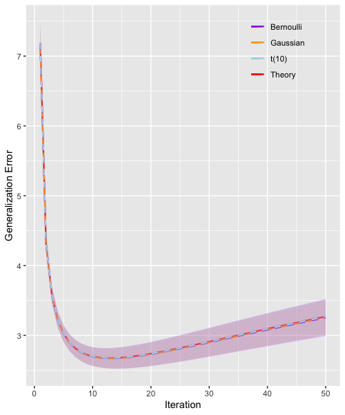
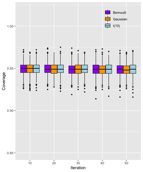
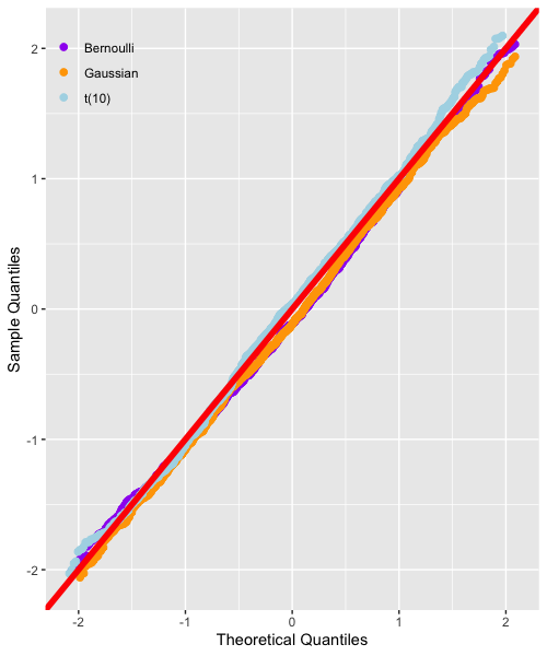
Figure 1. Linear regression model with squared loss. Simulation parameters: $\eta=0.3$, $m=1200$, $n=1000$, $\mu_{\ast}\in\mathbb{R}^{n}$ are i.i.d. $\lvert\mathcal{N}(0,5)\rvert$, $\xi\in\mathbb{R}^{m}$ are i.i.d. $\mathcal{N}(0,1)$, $\sqrt{n}A$ has i.i.d. entries following $\mathcal{N}(0,1)$ (orange), $t$ distribution with $10$ degrees of freedom (blue), Bernoulli$(1/2)$ (purple), with proper normalization in the latter two cases so that the variance is $1$. The algorithm is run for $50$ iterations with Monte Carlo repetition $B=1000$.

We report some illustrative simulation results for the linear regression model with squared loss and no regularizer in Figure 1:

• The left panel of Figure 1 compares the generalization error estimator $\widehat{\mathscr{E}}_{\lvert\cdot\rvert^{2}}^{(t)}$ with the theoretical generalization error $\mathscr{E}_{\lvert\cdot\rvert^{2}}^{(t)}$ for both Gaussian and non-Gaussian designs, showing excellent agreement in both cases. Notably, the generalization error reaches its minimum around iteration 12 in our simulation setup, showing that early stopping of gradient descent may improve generalization performance, cf. [AKT19, ADT20, BT24].

• Using $\widehat{\sigma}^{(t)}_{\mathrm{db}}$ computed from (3.10), the middle panel displays the coverage of $95\%$ CIs for all coordinates. For all design distributions, the proposed CIs in (4.4) achieve approximate nominal coverage.

• The right panel validates the distributional characterization of $\widehat{\mu}^{(t)}_{\mathrm{db}}$. Since the bias and the variance are identical across coordinates, we report only the QQ-plot of $(\widehat{\mu}^{(t)}_{\mathrm{db};1}-\mu_{\ast;1})/\widehat{\sigma}^{(t)}_{\mathrm{db}}$ at the last iteration of our simulation. The empirical quantiles align closely with the theoretical standard Gaussian quantiles, supporting the conclusion that $\widehat{\mu}^{(t)}_{\mathrm{db}}\stackrel{{\scriptstyle d}}{{\approx}}\mu_{\ast}+\sigma^{(t)}_{\mathrm{db}}\cdot\mathsf{Z}$.

Strictly speaking, our theory does not apply to $t(10)$ due to its heavy tails. However, the simulation results presented in these plots suggest that the moment condition in (A2) could potentially be further relaxed for our theory to hold.

In Appendix C, we provide additional simulation results where the squared loss is replaced by a robust loss tailored to handle heavy-tailed errors. The simulation results, shown in Figure 3, exhibit patterns similar to those in Figure 1 and remain consistent across a wide range of simulation parameters (additional figures are omitted for brevity).

5. Example II: Generalized logistic regression

Suppose we observe $(Y_{i},A_{i})\in\{\pm 1\}\times\mathbb{R}^{n}$ according to the model

$$Y_{i}=\operatorname{\texttt{sgn}}\big{(}\langle A_{i},\mu_{\ast}\rangle+\xi_{i}\big{)},\quad i\in[m].$$ (5.1)

Here for definiteness, we interpret $\operatorname{\texttt{sgn}}(x)=2\cdot\bm{1}_{x\geq 0}-1$ for $x\in\mathbb{R}$. The above model is also known under the name of the noisy one-bit compressed sensing model, and can be recast into (1.1) by setting $\mathcal{F}(z,\xi)=\operatorname{\texttt{sgn}}(z+\xi)$.

Consider a loss function $\mathsf{L}(x,y)$ that does not depend on the iteration, and the associated proximal gradient descent algorithm with a fixed step size $\eta>0$:

$$\mu^{(t)}=\operatorname{\mathsf{prox}}_{\eta\mathsf{f}}\big{(}\mu^{(t-1)}-\eta\cdot A^{\top}\partial_{1}\mathsf{L}(A\mu^{(t-1)},Y)\big{)}.$$ (5.2)

5.1. Relation to logistic regression

Let $\rho(t)=\log(1+e^{t})$ and therefore $\rho^{\prime}(t)=1/(1+e^{-t})$, $\rho^{\prime}(-t)=1/(1+e^{t})$. In logistic regression, we observe i.i.d. data $(\widetilde{Y}_{i},A_{i})\in\{0,1\}\times\mathbb{R}^{n}$ generated according to the model

$$\operatorname{\mathbb{P}}\big{(}\widetilde{Y}_{i}=1|A_{i}\big{)}=1/(1+e^{-\langle A_{i},\mu_{\ast}\rangle})=\rho^{\prime}(\langle A_{i},\mu_{\ast}\rangle),\quad i\in[m].$$

The maximum likelihood estimator $\widehat{\mu}^{\mathrm{MLE}}$ solves

$$\widehat{\mu}^{\mathrm{MLE}}\in\operatorname*{arg\,min\,}_{\mu\in\mathbb{R}^{n}}-\sum_{i\in[m]}\Big{\{}\widetilde{Y}_{i}\cdot\log\rho^{\prime}(\langle A_{i},\mu_{\ast}\rangle)+(1-\widetilde{Y}_{i})\cdot\log\rho^{\prime}(-\langle A_{i},\mu_{\ast}\rangle)\Big{\}}.$$

It is natural to run gradient descent for the loss function above.

To setup its equivalence to (5.1), consider the reparametrization $Y_{i}\equiv 2\widetilde{Y}_{i}-1$. Then it is easy to verify that $\{(Y_{i},A_{i})\}_{i\in[m]}$ are i.i.d. observations from the model (5.1) with the errors $\{\xi_{i}\}$ being i.i.d. random variables with c.d.f. $\operatorname{\mathbb{P}}(\xi_{1}\leq t)=1/(1+e^{-t})=\rho^{\prime}(t)$. Moreover,

$$\widehat{\mu}^{\mathrm{MLE}}\in\operatorname*{arg\,min\,}_{\mu\in\mathbb{R}^{n}}\sum_{i\in[m]}\log\big{(}1+e^{-Y_{i}\cdot\langle A_{i},\mu\rangle}\big{)}=\operatorname*{arg\,min\,}_{\mu\in\mathbb{R}^{n}}\sum_{i\in[m]}\rho\big{(}-Y_{i}\cdot\langle A_{i},\mu\rangle\big{)}.$$

In other words, by setting the loss function as $\mathsf{L}(x,y)\equiv\rho(-yx)$, $\widehat{\mu}^{\mathrm{MLE}}$ is stationary point to the gradient descent algorithm

$$\mu^{(t)} \equiv\mu^{(t-1)}-\eta\cdot A^{\top}\partial_{1}\mathsf{L}(A\mu^{(t-1)},Y).$$

With this identification, it suffices to work with the model (5.1) with a general loss function $\mathsf{L}(x,y)$.

5.2. Distributional characterizations

Since $\Upsilon_{t}(\mathfrak{z}^{[0:t]})$ is non-differentiable with respect to $\mathfrak{z}^{(0)}$, the regularity conditions (A5’) in Theorem 2.3 and (A5*) in Theorem 3.1 are not satisfied. However, with a non-trivial smoothing technique, these distributional results continue to hold.

Theorem 5.1.

Suppose Assumption A and (A4*) hold for some $K,\Lambda\geq 2$, and the loss function $\mathsf{L}$ satisfies

$$\lvert\partial_{1}\mathsf{L}(0,0)\rvert+\sup_{x\in\mathbb{R},y\in[-1,1]}\max_{{\alpha}=2,3}\lvert\partial_{\alpha}\mathsf{L}(x,y)\rvert\leq\Lambda.$$ (5.3)

1. For a sequence of $\Lambda_{\psi}$-pseudo-Lipschitz functions $\{\psi_{k}:\mathbb{R}^{2t+1}\to\mathbb{R}\}_{k\in[m\vee n]}$ of order 2 where $\Lambda_{\psi}\geq 2$, the averaged distributional characterizations in Theorem 2.3 hold for the gradient descent iterates in (5.2), with an error bound $\big{(}K\Lambda\Lambda_{\psi}L_{\mu}(1\wedge\sigma_{\mu_{\ast}})^{-1}\big{)}^{c_{t}}\cdot n^{-1/c_{t}}$.

2. Theorem 3.1 holds for the output $(\widehat{\bm{\tau}}^{[t]},\widehat{\bm{\rho}}^{[t]})$ in Algorithm 1 using gradient descent iterates in (5.2), with an error bound $\big{(}K\Lambda L_{\mu}(1\wedge\sigma_{\mu_{\ast}})^{-1}\big{)}^{c_{t}}\cdot n^{-1/c_{t}}$.

It is easy to verify that the loss function $\mathsf{L}(x,y)\equiv\rho(-yx)$ used in logistic regression satisfies (5.3) (details may be found in Section 9.5). Moreover, for random noises $\{\xi_{i}\}$’s, the above theorem holds for every realization of these noises.

At a high level, the smoothing technique used in the proof of Theorem 5.1 proceeds as follows. We construct a sequence of smooth approximation functions $\{\varphi_{\varepsilon}\}_{\varepsilon>0}$ such that $\varphi_{\varepsilon}\to\operatorname{\texttt{sgn}}$ as $\varepsilon\to 0$ in a suitable sense. Then for each $\varepsilon>0$, we may compute the state evolution parameters $\texttt{SE}_{\varepsilon}^{(t)}$ associated with the smoothed model according to Definition 2.1. We also construct ‘smoothed data’ $\{Y_{\varepsilon;i}\equiv\varphi_{\varepsilon}(\langle A_{i},\mu_{\ast}\rangle+\xi_{i})\}_{i\in[m]}$, and compute ‘smoothed gradient descent’ $\mu^{(t)}_{\varepsilon}$ according to (2.1). Since our theory applies to $\mu^{(t)}_{\varepsilon}$ via $\texttt{SE}_{\varepsilon}^{(t)}$ for any $\varepsilon>0$, the key task is to prove that these quantities remain stable as $\varepsilon\to 0$. We will prove such stability estimates for $\texttt{SE}_{\varepsilon}^{(t)}$ in Lemma 9.2, and for $\mu^{(t)}_{\varepsilon}$ in Lemma 9.4.

Interestingly, the smoothing technique also provides a method to compute the information parameter $\delta_{t}$ via the limit of ‘smoothed information parameter’ $\delta_{\varepsilon;t}$ in Lemma 5.2, as well as the bias parameter $b^{(t)}_{\mathrm{db}}$ in Proposition 5.4 below.

5.3. The information parameter

Due to the non-differentiability issue of $\Upsilon_{t}$, it is understood that $\delta_{t}$ is defined in the sense of Gaussian integration-by-parts formula in (2.10), whenever well-defined.

To state our formula for $\delta_{t}$, we need the some further notation. For a general loss function $\mathsf{L}$, let $\Theta_{t}^{\circ}:\mathbb{R}^{[0:t]}\to\mathbb{R}$ be defined recursively via the relation

$$\Theta_{t}^{\circ}(z_{[0:t]})\equiv z_{t}-\sum_{s\in[1:t-1]}\eta_{s-1}\rho_{t-1,s}\cdot\partial_{1}\mathsf{L}\big{(}\Theta^{\circ}_{s}(z_{[0:s]}),z_{0}\big{)}.$$ (5.4)

For $v>0$, let $\mathfrak{g}_{v}$ be the Lebesgue density of $\mathcal{N}(0,v^{2})$.

Lemma 5.2.

Suppose (A1), (A3) and (A4*), and (5.3) hold. Then with $(\mathsf{Z}_{0},\mathsf{Z}_{[1:t]})\sim\mathcal{N}\big{(}0,\operatorname{Var}\big{(}\operatorname{\mathbb{E}}^{(0)}\big{[}\mathfrak{Z}^{([0:t])}|\mathfrak{Z}^{([1:t])}\big{]}\big{)}\big{)}$, if $\mathfrak{v}_{t}\equiv\operatorname{\mathbb{E}}^{(0)}\operatorname{Var}(\mathfrak{Z}^{(0)}|\mathfrak{Z}^{([1:t])})>0$,

$$\delta_{t} =-2\phi\eta\cdot\operatorname{\mathbb{E}}^{(0)}\Big{\{}\mathfrak{g}_{\mathfrak{v}_{t}}(\xi_{\pi_{m}}+\mathsf{Z}_{0})\cdot e_{t}^{\top}\big{(}I_{t}+\eta\cdot\mathfrak{L}_{1}(U,\mathsf{Z}_{[1:t]})\mathfrak{O}_{t}(\bm{\rho}^{[t-1]})\big{)}^{-1}\mathfrak{l}_{2}(U,\mathsf{Z}_{[1:t]})\Big{\}}.$$

Here $U\sim\mathrm{Unif}[-1,1]$ is independent of all other variables, and

• $\mathfrak{L}_{1}(U,\mathsf{Z}_{[1:t]})\equiv\mathrm{diag}\big{(}\big{\{}\partial_{11}\mathsf{L}\big{(}\Theta_{t}^{\circ}(U,\mathsf{Z}_{[1:s]}),U\big{)}\}_{s\in[t]}\big{)}\in\mathbb{R}^{t\times t}$,

• $\mathfrak{l}_{2}(U,\mathsf{Z}_{[1:t]})\equiv\big{(}\partial_{12}\mathsf{L}(\Theta_{t}^{\circ}(U,\mathsf{Z}_{[1:s]}),U)\big{)}_{s\in[t]}\in\mathbb{R}^{t}$.

For squared loss $\mathsf{L}(x,y)=(x-y)^{2}/2$, we have $\delta_{t}=-2\operatorname{\mathbb{E}}^{(0)}\mathfrak{g}_{\sigma_{\mu_{\ast}}}(\xi_{\pi_{m}})\cdot\sum_{s\in[1:t]}\tau_{t,s}$, provided that $\mu_{\ast}\neq 0$.

Under the squared loss, the complicated formula of $\delta_{t}$ simplifies significantly, revealing a structure reminiscent of the linear regression case (cf. Lemma 4.2). While the squared loss may not initially appear as a natural choice for the model (5.1), [HJLZ18] showed that the global least squares estimator (the convergent point of $\mu^{(t)})$ achieves a near rate-optimal convergence rate for a scaled $\mu_{\ast}$ in the low dimensional case $m\ll n$ under Gaussian noise.

5.4. Mean-field statistical inference

5.4.1. Estimation of generalization error

Consider the generalization error (3.1) under the loss function $\mathsf{H}(x,y)$. The generalization error estimator $\widehat{\mathscr{E}}_{\mathsf{H}}^{(t)}$ takes the form as in (3.2). Its validity in the following proposition is formally justified by a smoothing argument similar to that of Theorem 5.1.

Proposition 5.3.

Assume the same conditions as in Theorem 5.1-(1). Suppose that $\mathsf{H}\in C^{3}(\mathbb{R}^{2})$ has mixed derivatives of order 3 all bounded by $\Lambda$. Then for any $q\in\mathbb{N}$, there exists some $c_{t}=c_{t}(t,q)>1$ such that

$$\operatorname{\mathbb{E}}^{(0)}\lvert\widehat{\mathscr{E}}_{\mathsf{H}}^{(t)}-\mathscr{E}_{\mathsf{H}}^{(t)}(A,Y)\rvert^{q}\leq\big{(}K\Lambda L_{\mu}(1\wedge\sigma_{\mu_{\ast}})^{-1}\big{)}^{c_{t}}\cdot n^{-1/c_{1}}.$$

As the logistic loss $\mathsf{L}(x,y)=\log(1+e^{-xy})$ satisfies (5.3), the above proposition holds for $\mathsf{H}=\mathsf{L}$ in logistic regression.

5.4.2. Debiased gradient descent inference

Consider the oracle debiased gradient descent iterate $\mu^{(t)}_{\mathrm{db}}$ or its data-driven version $\widehat{\mu}^{(t)}_{\mathrm{db}}$ taking the form (3.9).

To state our result, recall $\bm{\delta}^{[t]}\equiv(\delta_{s})_{s\in[1:t]}$ given by Lemma 5.2. Let $\bm{\omega}^{[t]}\equiv(\bm{\tau}^{[t]})^{-1}$, where with $\bm{L}_{11;k}^{[t]}(z_{[0:t]})\equiv\mathrm{diag}\big{(}\big{\{}\partial_{11}\mathsf{L}(\Theta_{s;k}(z_{[0:t]}),\operatorname{\texttt{sgn}}(z_{0}+\xi_{k}))\big{\}}_{s\in[1:t]}\big{)}$,

$$\bm{\tau}^{[t]}\equiv-\phi\eta\cdot\operatorname{\mathbb{E}}^{(0)}\big{(}I_{t}+\eta\cdot\bm{L}_{11;\pi_{m}}^{[t]}(\mathfrak{Z}^{([0:t])})\mathfrak{O}_{t}(\bm{\rho}^{[t-1]})\big{)}^{-1}\bm{L}_{11;\pi_{m}}^{[t]}(\mathfrak{Z}^{([0:t])}).$$ (5.5)

Let the bias $b^{(t)}_{\mathrm{db}}\equiv-\langle\bm{\omega}^{[t]}\bm{\delta}^{[t]},e_{t}\rangle$, and the variance $(\sigma^{(t)}_{\mathrm{db}})^{2}\equiv\bm{\omega}_{t\cdot}^{[t]}\Sigma_{\mathfrak{W}}^{[t]}\bm{\omega}_{t\cdot}^{[t],\top}$.

Proposition 5.4.

Suppose Assumption A and (A4*), and (5.3) hold.

1. For a sequence of $\Lambda_{\psi}$-pseudo-Lipschitz functions $\{\psi_{\ell}:\mathbb{R}\to\mathbb{R}\}_{\ell\in[n]}$ of order 2 where $\Lambda_{\psi}\geq 2$, the averaged distributional characterizations for $\mu^{(t)}_{\mathrm{db}}$ in Theorem 3.4-(2) hold with $b^{(t)}_{\mathrm{db}},\sigma^{(t)}_{\mathrm{db}}$ specified as above, and with an error bound $\big{(}K\Lambda\Lambda_{\psi}L_{\mu}(1\wedge\sigma_{\mu_{\ast}})^{-1}(1\wedge\tau_{\ast}^{(t)})^{-1}\big{)}^{c_{t}}\cdot n^{-1/c_{t}}$.

2. For the squared loss $\mathsf{L}(x,y)=(x-y)^{2}/2$, if $\sigma_{\mu_{\ast}}>0$,

   $$b^{(t)}_{\mathrm{db}}=2\operatorname{\mathbb{E}}^{(0)}\mathfrak{g}_{\sigma_{\mu_{\ast}}}(\xi_{\pi_{m}}),\,(\sigma^{(t)}_{\mathrm{db}})^{2}=\phi^{-1}\operatorname{\mathbb{E}}^{(0)}\big{(}\mathfrak{Z}^{(t)}-\operatorname{\texttt{sgn}}(\mathfrak{Z}^{(0)}+\xi_{\pi_{m}})\big{)}^{2}.$$

In logistic regression, the generic proposal (3.11) can be used to estimate the bias parameter $b^{(t)}_{\mathrm{db}}$. Estimating the signal strength $\sigma_{\mu_{\ast}}$ in mean-field logistic regression is a non-trivial and separate problem; several notable methods include the ProbeFrontier method developed in [SC19, Section 3.1] and the SLOE method developed in [YYMD21]. However, estimation of $\sigma_{\mu_{\ast}}$ is unnecessary when the parameter of interest is $\mu_{\ast}/\lVert\mu_{\ast}\rVert$ as in the single-index model [Bel22]. On the other hand, the variance parameter $(\sigma^{(t)}_{\mathrm{db}})^{2}$ can be estimated using the generic proposal (3.10). Under the squared loss, it can also be estimated simply by the rescaled generalization error estimate $\phi^{-1}\widehat{\mathscr{E}}_{\lvert\cdot\rvert^{2}}^{(t-1)}$ as in the linear regression.

5.4.3. Some simulations

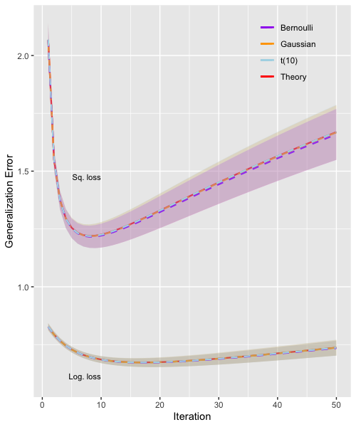
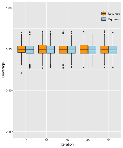
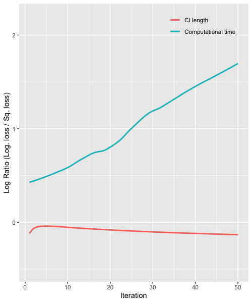
Figure 2. Logistic regression model with squared/logistic loss. Simulation parameters: $\eta=0.5$, $m=1200$, $n=1000$, $\mu_{\ast}\in\mathbb{R}^{n}$ are i.i.d. $\lvert\mathcal{N}(0,5)\rvert$. For the generalization error plot (left panel), $\sqrt{n}A$ has i.i.d. entries following $\mathcal{N}(0,1)$ (orange), $t$ distribution with $10$ degrees of freedom (blue), Bernoulli$(1/2)$ (purple), with proper normalization in the latter two cases so that the variance is $1$. The other two plots (middle and right panels) show simulation results under the Gaussian setting only. The algorithm is run for $50$ iterations with Monte Carlo repetition $B=1000$.

We report in Figure 2 some simulation results under both the squared and logistic losses for logistic regression without regularization:

• The left panel demonstrates that the early stopping phenomenon observed for gradient descent in Figure 1 also holds in logistic regression for both loss functions.

• The middle panel shows that the CI’s constructed using both loss functions achieve the nominal coverage level, with comparable coverage performance.

• The right panel shows the logarithm (base 10) of the ratio

  $$\log_{10}\frac{@\text{ under logistic loss}}{@\text{ under squared loss}},$$

  defined for $@\in\{\text{CI length},\text{Computational time}\}$. This plot highlights two interesting observations: (i) the CI lengths under both losses are comparable, and (ii) the squared loss offers significant computational advantages over the logistic loss. Specifically, in Algorithm 1, $\widehat{\bm{\tau}}^{[t]}$ can be computed in a single step under the squared loss, whereas all $\{\widehat{\bm{\tau}}^{[t]}_{k}\}_{k\in[m]}$ need be computed under the logistic loss. This advantage becomes increasingly pronounced with more iterations; for instance, by iteration 50, computation under the logistic loss is approximately 50 times slower in our simulation setup.

Our simulations are conducted with known signal strength $\sigma_{\mu_{\ast}}$ to illustrate the numerical features inherent to our inference methods. As mentioned earlier, estimating $\sigma_{\mu_{\ast}}$ is a separate problem, and can be tackled by existing methods such as ProbeFrontier [SC19] and SLOE [YYMD21]. Furthermore, while the latter two plots in Figure 2 display results under Gaussian designs $A$, the findings remain nearly identical for non-Gaussian designs, such as Bernoulli or $t(10)$ variables (as used in Figure 1 in linear regression). For brevity, we omit these additional plots.

In Appendix C, we examine the numerical performance of our proposed inference method when the errors $\{\xi_{i}\}$’s are i.i.d. standard Gaussian as in [HJLZ18]. In this setting, it is easy to construct a closed-form estimator for $\sigma_{\mu_{\ast}}$ (see Eqn. (C.1) for details). The simulation results, reported in Figure 4 therein, exhibit qualitatively similar patterns to those observed in Figure 1.

6. Proofs for Section 2

6.1. An apriori estimate

The following apriori estimates are important for the proofs of many results in the sequel. Moreover, the calculations in the proof of these estimates provide the precise formulae that lead to Algorithm 1.

Lemma 6.1.

Suppose (A1), (A3), (A4’) and (A5’) hold. The following hold for some $c_{t}=c_{t}(t)>1$:

1. $\lVert\bm{\tau}^{[t]}\rVert_{\operatorname{op}}+\lVert\bm{\rho}^{[t]}\rVert_{\operatorname{op}}\leq(K\Lambda)^{c_{t}}$.

2. $\lVert\Sigma_{\mathfrak{Z}}^{[t]}\rVert_{\operatorname{op}}+\lVert\Sigma_{\mathfrak{W}}^{[t]}\rVert_{\operatorname{op}}+\lVert\bm{\delta}^{[t]}\rVert\leq(K\Lambda L_{\mu})^{c_{t}}$.

3. $\max\limits_{k\in[m],r\in[1:t]}\big{(}\lvert\Upsilon_{r;k}(z^{([0:r])})\rvert+\lvert\Theta_{r;k}(z^{([0:r])})\rvert\big{)}\leq(K\Lambda)^{c_{t}}\cdot\big{(}1+\lVert z^{([0:t])}\rVert\big{)}$.

4. $\max\limits_{\ell\in[n],r\in[1:t]}\lvert\Omega_{r;\ell}(w^{([1:r])})\rvert\leq(K\Lambda L_{\mu})^{c_{t}}\cdot\big{(}1+\lVert w^{([1:t])}\rVert\big{)}$.

5. $\max\limits_{\begin{subarray}{c}k\in[m],\ell\in[n],r,s\in[1:t]\end{subarray}}\big{(}\lvert\partial_{(s)}\Upsilon_{r;k}(z^{([0:r])})\rvert+\lvert\partial_{(s)}\Omega_{r;\ell}(w^{([1:r])})\rvert\big{)}\leq(K\Lambda)^{c_{t}}.$

Proof.

The proof is divided into several steps.

(Step 1). We prove the estimate in (1) in this step. First, for any $k\in[m]$ and $1\leq s\leq t$, using (S1),

$$\partial_{(s)}\Upsilon_{t;k}(z^{([0:t])}) \equiv-\eta_{t-1}\partial_{11}\mathsf{L}_{t-1}\big{(}\Theta_{t;k}(z^{([0:t])}),\mathcal{F}(z^{(0)},\xi_{k})\big{)}$$

$$\qquad\times\bigg{(}\bm{1}_{t=s}+\sum_{r\in[1:t-1]}\rho_{t-1,r}\partial_{(s)}\Upsilon_{r;k}(z^{([0:r])})\bigg{)}.$$

In matrix form, with $\bm{\Upsilon}_{k}^{{}^{\prime};[t]}(z^{([0:t])})\equiv\big{(}\partial_{(s)}\Upsilon_{r;k}(z^{([0:r])})\big{)}_{r,s\in[1:t]}$ and $\bm{L}^{[t]}_{k}(z^{([0:t])})\equiv\mathrm{diag}\big{(}\big{\{}-\eta_{s-1}\partial_{11}\mathsf{L}_{s-1}\big{(}\Theta_{s;k}(z^{([0:s])}),\mathcal{F}(z^{(0)},\xi_{k})\big{)}\big{\}}_{s\in[1:t]}\big{)}$,

$$\bm{\Upsilon}_{k}^{{}^{\prime};[t]}(z^{([0:t])})=\bm{L}^{[t]}_{k}(z^{([0:t])})+\bm{L}^{[t]}_{k}(z^{([0:t])})\mathfrak{O}_{t}(\bm{\rho}^{[t-1]})\bm{\Upsilon}_{k}^{{}^{\prime};[t]}(z^{([0:t])}).$$

Solving for $\bm{\Upsilon}_{k}^{{}^{\prime};[t]}$ yields that

$$\bm{\Upsilon}_{k}^{{}^{\prime};[t]}(z^{([0:t])})=\big{[}I_{t}-\bm{L}^{[t]}_{k}(z^{([0:t])})\mathfrak{O}_{t}(\bm{\rho}^{[t-1]})\big{]}^{-1}\bm{L}^{[t]}_{k}(z^{([0:t])}).$$ (6.1)

As $\bm{L}^{[t]}_{k}(z^{([0:t])})\mathfrak{O}_{t}(\bm{\rho}^{[t-1]})$ is a lower triangular matrix with $0$ diagonal elements, $\big{(}\bm{L}^{[t]}_{k}(z^{([0:t])})\mathfrak{O}_{t}(\bm{\rho}^{[t-1]})\big{)}^{t}=0_{t\times t}$, and therefore using $\lVert\bm{L}^{[t]}_{k}(z^{([0:t])})\rVert_{\operatorname{op}}\leq\Lambda^{2}$,

$$\lVert\bm{\Upsilon}_{k}^{{}^{\prime};[t]}(z^{([0:t])})\rVert_{\operatorname{op}} \leq\bigg{(}1+\sum_{r\in[1:t]}\Lambda^{2r}\lVert\bm{\rho}^{[t-1]}\rVert_{\operatorname{op}}^{r}\bigg{)}\cdot\Lambda^{2}\leq\Lambda^{c_{0}t}\cdot\lVert\bm{\rho}^{[t-1]}\rVert_{\operatorname{op}}^{t}.$$ (6.2)

Using definition of $\{\tau_{r,s}\}$, we then arrive at

$$\lVert\bm{\tau}^{[t]}\rVert_{\operatorname{op}}\leq(K\Lambda)^{c_{0}t}\cdot\lVert\bm{\rho}^{[t-1]}\rVert_{\operatorname{op}}^{t}.$$ (6.3)

Next, for any $\ell\in[n]$ and $1\leq s\leq t$, using (S3),

$$\partial_{(s)}\Omega_{t;\ell}(w^{([1:t])}) =\mathsf{P}_{t;\ell}^{\prime}\big{(}\Delta_{t;\ell}(w^{([1:t])})\big{)}$$

$$\quad\times\bigg{(}\bm{1}_{t=s}+\sum_{r\in[1:t]}(\tau_{t,r}+\bm{1}_{t=r})\cdot\partial_{(s)}\Omega_{r-1;\ell}(w^{([1:r-1])})\bigg{)}.$$

In matrix form, with $\bm{\Omega}_{\ell}^{{}^{\prime};[t]}(w^{([1:t])})\equiv\big{(}\partial_{(s)}\Omega_{r;\ell}(w^{([1:r])})\big{)}_{r,s\in[1:t]}$ and $\bm{P}^{[t]}_{\ell}(w^{([1:t])})\equiv\mathrm{diag}\big{(}\big{\{}\mathsf{P}_{s;\ell}^{\prime}(\Delta_{s;\ell}(w^{([1:t])}))\big{\}}_{s\in[1:t]}\big{)}$,

$$\bm{\Omega}_{\ell}^{{}^{\prime};[t]}(w^{([1:t])})=\bm{P}^{[t]}_{\ell}(w^{([1:t])})\big{[}I_{t}+(\bm{\tau}^{[t]}+I_{t})\mathfrak{O}_{t}\big{(}\bm{\Omega}_{\ell}^{{}^{\prime};(t-1)}(w^{([1:t-1])})\big{)}\big{]}.$$ (6.4)

Consequently,

$$\lVert\bm{\Omega}_{\ell}^{{}^{\prime};[t]}(w^{([1:t])})\rVert_{\operatorname{op}}\leq\Lambda\cdot\Big{(}1+(1+\lVert\bm{\tau}^{[t]}\rVert_{\operatorname{op}})\cdot\lVert\bm{\Omega}_{\ell}^{{}^{\prime};(t-1)}(w^{([1:t-1])})\rVert_{\operatorname{op}}\Big{)}.$$

Iterating the bound and using the trivial initial condition $\lVert\bm{\Omega}_{\ell}^{{}^{\prime};(1)}(w^{(1)})\rVert_{\operatorname{op}}\leq\Lambda$,

$$\lVert\bm{\Omega}_{\ell}^{{}^{\prime};[t]}(w^{([1:t])})\rVert_{\operatorname{op}}\leq\big{(}\Lambda(1+\lVert\bm{\tau}^{[t]}\rVert_{\operatorname{op}})\big{)}^{c_{t}}.$$ (6.5)

Using the definition of $\{\rho_{r,s}\}$, we then have

$$\lVert\bm{\rho}^{[t]}\rVert_{\operatorname{op}}\leq\big{(}\Lambda(1+\lVert\bm{\tau}^{[t]}\rVert_{\operatorname{op}})\big{)}^{c_{t}}.$$ (6.6)

Combining (6.3) and (6.6), it follows that

$$\lVert\bm{\tau}^{[t]}\rVert_{\operatorname{op}}\leq(K\Lambda)^{c_{t}}\cdot(1+\lVert\bm{\tau}^{[t-1]}\rVert_{\operatorname{op}})^{c_{t}}.$$

Iterating the bound and using the initial condition $\lVert\bm{\tau}^{[1]}\rVert_{\operatorname{op}}\leq\Lambda^{2}$ to conclude the bound for $\lVert\bm{\tau}^{[t]}\rVert_{\operatorname{op}}$. The bound for $\lVert\bm{\rho}^{[t]}\rVert_{\operatorname{op}}$ then follows from (6.6).

(Step 2). In this step we note the following recursive estimates:

1. A direct induction argument for (S1) shows that

   $$\max_{k\in[m]}\max_{r\in[1:t]}\lvert\Upsilon_{r;k}(z^{([0:r])})\rvert\leq(K\Lambda)^{c_{t}}\cdot\big{(}1+\lVert z^{([0:t])}\rVert\big{)}.$$

2. A direct induction argument for (S3) shows that

   $$\max_{\ell\in[n]}\max_{r\in[1:t]}\lvert\Omega_{r;\ell}(w^{([1:r])})\rvert \leq(K\Lambda L_{\mu})^{c_{t}}\cdot\big{(}1+\lVert w^{([1:t])}\rVert+\lVert\bm{\delta}^{[t]}\rVert\big{)}.$$

3. Using (S2), we have

   $$\lVert\Sigma_{\mathfrak{Z}}^{[t]}\rVert_{\operatorname{op}} \leq(K\Lambda L_{\mu})^{c_{t}}\cdot\big{(}1+\lVert\Sigma_{\mathfrak{W}}^{[t-1]}\rVert_{\operatorname{op}}+\lVert\bm{\delta}^{[t-1]}\rVert\big{)},$$

   $$\lVert\Sigma_{\mathfrak{W}}^{[t]}\rVert_{\operatorname{op}} \leq(K\Lambda)^{c_{t}}\cdot\big{(}1+\lVert\Sigma_{\mathfrak{Z}}^{[t]}\rVert_{\operatorname{op}}\big{)}.$$

(Step 3). In order to use the recursive estimates in Step 2, in this step we prove the estimate for $\lVert\bm{\delta}^{[t]}\rVert$. For $k\in[m]$, let $\mathsf{L}_{t-1;k}^{\mathcal{F}}(u_{1},u_{2})\equiv\mathsf{L}_{t-1;k}(u_{1},\mathcal{F}(u_{2},\xi_{k}))$. Then by assumption, the mapping $(u_{1},u_{2})\mapsto\partial_{1}\mathsf{L}_{t-1;k}^{\mathcal{F}}(u_{1},u_{2})$ is $\Lambda$-Lipschitz on $\mathbb{R}^{2}$. By using (S1), we then have

$$\lvert\partial_{(0)}\Upsilon_{t;k}(z^{([0:t])})\rvert =\bigg{\lvert}-\eta_{t-1}\partial_{11}\mathsf{L}_{t-1}^{\mathcal{F}}\big{(}\Theta_{t;k}(z^{([0:t])}),z^{(0)})\big{)}\cdot\bigg{(}\sum_{r\in[1:t-1]}\rho_{t-1,r}\partial_{(0)}\Upsilon_{r;k}(z^{([0:r])})\bigg{)}$$

$$\qquad-\eta_{t-1}\partial_{12}\mathsf{L}_{t-1}^{\mathcal{F}}\big{(}\Theta_{t;k}(z^{([0:t])}),z^{(0)})\big{)}\bigg{\rvert}$$

$$\leq t\Lambda^{2}\cdot\lVert\bm{\rho}^{[t-1]}\rVert_{\operatorname{op}}\cdot\max_{r\in[1:t-1]}\lvert\partial_{(0)}\Upsilon_{r;k}(z^{([0:r])})\rvert.$$

Invoking the proven estimate in (1) and iterating the above bound with the trivial initial condition $\lvert\partial_{(0)}\Upsilon_{1;k}(z^{([0:1])})\rvert\leq\Lambda^{2}$ to conclude that $\lvert\partial_{(0)}\Upsilon_{t;k}(z^{([0:t])})\rvert\leq(K\Lambda)^{c_{t}}$, and therefore by definition of $\delta_{t}$, we conclude that

$$\lVert\bm{\delta}^{[t]}\rVert\leq(K\Lambda)^{c_{t}}.$$ (6.7)

(Step 4). Now we shall use the estimate for $\lVert\bm{\delta}^{[t]}\rVert$ in Step 3 to run the recursive estimates in Step 2. Combining the first line of (c) and (6.7), we have

$$\lVert\Sigma_{\mathfrak{Z}}^{[t]}\rVert_{\operatorname{op}} \leq(K\Lambda L_{\mu})^{c_{t}}\cdot\big{(}1+\lVert\Sigma_{\mathfrak{W}}^{[t-1]}\rVert_{\operatorname{op}}\big{)}.$$

Combined with the second line of (c), we obtain

$$\lVert\Sigma_{\mathfrak{Z}}^{[t]}\rVert_{\operatorname{op}} \leq(K\Lambda L_{\mu})^{c_{t}}\cdot\Big{(}1+\max_{r\in[1:t-1]}\lVert\Sigma_{\mathfrak{Z}}^{[r]}\rVert_{\operatorname{op}}\Big{)}.$$

Coupled with the initial condition $\lVert\Sigma_{\mathfrak{Z}}^{[1]}\rVert_{\operatorname{op}}\leq L_{\mu}^{2}$, we arrive at the estimate

$$\lVert\Sigma_{\mathfrak{Z}}^{[t]}\rVert_{\operatorname{op}}+\lVert\Sigma_{\mathfrak{W}}^{[t]}\rVert_{\operatorname{op}}+\lVert\bm{\delta}^{[t]}\rVert\leq(K\Lambda L_{\mu})^{c_{t}}.$$

The proof of (1)-(4) is complete by collecting the estimates. The estimate in (5) follows by combining (6.2) and (6.5) along with the estimate in (1). ∎

6.2. Proofs of Theorems 2.2 and 2.3

The proofs of Theorems 2.2 and 2.3 rely on the general state evolution theory developed in [Han24]. For the convenience of the reader, we review some of its basics in Appendix A.

Proof of Theorem 2.2.

The proof is divided into several steps.

(Step 1). Let us now rewrite the proximal gradient descent algorithm (2.1) into the canonical form in which the state evolution theory in [Han24] can be applied. Consider initialization $u^{(-1)}=0_{m}$, $v^{(-1)}=\mu_{\ast}$ at iteration $t=-1$. For $t=0$, let $u^{(0)}\equiv Av^{(-1)}=A\mu_{\ast}$, $v^{(0)}\equiv\mu^{(0)}$. For $t\geq 1$,

$$u^{(t)} \equiv A\mathsf{R}_{t-1}(v^{(t-1)})\in\mathbb{R}^{m},$$

$$v^{(t)} \equiv\mathsf{R}_{t-1}(v^{(t-1)})-\eta_{t-1}\cdot A^{\top}\partial_{1}\mathsf{L}_{t-1}\big{(}u^{(t)},\mathcal{F}(u^{(0)},\xi)\big{)}\in\mathbb{R}^{n}.$$

Here $\mathsf{R}_{t-1}\equiv\mathsf{P}_{t-1}\cdot\bm{1}_{t\geq 2}+\mathrm{id}\cdot\bm{1}_{t=1}$. The proximal gradient descent is identified as $\mu^{(t)}=\mathsf{R}_{t}(v^{(t)})$ for $t\geq 0$. Consequently, for $t\geq 0$,

$$\mathsf{F}_{t}^{\langle 1\rangle}(v^{([-1:t-1])}) =\mathsf{R}_{t-1}(v^{(t-1)})\bm{1}_{t\geq 1}+\mu_{\ast}\bm{1}_{t=0},$$

$$\mathsf{F}_{t}^{\langle 2\rangle}(v^{([-1:t-1])}) =\mathsf{R}_{t-1}(v^{(t-1)})\bm{1}_{t\geq 1}+\mu^{(0)}\bm{1}_{t=0},$$

$$\mathsf{G}_{t}^{\langle 1\rangle}(u^{([-1:t-1])}) =0_{m},$$

$$\mathsf{G}_{t}^{\langle 2\rangle}(u^{([-1:t])}) =-\eta_{t-1}\cdot\partial_{1}\mathsf{L}_{t-1}\big{(}u^{(t)},\mathcal{F}(u^{(0)},\xi)\big{)}\bm{1}_{t\geq 1}.$$

Using Definition A.1, we have the following state evolution. We initialize with $\Phi_{-1}=\mathrm{id}(\mathbb{R}^{m}),\Xi_{-1}\equiv\mathrm{id}(\mathbb{R}^{n})$, $\mathfrak{U}^{(-1)}=0_{m}$ and $\mathfrak{V}^{(-1)}=\mu_{\ast}$. For $t=0$:

• $\Phi_{0}:\mathbb{R}^{m\times[-1:0]}\to\mathbb{R}^{m\times[-1:0]}$ is defined as $\Phi_{0}(\mathfrak{u}^{([-1:0])})\equiv[\mathfrak{u}^{(-1)}\,|\,\mathfrak{u}^{(0)}]$.

• The Gaussian law of $\mathfrak{U}^{(0)}\in\mathbb{R}$ is determined via $\operatorname{Var}(\mathfrak{U}^{(0)})=\lVert\mu_{\ast}\rVert^{2}/n$.

• $\Xi_{0}:\mathbb{R}^{n\times[-1:0]}\to\mathbb{R}^{n\times[-1:0]}$ is defined as $\Xi_{0}(\mathfrak{v}^{([-1:0])})\equiv[\mathfrak{v}^{(-1)}\,|\,\mathfrak{v}^{(0)}+\mu^{(0)}]$.

• $\mathfrak{V}^{(0)}\in\mathbb{R}$ is degenerate (identically 0).

For $t\geq 1$, we have the following state evolution:

1. Let $\Phi_{t}:\mathbb{R}^{m\times[-1:t]}\to\mathbb{R}^{m\times[-1:t]}$ be defined as follows: for $w\in[-1:t-1]$, $\big{[}\Phi_{t}(\mathfrak{u}^{([-1:t])})\big{]}_{\cdot,w}\equiv\big{[}\Phi_{w}(\mathfrak{u}^{([-1:w])})\big{]}_{\cdot,w}$, and for $w=t$,

   $$\big{[}\Phi_{t}(\mathfrak{u}^{([-1:t])})\big{]}_{\cdot,t}\equiv\mathfrak{u}^{(t)}-\sum_{s\in[1:t-1]}\eta_{s-1}\cdot\mathfrak{f}_{s}^{(t-1)}\cdot\partial_{1}\mathsf{L}_{s-1}\Big{(}\big{[}\Phi_{s}(\mathfrak{u}^{([-1:t])})\big{]}_{\cdot,s},\mathcal{F}\big{(}\mathfrak{u}^{(0)},\xi\big{)}\Big{)}.$$

   Here the correction coefficients $\{\mathfrak{f}_{s}^{(t-1)}\}_{s\in[1:t-1]}\subset\mathbb{R}$ (defined for $t\geq 2$) are determined by

   $$\mathfrak{f}_{s}^{(t-1)}\equiv\operatorname{\mathbb{E}}^{(0)}\partial_{\mathfrak{V}^{(s)}}\mathsf{P}_{t-1;\pi_{n}}\Big{(}[\Xi_{t-1;\pi_{n}}(\mathfrak{V}^{(-1)}_{\pi_{n}},\mathfrak{V}^{([0:t-1])})]_{\cdot,t-1}\Big{)}.$$

2. Let the Gaussian law of $\mathfrak{U}^{(t)}$ be determined via the following correlation specification: for $s\in[0:t]$,

   $$\mathrm{Cov}\big{(}\mathfrak{U}^{(t)},\mathfrak{U}^{(s)}\big{)}\equiv\operatorname{\mathbb{E}}^{(0)}\prod_{\ast\in\{s,t\}}\mathsf{F}_{\ast;\pi_{n}}^{\langle 1\rangle}\Big{(}\Xi_{\ast-1;\pi_{n}}(\mathfrak{V}^{(-1)}_{\pi_{n}},\mathfrak{V}^{([0:\ast-1])})\Big{)}.$$

3. Let $\Xi_{t}:\mathbb{R}^{n\times[-1:t]}\to\mathbb{R}^{n\times[-1:t]}$ be defined as follows: for $w\in[-1:t-1]$, $\big{[}\Xi_{t}(\mathfrak{v}^{([-1:t])})\big{]}_{\cdot,w}\equiv\big{[}\Xi_{w}(\mathfrak{v}^{([-1:w])})\big{]}_{\cdot,w}$, and for $w=t$,

   $$\big{[}\Xi_{t}(\mathfrak{v}^{([-1:t])})\big{]}_{\cdot,t} \equiv\mathfrak{v}^{(t)}+\sum_{s\in[1:t]}\big{(}\mathfrak{g}_{s}^{(t)}+\bm{1}_{s=t}\big{)}\cdot\mathsf{R}_{s-1}\big{(}[\Xi_{s-1}(\mathfrak{v}^{([-1:s-1])})]_{\cdot,s-1}\big{)}+\mathfrak{g}_{0}^{(t)}\cdot\mu_{\ast}.$$

   Here the coefficients $\{\mathfrak{g}_{s}^{(t)}\}_{s\in[0:t]}\subset\mathbb{R}$ are determined via

   $$\mathfrak{g}_{s}^{(t)} \equiv-\phi\eta_{t-1}\cdot\operatorname{\mathbb{E}}^{(0)}\partial_{\mathfrak{U}^{(s)}}\partial_{1}\mathsf{L}_{t-1;\pi_{m}}\Big{(}[\Phi_{t;\pi_{m}}(\mathfrak{U}^{(-1)}_{\pi_{m}},\mathfrak{U}^{([0:t])})]_{\cdot,t},\mathcal{F}\big{(}\mathfrak{U}^{(0)},\xi_{\pi_{m}}\big{)}\Big{)}.$$

4. Let the Gaussian law of $\mathfrak{V}^{(t)}$ be determined via the following correlation specification: for $s\in[1:t]$,

   $$\mathrm{Cov}(\mathfrak{V}^{(t)},\mathfrak{V}^{(s)})\equiv\phi\cdot\operatorname{\mathbb{E}}^{(0)}\prod_{\ast\in\{s,t\}}\eta_{\ast-1}\mathsf{L}_{\ast-1;\pi_{m}}\Big{(}[\Phi_{\ast;\pi_{m}}(\mathfrak{U}^{(-1)}_{\pi_{m}},\mathfrak{U}^{([0:\ast])})]_{\cdot,\ast},\mathcal{F}\big{(}\mathfrak{U}^{(0)},\xi_{\pi_{m}}\big{)}\Big{)}.$$

(Step 2). We now make a few identifications to convert (O1)-(O4) to the state evolution in (S1)-(S3).

First, we identify $\mathfrak{U}^{([0:t])}$ as $\mathfrak{Z}^{([0:t])}$ and $\mathfrak{V}^{([1:t])}$ as $\mathfrak{W}^{([1:t])}$. Variable $\mathfrak{U}^{(-1)}$ can be dropped for free, and variables $\mathfrak{V}^{([-1:0])}$ are contained in the recursively defined mappings as detailed below. With a formal variable $\mathsf{R}_{0}(\Delta_{0})\equiv\mu^{(0)}\in\mathbb{R}^{n}$, for $t\geq 1$, let $\Delta_{t}:\mathbb{R}^{n\times[1:t]}\to\mathbb{R}^{n}$ be defined recursively via the following relation:

$$\Delta_{t}\big{(}\mathfrak{w}^{([1:t])}\big{)}\equiv\mathfrak{w}^{(t)}+\sum_{s\in[1:t]}\big{(}\mathfrak{g}_{s}^{(t)}+\bm{1}_{s=t}\big{)}\cdot\mathsf{R}_{s-1}\Big{(}\Delta_{s-1}\big{(}\mathfrak{w}^{([1:s-1])}\big{)}\Big{)}+\mathfrak{g}_{0}^{(t)}\cdot\mu_{\ast}.$$

Moreover, let $\Theta_{t},\Upsilon_{t}:\mathbb{R}^{m\times[0:t]}\to\mathbb{R}^{m}$ be defined recursively: for $t\geq 1$,

• $\Theta_{t}(\mathfrak{z}^{([0:t])})\equiv\mathfrak{z}^{(t)}-\sum_{s\in[1:t-1]}\eta_{s-1}\cdot\mathfrak{f}_{s}^{(t-1)}\cdot\partial_{1}\mathsf{L}_{s-1}\big{(}\Theta_{s}(\mathfrak{z}^{([0:s])}),\mathcal{F}(\mathfrak{z}^{(0)},\xi)\big{)}\cdot$,

• $\Upsilon_{t}(\mathfrak{z}^{([0:t])})=-\eta_{t-1}\partial_{1}\mathsf{L}_{t-1}\big{(}\Theta_{t}(\mathfrak{z}^{([0:t])}),\mathcal{F}(\mathfrak{z}^{(0)},\xi)\big{)}$.

We may translate the recursive definition for the Gaussian laws of $\mathfrak{U}^{([0:t])}$ and $\mathfrak{V}^{([1:t])}$ to those of $\mathfrak{Z}^{([0:t])}\in\mathbb{R}^{[0:t]}$ and $\mathfrak{W}^{([1:t])}\in\mathbb{R}^{[1:t]}$ as follows: initialized with $\operatorname{Cov}(\mathfrak{Z}^{(0)},\mathfrak{Z}^{(0)})=\lVert\mu_{\ast}\rVert^{2}/n$, with formal variables $\mathsf{P}_{-1}(\Delta_{-1})=\mu_{\ast}$ and $\mathsf{P}_{0}(\Delta_{0})=\mu^{(0)}$, for $0\leq s\leq t$,

$$\operatorname{Cov}(\mathfrak{Z}^{(t)},\mathfrak{Z}^{(s)}) =\operatorname{\mathbb{E}}^{(0)}\prod\limits_{\ast\in\{s-1,t-1\}}\mathsf{P}_{*;\pi_{n}}\big{(}[\Xi_{*;\pi_{n}}(\mathfrak{V}_{\pi_{n}}^{(-1)},\mathfrak{V}^{([0:*])})]_{\cdot,*}\big{)}$$

$$=\operatorname{\mathbb{E}}^{(0)}\prod\limits_{\ast\in\{s-1,t-1\}}\mathsf{P}_{*;\pi_{n}}\big{(}\Delta_{*;\pi_{n}}(\mathfrak{W}^{([1:*])})\big{)},$$

and for $1\leq s\leq t$,

$$\operatorname{Cov}(\mathfrak{W}^{(t)},\mathfrak{W}^{(s)}) =\phi\cdot\operatorname{\mathbb{E}}^{(0)}\prod_{\ast\in\{s,t\}}\eta_{\ast-1}\mathsf{L}_{\ast-1;\pi_{m}}\Big{(}[\Phi_{\ast;\pi_{m}}(\mathfrak{U}^{(-1)}_{\pi_{m}},\mathfrak{U}^{([0:\ast])})]_{\cdot,\ast},\mathcal{F}\big{(}\mathfrak{U}^{(0)},\xi_{\pi_{m}}\big{)}\Big{)}$$

$$=\phi\cdot\operatorname{\mathbb{E}}^{(0)}\prod_{\ast\in\{s,t\}}\Upsilon_{*;\pi_{m}}(\mathfrak{Z}^{([0:*])}).$$

Then we have

$$\big{(}\Upsilon_{t;k}(\mathfrak{Z}^{([0:t])}),\Theta_{t;k}(\mathfrak{Z}^{([0:t])})\big{)}_{k\in[m]} \stackrel{{\scriptstyle d}}{{=}}\big{(}(\mathsf{G}_{t}^{\langle 2\rangle}\circ\Phi_{t})_{k}(\mathfrak{U}^{([-1:t])}),\big{[}\Phi_{t;k}(\mathfrak{U}^{([-1:t])})\big{]}_{\cdot,t}\big{)}_{k\in[m]},$$

$$\big{(}\Delta_{t;\ell}(\mathfrak{W}^{([1:t])})\big{)}_{\ell\in[n]} \stackrel{{\scriptstyle d}}{{=}}\big{(}[\Xi_{t;\ell}(\mathfrak{V}_{\ell}^{(-1)},\mathfrak{V}^{([0:t])})]_{\cdot,t}\big{)}_{\ell\in[n]}.$$ (6.8)

Furthermore, for $1\leq s\leq t$, with $\Omega_{t}\equiv\mathsf{P}_{t}\circ\Delta_{t}$,

$$\mathfrak{f}_{s}^{(t)} =\operatorname{\mathbb{E}}^{(0)}\partial_{\mathfrak{V}^{(s)}}\mathsf{P}_{t;\pi_{n}}\big{(}\big{[}\Xi_{t;\pi_{n}}(\mathfrak{V}_{\pi_{n}}^{(-1)},\mathfrak{V}^{([0:t])})\big{]}_{\cdot,t}\big{)}$$

$$=\operatorname{\mathbb{E}}^{(0)}\partial_{\mathfrak{W}^{(s)}}\mathsf{P}_{t;\pi_{n}}\big{(}\Delta_{t;\pi_{n}}(\mathfrak{W}^{([1:t])})\big{)}=\rho_{t,s},$$

$$\mathfrak{g}_{s}^{(t)} =\phi\cdot\operatorname{\mathbb{E}}^{(0)}\partial_{\mathfrak{U}^{(s)}}(\mathsf{G}_{t}^{\langle 2\rangle}\circ\Phi_{t})_{\pi_{m}}(\mathfrak{U}^{([-1:t])})$$

$$=\phi\cdot\operatorname{\mathbb{E}}^{(0)}\partial_{\mathfrak{Z}^{(s)}}\Upsilon_{t;\pi_{m}}(\mathfrak{Z}^{([0:t])})=\tau_{t,s},$$

$$\mathfrak{g}_{0}^{(t)} =\phi\cdot\operatorname{\mathbb{E}}^{(0)}\partial_{\mathfrak{U}^{(0)}}(\mathsf{G}_{t}^{\langle 2\rangle}\circ\Phi_{t})_{\pi_{m}}(\mathfrak{U}^{([-1:t])})$$

$$=\phi\cdot\operatorname{\mathbb{E}}^{(0)}\partial_{\mathfrak{Z}^{(0)}}\Upsilon_{t;\pi_{m}}(\mathfrak{Z}^{([0:t])})=\delta_{t}.$$

This concludes the desired state evolution in (S1)-(S3), by identifying the formal variables $\Omega_{*}=\mathsf{P}_{*}(\Delta_{*})$ for $*=-1,0$.

(Step 3). Next we prove the claim for $\operatorname{\mathbb{E}}^{(0)}\Psi\big{(}(A\mu^{(t-1)})_{k},{Z}_{k}^{(t-1)},(A\mu_{\ast})_{k}\big{)}$. Note that for $k\in[m]$, $(A\mu^{(t-1)})_{k}=u_{k}^{(t)}$, and

$$Z_{k}^{(t-1)} =\langle A_{k},\mu^{(t-1)}\rangle+\sum_{s\in[1:t-1]}\eta_{s-1}\rho_{t-1,s}\cdot\partial_{1}\mathsf{L}_{s-1;k}\big{(}\langle A_{k},\mu^{(s-1)}\rangle,Y_{k}\big{)}$$

$$=u_{k}^{(t)}+\sum_{s\in[1:t-1]}\eta_{s-1}\rho_{t-1,s}\cdot\partial_{1}\mathsf{L}_{s-1;k}\big{(}u_{k}^{(s)},\mathcal{F}(u_{k}^{(0)},\xi_{k})\big{)}$$

$$\equiv F_{Z}\big{(}u_{k}^{([-1:t])}\big{)}.$$

By (O1), $F_{Z}\big{(}\Phi_{t;k}(\mathfrak{U}_{k}^{(-1)},\mathfrak{U}^{([0:t])})\big{)}=\mathfrak{U}^{(t)}\stackrel{{\scriptstyle d}}{{=}}\mathfrak{Z}^{(t)}$. Consequently, with

$$\Psi_{Z}\big{(}u_{k}^{([-1:t])}\big{)}\equiv\Psi\big{(}u_{k}^{(t)},F_{Z}(u_{k}^{([-1:t])}),u_{k}^{(0)}\big{)},$$ (6.9)

by Theorem A.2, modulo verification of the condition (A.2) for $\Psi_{Z}$, we have

$$\Psi\big{(}(A\mu^{(t-1)})_{k},{Z}_{k}^{(t-1)},(A\mu_{\ast})_{k}\big{)} =\Psi\big{(}u_{k}^{(t)},F_{Z}(u_{k}^{([-1:t])}),u_{k}^{(0)}\big{)}$$

$$=\Psi_{Z}\big{(}u_{k}^{([-1:t])}\big{)}\stackrel{{\scriptstyle d}}{{\approx}}\Psi_{Z}\big{(}\Phi_{t;k}(\mathfrak{U}_{k}^{(-1)},\mathfrak{U}^{([0:t])})\big{)}$$

$$\stackrel{{\scriptstyle d}}{{=}}\Psi\big{(}\Theta_{t;k}(\mathfrak{Z}^{([0:t])}),\mathfrak{Z}^{(t)},\mathfrak{Z}^{(0)}\big{)}.$$ (6.10)

To verify the condition (A.2) for $\Psi_{Z}$ and quantify the error in the above display, it suffices to invoke Lemma 6.1 for a bound on $\{\rho_{t,s}\}_{s\in[1:t]}$: with $\Psi_{Z}$ defined in (6.9) and the estimate in Lemma 6.1, some simple algebra shows that condition (A.2) is satisfied for $\Psi_{Z}$ with $\Lambda_{\Psi_{Z}}\equiv\Lambda_{\Psi}(K\Lambda)^{c_{t}}$. The claim for $\operatorname{\mathbb{E}}^{(0)}\Psi\big{(}(A\mu^{(t-1)})_{k},{Z}_{k}^{(t-1)},(A\mu_{\ast})_{k}\big{)}$ now follows from (6.2).

(Step 4). Finally we prove the claim for $\operatorname{\mathbb{E}}^{(0)}\Psi\big{(}\mu^{(t)}_{\ell},{W}_{\ell}^{(t)},\mu_{\ast,\ell}\big{)}$. Recall for $\ell\in[n]$, $\mu^{(t)}_{\ell}=\mathsf{R}_{t}(v_{\ell}^{(t)})$, and moreover by (O3),

$$W_{\ell}^{(t)} =-\eta_{t-1}\cdot\big{\langle}Ae_{\ell},\partial_{1}\mathsf{L}_{t-1}(A\mu^{(t-1)},Y)\big{\rangle}-\sum_{s\in[1:t]}\tau_{t,s}\cdot\mu^{(s-1)}_{\ell}-\delta_{t}\cdot\mu_{\ast,\ell}$$

$$=v^{(t)}_{\ell}-\mathsf{R}_{t-1;\ell}\big{(}v^{(t-1)}_{\ell}\big{)}-\sum_{s\in[1:t]}\tau_{t,s}\cdot\mathsf{R}_{s-1;\ell}\big{(}v^{(s-1)}_{\ell}\big{)}-\delta_{t}\cdot v^{(-1)}_{\ell}$$

$$\equiv F_{W}\big{(}v_{\ell}^{([-1:t])}\big{)}.$$

By (O3), $F_{W}\big{(}\Xi_{t;\ell}(\mathfrak{V}_{\ell}^{(-1)},\mathfrak{V}^{([0:t])})\big{)}=\mathfrak{V}^{(t)}\stackrel{{\scriptstyle d}}{{=}}\mathfrak{W}^{(t)}$. So similar to (6.9), with

$$\Psi_{W}\big{(}v_{\ell}^{([-1:t])}\big{)}\equiv\Psi\big{(}\mathsf{R}_{t;\ell}(v_{\ell}^{(t)}),F_{W}(v_{\ell}^{([-1:t])}),v_{\ell}^{(-1)}\big{)},$$ (6.11)

by Theorem A.2, modulo verification of the condition (A.2) for $\Psi_{W}$, we have

$$\Psi\big{(}\mu^{(t)}_{\ell},{W}_{\ell}^{(t)},\mu_{\ast,\ell}\big{)}=\Psi\big{(}\mathsf{R}_{t;\ell}(v_{\ell}^{(t)}),F_{W}(v_{\ell}^{([-1:t])}),v_{\ell}^{(-1)}\big{)}=\Psi_{W}\big{(}v_{\ell}^{([-1:t])}\big{)}$$

$$\stackrel{{\scriptstyle d}}{{\approx}}\Psi_{W}\big{(}\Xi_{t;\ell}(\mathfrak{V}_{\ell}^{(-1)},\mathfrak{V}^{([0:t])})\big{)}\stackrel{{\scriptstyle d}}{{=}}\Psi\big{(}\mathsf{R}_{t;\ell}(\Delta_{t;\ell}(\mathfrak{W}^{[1:t]})),\mathfrak{W}^{(t)},\mu_{\ast,\ell}\big{)}.$$ (6.12)

From here, in view of Lemma 6.1, the condition (A.2) is satisfied for $\Psi_{W}$ with the choice $\Lambda_{\Psi_{W}}\equiv\Lambda_{\Psi}(1+\delta_{t})(K\Lambda)^{c_{t}}$. Using the assumption (A5), we have $\delta_{t}\leq\Lambda$. The claim follows from (6.2). ∎

Proof of Theorem 2.3.

It suffices to note that the estimates in Step 3 of the proof of Theorem 2.2 and $\delta_{t}\leq\Lambda$ remain valid under (A4’)-(A5’), so we may apply Theorem A.3 to conclude. ∎

7. Proofs for Section 3

7.1. Proof of Theorem 3.1

We first prove a preliminary estimate.

Lemma 7.1.

Suppose (A1), (A3), (A4’) and (A5’) hold. Then there exists some universal constant $c_{0}>0$ such that

$$\lVert\widehat{\bm{\tau}}^{[t]}\rVert_{\operatorname{op}}\vee\lVert\widehat{\bm{\rho}}^{[t]}\rVert_{\operatorname{op}}\leq(K\Lambda)^{c_{t}}.$$

Proof.

By Algorithm 1, as $\widehat{\bm{L}}^{[t]}_{k}\mathfrak{O}_{t}(\widehat{\bm{\rho}}^{[t-1]})$ is a lower triangular matrix with diagonal elements $0$, we have $\big{(}\widehat{\bm{L}}^{[t]}_{k}\mathfrak{O}_{t}(\widehat{\bm{\rho}}^{[t-1]})\big{)}^{t}=0_{t\times t}$, and therefore for $k\in[m]$,

$$1+\lVert\widehat{\bm{\tau}}^{[t]}_{k}\rVert_{\operatorname{op}} \leq 1+\phi\cdot\big{\lVert}\big{[}I_{t}-\widehat{\bm{L}}^{[t]}_{k}\mathfrak{O}_{t}(\widehat{\bm{\rho}}^{[t-1]})\big{]}^{-1}\big{\rVert}_{\operatorname{op}}\lVert\widehat{\bm{L}}^{[t]}_{k}\rVert_{\operatorname{op}}$$

$$\leq 1+\phi\cdot\sum_{r=0}^{t-1}\big{\lVert}\widehat{\bm{L}}^{[t]}_{k}\mathfrak{O}_{t}(\widehat{\bm{\rho}}^{[t-1]})\big{\rVert}_{\operatorname{op}}^{r}\cdot\lVert\widehat{\bm{L}}^{[t]}_{k}\rVert_{\operatorname{op}}\leq(K\Lambda)^{c_{0}t}\cdot\big{(}1+\lVert\widehat{\bm{\rho}}^{[t-1]}\rVert_{\operatorname{op}}\big{)}^{t}.$$

Taking average over $k\in[m]$, we have

$$1+\lVert\widehat{\bm{\tau}}^{[t]}\rVert_{\operatorname{op}} \leq(K\Lambda)^{c_{0}t}\cdot\big{(}1+\lVert\widehat{\bm{\rho}}^{[t-1]}\rVert_{\operatorname{op}}\big{)}^{t}.$$ (7.1)

Here $c_{0}>0$ is a universal constant whose numeric value may change from line to line. On the other hand, using Algorithm 1 and the above display

$$1+\lVert\widehat{\bm{\rho}}_{\ell}^{[t]}\rVert_{\operatorname{op}} \leq 1+\lVert\widehat{\bm{P}}_{\ell}^{[t]}\rVert_{\operatorname{op}}\cdot\Big{[}1+\big{(}\lVert\widehat{\bm{\tau}}^{[t]}\rVert_{\operatorname{op}}+1\big{)}\cdot\lVert\widehat{\bm{\rho}}_{\ell}^{[t-1]}\rVert_{\operatorname{op}}\Big{]}$$

$$\leq(K\Lambda)^{c_{0}t}\cdot\big{(}1+\lVert\widehat{\bm{\rho}}^{[t-1]}\rVert_{\operatorname{op}}\big{)}^{c_{0}t}.$$

Taking average and iterating the above bound, we obtain $\lVert\widehat{\bm{\rho}}^{[t]}\rVert_{\operatorname{op}}\leq(K\Lambda)^{c_{t}}$. The claim for $\lVert\widehat{\bm{\tau}}^{[t]}\rVert_{\operatorname{op}}$ follows from the above display in combination with (7.1). ∎

For notational convenience, let

$$\varepsilon_{\rho;t}\equiv\lVert\widehat{\bm{\rho}}^{[t]}-\bm{\rho}^{[t]}\rVert_{\operatorname{op}},\quad\varepsilon_{\tau;t}\equiv\lVert\widehat{\bm{\tau}}^{[t]}-\bm{\tau}^{[t]}\rVert_{\operatorname{op}}.$$

Lemma 7.2.

Under the same assumptions as in Theorem 3.1, for any $q>1$, there exists some constant $c_{t}=c_{t}(t,q)>0$ such that

$$\operatorname{\mathbb{E}}^{(0)}\varepsilon_{\tau;t}^{q} \leq\big{(}K\Lambda\big{)}^{c_{t}}\cdot\operatorname{\mathbb{E}}^{(0)}\varepsilon_{\rho;t-1}^{q}+(K\Lambda L_{\mu})^{c_{t}}\cdot n^{-1/c_{t}}.$$

Proof.

Consider the auxiliary sequence defined by

$$\overline{\bm{\tau}}^{[t]}_{k}\equiv\phi\cdot\big{[}I_{t}-\widehat{\bm{L}}^{[t]}_{k}\mathfrak{O}_{t}(\bm{\rho}^{[t-1]})\big{]}^{-1}\widehat{\bm{L}}^{[t]}_{k}\in\mathbb{R}^{t\times t},\quad k\in[m].$$ (7.2)

Here recall $\widehat{\bm{L}}^{[t]}_{k}=\mathrm{diag}\big{(}\{-\eta_{s-1}\langle e_{k},\partial_{11}\mathsf{L}_{s-1}(A\mu^{(s-1)},Y)\rangle\}_{s\in[1:t]}\big{)}\in\mathbb{R}^{t\times t}$ defined in Algorithm 1.

(Step 1). In this step, we will prove that for any $q>1$, there exists some $c_{t}=c_{t}(t,q)>0$ such that

$$\operatorname{\mathbb{E}}^{(0)}\lVert\operatorname{\mathbb{E}}_{\pi_{m}}\overline{\bm{\tau}}^{[t]}_{\pi_{m}}-\bm{\tau}^{[t]}\rVert_{\operatorname{op}}^{q}\leq\big{(}K\Lambda L_{\mu}\big{)}^{c_{t}}\cdot n^{-1/c_{t}}.$$ (7.3)

Consider the map $H_{t;k}:\mathbb{R}^{[0:t]}\to\mathbb{R}^{t\times t}$:

$$H_{t;k}(u_{[0:t]}) \equiv\phi\cdot\Big{[}I_{t}-M_{t;k}(u_{[0:t]})\mathfrak{O}_{t}(\bm{\rho}^{[t-1]})\Big{]}^{-1}M_{t;k}(u_{[0:t]}),$$ (7.4)

where

$$M_{t;k}(u_{[0:t]})\equiv\mathrm{diag}\Big{(}\Big{\{}-\eta_{s-1}\partial_{11}\mathsf{L}_{s-1;k}(u_{s},\mathcal{F}(u_{0},\xi_{k}))\Big{\}}_{s\in[1:t]}\Big{)}.$$

By (7.2),

$$\operatorname{\mathbb{E}}_{\pi_{m}}\overline{\bm{\tau}}^{[t]}_{\pi_{m}}=\operatorname{\mathbb{E}}_{\pi_{m}}H_{t;\pi_{m}}\big{(}(A\mu_{\ast})_{\pi_{m}},\big{\{}(A\mu^{(r-1)})_{\pi_{m}}\big{\}}_{r\in[1:t]}\big{)}.$$ (7.5)

On the other hand, by (6.1),

$$\bm{\tau}^{[t]} =\operatorname{\mathbb{E}}^{(0)}H_{t;\pi_{m}}\big{(}\mathfrak{Z}^{(0)},\{\Theta_{r,\pi_{m}}(\mathfrak{Z}^{([0:r])})\}_{r\in[1:t]}\big{)}.$$ (7.6)

Combining (7.5)-(7.6), in view of Theorem 2.3, it remains to provide a bound on the Lipschitz constant $\Lambda_{H_{t}}$ of the maps $\{(H_{t;k})_{r,s}:\mathbb{R}^{[0:t]\to\mathbb{R}}\}_{k\in[m],r,s\in[t]}$. To this end, as $M_{t;k}(u_{[0:t]})\mathfrak{O}_{t}(\bm{\rho}^{[t-1]})$ is lower triangular with diagonal elements all equal to $0$, $\big{(}M_{t;k}(u_{[0:t]})\mathfrak{O}_{t}(\bm{\rho}^{[t-1]})\big{)}^{r}=0_{t\times t}$ for all $r\geq t$, so using Lemma 6.1,

$$\big{\lVert}\big{(}I_{t}-M_{t;k}(u_{[0:t]})\mathfrak{O}_{t}(\bm{\rho}^{[t-1]})\big{)}^{-1}\big{\rVert}_{\operatorname{op}} \leq\sum_{r=0}^{t-1}\big{\lVert}M_{t;k}(u_{[0:t]})\mathfrak{O}_{t}(\bm{\rho}^{[t-1]})\big{\rVert}_{\operatorname{op}}^{r}\leq\big{(}K\Lambda\big{)}^{c_{t}}.$$

We may now proceed to control

$$\lVert H_{t;k}(u_{[0:t]})-H_{t;k}(u_{[0:t]}^{\prime})\rVert_{\operatorname{op}} \leq\big{(}K\Lambda\big{)}^{c_{t}}\cdot\lVert M_{t;k}(u_{[0:t]})-M_{t;k}(u_{[0:t]}^{\prime})\rVert_{\operatorname{op}}$$

$$\leq\big{(}K\Lambda\big{)}^{c_{t}}\cdot\lVert u_{[0:t]}-u_{[0:t]}^{\prime}\rVert.$$

Consequently, we may take $\Lambda_{H_{t}}=\big{(}K\Lambda\big{)}^{c_{t}}$ to conclude (7.3).

(Step 2). In this step, we prove that

$$\lVert\operatorname{\mathbb{E}}_{\pi_{m}}\overline{\bm{\tau}}^{[t]}_{\pi_{m}}-\widehat{\bm{\tau}}^{[t]}\rVert_{\operatorname{op}}\leq\big{(}K\Lambda\big{)}^{c_{t}}\cdot\varepsilon_{\rho;t-1}.$$ (7.7)

Comparing (7.2) and Algorithm 1, we have for any $k\in[m]$,

$$\lVert\overline{\bm{\tau}}^{[t]}_{k}-\widehat{\bm{\tau}}^{[t]}_{k}\rVert_{\operatorname{op}}\leq\big{(}K\Lambda\big{)}^{c_{t}}\cdot\varepsilon_{\rho;t-1}.$$

Taking average over $k\in[m]$ we conclude (7.7) by adjusting constants.

(Step 3). Finally, we combine (7.3) in Step 1 and (7.7) in Step 2 to conclude the desired estimate. ∎

Lemma 7.3.

Under the same assumptions as in Theorem 3.1, for any $q>1$, there exists some constant $c_{t}=c_{t}(t,q)>0$ such that

$$\operatorname{\mathbb{E}}^{(0)}\varepsilon_{\rho;t}^{q} \leq(K\Lambda)^{c_{t}}\cdot\operatorname{\mathbb{E}}^{(0)}\varepsilon_{\tau;t}^{q}+(K\Lambda L_{\mu})^{c_{t}}\cdot n^{-1/c_{t}}.$$

Proof.

Consider the auxiliary sequence defined by

$$\overline{\bm{\rho}}_{\ell}^{[t]}\equiv\widehat{\bm{P}}^{[t]}_{\ell}\big{[}I_{t}+(\bm{\tau}^{[t]}+I_{t})\mathfrak{O}_{t}(\overline{\bm{\rho}}_{\ell}^{[t-1]})\big{]},\quad\ell\in[n].$$ (7.8)

Here recall $\widehat{\bm{P}}^{[t]}_{\ell}=\mathrm{diag}\big{(}\big{\{}\mathsf{P}_{s;\ell}^{\prime}\big{(}\big{\langle}e_{\ell},\mu^{(s-1)}-\eta_{s-1}A^{\top}\partial_{1}\mathsf{L}_{s-1}(A\mu^{(s-1)},Y)\big{\rangle}\big{)}\big{\}}_{s\in[t]}\big{)}\in\mathbb{R}^{t\times t}$ defined in Algorithm 1.

(Step 1). In this step, we will prove that for any $q>1$, there exists some $c_{t}=c_{t}(t,q)>0$ such that

$$\operatorname{\mathbb{E}}^{(0)}\lVert\operatorname{\mathbb{E}}_{\pi_{n}}\overline{\bm{\rho}}^{[t]}_{\pi_{n}}-\bm{\rho}^{[t]}\rVert_{\operatorname{op}}^{q}\leq(K\Lambda L_{\mu})^{c_{t}}\cdot n^{-1/c_{t}}.$$ (7.9)

For any $\ell\in[n]$, let the mapping $G_{t;\ell}:\mathbb{R}^{[1:t]}\to\mathbb{R}^{t\times t}$ be defined recursively via

$$G_{t;\ell}(v_{[1:t]})\equiv N_{t;\ell}(v_{[1:t]})\big{[}I_{t}+(\bm{\tau}^{[t]}+I_{t})\mathfrak{O}_{t}\big{(}G_{t-1;\ell}(v_{[1:t-1]})\big{)}\big{]},$$ (7.10)

where

$$N_{t;\ell}(v_{[1:t]})\equiv\mathrm{diag}\big{(}\big{\{}(\mathsf{P}_{s;\ell})^{\prime}(v_{s})\big{\}}_{s\in[1:t]}\big{)}.$$

For notational convenience, we also let

$$\widehat{\Delta}_{t}\equiv\mu^{(t-1)}-\eta_{t-1}\cdot A^{\top}\partial_{1}\mathsf{L}_{t-1}\big{(}A\mu^{(t-1)},Y\big{)}.$$

Then by comparing (7.8) and (7.10), we have

$$\operatorname{\mathbb{E}}_{\pi_{n}}\overline{\bm{\rho}}_{\pi_{n}}^{[t]}=\operatorname{\mathbb{E}}_{\pi_{n}}G_{t;\pi_{n}}\big{(}\big{\{}\widehat{\Delta}_{r;\pi_{n}}\big{\}}_{r\in[1:t]}\big{)}.$$ (7.11)

Recall $\bm{\Omega}_{\ell}^{{}^{\prime};[t]}(w_{[1:t]})\in\mathbb{R}^{t\times t}$ in (6.4). Compared with (7.10), we have

$$\bm{\Omega}_{\ell}^{{}^{\prime};[t]}(w_{[1:t]})=G_{t;\ell}\Big{(}\big{\{}\Delta_{r;\ell}(w_{[1:r]})\big{\}}_{r\in[1:t]}\Big{)}.$$

So by the definition of $\rho_{\cdot,\cdot}$,

$$\bm{\rho}^{[t]} =\operatorname{\mathbb{E}}^{(0)}\bm{\Omega}_{\pi_{n}}^{{}^{\prime};[t]}(\mathfrak{W}^{([1:t])})=\operatorname{\mathbb{E}}^{(0)}G_{t;\pi_{n}}\Big{(}\big{\{}\Delta_{r;\pi_{n}}(\mathfrak{W}^{([1:r])})\big{\}}_{r\in[1:t]}\Big{)}.$$ (7.12)

On the other hand, using the same notation as in Step 1 in the proof of Theorem 2.2, by noting that $\widehat{\Delta}_{t}=v^{(t)}$ and the distributional relation (6.2), Theorem A.3 shows that for a sequence of $\Lambda_{\psi}$-pseudo-Lipschitz functions $\{\psi_{\ell}:\mathbb{R}^{t}\to\mathbb{R}\}_{\ell\in[n]}$ of order $\mathfrak{p}$ and any $q>0$, by enlarging $c_{t}=c_{t}(t,\mathfrak{p},q)>1$ if necessary,

$$\operatorname{\mathbb{E}}^{(0)}\bigg{\lvert}\frac{1}{n}\sum_{\ell\in[n]}\Big{(}\psi_{\ell}\big{(}\{\widehat{\Delta}_{r;\ell}\}_{r\in[1:t]}\big{)}-\operatorname{\mathbb{E}}^{(0)}\psi_{\ell}\big{(}\big{\{}\Delta_{r,\ell}(\mathfrak{W}^{[1:r]})\big{\}}_{r\in[1:t]}\big{)}\Big{)}\bigg{\rvert}^{q}$$

$$\leq\big{(}K\Lambda\Lambda_{\psi}L_{\mu}\big{)}^{c_{t}}\cdot n^{-1/c_{t}}\equiv\operatorname{\texttt{err}}(\Lambda_{\psi}).$$ (7.13)

Consequently, using (7.11)-(7.1), with $\Lambda_{G_{t}}$ denoting the maximal Lipschitz constant of $\big{\{}G_{t;\ell}:(\mathbb{R}^{[1:t]},\lVert\cdot\rVert)\to(\mathbb{R}^{t\times t},\lVert\cdot\rVert_{\operatorname{op}})\}_{\ell\in[n]}$, we have

$$\operatorname{\mathbb{E}}^{(0)}\lVert\operatorname{\mathbb{E}}_{\pi_{n}}\overline{\bm{\rho}}_{\pi_{n}}^{[t]}-\bm{\rho}^{[t]}\rVert_{\operatorname{op}}^{q}\lesssim_{q}\operatorname{\texttt{err}}(\Lambda_{G_{t}}).$$ (7.14)

It therefore remains to provide a control for $\Lambda_{G_{t}}$. Using (7.10) and Lemma 6.1,

$$\big{\lVert}G_{t;\ell}(v_{[1:t]})\big{\rVert}_{\operatorname{op}} \leq\lVert N_{t;\ell}(v_{[1:t]})\rVert_{\operatorname{op}}\cdot\big{[}1+\big{(}\lVert\bm{\tau}^{[t]}\rVert_{\operatorname{op}}+1\big{)}\cdot\lVert G_{t-1;\ell}(v_{[1:t-1]})\rVert_{\operatorname{op}}\big{]}$$

$$\leq\Lambda+\big{(}K\Lambda\big{)}^{c_{t}}\cdot\big{\lVert}G_{t-1;\ell}(v_{[1:t-1]})\big{\rVert}_{\operatorname{op}}.$$

Iterating the bound,

$$\sup_{v_{[1:t]}\in\mathbb{R}^{[1:t]}}\lVert G_{t;\ell}(v_{[1:t]})\rVert_{\operatorname{op}}\leq(K\Lambda)^{c_{t}}.$$

Next, for $v_{[1:t]},v_{[1:t]}^{\prime}\in\mathbb{R}^{[1:t]}$, using the above estimate,

$$\big{\lVert}G_{t;\ell}(v_{[1:t]})-G_{t;\ell}(v_{[1:t]}^{\prime})\big{\rVert}_{\operatorname{op}}\leq\big{\lVert}N_{t;\ell}(v_{[1:t]})-N_{t;\ell}(v_{[1:t]}^{\prime})\big{\rVert}_{\operatorname{op}}\cdot(K\Lambda)^{c_{t}}$$

$$\qquad+\lVert N_{t;\ell}(v_{[1:t]}^{\prime})\rVert_{\operatorname{op}}\cdot(K\Lambda)^{c_{t}}\cdot\big{\lVert}G_{t-1;\ell}(v_{[1:t-1]})-G_{t-1;\ell}(v_{[1:t-1]}^{\prime})\big{\rVert}_{\operatorname{op}}$$

$$\leq(K\Lambda)^{c_{t}}\cdot\lVert v_{[1:t]}-v_{[1:t]}^{\prime}\rVert+(K\Lambda)^{c_{t}}\cdot\big{\lVert}G_{t-1;\ell}(v_{[1:t-1]})-G_{t-1;\ell}(v_{[1:t-1]}^{\prime})\big{\rVert}_{\operatorname{op}}.$$

Iterating the bound, we obtain

$$\big{\lVert}G_{t;\ell}(v_{[1:t]})-G_{t;\ell}(v_{[1:t]}^{\prime})\big{\rVert}_{\operatorname{op}}\leq(K\Lambda)^{c_{t}}\cdot\lVert v_{[1:t]}-v_{[1:t]}^{\prime}\rVert.$$

So we may take $\Lambda_{G_{t}}=(K\Lambda)^{c_{t}}$,

$$\operatorname{\texttt{err}}(\Lambda_{G_{t}})\leq(K\Lambda L_{\mu})^{c_{t}}\cdot n^{-1/c_{1}}.$$ (7.15)

The claim (7.9) follows now by combining (7.1), (7.14) and the above display (7.15).

(Step 2). In this step, we prove that

$$\lVert\operatorname{\mathbb{E}}_{\pi_{n}}\overline{\bm{\rho}}^{[t]}_{\pi_{n}}-\widehat{\bm{\rho}}^{[t]}\rVert_{\operatorname{op}}\leq(K\Lambda)^{c_{t}}\cdot\varepsilon_{\tau;t}.$$ (7.16)

Comparing (7.8) and Algorithm 1, we have

$$\lVert\overline{\bm{\rho}}^{[t]}_{\ell}-\widehat{\bm{\rho}}^{[t]}_{\ell}\rVert_{\operatorname{op}} \leq\lVert\widehat{\bm{\tau}}^{[t]}-\bm{\tau}^{[t]}\rVert_{\operatorname{op}}\cdot\lVert\widehat{\bm{P}}^{[t-1]}_{\ell}\rVert_{\operatorname{op}}\cdot\lVert\widehat{\bm{\rho}}_{\ell}^{[t-1]}\rVert_{\operatorname{op}}$$

$$\quad+\big{(}1+\lVert\bm{\tau}^{[t]}\rVert_{\operatorname{op}}\big{)}\cdot\lVert\widehat{\bm{P}}^{[t-1]}_{\ell}\rVert_{\operatorname{op}}\cdot\lVert\overline{\bm{\rho}}^{[t-1]}_{\ell}-\widehat{\bm{\rho}}^{[t-1]}_{\ell}\rVert_{\operatorname{op}}.$$

Using Lemmas 6.1 and 7.1,

$$\lVert\overline{\bm{\rho}}^{[t]}_{\ell}-\widehat{\bm{\rho}}^{[t]}_{\ell}\rVert_{\operatorname{op}}\leq(K\Lambda)^{c_{t}}\cdot\varepsilon_{\tau;t}+(K\Lambda)^{c_{t}}\cdot\lVert\overline{\bm{\rho}}^{[t-1]}_{\ell}-\widehat{\bm{\rho}}^{[t-1]}_{\ell}\rVert_{\operatorname{op}}.$$

Iterating the above bound proves the claim (7.16) upon averaging over $\ell\in[n]$.

(Step 3). Finally we combine (7.9) in Step 1 and (7.16) in Step 2 to conclude. ∎

Proof of Theorem 3.1.

Combining Lemmas 7.2 and 7.3, the following estimate holds for both $*\in\{\rho,\tau\}$:

$$\operatorname{\mathbb{E}}^{(0)}\varepsilon_{*;t}^{q} \leq(K\Lambda)^{c_{t}}\cdot\operatorname{\mathbb{E}}^{(0)}\varepsilon_{*;t-1}^{q}+(K\Lambda L_{\mu})^{c_{t}}\cdot n^{-1/c_{t}}.$$

We may conclude the desired estimate by iterating the above estimate, and using the initial condition $\operatorname{\mathbb{E}}^{(0)}\varepsilon_{\tau;t}^{q}\leq\big{(}K\Lambda L_{\mu}\big{)}^{c_{t}}\cdot n^{-1/c_{t}}$ (which follows by an application of Theorem 2.3). ∎

7.2. Proof of Theorem 3.3

To prove Theorem 3.3, let us introduce the intermediate quantity

$$\overline{\mathscr{E}}_{\mathsf{H}}^{(t)}\equiv m^{-1}\langle\mathsf{H}({Z}^{(t)},Y),\bm{1}_{m}\rangle.$$

Lemma 7.4.

Suppose the assumptions in Theorem 2.3 hold, and additionally $\{\mathsf{H}_{\mathcal{F};k}\}_{k\in[m]}$ are $\Lambda$-pseudo-Lipschitz functions of order 2. Then for any $q>1$ there exists some $c_{t}=c_{t}(t,q)>1$ such that

$$\operatorname{\mathbb{E}}^{(0)}\lvert\overline{\mathscr{E}}_{\mathsf{H}}^{(t)}-\widehat{\mathscr{E}}_{\mathsf{H}}^{(t)}\rvert^{q}\leq(K\Lambda L_{\mu})^{c_{t}}\cdot n^{-1/c_{t}}.$$ (7.17)

Proof.

Note that by the pseudo-Lipschitz property of $\mathsf{H}$,

$$\lvert\overline{\mathscr{E}}_{\mathsf{H}}^{(t)}-\widehat{\mathscr{E}}_{\mathsf{H}}^{(t)}\rvert \leq\frac{c_{0}\Lambda}{m}\sum_{k\in[m]}\lvert\widehat{Z}^{(t)}_{k}-Z^{(t)}_{k}\rvert\cdot\big{(}1+\lvert Z^{(t)}_{k}\rvert+\lvert\widehat{Z}^{(t)}_{k}\rvert+\lvert\langle A_{k},\mu_{\ast}\rangle\rvert\big{)}$$

$$\leq c_{0}\Lambda\cdot\frac{\lVert\widehat{Z}^{(t)}-Z^{(t)}\rVert}{\sqrt{m}}\cdot\bigg{(}1+\frac{\lVert Z^{(t)}\rVert}{\sqrt{m}}+\frac{\lVert\widehat{Z}^{(t)}\rVert}{\sqrt{m}}+\frac{\lVert A\rVert_{\operatorname{op}}\lVert\mu_{\ast}\rVert}{\sqrt{m}}\bigg{)}.$$ (7.18)

Bound for $\lVert\widehat{Z}^{(t)}-Z^{(t)}\rVert$. First, note that for any $s\in[t]$,

$$\lVert\partial_{1}\mathsf{L}_{s-1}\big{(}A\mu^{(s-1)},Y\big{)}\rVert\leq c_{0}\Lambda(1+\lVert A\rVert_{\operatorname{op}})\cdot\big{(}\sqrt{m}+\lVert\mu_{\ast}\rVert+\lVert\mu^{(s-1)}\rVert\big{)}.$$ (7.19)

Comparing the definitions of (2.3) for $Z^{(t)}$ and (3.3) for $\widehat{Z}^{(t)}$, we then have

$$\lVert\widehat{Z}^{(t)}-Z^{(t)}\rVert\leq\Lambda t\cdot\lVert\widehat{\bm{\rho}}^{[t]}-\bm{\rho}^{[t]}\rVert_{\operatorname{op}}\cdot\max_{s\in[1:t]}\lVert\partial_{1}\mathsf{L}_{s-1}\big{(}A\mu^{(s-1)},Y\big{)}\rVert$$

$$\leq c_{0}\cdot\Lambda^{2}t\cdot\big{(}1+\lVert A\rVert_{\operatorname{op}}\big{)}\cdot\lVert\widehat{\bm{\rho}}^{[t]}-\bm{\rho}^{[t]}\rVert_{\operatorname{op}}\cdot\Big{(}\sqrt{m}+\lVert\mu_{\ast}\rVert+\max_{s\in[1:t]}\lVert\mu^{(s-1)}\rVert\Big{)}.$$ (7.20)

On the other hand, using (2.1), we have

$$\lVert\mu^{(t)}\rVert \leq\lVert\mathsf{P}_{t}(0)\rVert+\Lambda\cdot\lVert\mu^{(t-1)}-\eta_{t-1}\cdot A^{\top}\partial_{1}\mathsf{L}_{t-1}(A\mu^{(t-1)},Y)\rVert$$

$$\leq\sqrt{n}\Lambda+\Lambda\lVert\mu^{(t-1)}\rVert+\Lambda^{2}\cdot\lVert A\rVert_{\operatorname{op}}\cdot\lVert\partial_{1}\mathsf{L}_{t-1}(A\mu^{(t-1)},Y)\rVert$$

$$\leq\big{(}K\Lambda(1+\lVert A\rVert_{\operatorname{op}})\big{)}^{c_{0}}\cdot\big{(}\sqrt{m}+\lVert\mu_{\ast}\rVert+\lVert\mu^{(t-1)}\rVert\big{)}.$$

Iterating the bound we obtain

$$\lVert\mu^{(t)}\rVert/\sqrt{n} \leq\big{(}K\Lambda L_{\mu}(1+\lVert A\rVert_{\operatorname{op}})\big{)}^{c_{0}t}.$$ (7.21)

Combined with (7.2), we have

$$\lVert\widehat{Z}^{(t)}-Z^{(t)}\rVert/\sqrt{m}\leq\big{(}K\Lambda L_{\mu}(1+\lVert A\rVert_{\operatorname{op}})\big{)}^{c_{0}t}\cdot\lVert\widehat{\bm{\rho}}^{[t]}-\bm{\rho}^{[t]}\rVert_{\operatorname{op}}.$$ (7.22)

Bounds for $\lVert{Z}^{(t)}\rVert$ and $\lVert\widehat{Z}^{(t)}\rVert$. Using the definition of $Z^{(t)}$ in (2.3), along with the estimates (7.19), (7.21) and Lemma 6.1, we have

$$\lVert Z^{(t)}\rVert/\sqrt{m} \leq\lVert A\rVert_{\operatorname{op}}\cdot\lVert\mu^{(t)}\rVert/\sqrt{m}+t\Lambda\lVert\bm{\rho}^{[t]}\rVert_{\operatorname{op}}\cdot\max_{s\in[1:t]}\lVert\partial_{1}\mathsf{L}_{s-1}\big{(}A\mu^{(s-1)},Y\big{)}\rVert/\sqrt{m}$$

$$\leq\big{(}K\Lambda L_{\mu}\big{)}^{c_{t}}\cdot(1+\lVert A\rVert_{\operatorname{op}})^{c_{0}t}.$$ (7.23)

On the other hand, using the definition of $\widehat{Z}^{(t)}$ in (3.3), and now using Lemma 7.1, the above estimate remains valid.

The claimed estimate now follows by combining (7.2) with the estimates in (7.22)-(7.2), and then using Theorem 3.1. ∎

Lemma 7.5.

Suppose $\mathsf{H}_{\mathcal{F}}\in C^{3}(\mathbb{R}^{2})$ has mixed derivatives of order 3 all bounded by $\Lambda$. Then for any $q>1$, there exists some $c_{t}=c_{t}(t,q)>1$ such that

$$\operatorname{\mathbb{E}}^{(0)}\big{\lvert}\mathscr{E}_{\mathsf{H}}^{(t)}(A,Y)-\operatorname{\mathbb{E}}\mathsf{H}_{\mathcal{F}}\big{(}\mathfrak{Z}^{(t+1)},\mathfrak{Z}^{(0)}\big{)}\big{\rvert}^{q}\leq(K\Lambda L_{\mu})^{c_{t}}\cdot n^{-1/c_{t}}.$$

Proof.

With $\mathsf{Z}_{n}\sim\mathcal{N}(0,I_{n}/n)$, let

$$\mathscr{E}_{\mathsf{H};\mathsf{Z}_{n}}^{(t)}(A,Y) \equiv\operatorname{\mathbb{E}}\big{[}\mathsf{H}\big{(}\langle\mathsf{Z}_{n},\mu^{(t)}\rangle,\mathcal{F}(\langle\mathsf{Z}_{n},\mu_{\ast}\rangle,\xi_{\pi_{m}})\big{)}|(A,Y)\big{]}$$

$$=\operatorname{\mathbb{E}}\big{[}\mathsf{H}_{\mathcal{F}}\big{(}\langle\mathsf{Z}_{n},\mu^{(t)}\rangle,\langle\mathsf{Z}_{n},\mu_{\ast}\rangle\big{)}|(A,Y)\big{]}.$$ (7.24)

(Step 1). We shall prove in this step that for some universal constant $c_{0}>0$,

$$\big{\lvert}\mathscr{E}_{\mathsf{H};\mathsf{Z}_{n}}^{(t)}(A,Y)-\mathscr{E}_{\mathsf{H}}^{(t)}(A,Y)\big{\rvert}\leq\frac{c_{0}\Lambda}{\sqrt{n}}\cdot\big{(}\lVert\mu^{(t)}\rVert_{\infty}^{3}+\lVert\mu_{\ast}\rVert_{\infty}^{3}\big{)}.$$ (7.25)

Let the function $G:\mathbb{R}^{n}\to\mathbb{R}$ be defined by

$$G(z) \equiv\operatorname{\mathbb{E}}_{\pi_{m}}\big{[}\mathsf{H}\big{(}\langle z,\mu^{(t)}\rangle,\mathcal{F}(\langle z,\mu_{\ast}\rangle,\xi_{\pi_{m}})\big{)}|(A,Y)\big{]}=\mathsf{H}_{\mathcal{F}}\big{(}\langle z,\mu^{(t)}\rangle,\langle z,\mu_{\ast}\rangle\big{)}.$$

It is easy to compute that $\lVert\partial_{i}^{3}G\rVert_{\infty}\leq c_{0}\Lambda\cdot(\lvert\mu^{(t)}_{i}\rvert^{3}+\lvert\mu_{\ast,i}\rvert^{3})$, so by Lindeberg’s universality principle (cf. Lemma B.1), we have

$$\big{\lvert}\mathscr{E}_{\mathsf{H};\mathsf{Z}_{n}}^{(t)}(A,Y)-\mathscr{E}_{\mathsf{H}}^{(t)}(A,Y)\big{\rvert} =\lvert\operatorname{\mathbb{E}}G(\mathsf{Z}_{n})-\operatorname{\mathbb{E}}G(A_{\mathrm{new}})\rvert\leq\frac{c_{0}\Lambda}{\sqrt{n}}\cdot\big{(}\lVert\mu^{(t)}\rVert_{\infty}^{3}+\lVert\mu_{\ast}\rVert_{\infty}^{3}\big{)},$$

proving the claim (7.25).

(Step 2). In this step we prove that for any $q>1$, there exists some $c_{t}=c_{t}(t,q)>1$ such that

$$\operatorname{\mathbb{E}}^{(0)}\big{\lvert}\mathscr{E}_{\mathsf{H};\mathsf{Z}_{n}}^{(t)}(A,Y)-\operatorname{\mathbb{E}}\mathsf{H}_{\mathcal{F}}\big{(}\mathfrak{Z}^{(t+1)},\mathfrak{Z}^{(0)}\big{)}\big{\rvert}^{q}\leq(K\Lambda L_{\mu})^{c_{t}}\cdot n^{-1/c_{t}}.$$ (7.26)

To this end, let

$$\Sigma^{(t+1)}\equiv\frac{1}{n}\begin{pmatrix}\lVert\mu^{(t)}\rVert^{2}&\langle\mu^{(t)},\mu_{\ast}\rangle\\ \langle\mu^{(t)},\mu_{\ast}\rangle&\lVert\mu_{\ast}\rVert^{2}\end{pmatrix},\,{\Sigma}_{0}^{(t+1)}\equiv\begin{pmatrix}\operatorname{Var}(\mathfrak{Z}^{(t+1)})&\operatorname{Cov}(\mathfrak{Z}^{(t+1)},\mathfrak{Z}^{(0)})\\ \operatorname{Cov}(\mathfrak{Z}^{(t+1)},\mathfrak{Z}^{(0)})&\operatorname{Var}(\mathfrak{Z}^{(0)})\end{pmatrix}.$$

Then we have

$$\big{\lvert}\mathscr{E}_{\mathsf{H};\mathsf{Z}_{n}}^{(t)}(A,Y)-\operatorname{\mathbb{E}}\mathsf{H}_{\mathcal{F}}\big{(}\mathfrak{Z}^{(t+1)},\mathfrak{Z}^{(0)}\big{)}\big{\rvert}$$

$$=\big{\lvert}\operatorname{\mathbb{E}}\big{[}\mathsf{H}_{\mathcal{F}}\big{(}\Sigma^{(t+1),1/2}\mathcal{N}(0,I_{2})\big{)}|(A,Y)\big{]}-\operatorname{\mathbb{E}}\mathsf{H}_{\mathcal{F}}\big{(}{\Sigma}_{0}^{(t+1),1/2}\mathcal{N}(0,I_{2})\big{)}\big{\rvert}$$

$$\leq c_{0}\Lambda\cdot\lVert\Sigma^{(t+1),1/2}-\Sigma_{0}^{(t+1),1/2}\rVert_{\operatorname{op}}\leq c_{0}\Lambda\cdot\lVert\Sigma^{(t+1)}-\Sigma_{0}^{(t+1)}\rVert_{\operatorname{op}}^{1/2}.$$

Now (7.26) follows by Theorem 2.3 applied to the right hand side of the above display, upon noting the definition of covariance for $\mathfrak{Z}^{(\cdot)}$ in (S2).

The claim now follows combining (7.25) in Step 1, (7.26) in Step 2, and the delocalization estimate for $\mu^{(t)}$ obtained in [Han24, Proposition 6.2]. ∎

Proof of Theorem 3.3.

As $\overline{\mathscr{E}}_{\mathsf{H}}^{(t)}=m^{-1}\sum_{k\in[m]}\mathsf{H}_{\mathcal{F};k}\big{(}Z^{(t)}_{k},(A\mu_{\ast})_{k}\big{)}$, an application of Theorem 2.3 yields that for some $c_{t}=c_{t}(t,q)>1$,

$$\operatorname{\mathbb{E}}^{(0)}\lvert\overline{\mathscr{E}}_{\mathsf{H}}^{(t)}-\operatorname{\mathbb{E}}\mathsf{H}_{\mathcal{F}}\big{(}\mathfrak{Z}^{(t+1)},\mathfrak{Z}^{(0)}\big{)}\rvert^{q}\leq(K\Lambda L_{\mu})^{c_{t}}\cdot n^{-1/c_{t}}.$$

The claim now follows from combining Lemmas 7.4 and 7.5, along with [BHX23, Lemma A.1]. ∎

7.3. Proof of Theorem 3.4

Lemma 7.6.

The following formula holds: for any $s\in[1:t]$,

$$\tau_{s,s}=-\eta_{s-1}\cdot\operatorname{\mathbb{E}}^{(0)}\partial_{11}\mathsf{L}_{s-1;\pi_{m}}\big{(}\Theta_{s;\pi_{m}}(\mathfrak{Z}^{([0:s])}),\mathcal{F}(\mathfrak{Z}^{(0)},\xi_{\pi_{m}})\big{)}.$$

Proof.

Using the inversion formula (6.1) and the notation therein, for any $s\in[t]$,

$$\partial_{(s)}\Upsilon_{s;k}(z^{([0:s])}) =e_{s}^{\top}\big{[}I_{s}-\bm{L}^{[s]}_{k}(z^{([0:s])})\mathfrak{O}_{s}(\bm{\rho}^{[s-1]})\big{]}^{-1}\bm{L}^{[s]}_{k}(z^{([0:s])})e_{s}$$

$$=-\eta_{s-1}\partial_{11}\mathsf{L}_{s-1;k}\big{(}\Theta_{s;k}(z^{([0:s])}),\mathcal{F}(z^{(0)},\xi_{k})\big{)},$$

where in the second identity we used the fact that $e_{s}^{\top}\big{[}I_{s}-\bm{L}^{[s]}_{k}(z^{([0:s])})\mathfrak{O}_{s}(\bm{\rho}^{[s-1]})\big{]}^{-1}e_{s}=1$, as the matrix in the middle is lower triangular with $0$ diagonal elements. The claim follows by the definition of $\tau_{s,s}$. ∎

Proof of Theorem 3.4.

By definition of $\mu^{(t)}_{\textrm{db}}$ in (3.5), it suffices to control

$$\operatorname{\mathbb{E}}^{(0)}\psi\big{(}b^{(t)}_{\mathrm{db}}\cdot\mu_{\ast,\ell}-e_{\ell}^{\top}\bm{W}^{[t]}\bm{\omega}^{[t],\top}e_{t}\big{)}.$$

As $e_{\ell}^{\top}\bm{W}^{[t]}\in\mathbb{R}^{1\times t}$ only involves the elements in the $\ell$-th row of $\bm{W}^{[t]}$, by letting

$$\psi_{0}(w_{[1:t]})\equiv\psi\big{(}b^{(t)}_{\mathrm{db}}\cdot\mu_{\ast,\ell}-w_{[1:t]}^{\top}\bm{\omega}^{[t],\top}e_{t}\big{)},\quad\forall w_{[1:t]}\in\mathbb{R}^{[1:t]},$$

we have $\psi_{0}(\{W_{\ell}^{(s)}\}_{s\in[1:t]})\equiv\psi\big{(}b^{(t)}_{\mathrm{db}}\cdot\mu_{\ast,\ell}-e_{\ell}^{\top}\bm{W}^{[t]}\bm{\omega}^{[t],\top}e_{t}\big{)}$. Note that for any multi-index $\alpha$ with $\lvert\alpha\rvert\leq 3$, for some constant $c_{t}=c_{t}(t,\mathfrak{p})>1$,

$$\big{\lvert}\partial_{\alpha}\psi_{0}(w_{[1:t]})\big{\rvert} \leq\Lambda_{\psi}\Big{(}1+\big{\lvert}b^{(t)}_{\mathrm{db}}\cdot\mu_{\ast,\ell}-w_{[1:t]}^{\top}\bm{\omega}^{[t],\top}e_{t}\big{\rvert}\Big{)}^{\mathfrak{p}}\cdot\lVert\bm{\omega}_{t\cdot}^{[t]}\rVert^{3}$$

$$\leq\Lambda_{\psi}\big{(}\Lambda L_{\mu}\cdot(1+\lVert\bm{\omega}^{[t]}_{t\cdot}\rVert)\big{)}^{c_{t}}\cdot\big{(}1+\lVert w_{[1:t]}\rVert\big{)}^{\mathfrak{p}}.$$

Here the second line follows as $\lvert b^{(t)}_{\mathrm{db}}\rvert\leq\lVert\bm{\omega}^{[t]}_{t\cdot}\rVert\cdot\lVert\bm{\delta}^{[t]}\rVert\leq\Lambda^{c_{t}}\lVert\bm{\omega}^{[t]}_{t\cdot}\rVert$. By using Lemma B.2 coupled with Lemmas 6.1 and 7.6, we have

$$\lVert\bm{\omega}^{[t]}_{t\cdot}\rVert\leq\bigg{(}\frac{t\cdot\lVert\bm{\tau}^{[t]}\rVert_{\operatorname{op}}}{\min_{s\in[t]}\lvert\bm{\tau}^{[t]}_{ss}\rvert}\bigg{)}^{t}\leq\big{(}K\Lambda\cdot\tau_{\ast}^{(t),-1}\big{)}^{c_{t}}.$$

Now we may apply Theorems 2.2 and 2.3 to conclude the general bounds. ∎

8. Proofs for Section 4

8.1. Proof of Lemma 4.2

Note that in the linear model,

$$\Upsilon_{t}(\mathfrak{z}^{([0:t])}) =-\eta\cdot\mathsf{L}_{\ast}^{\prime}\bigg{(}\mathfrak{z}^{(t)}-\mathfrak{z}^{(0)}+\sum_{s\in[1:t-1]}\rho_{t-1,s}\Upsilon_{s}(\mathfrak{z}^{([0:s])})-\xi\bigg{)}.$$

This means $\Upsilon_{t}(\mathfrak{z}^{([0:t])})$ depend on $\mathfrak{z}^{([0:t])}$ only through $\{\mathfrak{z}^{(s)}-\mathfrak{z}^{(0)}\}_{s\in[1:t]}$. In other words, let $\mathsf{F}_{t}:\mathbb{R}^{m\times[1:t]}\to\mathbb{R}^{m}$ be defined recursively via

$$\mathsf{F}_{t}(u^{[1:t]})\equiv-\eta\cdot\mathsf{L}_{\ast}^{\prime}\bigg{(}u^{(t)}+\sum_{s\in[1:t-1]}\rho_{t-1,s}\mathsf{F}_{s}(u^{([1:s])})-\xi\bigg{)}.$$

Then $\Upsilon_{t}(\mathfrak{z}^{([0:t])})=\mathsf{F}_{t}\big{(}\mathfrak{z}^{(1)}-\mathfrak{z}^{(0)},\ldots,\mathfrak{z}^{(t)}-\mathfrak{z}^{(0)}\big{)}$, and therefore by chain rule,

$$\partial_{\mathfrak{z}^{(0)}}\Upsilon_{t}(\mathfrak{z}^{([0:t])})=-\sum_{s\in[1:t]}\partial_{s}\mathsf{F}_{t}\big{(}\mathfrak{z}^{(1)}-\mathfrak{z}^{(0)},\ldots,\mathfrak{z}^{(t)}-\mathfrak{z}^{(0)}\big{)}=-\sum_{s\in[1:t]}\partial_{\mathfrak{z}^{(s)}}\Upsilon_{t}(\mathfrak{z}^{([0:t])}).$$

Taking expectation over the Gaussian laws of $\mathfrak{Z}^{([0:t])}$ and using the definition of $\delta_{t}$ and $\{\tau_{t,s}\}$ in (S3), we have

$$\delta_{t} =\phi\cdot\operatorname{\mathbb{E}}^{(0)}\partial_{\mathfrak{Z}^{(0)}}\Upsilon_{t;\pi_{m}}(\mathfrak{Z}^{([0:t])})=-\sum_{s\in[1:t]}\phi\cdot\operatorname{\mathbb{E}}^{(0)}\partial_{\mathfrak{Z}^{(s)}}\Upsilon_{t;\pi_{m}}(\mathfrak{Z}^{([0:t])})=-\sum_{s\in[1:t]}\tau_{t,s},$$

completing the proof. ∎

8.2. Proof of Proposition 4.3

For the bias, by Lemma 4.2,

$$b^{(t)}_{\mathrm{db}}=-e_{t}^{\top}\big{(}\bm{\tau}^{[t]}\big{)}^{-1}\bm{\delta}^{[t]} =-\sum_{s\in[1:t]}\big{(}\bm{\tau}^{[t]}\big{)}^{-1}_{t,s}\delta_{s}=\sum_{s\in[1:t]}\big{(}\bm{\tau}^{[t]}\big{)}^{-1}_{t,s}\sum_{r\in[1:s]}(\bm{\tau}^{[t]})_{s,r}$$

$$=\sum_{r\in[1:t]}\sum_{s\in[r:t]}\big{(}\bm{\tau}^{[t]}\big{)}^{-1}_{t,s}(\bm{\tau}^{[t]})_{s,r}=\sum_{r\in[1:t]}\bm{1}_{t=r}=1,$$

proving the first claim.

For the variance, under the squared loss we have a further simplification:

$$\Upsilon_{t}(\mathfrak{z}^{([0:t])}) =-\eta\cdot\bigg{(}\mathfrak{z}^{(t)}-\mathfrak{z}^{(0)}-\xi+\sum_{r\in[1:t-1]}\rho_{t-1,r}\Upsilon_{r}(\mathfrak{z}^{([0:r])})\bigg{)}.$$ (8.1)

Consequently, for any $k\in[m]$, by writing $\bm{\Upsilon}_{k}^{(t)}(z_{[0:t]})\equiv\big{(}\Upsilon_{r;k}(z_{[0:r]})\big{)}_{r\in[1:t]}\in\mathbb{R}^{t}$, we may represent the above display in the matrix form:

$$\bm{\Upsilon}_{k}^{(t)}(z_{[0:t]})=-\eta\big{(}z_{r}-z_{0}-\xi_{k}\big{)}_{r\in[1:t]}-\eta\cdot\mathfrak{O}_{t}(\bm{\rho}^{[t-1]})\bm{\Upsilon}_{k}^{(t)}(z_{[0:t]}).$$

Solving for $\bm{\Upsilon}_{k}^{(t)}(z_{[0:t]})$ we obtain

$$\bm{\Upsilon}_{k}^{(t)}(z_{[0:t]})=-\eta\cdot\big{(}I+\eta\mathfrak{O}_{t}(\bm{\rho}^{[t-1]})\big{)}^{-1}\big{(}z_{r}-z_{0}-\xi_{k}\big{)}_{r\in[1:t]}.$$ (8.2)

This means with

$$\Sigma_{\mathscr{E}}^{[t]}\equiv\operatorname{\mathbb{E}}^{(0)}(\mathfrak{Z}^{(r)}-\mathfrak{Z}^{(0)})_{r\in[1:t]}(\mathfrak{Z}^{(r)}-\mathfrak{Z}^{(0)})_{r\in[1:t]}^{\top}+\sigma_{m}^{2}\cdot\bm{1}_{t}\bm{1}_{t}^{\top},$$

we have

$$\Sigma_{\mathfrak{W}}^{[t]} =\phi\cdot\operatorname{\mathbb{E}}^{(0)}\bm{\Upsilon}_{\pi_{m}}^{(t)}(\mathfrak{Z}^{([0:t])})\bm{\Upsilon}_{\pi_{m}}^{(t),\top}(\mathfrak{Z}^{([0:t])})$$

$$=\phi\eta^{2}\cdot\big{(}I+\eta\mathfrak{O}_{t}(\bm{\rho}^{[t-1]})\big{)}^{-1}\Sigma_{\mathscr{E}}^{[t]}\big{(}I+\eta\mathfrak{O}_{t}(\bm{\rho}^{[t-1]})\big{)}^{-\top}.$$ (8.3)

By taking derivative on both side of (8.2), $\big{(}\partial_{(s)}\Upsilon_{r;k}(z_{[0:r]})\big{)}_{s,r\in[1:t]}=-\eta\big{(}I+\eta\mathfrak{O}_{t}(\bm{\rho}^{[t-1]})\big{)}^{-1}$. By definition of $\bm{\tau}^{[t]}$, we then have

$$\bm{\omega}^{[t]}=(\bm{\tau}^{[t]})^{-1}=-(\phi\eta)^{-1}\cdot\big{(}I+\eta\mathfrak{O}_{t}(\bm{\rho}^{[t-1]})\big{)}.$$ (8.4)

Combining (8.2) and (8.4), we may compute

$$(\sigma^{(t)}_{\mathrm{db}})^{2} \equiv e_{t}^{\top}\bm{\omega}^{[t]}\Sigma_{\mathfrak{W}}^{[t]}\bm{\omega}^{[t],\top}e_{t}=\phi^{-1}\cdot e_{t}^{\top}\Sigma_{\mathscr{E}}^{[t]}e_{t}=\phi^{-1}\big{\{}\operatorname{\mathbb{E}}^{(0)}\big{(}\mathfrak{Z}^{(t)}-\mathfrak{Z}^{(0)}\big{)}^{2}+\sigma_{m}^{2}\big{\}},$$

proving (1). The claim in (2) follows immediately.∎

9. Proofs for Section 5

9.1. The smoothed problem

Let $\varphi\in C^{\infty}(\mathbb{R})$ be such that $\varphi$ is non-decreasing, taking values in $[-1,1]$ and $\varphi|_{(-\infty,-1]}\equiv-1$ and $\varphi|_{[1,\infty)}\equiv 1$. For any $\varepsilon>0$, let $\varphi_{\varepsilon}(\cdot)\equiv\varphi(\cdot/\varepsilon)$. For notational convenience, we write $\varphi_{0}(\cdot)\equiv\operatorname{\texttt{sgn}}(\cdot)$. We also define the following ‘smoothed’ quantities:

• Let $\mathcal{F}_{\varepsilon}(z,\xi)\equiv\varphi_{\varepsilon}(z+\xi)$.

• Let $\texttt{SE}_{\varepsilon}^{(t)}\equiv\big{(}\{\Upsilon_{\varepsilon;t}\},\{\Omega_{\varepsilon;t}\},\Sigma_{\varepsilon;\mathfrak{Z}}^{[t]},\Sigma_{\varepsilon;\mathfrak{W}}^{[t]},\bm{\tau}_{\varepsilon}^{[t]},\bm{\rho}_{\varepsilon}^{[t]},\bm{\delta}_{\varepsilon}^{[t]}\big{)}$ be smoothed state evolution parameters obtained by replacing $\mathcal{F}$ with $\mathcal{F}_{\varepsilon}$.

• Let $\mathfrak{Z}_{\varepsilon}^{([0:t])}\sim\mathcal{N}(0,\Sigma_{\varepsilon;\mathfrak{Z}}^{[t]})$ and $\mathfrak{W}_{\varepsilon}^{([1:t])}\sim\mathcal{N}(0,\Sigma_{\varepsilon;\mathfrak{W}}^{[t]})$ be the smoothed versions of $\mathfrak{Z}^{([0:t])},\mathfrak{W}^{([1:t])}$.

• Let $\{\Theta_{\varepsilon;t}\}$, $\{\Delta_{\varepsilon;t}\}$ be defined as (2.5), (2.7) by replacing $\texttt{SE}_{0}^{(t)}$ with $\texttt{SE}_{\varepsilon}^{(t)}$.

• Let $Y_{\varepsilon;i}\equiv\varphi_{\varepsilon}(\langle A_{i},\mu_{\ast}\rangle+\xi_{i})$, $i\in[m]$, be smoothed observations.

• Let $\mu_{\varepsilon}^{(t)}=\operatorname{\mathsf{prox}}_{\eta\mathsf{f}}\big{(}\mu^{(t-1)}_{\varepsilon}-\eta\cdot A^{\top}\partial_{1}\mathsf{L}(A\mu^{(t-1)}_{\varepsilon},Y_{\varepsilon})\big{)}$ be the smoothed gradient descent iterate.

• Let $Z_{\varepsilon}^{(t)},W_{\varepsilon}^{(t)}$ be defined as (2.3) by replacing $(\{\mu^{(\cdot)}\},\texttt{SE}_{0}^{(\cdot)})$ with $(\{\mu_{\varepsilon}^{(\cdot)}\},\texttt{SE}_{\varepsilon}^{(\cdot)})$.

• Let $\widehat{\bm{\tau}}_{\varepsilon}^{[t]}$, $\widehat{\bm{\rho}}_{\varepsilon}^{[t]}$ be the output of Algorithm 1 by replacing $(\{\mu^{(\cdot)}\},Y)$ with $(\{\mu_{\varepsilon}^{(\cdot)}\},Y_{\varepsilon})$.

• Let $\mathscr{E}_{\varepsilon;\mathsf{H}}^{(t)}$ be defined as (3.1) by replacing $(\{\mu^{(\cdot)}\},Y)$ with $(\{\mu_{\varepsilon}^{(\cdot)}\},Y_{\varepsilon})$.

• Let $\widehat{Z}_{\varepsilon}^{(t)}$ be defined as (3.3) by replacing $(\{\mu^{(\cdot)}\},Y,\widehat{\bm{\rho}}^{[t]})$ with $(\{\mu_{\varepsilon}^{(\cdot)}\},Y_{\varepsilon},\widehat{\bm{\rho}}_{\varepsilon}^{[t]})$.

• Let $\widehat{\mathscr{E}}_{\varepsilon;\mathsf{H}}^{(t)}$ be defined as (3.2) by replacing $(Y,\widehat{Z})$ with $(Y_{\varepsilon},\widehat{Z}_{\varepsilon})$.

• Let $\mu^{(t)}_{\varepsilon;\mathrm{db}}$, $b^{(t)}_{\varepsilon;\mathrm{db}}$ and $\sigma^{(t)}_{\varepsilon;\mathrm{db}}$ be defined as (3.5)-(3.6), by replacing $(\{\mu^{(\cdot)}\},Y,\texttt{SE}_{0}^{(t)})$ with $(\{\mu_{\varepsilon}^{(\cdot)}\},Y_{\varepsilon},\texttt{SE}_{\varepsilon}^{(t)})$.

Notation with subscript $0$ will be understood as the unsmoothed version.

9.2. Stability of smoothed state evolution

The following apriori estimates will be useful.

Lemma 9.1.

Suppose (A1), (A3), (A4’) and (A5’) hold. The following hold for some $c_{t}=c_{t}(t)>1$:

1. $\sup_{\varepsilon\geq 0}(\lVert\bm{\tau}_{\varepsilon}^{[t]}\rVert_{\operatorname{op}}+\lVert\bm{\rho}_{\varepsilon}^{[t]}\rVert_{\operatorname{op}})\leq(K\Lambda)^{c_{t}}$.

2. $\sup_{\varepsilon\geq 0}\big{(}\lVert\Sigma_{\varepsilon;\mathfrak{Z}}^{[t]}\rVert_{\operatorname{op}}+\lVert\Sigma_{\varepsilon;\mathfrak{W}}^{[t]}\rVert_{\operatorname{op}}+\lVert\bm{\delta}_{\varepsilon}^{[t]}\rVert\big{)}\leq\big{(}K\Lambda L_{\mu}(1\wedge\sigma_{\mu_{\ast}})^{-1}\big{)}^{c_{t}}$.

3. $\sup\limits_{\varepsilon\geq 0}\max\limits_{k\in[m],r\in[1:t]}\big{(}\lvert\Upsilon_{\varepsilon;r;k}(z^{([0:r])})\rvert+\lvert\Theta_{\varepsilon;r;k}(z^{([0:r])})\rvert\big{)}\leq(K\Lambda)^{c_{t}}\cdot\big{(}1+\lVert z^{([0:t])}\rVert\big{)}$.

4. $\sup\limits_{\varepsilon\geq 0}\max\limits_{\ell\in[n],r\in[1:t]}\lvert\Omega_{\varepsilon;r;\ell}(w^{([1:r])})\rvert\leq\big{(}K\Lambda L_{\mu}(1\wedge\sigma_{\mu_{\ast}})^{-1}\big{)}^{c_{t}}\cdot\big{(}1+\lVert w^{([1:t])}\rVert\big{)}$.

5. $\sup\limits_{\varepsilon\geq 0}\max\limits_{\begin{subarray}{c}k\in[m],\ell\in[n],r,s\in[1:t]\end{subarray}}\big{(}\lvert\partial_{(s)}\Upsilon_{\varepsilon;r;k}(z^{([0:r])})\rvert+\lvert\partial_{(s)}\Omega_{\varepsilon;r;\ell}(w^{([1:r])})\rvert\big{)}\leq(K\Lambda)^{c_{t}}.$

Proof.

For notational convenience, we assume $\sigma_{\mu_{\ast}}^{-1}\leq 1$. We may follow exactly the same proof as in Lemma 6.1 until Step 2. A crucial modification lies in Step 3. In the current setting, in order to get a uniform-in-$\varepsilon$ estimate, by using the Gaussian integration-by-parts formula (2.10) for $\delta_{t}$,

$$\lVert\bm{\delta}_{\varepsilon}^{[t]}\rVert\leq\sigma_{\mu_{\ast}}^{-1}(K\Lambda)^{c_{t}}\cdot\lVert\Sigma_{\varepsilon;\mathfrak{Z}}^{[t]}\rVert_{\operatorname{op}}.$$ (9.1)

The above estimate is different from (6.7), as it compensate the large Lipschitz constants involving $\varepsilon^{-c_{t}}$ with the factor $\sigma_{\mu_{\ast}}^{-1}$ via the formula (2.10).

Now combining the estimate (9.1) with the first line of (c) in Step 2 of the proof of Lemma 6.1, we have

$$\lVert\Sigma_{\varepsilon;\mathfrak{Z}}^{[t]}\rVert_{\operatorname{op}} \leq(K\Lambda L_{\mu}\sigma_{\mu_{\ast}}^{-1})^{c_{t}}\cdot\big{(}1+\lVert\Sigma_{\varepsilon;\mathfrak{W}}^{[t-1]}\rVert_{\operatorname{op}}+\lVert\Sigma_{\varepsilon;\mathfrak{Z}}^{[t-1]}\rVert_{\operatorname{op}}\big{)}.$$

Iterating the bound, we have

$$\lVert\Sigma_{\varepsilon;\mathfrak{Z}}^{[t]}\rVert_{\operatorname{op}} \leq(K\Lambda L_{\mu}\sigma_{\mu_{\ast}}^{-1})^{c_{t}}\cdot\Big{(}1+\max_{r\in[1:t-1]}\lVert\Sigma_{\varepsilon;\mathfrak{W}}^{[r]}\rVert_{\operatorname{op}}\Big{)}.$$

Further combined with the second line of (c) in Step 2 of the proof of Lemma 6.1,

$$\lVert\Sigma_{\varepsilon;\mathfrak{Z}}^{[t]}\rVert_{\operatorname{op}} \leq(K\Lambda L_{\mu}\sigma_{\mu_{\ast}}^{-1})^{c_{t}}\cdot\Big{(}1+\max_{r\in[1:t-1]}\lVert\Sigma_{\varepsilon;\mathfrak{Z}}^{[r]}\rVert_{\operatorname{op}}\Big{)}.$$

Coupled with initial condition $\lVert\Sigma_{\varepsilon;\mathfrak{Z}}^{[1]}\rVert_{\operatorname{op}}\leq L_{\mu}^{2}$, we arrive at the estimate

$$\lVert\Sigma_{\varepsilon;\mathfrak{Z}}^{[t]}\rVert_{\operatorname{op}}+\lVert\Sigma_{\varepsilon;\mathfrak{W}}^{[t]}\rVert_{\operatorname{op}}+\lVert\bm{\delta}_{\varepsilon}^{[t]}\rVert\leq(K\Lambda L_{\mu}\sigma_{\mu_{\ast}}^{-1})^{c_{t}}.$$

The modified estimate for $\lVert\bm{\delta}_{\varepsilon}^{[t]}\rVert$ also impacts the estimate for $\Omega_{\cdot}$ via (b) in Step 2 of the proof of Lemma 6.1. ∎

We now quantify the smoothing effect for state evolution parameters. Let us define a few further notation. For a state evolution parameter, and later on, a gradient descent iterate statistics $\star$, we write $\mathrm{d}_{\varepsilon}\star\equiv\star_{\varepsilon}-\star_{0}$. For instance, $\mathrm{d}_{\varepsilon}\Upsilon_{t}\equiv\Upsilon_{\varepsilon;t}-\Upsilon_{0;t}=\Upsilon_{\varepsilon;t}-\Upsilon_{t}$, $\mathrm{d}_{\varepsilon}\mu^{(t)}\equiv\mu_{\varepsilon}^{(t)}-\mu_{0}^{(t)}=\mu_{\varepsilon}^{(t)}-\mu^{(t)}$, and similar notation applies to other quantities.

With these further notation, we define for $t\geq 1$,

$$\mathcal{P}_{\texttt{SE}}^{(t)}(\varepsilon)\equiv\lVert\mathrm{d}_{\varepsilon}\bm{\tau}^{[t]}\rVert_{\operatorname{op}}+\lVert\mathrm{d}_{\varepsilon}\bm{\rho}^{[t]}\rVert_{\operatorname{op}}+\lVert\mathrm{d}_{\varepsilon}\Sigma_{\mathfrak{Z}}^{[t]}\rVert_{\operatorname{op}}+\lVert\mathrm{d}_{\varepsilon}\Sigma_{\mathfrak{W}}^{[t]}\rVert_{\operatorname{op}}+\lVert\mathrm{d}_{\varepsilon}\bm{\delta}^{[t]}\rVert.$$

Lemma 9.2.

Suppose (A1), (A3) and (A4*), and (5.3) hold. Then the following hold for some $c_{t}=c_{t}(t)>1$:

1. For any $\varepsilon>0$, $\mathcal{P}_{\texttt{SE}}^{(t)}(\varepsilon)\leq\big{(}K\Lambda L_{\mu}(1\wedge\sigma_{\mu_{\ast}})^{-1}\big{)}^{c_{t}}\cdot\varepsilon^{1/c_{t}}$.

2. For any $\varepsilon>0$ and $k\in[m]$,

   $$\max_{r\in[1:t]}\big{(}\lvert\mathrm{d}_{\varepsilon}\Upsilon_{r;k}(z^{([0:r])})\rvert+\lvert\mathrm{d}_{\varepsilon}\Theta_{r;k}(z^{([0:r])})\rvert\big{)}$$

   $$\leq\big{(}K\Lambda L_{\mu}(1\wedge\sigma_{\mu_{\ast}})^{-1}\big{)}^{c_{t}}\cdot\Big{[}\big{(}1+\lVert z^{([0:t])}\rVert\big{)}\cdot\varepsilon^{1/c_{t}}+\lvert\mathrm{d}_{\varepsilon}\varphi(z^{(0)}+\xi_{k})\rvert\Big{]}.$$

3. For any $\varepsilon>0$,

   $$\max_{r\in[1:t]}\max_{\ell\in[n]}\lvert\mathrm{d}_{\varepsilon}\Omega_{r;\ell}(w^{([1:r])})\rvert\leq\big{(}K\Lambda L_{\mu}(1\wedge\sigma_{\mu_{\ast}})^{-1}\big{)}^{c_{t}}\cdot\big{(}1+\lVert w^{([1:t])}\rVert\big{)}\cdot\varepsilon^{1/c_{t}}.$$

Proof.

For notational convenience, we assume $\sigma_{\mu_{\ast}}\leq 1$, and for formal consistency, we let $\mathcal{P}_{\texttt{SE}}^{(0)}(\varepsilon)\equiv 0$. Fix $t\geq 1$.

(1). Using (S1), for any $k\in[m]$,

$$\lvert\mathrm{d}_{\varepsilon}\Upsilon_{t;k}(z^{([0:t])})\rvert=\lvert\Upsilon_{\varepsilon;t;k}(z^{([0:t])})-\Upsilon_{0;t;k}(z^{([0:t])})\rvert\leq\Lambda^{2}\cdot\Big{(}\lvert\mathrm{d}_{\varepsilon}\varphi(z^{(0)}+\xi_{k})\rvert$$

$$\qquad+t\cdot\max_{r\in[1:t-1]}\lvert\Upsilon_{0;r;k}(z^{([0:r])})\rvert\cdot\lVert\mathrm{d}_{\varepsilon}\bm{\rho}^{[t-1]}\rVert_{\operatorname{op}}+t\cdot\lVert\bm{\rho}_{\varepsilon}^{[t-1]}\rVert_{\operatorname{op}}\cdot\max_{r\in[1:t-1]}\lvert\mathrm{d}_{\varepsilon}\Upsilon_{r;k}\rvert\Big{)}.$$

Using the apriori estimates in Lemma 9.1, we then arrive at

$$\lvert\mathrm{d}_{\varepsilon}\Upsilon_{t;k}(z^{([0:t])})\rvert \leq(K\Lambda)^{c_{t}}\cdot\Big{(}\lvert\mathrm{d}_{\varepsilon}\varphi(z^{(0)}+\xi_{k})\rvert$$

$$\qquad+(1+\lVert z^{[0:t]}\rVert)\cdot\lVert\mathrm{d}_{\varepsilon}\bm{\rho}^{[t-1]}\rVert_{\operatorname{op}}+\max_{r\in[1:t-1]}\lvert\mathrm{d}_{\varepsilon}\Upsilon_{r;k}\rvert\Big{)}.$$

Iterating the bound and using the initial condition $\lvert\mathrm{d}_{\varepsilon}\Upsilon_{1;k}(z^{([0:1])})\rvert\leq\Lambda^{2}\cdot\lvert\mathrm{d}_{\varepsilon}\varphi(z^{(0)}+\xi_{k})\rvert$, we have

$$\lvert\mathrm{d}_{\varepsilon}\Upsilon_{t;k}(z^{([0:t])})\rvert \leq(K\Lambda)^{c_{t}}\cdot(1+\lVert z^{([0:t])}\rVert)\cdot\big{[}\lVert\mathrm{d}_{\varepsilon}\bm{\rho}^{[t-1]}\rVert_{\operatorname{op}}+\lvert\mathrm{d}_{\varepsilon}\varphi(z^{(0)}+\xi_{k})\rvert\big{]}.$$ (9.2)

(2). Using (S3) and the apriori estimates in Lemma 9.1, for $\ell\in[n]$,

$$\lvert\mathrm{d}_{\varepsilon}\Omega_{t;\ell}(w^{([1:t])})\rvert=\lvert\Omega_{\varepsilon;t;\ell}(w^{([1:t])})-\Omega_{0;t;\ell}(w^{([1:t])})\rvert$$

$$\leq(K\Lambda L_{\mu}\sigma_{\mu_{\ast}}^{-1})^{c_{t}}\cdot\Big{(}(1+\lVert w^{([1:t])}\rVert)\cdot\lVert\mathrm{d}_{\varepsilon}\bm{\tau}^{[t]}\rVert+\lVert\mathrm{d}_{\varepsilon}\bm{\delta}^{[t]}\rVert+\max_{r\in[0:t-1]}\lvert\mathrm{d}_{\varepsilon}\Omega_{r;\ell}\rvert\Big{)}.$$

Iterating the bound using the initial condition $\lvert\mathrm{d}_{\varepsilon}\Omega_{0;\ell}\rvert=0$, we obtain

$$\max_{\ell\in[n]}\lvert\mathrm{d}_{\varepsilon}\Omega_{t;\ell}(w^{([1:t])})\rvert \leq(K\Lambda L_{\mu}\sigma_{\mu_{\ast}}^{-1})^{c_{t}}\cdot(1+\lVert w^{([1:t])}\rVert)\cdot\big{[}\lVert\mathrm{d}_{\varepsilon}\bm{\tau}^{[t]}\rVert+\lVert\mathrm{d}_{\varepsilon}\bm{\delta}^{[t]}\rVert\big{]}.$$ (9.3)

(3). Recall $\Sigma_{\varepsilon;\mathfrak{Z}}^{[t]}=\operatorname{\mathbb{E}}^{(0)}\mathfrak{Z}_{\varepsilon}^{([0:t])}\mathfrak{Z}_{\varepsilon}^{([0:t]),\top}$, and $\Sigma_{\varepsilon;\mathfrak{W}}^{[t]}=\operatorname{\mathbb{E}}^{(0)}\mathfrak{W}_{\varepsilon}^{([1:t])}\mathfrak{W}_{\varepsilon}^{([1:t]),\top}$. Using (S2), the apriori estimates in Lemma 9.1 and (9.3),

$$\lVert\mathrm{d}_{\varepsilon}\Sigma_{\mathfrak{Z}}^{[t]}\rVert_{\operatorname{op}} \leq(t+1)\cdot\max_{-1\leq r,s\leq t-1}\operatorname{\mathbb{E}}^{(0)}\bigg{\lvert}\prod_{\ast\in\{r,s\}}\Omega_{\ast;\pi_{n}}(\mathfrak{W}^{([1:\ast])})-\prod_{\ast\in\{r,s\}}\Omega_{\varepsilon;\ast;\pi_{n}}(\mathfrak{W}_{\varepsilon}^{([1:\ast])})\bigg{\rvert}$$

$$\leq(K\Lambda L_{\mu}\sigma_{\mu_{\ast}}^{-1})^{c_{t}}\cdot\max_{1\leq r\leq t-1}\operatorname{\mathbb{E}}^{(0),1/2}\big{(}\Omega_{r;\pi_{n}}(\mathfrak{W}^{([1:r])})-\Omega_{\varepsilon;r;\pi_{n}}(\mathfrak{W}_{\varepsilon}^{([1:r])})\big{)}^{2}$$

$$\leq(K\Lambda L_{\mu}\sigma_{\mu_{\ast}}^{-1})^{c_{t}}\cdot\big{(}\mathcal{P}_{\texttt{SE}}^{(t-1)}(\varepsilon)+\lVert\mathrm{d}_{\varepsilon}\Sigma_{\mathfrak{W}}^{[t-1]}\rVert_{\operatorname{op}}^{1/2}\big{)}.$$ (9.4)

Similarly we may estimate, using the apriori estimates in Lemma 9.1 and (9.2),

$$\lVert\mathrm{d}_{\varepsilon}\Sigma_{\mathfrak{W}}^{[t]}\rVert_{\operatorname{op}} \leq(K\Lambda L_{\mu}\sigma_{\mu_{\ast}}^{-1})^{c_{t}}\cdot\big{(}\lVert\mathrm{d}_{\varepsilon}\bm{\rho}^{[t-1]}\rVert_{\operatorname{op}}+\operatorname{\mathbb{E}}^{(0),1/2}\lvert\mathrm{d}_{\varepsilon}\varphi(\mathfrak{Z}^{(0)}+\xi_{\pi_{m}})\rvert^{2}+\lVert\mathrm{d}_{\varepsilon}\Sigma_{\mathfrak{Z}}^{[t]}\rVert_{\operatorname{op}}^{1/2}\big{)}.$$

Using that for $k\in[m]$,

$$\operatorname{\mathbb{E}}^{(0)}\lvert\mathrm{d}_{\varepsilon}\varphi(\mathfrak{Z}^{(0)}+\xi_{k})\rvert^{2}\leq 4\operatorname{\mathbb{E}}^{(0)}\bm{1}\big{(}\lvert\mathfrak{Z}^{(0)}+\xi_{k}\rvert\leq\varepsilon\big{)}\leq 8\varepsilon/\sigma_{\mu_{\ast}},$$ (9.5)

we have

$$\lVert\mathrm{d}_{\varepsilon}\Sigma_{\mathfrak{W}}^{[t]}\rVert_{\operatorname{op}}\leq(K\Lambda L_{\mu}\sigma_{\mu_{\ast}}^{-1})^{c_{t}}\cdot\big{(}\varepsilon^{1/2}+\mathcal{P}_{\texttt{SE}}^{(t-1)}(\varepsilon)+\lVert\mathrm{d}_{\varepsilon}\Sigma_{\mathfrak{Z}}^{[t]}\rVert_{\operatorname{op}}^{1/2}\big{)}.$$ (9.6)

Iterating across (9.2) and (9.6), and using the apriori estimates in Lemma 9.1, we arrive at

$$\lVert\mathrm{d}_{\varepsilon}\Sigma_{\mathfrak{Z}}^{[t]}\rVert_{\operatorname{op}}\vee\lVert\mathrm{d}_{\varepsilon}\Sigma_{\mathfrak{W}}^{[t]}\rVert_{\operatorname{op}}\leq(K\Lambda L_{\mu}\sigma_{\mu_{\ast}}^{-1})^{c_{t}}\cdot\big{(}\varepsilon+\mathcal{P}_{\texttt{SE}}^{(t-1)}(\varepsilon)\big{)}^{1/c_{t}}.$$ (9.7)

(4). Similar to (6.1), for $k\in[m]$, with $\bm{\Upsilon}_{\varepsilon;k}^{{}^{\prime};[t]}\equiv\big{(}\partial_{(s)}\Upsilon_{\varepsilon;r;k}(z^{([0:r])})\big{)}_{r,s\in[1:t]}$, we have with $\bm{L}_{\varepsilon;k}^{[t]}(z^{([0:t])})\equiv\mathrm{diag}\big{(}\big{\{}-\eta\cdot\partial_{11}\mathsf{L}_{s-1}\big{(}\Theta_{\varepsilon;s;k}(z^{([0:s])}),\varphi_{\varepsilon}(z^{(0)},\xi_{k})\big{)}\big{\}}_{s\in[1:t]}\big{)}$,

$$\bm{\Upsilon}_{\varepsilon;k}^{{}^{\prime};[t]}(z^{([0:t])})=\bm{L}^{[t]}_{\varepsilon;k}(z^{([0:t])})+\bm{L}^{[t]}_{\varepsilon;k}(z^{([0:t])})\mathfrak{O}_{t}(\bm{\rho}_{\varepsilon}^{[t-1]})\bm{\Upsilon}_{\varepsilon;k}^{{}^{\prime};[t]}(z^{([0:t])}).$$

Solving for $\bm{\Upsilon}_{\varepsilon;k}^{{}^{\prime};[t]}$ yields that

$$\bm{\Upsilon}_{\varepsilon;k}^{{}^{\prime};[t]}(z^{([0:t])})=\big{[}I_{t}-\bm{L}^{[t]}_{\varepsilon;k}(z^{([0:t])})\mathfrak{O}_{t}(\bm{\rho}_{\varepsilon}^{[t-1]})\big{]}^{-1}\bm{L}^{[t]}_{\varepsilon;k}(z^{([0:t])}).$$ (9.8)

Using that the matrix $\bm{L}^{[t]}_{\varepsilon;k}(z^{([0:t])})\mathfrak{O}_{t}(\bm{\rho}_{\varepsilon}^{[t-1]})$ is lower triangular, and therefore $\big{(}\bm{L}^{[t]}_{\varepsilon;k}(z^{([0:t])})\mathfrak{O}_{t}(\bm{\rho}_{\varepsilon}^{[t-1]})\big{)}^{t}=0_{t\times t}$, by the apriori estimates in Lemma 9.1, we have

$$\big{\lVert}\big{[}I_{t}-\bm{L}^{[t]}_{\varepsilon;k}(z^{([0:t])})\mathfrak{O}_{t}(\bm{\rho}_{\varepsilon}^{[t-1]})\big{]}^{-1}\big{\rVert}_{\operatorname{op}}\leq 1+\sum_{r\in[1:t]}\lVert\bm{L}^{[t]}_{\varepsilon;k}(z^{([0:t])})\mathfrak{O}_{t}(\bm{\rho}_{\varepsilon}^{[t-1]})\rVert^{r}\leq(K\Lambda)^{c_{t}}.$$

Therefore, uniformly in $\varepsilon>0$,

$$\lVert\mathrm{d}_{\varepsilon}\bm{\tau}^{[t]}\rVert_{\operatorname{op}} \overset{(\ref{ineq:1bit_cs_se_smooth_diff_anti_conc})}{\leq}(K\Lambda L_{\mu}\sigma_{\mu_{\ast}}^{-1})^{c_{t}}\cdot\big{(}\lVert\mathrm{d}_{\varepsilon}\Sigma_{\mathfrak{Z}}^{[t]}\rVert_{\operatorname{op}}^{1/2}+\lVert\mathrm{d}_{\varepsilon}\bm{\rho}^{[t-1]}\rVert_{\operatorname{op}}+\varepsilon^{1/2}\big{)}$$

$$\overset{(\ref{ineq:1bit_cs_se_smooth_diff_cov_Z_vee_W})}{\leq}(K\Lambda L_{\mu}\sigma_{\mu_{\ast}}^{-1})^{c_{t}}\cdot\big{(}\varepsilon^{1/2}+\mathcal{P}_{\texttt{SE}}^{(t-1)}(\varepsilon)\big{)}^{1/c_{t}}.$$ (9.9)

Next, similar to (6.4), for any $\ell\in[n]$, with $\bm{\Omega}_{\varepsilon;\ell}^{{}^{\prime};[t]}\equiv\big{(}\partial_{(s)}\Omega_{\varepsilon;r;\ell}(w^{([1:r])})\big{)}_{r,s\in[1:t]}$, we have with $\bm{P}^{[t]}_{\varepsilon;\ell}(w^{([1:t])})\equiv\mathrm{diag}\big{(}\big{\{}\mathsf{P}^{{}^{\prime}}_{s;\ell}(\Delta_{\varepsilon;s;\ell}(w^{([1:t])}))\big{\}}_{s\in[1:t]}\big{)}$,

$$\bm{\Omega}_{\varepsilon;\ell}^{{}^{\prime};[t]}(w^{([1:t])})=\bm{P}^{[t]}_{\varepsilon;\ell}(w^{([1:t])})\big{[}I_{t}+(\bm{\tau}_{\varepsilon}^{[t]}+I_{t})\mathfrak{O}_{t}\big{(}\bm{\Omega}_{\varepsilon;\ell}^{{}^{\prime};[t-1]}(w^{([1:t-1])})\big{)}\big{]}.$$ (9.10)

From the above display, it is easy to deduce with the apriori estimates in Lemma 9.1 that uniformly in $\varepsilon>0$,

$$\lVert\bm{\Omega}_{\varepsilon;\ell}^{{}^{\prime};[t]}(w^{([1:t])})\rVert_{\operatorname{op}}\leq(K\Lambda)^{c_{t}}.$$

This means, with the apriori estimates in Lemma 9.1,

$$\lVert\mathrm{d}_{\varepsilon}\bm{\Omega}_{\ell}^{{}^{\prime};[t]}(w^{([1:t])})\rVert_{\operatorname{op}} \leq(K\Lambda)^{c_{t}}\cdot\Big{(}\lVert\mathrm{d}_{\varepsilon}\bm{P}^{[t]}_{\ell}(w^{([1:t])})\rVert_{\operatorname{op}}$$

$$\qquad+\lVert\mathrm{d}_{\varepsilon}\bm{\tau}^{[t]}\rVert_{\operatorname{op}}+\lVert\mathrm{d}_{\varepsilon}\bm{\Omega}_{\ell}^{{}^{\prime};[t-1]}(w^{([1:t-1])})\rVert_{\operatorname{op}}\Big{)}.$$ (9.11)

In order to control $\lVert\mathrm{d}_{\varepsilon}\bm{P}^{[t]}_{\ell}(w^{([1:t])})\rVert_{\operatorname{op}}$ in the above display, it suffices to control $\max_{\ell\in[n]}\lvert\mathrm{d}_{\varepsilon}\Delta_{t;\ell}(w^{([1:t])})\rvert$. To this end, using the definition (2.7) and the apriori estimates in Lemma 9.1, for any $\ell\in[n]$,

$$\lvert\mathrm{d}_{\varepsilon}\Delta_{t;\ell}\rvert =\lvert\Delta_{\varepsilon;t;\ell}(w^{([1:t])})-\Delta_{0;t;\ell}(w^{([1:t])})\rvert$$

$$\leq(K\Lambda L_{\mu}\sigma_{\mu_{\ast}}^{-1})^{c_{t}}\cdot\big{[}\lVert\mathrm{d}_{\varepsilon}\bm{\tau}^{[t]}\rVert_{\operatorname{op}}\cdot\big{(}1+\lVert w^{([1:t-1])}\rVert\big{)}+\max_{r\in[0:t-1]}\lvert\mathrm{d}_{\varepsilon}\Delta_{r;\ell}\rvert+\lVert\mathrm{d}_{\varepsilon}\bm{\delta}^{[t]}\rVert\big{]}.$$

Iterating the estimate and using the initial condition $\lvert\mathrm{d}_{\varepsilon}\Delta_{0;\ell}\rvert=0$, we have

$$\lVert\mathrm{d}_{\varepsilon}\bm{P}^{[t]}_{\ell}(w^{([1:t])})\rVert_{\operatorname{op}}\leq\Lambda\cdot\max_{\ell\in[n]}\lvert\mathrm{d}_{\varepsilon}\Delta_{t;\ell}\rvert$$

$$\leq(K\Lambda L_{\mu}\sigma_{\mu_{\ast}}^{-1})^{c_{t}}\cdot\Big{[}\lVert\mathrm{d}_{\varepsilon}\bm{\tau}^{[t]}\rVert_{\operatorname{op}}\cdot\big{(}1+\lVert w^{([1:t-1])}\rVert\big{)}+\lVert\mathrm{d}_{\varepsilon}\bm{\delta}^{[t]}\rVert\Big{]}.$$

Combined with (9.2),

$$\lVert\mathrm{d}_{\varepsilon}\bm{\Omega}_{\ell}^{{}^{\prime};[t]}(w^{([1:t])})\rVert_{\operatorname{op}} \leq(K\Lambda L_{\mu}\sigma_{\mu_{\ast}}^{-1})^{c_{t}}\cdot\Big{[}\lVert\mathrm{d}_{\varepsilon}\bm{\Omega}_{\ell}^{{}^{\prime};[t-1]}(w^{([1:t-1])})\rVert_{\operatorname{op}}$$

$$\qquad+\lVert\mathrm{d}_{\varepsilon}\bm{\tau}^{[t]}\rVert_{\operatorname{op}}\cdot\big{(}1+\lVert w^{([1:t-1])}\rVert\big{)}+\lVert\mathrm{d}_{\varepsilon}\bm{\delta}^{[t]}\rVert\Big{]}.$$

Iterating the above estimate and using the initial condition $\lVert\mathrm{d}_{\varepsilon}\bm{\Omega}_{\ell}^{{}^{\prime};[1]}(w^{(1)})\rVert_{\operatorname{op}}\leq(KL_{\mu})\cdot[\lVert\mathrm{d}_{\varepsilon}\bm{\tau}^{[t]}\rVert_{\operatorname{op}}+\lVert\mathrm{d}_{\varepsilon}\bm{\delta}^{[t]}\rVert]$, we arrive at

$$\lVert\mathrm{d}_{\varepsilon}\bm{\Omega}_{\varepsilon;\ell}^{{}^{\prime};[t]}(w^{([1:t])})\rVert_{\operatorname{op}} \leq(K\Lambda L_{\mu}\sigma_{\mu_{\ast}}^{-1})^{c_{t}}\cdot\Big{[}\lVert\mathrm{d}_{\varepsilon}\bm{\tau}^{[t]}\rVert_{\operatorname{op}}\cdot\big{(}1+\lVert w^{([1:t-1])}\rVert\big{)}+\lVert\mathrm{d}_{\varepsilon}\bm{\delta}^{[t]}\rVert\Big{]}.$$

Consequently, using again the apriori estimates in Lemma 9.1,

$$\lVert\mathrm{d}_{\varepsilon}\bm{\rho}^{[t]}\rVert_{\operatorname{op}} \leq(K\Lambda L_{\mu}\sigma_{\mu_{\ast}}^{-1})^{c_{t}}\cdot\big{[}\lVert\mathrm{d}_{\varepsilon}\bm{\tau}^{[t]}\rVert_{\operatorname{op}}+\lVert\mathrm{d}_{\varepsilon}\bm{\delta}^{[t]}\rVert+\lVert\mathrm{d}_{\varepsilon}\Sigma^{[t]}_{\mathfrak{W}}\rVert_{\operatorname{op}}^{1/2}\big{]}.$$ (9.12)

Combining (9.7), (9.2) and (9.12),

$$\lVert\mathrm{d}_{\varepsilon}\bm{\rho}^{[t]}\rVert_{\operatorname{op}} \leq(K\Lambda L_{\mu}\sigma_{\mu_{\ast}}^{-1})^{c_{t}}\cdot\Big{[}\big{(}\varepsilon+\mathcal{P}_{\texttt{SE}}^{(t-1)}(\varepsilon)\big{)}^{1/c_{t}}+\lVert\mathrm{d}_{\varepsilon}\bm{\delta}^{[t]}\rVert\Big{]}.$$ (9.13)

(5). Using the Gaussian integration-by-parts representation (2.10), by using the apriori estimates in Lemma 9.1, with some calculations,

$$\lVert\mathrm{d}_{\varepsilon}\bm{\delta}^{[t]}\rVert \leq(K\Lambda L_{\mu}\sigma_{\mu_{\ast}}^{-1})^{c_{t}}\cdot\Big{(}\operatorname{\mathbb{E}}^{(0),1/2}\lvert\mathrm{d}_{\varepsilon}\Upsilon_{r;\pi_{n}}(\mathfrak{Z}^{([0:t])})\rvert^{2}+\lVert\mathrm{d}_{\varepsilon}\Sigma_{\mathfrak{Z}}^{[t]}\rVert_{\operatorname{op}}^{1/2}+\lVert\mathrm{d}_{\varepsilon}\bm{\tau}^{[t]}\rVert_{\operatorname{op}}\Big{)}.$$

Plugging the estimates (9.2) for $\lvert\mathrm{d}_{\varepsilon}\Upsilon_{r;\pi_{n}}\rvert^{2}$, (9.7) for $\lVert\mathrm{d}_{\varepsilon}\Sigma_{\mathfrak{Z}}^{[t]}\rVert_{\operatorname{op}}^{1/2}$ and (9.2) for $\lVert\mathrm{d}_{\varepsilon}\bm{\tau}^{[t]}\rVert_{\operatorname{op}}$ into the above display,

$$\lVert\mathrm{d}_{\varepsilon}\bm{\delta}^{[t]}\rVert \leq(K\Lambda L_{\mu}\sigma_{\mu_{\ast}}^{-1})^{c_{t}}\cdot\big{(}\varepsilon+\mathcal{P}_{\texttt{SE}}^{(t-1)}(\varepsilon)\big{)}^{1/c_{t}}.$$ (9.14)

Plugging the above estimate into (9.13), $\lVert\mathrm{d}_{\varepsilon}\bm{\rho}^{[t]}\rVert_{\operatorname{op}}$ can also be bounded by the right hand side of the above display. In view of the proven estimate (9.2), for $t\geq 1$,

$$\mathcal{P}_{\texttt{SE}}^{(t)}(\varepsilon)\leq(K\Lambda L_{\mu}\sigma_{\mu_{\ast}}^{-1})^{c_{t}}\cdot\big{(}\varepsilon+\mathcal{P}_{\texttt{SE}}^{(t-1)}(\varepsilon)\big{)}^{1/c_{t}}.$$

Iterating the bound and using the trivial initial condition $\mathcal{P}_{\texttt{SE}}^{(0)}(\varepsilon)\equiv 0$, we arrive at the desired estimate

$$\mathcal{P}_{\texttt{SE}}^{(t)}(\varepsilon)\leq(K\Lambda L_{\mu}\sigma_{\mu_{\ast}}^{-1})^{c_{t}}\cdot\varepsilon^{1/c_{t}}.$$

The estimates for functions follow from (9.2) and (9.3). ∎

9.3. Stability of smoothed gradient descent iterates

We now compare the smoothed data and the original data statistics. Let

$$\widehat{\mathcal{P}}_{\texttt{DT}}^{(t)}(\varepsilon) \equiv\frac{\lVert\mathrm{d}_{\varepsilon}Y\rVert}{\sqrt{n}}+\lVert\mathrm{d}_{\varepsilon}\widehat{\bm{\tau}}^{[t]}\rVert_{\operatorname{op}}+\lVert\mathrm{d}_{\varepsilon}\widehat{\bm{\rho}}^{[t]}\rVert_{\operatorname{op}}+\max_{0\leq s\leq t}\Big{(}\lvert\mathrm{d}_{\varepsilon}\mathscr{E}_{\mathsf{H}}^{(s)}\rvert+\lvert\mathrm{d}_{\varepsilon}\widehat{\mathscr{E}}_{\mathsf{H}}^{(s)}\rvert\Big{)}$$

$$\quad+\max_{0\leq s\leq t}\frac{1}{\sqrt{n}}\Big{(}\lVert\mathrm{d}_{\varepsilon}\mu^{(s)}\rVert+\lVert\mathrm{d}_{\varepsilon}Z^{(s)}\rVert+\lVert\mathrm{d}_{\varepsilon}W^{(s)}\rVert+\lVert\mathrm{d}_{\varepsilon}\widehat{Z}^{(s)}\rVert\Big{)}.$$

We note the following useful apriori estimate.

Lemma 9.3.

Suppose (A1), (A3) and (A4’), and (5.3) hold. Then the following hold for some $c_{t}=c_{t}(t)>1$:

1. $\sup_{\varepsilon\geq 0}\big{(}\lVert\mu_{\varepsilon}^{(t)}\rVert/\sqrt{n}\big{)}\leq\big{(}K\Lambda(1+\lVert A\rVert_{\operatorname{op}})\big{)}^{c_{t}}$.

2. $\sup_{\varepsilon\geq 0}\big{(}\lVert\widehat{\bm{\tau}}_{\varepsilon}^{[t]}\rVert_{\operatorname{op}}+\lVert\widehat{\bm{\rho}}_{\varepsilon}^{[t]}\rVert_{\operatorname{op}}\big{)}\leq(K\Lambda)^{c_{t}}$.

3. $\sup_{\varepsilon\geq 0}\big{(}\lVert Z_{\varepsilon}^{(t)}\rVert+\lVert\widehat{Z}_{\varepsilon}^{(t)}\rVert\big{)}/\sqrt{n}\leq\big{(}K\Lambda(1+\lVert A\rVert_{\operatorname{op}})\big{)}^{c_{t}}$.

4. $\sup_{\varepsilon\geq 0}\lVert\mu^{(t)}_{\varepsilon;\mathrm{db}}\rVert/\sqrt{n}\leq\big{(}K\Lambda(1\wedge\tau_{\ast}^{(t)})^{-1}(1+\lVert A\rVert_{\operatorname{op}})\big{)}^{c_{t}}$.

Proof.

(1). By definition of gradient descent (2.1), for any $\varepsilon\geq 0$,

$$\lVert\mu_{\varepsilon}^{(t)}\rVert \leq\Lambda\lVert\mu_{\varepsilon}^{(t-1)}\rVert+\Lambda\lVert A\rVert_{\operatorname{op}}\big{(}\lVert A\rVert_{\operatorname{op}}\lVert\mu_{\varepsilon}^{(t-1)}\rVert+\lVert Y_{\varepsilon}\rVert\big{)}$$

$$\leq\Lambda\big{(}1+\lVert A\rVert_{\operatorname{op}}^{2}\big{)}\cdot\lVert\mu_{\varepsilon}^{(t-1)}\rVert+2\Lambda\lVert A\rVert_{\operatorname{op}}\sqrt{m}\leq\cdots\leq\big{(}\Lambda(1+\lVert A\rVert_{\operatorname{op}})\big{)}^{c_{t}}\sqrt{m}.$$

(2). As for any $k\in[m]$,

$$\widehat{\bm{L}}^{[t]}_{\varepsilon;k} \equiv\mathrm{diag}\Big{(}\Big{\{}-\eta\langle e_{k},\partial_{11}\mathsf{L}_{s-1}(A\mu_{\varepsilon}^{(s-1)},Y_{\varepsilon})\rangle\Big{\}}_{s\in[1:t]}\Big{)},$$

for some universal $c_{0}>0$ whose value may change from line to line,

$$\lVert\widehat{\bm{\tau}}_{\varepsilon;k}^{[t]}\rVert_{\operatorname{op}}\leq(K\Lambda)^{c_{0}}\cdot\bigg{(}1+\sum_{r\in[1:t]}\lVert\widehat{\bm{\rho}}_{\varepsilon}^{[t-1]}\rVert_{\operatorname{op}}^{r}\bigg{)}\leq(K\Lambda)^{c_{0}}\cdot\big{(}1+\lVert\widehat{\bm{\rho}}_{\varepsilon}^{[t-1]}\rVert_{\operatorname{op}}\big{)}^{t}.$$

By taking average, it holds for any $\varepsilon\geq 0$ that

$$\lVert\widehat{\bm{\tau}}_{\varepsilon}^{[t]}\rVert_{\operatorname{op}}\leq(K\Lambda)^{c_{0}}\cdot\big{(}1+\lVert\widehat{\bm{\rho}}_{\varepsilon}^{[t-1]}\rVert_{\operatorname{op}}\big{)}^{t}.$$ (9.15)

On the other hand, recall that for any $\ell\in[n]$, $\widehat{\bm{P}}^{[t]}_{\varepsilon;\ell}=\mathrm{diag}\big{(}\big{\{}\operatorname{\mathsf{prox}}_{\eta\mathsf{f}}^{\prime}\big{(}\langle e_{\ell},\mu_{\varepsilon}^{(s-1)}-\eta A^{\top}\partial_{1}\mathsf{L}_{s-1}(A\mu_{\varepsilon}^{(s-1)},Y_{\varepsilon})\rangle\big{)}\big{\}}_{s\in[1:t]}\big{)}$, so $\lVert\widehat{\bm{P}}^{[t]}_{\varepsilon;\ell}\rVert_{\operatorname{op}}\leq\Lambda$. This means

$$\lVert\widehat{\bm{\rho}}_{\varepsilon;\ell}^{[t]}\rVert_{\operatorname{op}}\leq\Lambda\cdot\big{(}1+(\lVert\widehat{\bm{\tau}}_{\varepsilon}^{[t]}\rVert_{\operatorname{op}}+1)\cdot\lVert\widehat{\bm{\rho}}_{\varepsilon;\ell}^{[t-1]}\rVert_{\operatorname{op}}\big{)}.$$

Iterating the estimate with trivial initial condition and taking average we have

$$\lVert\widehat{\bm{\rho}}_{\varepsilon}^{[t]}\rVert_{\operatorname{op}}\leq\Lambda^{c_{0}t}\cdot\big{(}\lVert\widehat{\bm{\tau}}_{\varepsilon}^{[t]}\rVert_{\operatorname{op}}+1\big{)}^{t}.$$ (9.16)

Combining (9.15) and (9.16), and using the trivial initial condition $\lVert\widehat{\bm{\tau}}_{\varepsilon}^{[1]}\rVert_{\operatorname{op}}\leq(K\Lambda)^{c_{0}}$, we arrive at the desired estimates.

(3). Using the definition for $Z_{\varepsilon}^{(t)}$ in (2.3),

$$\lVert Z_{\varepsilon}^{(t)}\rVert\leq\lVert A\rVert_{\operatorname{op}}\lVert\mu_{\varepsilon}^{(t)}\rVert+t\Lambda^{2}(1+\lVert A\rVert_{\operatorname{op}})^{2}\cdot\lVert\bm{\rho}_{\varepsilon}^{[t]}\rVert_{\operatorname{op}}\cdot\Big{(}\max_{s\in[0:t-1]}\lVert\mu_{\varepsilon}^{(s)}\rVert+\lVert Y_{\varepsilon}\rVert\Big{)}.$$

Using the apriori estimate in Lemma 9.1 and the estimate in (1), we have

$$\lVert Z_{\varepsilon}^{(t)}\rVert/\sqrt{n}\leq\big{(}K\Lambda(1+\lVert A\rVert_{\operatorname{op}})\big{)}^{c_{t}}.$$

On the other hand, using the definition for $\widehat{Z}_{\varepsilon}^{(t)}$ in (3.3), we may use estimate in (2) to conclude the same bound as above.

(4). Using the definition of $\mu^{(t)}_{\varepsilon;\mathrm{db}}$ in (3.5), we have

$$\lVert\mu^{(t)}_{\varepsilon;\mathrm{db}}\rVert \leq\lVert\mu^{(t)}_{\varepsilon}\rVert+t\Lambda^{2}(1+\lVert A\rVert_{\operatorname{op}})^{2}\cdot\lVert\bm{\omega}^{[t]}\rVert_{\operatorname{op}}\cdot\Big{(}\max_{s\in[0:t-1]}\lVert\mu_{\varepsilon}^{(s)}\rVert+\lVert Y_{\varepsilon}\rVert\Big{)}.$$

We may conclude now using Lemma B.2, the apriori estimate in Lemma 9.1 and the estimate in (1). ∎

Lemma 9.4.

Suppose (A1), (A3) and (A4*), and (5.3) hold. Further assume the conditions on $\mathsf{H}$ in Proposition 5.3. Then there exists some $c_{t}=c_{t}(t)>1$ such that

$$\widehat{\mathcal{P}}_{\texttt{DT}}^{(t)}(\varepsilon)\leq\big{(}K\Lambda L_{\mu}(1\wedge\sigma_{\mu_{\ast}})^{-1}(1+\lVert A\rVert_{\operatorname{op}})\big{)}^{c_{t}}\cdot\bigg{(}\varepsilon^{1/c_{t}}+\frac{\lVert\mathrm{d}_{\varepsilon}\varphi(A\mu_{\ast}+\xi)\rVert}{\sqrt{n}}\bigg{)}.$$

Moreover, recall $\tau_{\ast}^{(t)}$ defined in (3.8),

$$\frac{\lVert\mathrm{d}_{\varepsilon}\mu^{(s)}_{\mathrm{db}}\rVert}{\sqrt{n}}\leq\bigg{(}\frac{K\Lambda L_{\mu}}{(1\wedge\sigma_{\mu_{\ast}})(1\wedge\tau_{\ast}^{(t)})}(1+\lVert A\rVert_{\operatorname{op}})\bigg{)}^{c_{t}}\cdot\bigg{(}\varepsilon^{1/c_{t}}+\frac{\lVert\mathrm{d}_{\varepsilon}\varphi(A\mu_{\ast}+\xi)\rVert}{\sqrt{n}}\bigg{)}.$$

Proof.

We assume for notational simplicity that $\sigma_{\mu_{\ast}}\vee\tau_{\ast}^{(t)}\leq 1$.

(1). It is easy to see that $\lVert\mathrm{d}_{\varepsilon}Y\rVert=\lVert\mathrm{d}_{\varepsilon}\varphi(A\mu_{\ast}+\xi)\rVert$.

(2). By definition of gradient descent (5.2),

$$\lVert\mathrm{d}_{\varepsilon}\mu^{(t)}\rVert \leq\lVert\mathrm{d}_{\varepsilon}\mu^{(t-1)}\rVert+\Lambda^{2}\lVert A\rVert_{\operatorname{op}}\cdot\big{(}\lVert A\rVert_{\operatorname{op}}\lVert\mathrm{d}_{\varepsilon}\mu^{(t-1)}\rVert+\lVert\mathrm{d}_{\varepsilon}Y\rVert\big{)}$$

$$\leq\Lambda^{2}\big{(}1+\lVert A\rVert_{\operatorname{op}}^{2}\big{)}\cdot\lVert\mathrm{d}_{\varepsilon}\mu^{(t-1)}\rVert+\Lambda^{2}\lVert A\rVert_{\operatorname{op}}\cdot\lVert\mathrm{d}_{\varepsilon}Y\rVert$$

$$\leq\cdots\leq\big{(}\Lambda(1+\lVert A\rVert_{\operatorname{op}})\big{)}^{c_{t}}\cdot\lVert\mathrm{d}_{\varepsilon}Y\rVert.$$ (9.17)

(3). By Algorithm 1, as for any $k\in[m]$

$$\widehat{\bm{L}}^{[t]}_{\varepsilon;k} \equiv\mathrm{diag}\Big{(}\Big{\{}-\eta\langle e_{k},\partial_{11}\mathsf{L}_{s-1}(A\mu_{\varepsilon}^{(s-1)},Y_{\varepsilon})\rangle\Big{\}}_{s\in[1:t]}\Big{)},$$

using the apriori estimates in Lemma 9.3 and then taking average, we have

$$\lVert\mathrm{d}_{\varepsilon}\widehat{\bm{\tau}}^{[t]}\rVert_{\operatorname{op}}\leq\big{(}K\Lambda(1+\lVert A\rVert_{\operatorname{op}})\big{)}^{c_{t}}\cdot\bigg{(}\lVert\mathrm{d}_{\varepsilon}\widehat{\bm{\rho}}^{[t-1]}\rVert_{\operatorname{op}}+\frac{\lVert\mathrm{d}_{\varepsilon}Y\rVert}{\sqrt{n}}\bigg{)}.$$ (9.18)

On the other hand, using Lemma 9.3, for $r,s\in[t]$,

$$\operatorname{\mathbb{E}}_{\pi_{n}}\lvert(\mathrm{d}_{\varepsilon}\widehat{\bm{\rho}}_{\pi_{n}}^{[t]})_{r,s}\rvert \leq\operatorname{\mathbb{E}}_{\pi_{n}}\lvert e_{r}^{\top}(\widehat{\bm{P}}_{\varepsilon;\pi_{n}}^{[t]}-\widehat{\bm{P}}_{\pi_{n}}^{[t]})\big{[}I_{t}+(\widehat{\bm{\tau}}_{\varepsilon}^{[t]}+I_{t})\mathfrak{O}_{t}(\widehat{\bm{\rho}}_{\varepsilon;\pi_{n}}^{[t-1]})\big{]}e_{s}\rvert$$

$$\qquad+\Lambda\cdot\operatorname{\mathbb{E}}_{\pi_{n}}\lVert\mathrm{d}_{\varepsilon}\widehat{\bm{\tau}}^{[t]}\mathfrak{O}_{t}(\widehat{\bm{\rho}}_{\varepsilon;\pi_{n}}^{[t-1]})\rVert_{\operatorname{op}}+\operatorname{\mathbb{E}}_{\pi_{n}}\lvert e_{r}^{\top}\widehat{\bm{P}}_{\pi_{n}}^{[t]}\widehat{\bm{\tau}}^{[t]}\mathfrak{O}_{t}(\mathrm{d}_{\varepsilon}\widehat{\bm{\rho}}_{\pi_{n}}^{[t-1]})e_{s}\rvert$$

$$\leq(K\Lambda)^{c_{t}}\cdot\Big{(}\operatorname{\mathbb{E}}_{\pi_{n}}^{1/2}\lvert e_{r}^{\top}(\widehat{\bm{P}}_{\varepsilon;\pi_{n}}^{[t]}-\widehat{\bm{P}}_{\pi_{n}}^{[t]})e_{r}\rvert^{2}+\lVert\mathrm{d}_{\varepsilon}\widehat{\bm{\tau}}^{[t]}\rVert_{\operatorname{op}}+\operatorname{\mathbb{E}}_{\pi_{n}}\lVert\mathrm{d}_{\varepsilon}\widehat{\bm{\rho}}_{\pi_{n}}^{[t-1]}\rVert_{\operatorname{op}}\Big{)}.$$

Using that

$$\operatorname{\mathbb{E}}_{\pi_{n}}^{1/2}\lvert e_{r}^{\top}(\widehat{\bm{P}}_{\varepsilon;\pi_{n}}^{[t]}-\widehat{\bm{P}}_{\pi_{n}}^{[t]})e_{r}\rvert^{2} \leq\big{(}K\Lambda(1+\lVert A\rVert_{\operatorname{op}})\big{)}^{c_{t}}\cdot\bigg{(}\max_{s\in[1:t-1]}\frac{\lVert\mathrm{d}_{\varepsilon}\mu^{(s)}\rVert}{\sqrt{n}}+\frac{\lVert\mathrm{d}_{\varepsilon}Y\rVert}{\sqrt{n}}\bigg{)}$$

$$\leq\big{(}K\Lambda(1+\lVert A\rVert_{\operatorname{op}})\big{)}^{c_{t}}\cdot\frac{\lVert\mathrm{d}_{\varepsilon}Y\rVert}{\sqrt{n}},$$

we arrive at the estimate

$$\operatorname{\mathbb{E}}_{\pi_{n}}\lvert(\mathrm{d}_{\varepsilon}\widehat{\bm{\rho}}_{\pi_{n}}^{[t]})_{r,s}\rvert \leq\big{(}K\Lambda(1+\lVert A\rVert_{\operatorname{op}})\big{)}^{c_{t}}\cdot\bigg{(}\frac{\lVert\mathrm{d}_{\varepsilon}Y\rVert}{\sqrt{n}}+\lVert\mathrm{d}_{\varepsilon}\widehat{\bm{\tau}}^{[t]}\rVert_{\operatorname{op}}+\operatorname{\mathbb{E}}_{\pi_{n}}\lVert\mathrm{d}_{\varepsilon}\widehat{\bm{\rho}}_{\pi_{n}}^{[t-1]}\rVert_{\operatorname{op}}\bigg{)}.$$

Using the trivial estimate $\operatorname{\mathbb{E}}_{\pi_{n}}\lVert\mathrm{d}_{\varepsilon}\widehat{\bm{\rho}}_{\pi_{n}}^{[t]}\rVert_{\operatorname{op}}\leq t^{3}\cdot\max_{r,s\in[t]}\operatorname{\mathbb{E}}_{\pi_{n}}\lvert(\mathrm{d}_{\varepsilon}\widehat{\bm{\rho}}_{\pi_{n}}^{[t]})_{r,s}\rvert$, we may then iterate the above bound until the initial condition $\operatorname{\mathbb{E}}_{\pi_{n}}\lVert\mathrm{d}_{\varepsilon}\widehat{\bm{\rho}}_{\pi_{n}}^{[1]}\rVert_{\operatorname{op}}\leq\Lambda^{2}\cdot\lVert A\rVert_{\operatorname{op}}\lVert\mathrm{d}_{\varepsilon}Y\rVert/\sqrt{n}$, so that

$$\lVert\mathrm{d}_{\varepsilon}\widehat{\bm{\rho}}^{[t]}\rVert_{\operatorname{op}}\leq\operatorname{\mathbb{E}}_{\pi_{n}}\lVert\mathrm{d}_{\varepsilon}\widehat{\bm{\rho}}_{\pi_{n}}^{[t]}\rVert_{\operatorname{op}}\leq\big{(}K\Lambda(1+\lVert A\rVert_{\operatorname{op}})\big{)}^{c_{t}}\cdot\bigg{(}\frac{\lVert\mathrm{d}_{\varepsilon}Y\rVert}{\sqrt{n}}+\lVert\mathrm{d}_{\varepsilon}\widehat{\bm{\tau}}^{[t]}\rVert_{\operatorname{op}}\bigg{)}.$$ (9.19)

Combining (9.18) and (9.19), we may iterate the estimate until the initial condition $\lVert\mathrm{d}_{\varepsilon}\widehat{\bm{\tau}}^{[1]}\rVert_{\operatorname{op}}\leq(K\Lambda)\cdot\lVert\mathrm{d}_{\varepsilon}Y\rVert/\sqrt{n}$, so that

$$\lVert\mathrm{d}_{\varepsilon}\widehat{\bm{\tau}}^{[t]}\rVert_{\operatorname{op}}+\lVert\mathrm{d}_{\varepsilon}\widehat{\bm{\rho}}^{[t]}\rVert_{\operatorname{op}}\leq\big{(}K\Lambda(1+\lVert A\rVert_{\operatorname{op}})\big{)}^{c_{t}}\cdot\frac{\lVert\mathrm{d}_{\varepsilon}Y\rVert}{\sqrt{n}}.$$ (9.20)

(4). Using the definition for $Z^{(s)}$ in (2.3), we have

$$\frac{\lVert\mathrm{d}_{\varepsilon}Z^{(t)}\rVert}{\sqrt{n}} \leq\lVert A\rVert_{\operatorname{op}}\cdot\frac{\lVert\mathrm{d}_{\varepsilon}\mu^{(t)}\rVert}{\sqrt{n}}+\big{(}K\Lambda L_{\mu}(1+\lVert A\rVert_{\operatorname{op}})\big{)}^{c_{0}t}\cdot\lVert\mathrm{d}_{\varepsilon}\bm{\rho}^{[t]}\rVert_{\operatorname{op}}$$

$$\qquad+t\lVert\bm{\rho}^{[t]}\rVert_{\operatorname{op}}\cdot\bigg{(}\lVert A\rVert_{\operatorname{op}}\cdot\max_{s\in[1:t-1]}\frac{\lVert\mathrm{d}_{\varepsilon}\mu^{(s)}\rVert}{\sqrt{n}}+\frac{\lVert\mathrm{d}_{\varepsilon}Y\rVert}{\sqrt{n}}\bigg{)}.$$

Using Lemma 6.1 for $\lVert\bm{\rho}^{[t]}\rVert_{\operatorname{op}}$ and (9.3) for $\lVert\mathrm{d}_{\varepsilon}\mu^{(\cdot)}\rVert$,

$$\frac{\lVert\mathrm{d}_{\varepsilon}Z^{(t)}\rVert}{n}\leq\big{(}K\Lambda L_{\mu}\sigma_{\mu_{\ast}}^{-1}(1+\lVert A\rVert_{\operatorname{op}})\big{)}^{c_{t}}\cdot\bigg{(}\mathcal{P}_{\texttt{SE}}^{(t)}(\varepsilon)+\frac{\lVert\mathrm{d}_{\varepsilon}Y\rVert}{\sqrt{n}}\bigg{)}.$$ (9.21)

The estimate for $\lVert\mathrm{d}_{\varepsilon}\widehat{Z}^{(t)}\rVert$ is the same as above, upon using Lemma 9.3 for $\lVert\widehat{\bm{\rho}}^{[t]}\rVert_{\operatorname{op}}$ and (9.20) for $\lVert\mathrm{d}_{\varepsilon}\widehat{\bm{\rho}}^{[t]}\rVert_{\operatorname{op}}$.

Using the definition for $W^{(t)}$ in (2.3) and similar calculations as above, we have

$$\frac{\lVert\mathrm{d}_{\varepsilon}W^{(t)}\rVert}{\sqrt{n}} \leq\big{(}K\Lambda L_{\mu}\sigma_{\mu_{\ast}}^{-1}(1+\lVert A\rVert_{\operatorname{op}})\big{)}^{c_{t}}\cdot\bigg{(}\mathcal{P}_{\texttt{SE}}^{(t)}(\varepsilon)+\frac{\lVert\mathrm{d}_{\varepsilon}Y\rVert}{\sqrt{n}}\bigg{)}.$$ (9.22)

(5). For notation convenience, we shall omit $\mathsf{H}$ in the subscript of $\mathscr{E}$. Then using the definition in (3.1) and the apriori estimates in Lemma 9.3,

$$\lvert\mathrm{d}_{\varepsilon}\mathscr{E}^{(t)}\rvert \leq\Lambda^{c_{0}}\cdot\operatorname{\mathbb{E}}^{1/2}\big{[}\big{(}\langle A_{\mathrm{new}},\mathrm{d}_{\varepsilon}\mu^{(t)}\rangle-\mathrm{d}_{\varepsilon}\varphi(\langle A_{\mathrm{new}},\mu_{\ast}\rangle+\xi_{\pi_{m}})\big{)}^{2}|(A,Y)\big{]}$$

$$\qquad\times\Big{(}1+\operatorname{\mathbb{E}}^{1/2}\big{[}\big{(}\langle A_{\mathrm{new}},\mu^{(t)}+\mu^{(t)}_{\varepsilon}\rangle\big{)}^{4}|(A,Y)\big{]}\Big{)}$$

$$\leq\big{(}K\Lambda(1+\lVert A\rVert_{\operatorname{op}})\big{)}^{c_{t}}\cdot\bigg{(}\frac{\lVert\mathrm{d}_{\varepsilon}\mu^{(t)}\rVert}{\sqrt{n}}+\sup_{x\in\mathbb{R}}\operatorname{\mathbb{P}}^{1/2}\big{(}\lvert\sigma_{\mu_{\ast}}\mathsf{Z}-x\rvert\leq\varepsilon\big{)}\bigg{)}.$$

Using (9.3), we now arrive at the estimate

$$\lvert\mathrm{d}_{\varepsilon}\mathscr{E}^{(t)}\rvert\leq\big{(}K\Lambda\sigma_{\mu_{\ast}}^{-1}(1+\lVert A\rVert_{\operatorname{op}})\big{)}^{c_{t}}\cdot\bigg{(}\varepsilon^{1/2}+\frac{\lVert\mathrm{d}_{\varepsilon}Y\rVert}{\sqrt{n}}\bigg{)}.$$ (9.23)

Next, using the definition in (3.2) and the apriori estimates in Lemma 9.3

$$\lvert\mathrm{d}_{\varepsilon}\widehat{\mathscr{E}}^{(t)}\rvert \leq\Lambda^{c_{0}}\cdot\operatorname{\mathbb{E}}_{\pi_{m}}\lvert\mathrm{d}_{\varepsilon}\widehat{Z}_{\pi_{m}}^{(t)}-\mathrm{d}_{\varepsilon}Y_{\pi_{m}}\rvert\cdot\big{(}\lvert\widehat{Z}_{\pi_{m}}^{(t)}\rvert+\lvert\widehat{Z}_{\varepsilon;\pi_{m}}^{(t)}\rvert+\lvert Y_{\pi_{m}}\rvert+\lvert Y_{\varepsilon;\pi_{m}}\rvert\big{)}^{2}$$

$$\leq\big{(}K\Lambda(1+\lVert A\rVert_{\operatorname{op}})\big{)}^{c_{t}}\cdot\bigg{(}\frac{\lVert\mathrm{d}_{\varepsilon}\widehat{Z}^{(t)}\rVert}{\sqrt{n}}+\frac{\lVert\mathrm{d}_{\varepsilon}Y\rVert}{\sqrt{n}}\bigg{)}.$$

In view of the argument below (9.21), we have

$$\lvert\mathrm{d}_{\varepsilon}\widehat{\mathscr{E}}^{(t)}\rvert\leq\big{(}K\Lambda(1+\lVert A\rVert_{\operatorname{op}})\big{)}^{c_{t}}\cdot\bigg{(}\mathcal{P}_{\texttt{SE}}^{(t)}(\varepsilon)+\frac{\lVert\mathrm{d}_{\varepsilon}Y\rVert}{\sqrt{n}}\bigg{)}.$$ (9.24)

(6). Using the definition in (3.5),

$$\frac{\lVert\mathrm{d}_{\varepsilon}\mu^{(s)}_{\mathrm{db}}\rVert}{\sqrt{n}}\leq\big{(}K\Lambda(1+\lVert A\rVert_{\operatorname{op}})\big{)}^{c_{t}}\cdot\bigg{(}\lVert\mathrm{d}_{\varepsilon}\bm{\omega}^{[t]}\rVert+\frac{\lVert\mathrm{d}_{\varepsilon}Y\rVert}{\sqrt{n}}\bigg{)}.$$

Using the estimate Lemma 9.2 and Lemma B.2, we have for $\lVert\mathrm{d}_{\varepsilon}\bm{\tau}^{[t]}\rVert\leq\tau_{\ast}^{(t)}/2$,

$$\lVert\mathrm{d}_{\varepsilon}\bm{\omega}^{[t]}\rVert\leq(\tau_{\ast}^{(t)})^{-c_{t}}\lVert\mathrm{d}_{\varepsilon}\bm{\tau}^{[t]}\rVert\leq\big{(}K\Lambda L_{\mu}/(\sigma_{\mu_{\ast}}\tau_{\ast}^{(t)})\big{)}^{c_{t}}\cdot\varepsilon^{1/c_{t}}.$$

The bound is trivial for $\lVert\mathrm{d}_{\varepsilon}\bm{\tau}^{[t]}\rVert>\tau_{\ast}^{(t)}/2$.

The proof is now complete by collecting all estimates and using Lemma 9.2 to replace $\mathcal{P}_{\texttt{SE}}^{(t)}(\varepsilon)$ with an explicit estimate. ∎

9.4. Proof of Theorem 5.1

For notational convenience, we assume $\sigma_{\mu_{\ast}}\leq 1$.

(1). We only prove the averaged distributional characterizations for $\big{(}\{(A\mu^{(s-1)}),{Z}^{(s-1)}\},(A\mu_{\ast})\big{)}$; the proof for the other one $\big{(}\{\mu^{(s)},W^{(s)}\},\mu_{\ast}\big{)}$ is completely analogous. Note that Theorem 2.3 applies to the smoothed gradient descent iterates: for any $\varepsilon>0$,

$$I_{0}(\varepsilon) \equiv\operatorname{\mathbb{E}}^{(0)}\bigg{\lvert}\frac{1}{m}\sum_{k\in[m]}\Big{(}\psi_{k}\big{(}\big{\{}(A\mu_{\varepsilon}^{(s-1)})_{k},{Z}_{\varepsilon;k}^{(s-1)}\big{\}},(A\mu_{\ast})_{k}\big{)}$$

$$\qquad\qquad\qquad-\operatorname{\mathbb{E}}^{(0)}\psi_{k}\big{(}\big{\{}\Theta_{\varepsilon;s;k}(\mathfrak{Z}_{\varepsilon}^{([0:s])}),\mathfrak{Z}_{\varepsilon}^{(s)}\big{\}},\mathfrak{Z}_{\varepsilon}^{(0)}\big{)}\Big{)}\bigg{\rvert}^{q}$$

$$\leq\big{(}\varepsilon^{-1}\cdot K\Lambda\Lambda_{\psi}L_{\mu}\big{)}^{c_{t}}\cdot n^{-1/c_{t}}.$$ (9.25)

Now we shall control the errors incurred by smoothing. First, using Lemmas 9.1 and 9.2, the smoothed state evolution parameters are stable:

$$I_{1}(\varepsilon) \equiv\bigg{\lvert}\frac{1}{m}\sum_{k\in[m]}\Big{(}\operatorname{\mathbb{E}}^{(0)}\psi_{k}\big{(}\big{\{}\Theta_{\varepsilon;s;k}(\mathfrak{Z}_{\varepsilon}^{([0:s])}),\mathfrak{Z}_{\varepsilon}^{(s)}\big{\}},\mathfrak{Z}_{\varepsilon}^{(0)}\big{)}-\operatorname{\mathbb{E}}^{(0)}\psi_{k}\big{(}\big{\{}\Theta_{s;k}(\mathfrak{Z}^{([0:s])}),\mathfrak{Z}^{(s)}\big{\}},\mathfrak{Z}^{(0)}\big{)}\Big{)}\bigg{\rvert}^{q}$$

$$\leq\Lambda_{\psi}(K\Lambda L_{\mu}\sigma_{\mu_{\ast}}^{-1})^{c_{t}}\cdot\max_{k\in[m]}\max_{0\leq s\leq t}\operatorname{\mathbb{E}}^{(0)}\Big{(}\lvert\mathrm{d}_{\varepsilon}\Theta_{s;k}(\mathfrak{Z}_{\varepsilon}^{([0:s])})\rvert+\lVert\mathrm{d}_{\varepsilon}\mathfrak{Z}^{([0:s])}\rVert\Big{)}$$

$$\leq\Lambda_{\psi}(K\Lambda L_{\mu}\sigma_{\mu_{\ast}}^{-1})^{c_{t}}\cdot\varepsilon^{1/c_{t}}.$$ (9.26)

Next, using Lemmas 9.3 and 9.4, the smoothed gradient descent iterates are stable:

$$I_{2}(\varepsilon) \equiv\operatorname{\mathbb{E}}^{(0)}\bigg{\lvert}\frac{1}{m}\sum_{k\in[m]}\Big{(}\psi_{k}\big{(}\big{\{}(A\mu^{(s-1)})_{k},{Z}_{k}^{(s-1)}\big{\}},(A\mu_{\ast})_{k}\big{)}-\psi_{k}\big{(}\big{\{}(A\mu_{\varepsilon}^{(s-1)})_{k},{Z}_{\varepsilon;k}^{(s-1)}\big{\}},(A\mu_{\ast})_{k}\big{)}\Big{)}\bigg{\rvert}^{q}$$

$$\leq\Lambda_{\psi}(K\Lambda)^{c_{t}}\cdot\max_{s\in[1:t]}\operatorname{\mathbb{E}}^{(0),1/2}\bigg{(}\frac{\lVert A\mathrm{d}_{\varepsilon}\mu^{(s-1)}\rVert}{\sqrt{n}}+\frac{\lVert\mathrm{d}_{\varepsilon}Z^{(s-1)}\rVert}{\sqrt{n}}\bigg{)}^{2q}$$

$$\qquad\qquad\times\max_{s\in[1:t]}\max_{\alpha=0,\varepsilon}\operatorname{\mathbb{E}}^{(0),1/2}\bigg{(}\frac{\lVert A\mu_{\alpha}^{(s-1)}\rVert}{\sqrt{n}}+\frac{\lVert Z_{\alpha}^{(s-1)}\rVert}{\sqrt{n}}+\frac{\lVert A\mu_{\ast}\rVert}{\sqrt{n}}\bigg{)}^{2q}$$

$$\leq(K\Lambda L_{\mu}\sigma_{\mu_{\ast}}^{-1})^{c_{t}}\cdot\varepsilon^{1/c_{t}}.$$ (9.27)

Combining (9.4)-(9.4), we then have

$$\operatorname{\mathbb{E}}^{(0)}\bigg{\lvert}\frac{1}{m}\sum_{k\in[m]}\Big{(}\psi_{k}\big{(}\big{\{}(A\mu^{(s-1)})_{k},{Z}_{k}^{(s-1)}\big{\}},(A\mu_{\ast})_{k}\big{)}-\operatorname{\mathbb{E}}^{(0)}\psi_{k}\big{(}\big{\{}\Theta_{s;k}(\mathfrak{Z}^{([0:s])}),\mathfrak{Z}^{(s)}\big{\}},\mathfrak{Z}^{(0)}\big{)}\Big{)}\bigg{\rvert}^{q}$$

$$\lesssim_{q}I_{0}(\varepsilon)+I_{1}(\varepsilon)+I_{2}(\varepsilon)\leq\big{(}K\Lambda\Lambda_{\psi}L_{\mu}\sigma_{\mu_{\ast}}^{-1}\big{)}^{c_{t}}\cdot\big{(}\varepsilon^{-c_{t}}n^{-1/c_{t}}+\varepsilon^{1/c_{t}}\big{)}.$$

Optimizing $\varepsilon>0$ to conclude.

(2). The claim follows by a similar argument as above by invoking Theorem 3.1, Lemma 9.2 and Lemma 9.4. ∎

9.5. Verification of (5.3) for logistic regression

We now verify that the logistic regression model satisfies the boundedness condition in (5.3). Recall $\mathsf{L}(x,y)=\rho(-yx)=\log(1+e^{-xy})$. As the role of $x,y$ is symmetric, we only need to check

• $\partial_{11}\mathsf{L}(x,y)=\frac{y^{2}e^{xy}}{(1+e^{xy})^{2}}$, $\partial_{12}\mathsf{L}(x,y)=\frac{e^{xy}(xy-1)-1}{(e^{xy}+1)^{2}}$,

• $\partial_{111}\mathsf{L}(x,y)=-\frac{y^{3}e^{xy}(e^{xy}-1)}{(e^{xy}+1)^{3}}$, $\partial_{112}\mathsf{L}(x,y)=-\frac{ye^{xy}(-xy+e^{xy}(xy-2)-2)}{(e^{xy}+1)^{3}}$.

Consequently, the quantity of interest $\sup_{x\in\mathbb{R},y\in[-1,1]}\max_{\lvert\alpha\rvert=2,3}\lvert\partial_{\alpha}\mathsf{L}(x,y)\rvert$ can be bounded, by an absolute constant multiple of

$$1+\sup_{u\in\mathbb{R}}\frac{(1+\lvert u\rvert^{3})e^{u}}{(e^{u}+1)^{2}}<\infty.$$

This verifies (5.3).

9.6. Proof of Lemma 5.2

Let $\{\varphi_{\varepsilon}\}_{\varepsilon>0}$ be smooth approximations of $\operatorname{\texttt{sgn}}(\cdot)$ as before. Note that $\Theta_{\varepsilon;t;k}(z_{[0:t]})$ depends on $z_{0}$ only through $\varphi_{\varepsilon}(z_{0},\xi_{k})$. More precisely, with $\Theta_{t}^{\circ}$ defined in (5.4), we have $\Theta_{\varepsilon;t;k}(z_{[0:t]})=\Theta_{t}^{\circ}\big{(}\varphi_{\varepsilon}(z_{0},\xi_{k}),z_{1},\ldots,z_{t}\big{)}$. Moreover, for $a=1,2,$ we further let $\mathfrak{G}^{\circ,(a)}_{\partial_{1}\mathsf{L};t}:\mathbb{R}^{[0:t]}\to\mathbb{R}$ defined via

$$\mathfrak{G}^{\circ,(a)}_{\partial_{1}\mathsf{L};t}(z_{0},z_{[1:t]}) \equiv\partial_{1a}\mathsf{L}\big{(}\Theta_{t}^{\circ}(z_{0},z_{[1:t]}),z_{0}\big{)}.$$

Then for $a=1,2$,

$$\partial_{1a}\mathsf{L}\big{(}\Theta_{\varepsilon;t;k}(z_{[0:t]}),\varphi_{\varepsilon}(z_{0}+\xi_{k})\big{)}=\mathfrak{G}^{\circ,(a)}_{\partial_{1}\mathsf{L};t}\big{(}\varphi_{\varepsilon}(z_{0}+\xi_{k}),z_{[1:t]}\big{)}.$$

Now taking derivative on (S1) with respect to $z_{0}$,

$$\partial_{(0)}\Upsilon_{\varepsilon;t;k}(z_{[0:t]}) =-\eta\cdot\mathfrak{G}^{\circ,(1)}_{\partial_{1}\mathsf{L};t}\big{(}\varphi_{\varepsilon}(z_{0}+\xi_{k}),z_{[1:t]}\big{)}\cdot\bigg{(}\sum_{r\in[1:t-1]}\rho_{\varepsilon;t-1,r}\partial_{(0)}\Upsilon_{\varepsilon;r;k}(z_{[0:r]})\bigg{)}$$

$$\qquad-\eta\cdot\mathfrak{G}^{\circ,(2)}_{\partial_{1}\mathsf{L};t}\big{(}\varphi_{\varepsilon}(z_{0}+\xi_{k}),z_{[1:t]}\big{)}\cdot\varphi_{\varepsilon}^{\prime}(z_{0}+\xi_{k}).$$

Let

$$\bm{G}^{[1]}_{\varepsilon;t;k}(z_{0},z_{[1:t]}) \equiv\mathrm{diag}\big{(}\big{\{}\mathfrak{G}^{\circ,(1)}_{\partial_{1}\mathsf{L};s}(\varphi_{\varepsilon}(z_{0}+\xi_{k}),z_{[1:s]})\big{\}}_{s\in[1:t]}\big{)}\in\mathbb{R}^{t\times t},$$

$$\bm{g}^{[2]}_{\varepsilon;t;k}(z_{0},z_{[1:t]}) \equiv\big{(}\big{\{}\mathfrak{G}^{\circ,(2)}_{\partial_{1}\mathsf{L};s}(\varphi_{\varepsilon}(z_{0}+\xi_{k}),z_{[1:s]})\varphi_{\varepsilon}^{\prime}(z_{0}+\xi_{k})\big{\}}_{s\in[1:t]}\big{)}\in\mathbb{R}^{t}.$$

Then we may solve

$$\big{(}\partial_{(0)}\Upsilon_{\varepsilon;s;k}(z_{[0:s]})\big{)}_{s\in[1:t]}=-\eta\cdot\big{(}I_{t}+\eta\bm{G}^{[1]}_{\varepsilon;t;k}(z_{0},z_{[1:t]})\mathfrak{O}_{t}(\bm{\rho}_{\varepsilon}^{[t-1]})\big{)}^{-1}\bm{g}^{[2]}_{\varepsilon;t;k}(z_{0},z_{[1:t]}).$$

The elements of the vector in the second line above is a linear combination of at most $2^{t}$ terms of the following form indexed by $I\in\{0,1\}^{t}$,

$$H_{I}\big{(}\varphi_{\varepsilon}(z_{0}+\xi_{k}),z_{[1:t]}\big{)}\varphi_{\varepsilon}^{\prime}(z_{0}+\xi_{k}),\quad H_{I}=\prod_{s\in[1:t]:I_{s}\neq 0,s\leq\lVert I\rVert_{0}-1}\mathfrak{G}^{\circ,(1)}_{\partial_{1}\mathsf{L};s}\cdot\mathfrak{G}^{\circ,(2)}_{\partial_{1}\mathsf{L};\lVert I\rVert_{0}},$$

with coefficients $w_{I}$’s bounded by $(K\Lambda)^{c_{t}}$. On the other hand, with

$$\mathfrak{b}_{t}=(\Sigma_{\mathfrak{Z}}^{[t]})_{[1:t]^{2}}^{-1}(\Sigma_{\mathfrak{Z}}^{[t]})_{[1:t],0},\quad\mathfrak{v}_{t}^{2}=\sigma_{\mu_{\ast}}^{2}-((\Sigma_{\mathfrak{Z}}^{[t]})_{[1:t],0})^{\top}(\Sigma_{\mathfrak{Z}}^{[t]})_{[1:t]^{2}}^{-1}(\Sigma_{\mathfrak{Z}}^{[t]})_{[1:t],0},$$

we have $\mathfrak{Z}^{(0)}|\mathfrak{Z}^{[1:t]}\sim\mathcal{N}\big{(}\langle\mathfrak{b}_{t},\mathfrak{Z}^{[1:t]}\rangle,\mathfrak{v}_{t}^{2}\big{)}$. So for a bounded generic function $\mathsf{H}:\mathbb{R}^{[0:t]}\to\mathbb{R}$, if $\mathfrak{v}_{t}>0$,

$$\operatorname{\mathbb{E}}^{(0)}\mathsf{H}\big{(}\varphi_{\varepsilon}(\mathfrak{Z}^{(0)}+\xi_{\pi_{m}}),\mathfrak{Z}^{([1:t])}\big{)}\varphi_{\varepsilon}^{\prime}(\mathfrak{Z}^{(0)}+\xi_{\pi_{m}})$$

$$=\frac{1}{\varepsilon}\operatorname{\mathbb{E}}_{\mathfrak{Z}^{([1:t])},\pi_{m}}\int\mathsf{H}\big{(}\varphi(\varepsilon^{-1}(z+\xi_{\pi_{m}})),\mathfrak{Z}^{([1:t])}\big{)}\varphi^{\prime}\big{(}\varepsilon^{-1}(z+\xi_{\pi_{m}})\big{)}\mathfrak{g}_{\mathfrak{v}_{t}}\big{(}z-\langle\mathfrak{b}_{t},\mathfrak{Z}^{[1:t]}\rangle\big{)}\,\mathrm{d}z$$

$$=\operatorname{\mathbb{E}}_{\mathfrak{Z}^{([1:t])},\pi_{m}}\int\mathsf{H}(\varphi(v),\mathfrak{Z}^{([1:t])})\varphi^{\prime}(v)\cdot\mathfrak{g}_{\mathfrak{v}_{t}}\big{(}\varepsilon v-\xi_{\pi_{m}}-\langle\mathfrak{b}_{t},\mathfrak{Z}^{[1:t]}\rangle\big{)}\,\mathrm{d}v$$

$$\to\operatorname{\mathbb{E}}_{\mathfrak{Z}^{([1:t])}}\big{(}\operatorname{\mathbb{E}}_{\pi_{m}}\mathfrak{g}_{\mathfrak{v}_{t}}(\xi_{\pi_{m}}+\langle\mathfrak{b}_{t},\mathfrak{Z}^{[1:t]}\rangle)\big{)}\cdot\int\mathsf{H}(\varphi(v),\mathfrak{Z}^{([1:t])})\varphi^{\prime}(v)\,\mathrm{d}v$$ (9.28)

as $\varepsilon\to 0$. As $\varphi:[-1,1]\to[-1,1]$ is a smooth bijection, we may compute $\int\mathsf{H}(\varphi(v),\mathfrak{Z}^{([1:t])})\varphi^{\prime}(v)\,\mathrm{d}v=\int\mathsf{H}(\varphi(v),\mathfrak{Z}^{([1:t])})\,\mathrm{d}\varphi(v)=\int_{-1}^{1}\mathsf{H}(y,\mathfrak{Z}^{([1:t])})\,\mathrm{d}y$. Moreover, with some calculations,

$$\operatorname{Cov}\left[\binom{\langle\mathfrak{b}_{t},\mathfrak{Z}^{[1:t]}\rangle}{\mathfrak{Z}^{[1:t]}},\binom{\langle\mathfrak{b}_{t},\mathfrak{Z}^{[1:t]}\rangle}{\mathfrak{Z}^{[1:t]}}\right]=\Sigma_{\mathfrak{Z}}^{[t]}-\mathrm{diag}\big{(}\mathfrak{v}_{t}^{2},0_{[1:t]}\big{)}$$

$$=\operatorname{Var}(\mathfrak{Z}^{([0:t])})-\operatorname{\mathbb{E}}^{(0)}\operatorname{Var}(\mathfrak{Z}^{([0:t])}|\mathfrak{Z}^{([1:t])})=\operatorname{Var}\big{(}\operatorname{\mathbb{E}}^{(0)}\big{[}\mathfrak{Z}^{([0:t])}|\mathfrak{Z}^{([1:t])}\big{]}\big{)}.$$

Therefore, with $(\mathsf{Z}_{0},\mathsf{Z}_{[1:t]})\sim\mathcal{N}\big{(}0,\operatorname{Var}\big{(}\operatorname{\mathbb{E}}^{(0)}\big{[}\mathfrak{Z}^{([0:t])}|\mathfrak{Z}^{([1:t])}\big{]}\big{)}\big{)}$, if $\mathfrak{v}_{t}>0$,

$$\operatorname{\mathbb{E}}^{(0)}\mathsf{H}\big{(}\varphi_{\varepsilon}(\mathfrak{Z}^{(0)}+\xi_{\pi_{m}}),\mathfrak{Z}^{([1:t])}\big{)}\varphi_{\varepsilon}^{\prime}(\mathfrak{Z}^{(0)}+\xi_{\pi_{m}})$$

$$\to 2\operatorname{\mathbb{E}}^{(0)}\mathfrak{g}_{\mathfrak{v}_{t}}(\xi_{\pi_{m}}+\mathsf{Z}_{0})\cdot\mathsf{H}(U,\mathsf{Z}_{[1:t]}),\hbox{ as }\varepsilon\to 0.$$

Combined with the stability estimates in Lemma 9.2 for $\lVert\mathrm{d}_{\varepsilon}\bm{\delta}^{[t]}\rVert$ and $\lVert\mathrm{d}_{\varepsilon}\bm{\rho}^{[t]}\rVert$, we then conclude that if $\mathfrak{v}_{t}>0$, with $\mathfrak{L}_{1}(U,\mathsf{Z}_{[1:t]})=\mathrm{diag}\big{(}\big{\{}\partial_{11}\mathsf{L}\big{(}\Theta_{t}^{\circ}(U,\mathsf{Z}_{[1:s]}),U\big{)}\}_{s\in[t]}\big{)}$ and $\mathfrak{l}_{2}(U,\mathsf{Z}_{[1:t]})=\big{(}\partial_{12}\mathsf{L}(\Theta_{t}^{\circ}(U,\mathsf{Z}_{[1:s]}),U)\big{)}_{s\in[t]}$ defined in the statement of the lemma,

$$\delta_{t} =-2\phi\eta\cdot\operatorname{\mathbb{E}}^{(0)}\Big{\{}\mathfrak{g}_{\mathfrak{v}_{t}}(\xi_{\pi_{m}}+\mathsf{Z}_{0})e_{t}^{\top}\big{(}I_{t}+\eta\cdot\mathfrak{L}_{1}(U,\mathsf{Z}_{[1:t]})\mathfrak{O}_{t}(\bm{\rho}^{[t-1]})\big{)}^{-1}\mathfrak{l}_{2}(U,\mathsf{Z}_{[1:t]})\Big{\}}.$$

For the squared loss, as $\partial_{11}\mathsf{L}\equiv\partial_{12}\mathsf{L}\equiv 1$,

$$\delta_{t} =-2\phi\eta\cdot\operatorname{\mathbb{E}}^{(0)}\mathfrak{g}_{\mathfrak{v}_{t}}(\xi_{\pi_{m}}+\mathsf{Z}_{0})\cdot e^{\top}(I_{t}+\eta\mathfrak{O}_{t}(\bm{\rho}^{[t-1]})\big{)}^{-1}\bm{1}_{t}.$$

On the other hand, we may compute

$$\operatorname{\mathbb{E}}^{(0)}\mathfrak{g}_{\mathfrak{v}_{t}}(\xi_{\pi_{m}}+\mathsf{Z}_{0}) =\operatorname{\mathbb{E}}^{(0)}\mathfrak{g}_{\mathfrak{v}_{t}}(\xi_{\pi_{m}}+\{\sigma_{\mu_{\ast}}^{2}-\mathfrak{v}_{t}^{2}\}^{1/2}\mathsf{Z})=\operatorname{\mathbb{E}}^{(0)}\mathfrak{g}_{\sigma_{\mu_{\ast}}}(\xi_{\pi_{m}}).$$ (9.29)

The term $e^{\top}(I_{t}+\eta\mathfrak{O}_{t}(\bm{\rho}^{[t-1]})\big{)}^{-1}\bm{1}_{t}$ is computed in Lemma 9.6-(2) below. ∎

9.7. Proof of Proposition 5.3

For any $\varepsilon>0$, let

$$\mathscr{E}_{\varepsilon;\mathsf{H}}^{(t)}(A,Y) \equiv\operatorname{\mathbb{E}}\big{[}\mathsf{H}\big{(}\langle A_{\mathrm{new}},\mu_{\varepsilon}^{(t)}\rangle,\varphi_{\varepsilon}(\langle A_{\mathrm{new}},\mu_{\ast}\rangle+\xi_{\pi_{m}})\big{)}|(A,Y)\big{]},$$

$$\widehat{\mathscr{E}}_{\varepsilon;\mathsf{H}}^{(t)} \equiv m^{-1}\langle\mathsf{H}(\widehat{Z}_{\varepsilon}^{(t)},Y_{\varepsilon}),\bm{1}_{m}\rangle.$$

Then we have

$$\operatorname{\mathbb{E}}^{(0)}\lvert\widehat{\mathscr{E}}_{\mathsf{H}}^{(t)}-\mathscr{E}_{\mathsf{H}}^{(t)}(A,Y)\rvert^{q}\lesssim_{q}\operatorname{\mathbb{E}}^{(0)}\lvert\widehat{\mathscr{E}}_{\varepsilon;\mathsf{H}}^{(t)}-\mathscr{E}_{\varepsilon;\mathsf{H}}^{(t)}(A,Y)\rvert^{q}$$

$$\qquad+\operatorname{\mathbb{E}}^{(0)}\lvert\widehat{\mathscr{E}}_{\mathsf{H}}^{(t)}-\widehat{\mathscr{E}}_{\varepsilon;\mathsf{H}}^{(t)}\rvert^{q}+\operatorname{\mathbb{E}}^{(0)}\lvert\mathscr{E}_{\mathsf{H}}^{(t)}(A,Y)-\mathscr{E}_{\varepsilon;\mathsf{H}}^{(t)}(A,Y)\rvert^{q}$$

$$\equiv I_{0}(\varepsilon)+I_{1}(\varepsilon)+I_{2}(\varepsilon).$$

For $I_{0}(\varepsilon)$, we may apply Theorem 3.3 to obtain

$$I_{0}(\varepsilon)\leq(\varepsilon^{-1}\cdot K\Lambda L_{\mu})^{c_{t}}\cdot n^{-1/c_{t}}.$$

For $I_{1}(\varepsilon)$ and $I_{2}(\varepsilon)$, using the stability estimates in Lemmas 9.2 and 9.4,

$$I_{1}(\varepsilon)+I_{2}(\varepsilon)\leq\big{(}K\Lambda L_{\mu}(1\wedge\sigma_{\mu_{\ast}})^{-1}\big{)}^{c_{t}}\cdot\varepsilon^{1/c_{t}}.$$

Combining the above displays to conclude by choosing appropriately $\varepsilon>0$. ∎

9.8. Proof of Proposition 5.4

Lemma 9.5.

Suppose the conditions in Proposition 5.4 hold. Then there exists some $c_{t}=c_{t}(t)>1$ such that for any $\varepsilon>0$,

$$\lVert\bm{\tau}_{\varepsilon}^{[t]}-\bm{\tau}^{[t]}\rVert_{\operatorname{op}}\leq\big{(}K\Lambda L_{\mu}(1\wedge\sigma_{\mu_{\ast}})^{-1}\big{)}^{c_{t}}\cdot\varepsilon^{1/c_{t}}.$$

Here $\bm{\tau}^{[t]}$ is defined in (5.5).

Proof.

Using the same notation as in the proof of Lemma 5.2 to translate the identity in (6.1), we obtain

$$\big{(}\partial_{(s)}\Upsilon_{\varepsilon;r;k}(z_{[0:r]})\big{)}_{s,r\in[1:t]}=-\eta\cdot\big{(}I_{t}+\eta\bm{G}^{[1]}_{\varepsilon;t;k}(z_{0},z_{[1:t]})\mathfrak{O}_{t}(\bm{\rho}_{\varepsilon}^{[t-1]})\big{)}^{-1}\bm{G}^{[1]}_{\varepsilon;t;k}(z_{0},z_{[1:t]}).$$

Here recall

$$\bm{G}^{[1]}_{\varepsilon;t;k}(z_{0},z_{[1:t]}) =\mathrm{diag}\big{(}\big{\{}\mathfrak{G}^{\circ,(1)}_{\partial_{1}\mathsf{L};s}(\varphi_{\varepsilon}(z_{0}+\xi_{k}),z_{[1:s]})\big{\}}_{s\in[1:t]}\big{)}$$

$$=\mathrm{diag}\big{(}\big{\{}\partial_{11}\mathsf{L}(\Theta_{\varepsilon;s;k}(z_{[0:t]}),\varphi_{\varepsilon}(z_{0}+\xi_{k}))\big{\}}_{s\in[1:t]}\big{)}.$$

Using the stability estimates in Lemma 9.2, we have

$$\big{\lVert}\big{(}\partial_{(s)}\Upsilon_{\varepsilon;r;k}(z_{[0:r]})\big{)}_{s,r\in[1:t]}-\big{(}\partial_{(s)}\Upsilon_{r;k}(z_{[0:r]})\big{)}_{s,r\in[1:t]}\big{\rVert}_{\operatorname{op}}$$

$$\leq\big{(}K\Lambda L_{\mu}(1\wedge\sigma_{\mu_{\ast}})^{-1}\big{)}^{c_{t}}\cdot\Big{[}\big{(}1+\lVert z^{([0:t])}\rVert\big{)}\cdot\varepsilon^{1/c_{t}}+\lvert\mathrm{d}_{\varepsilon}\varphi(z^{(0)}+\xi_{k})\rvert\Big{]}.$$

The claim follows by taking the expectation and using the apriori estimates in Lemma 9.1. ∎

Proof of Proposition 5.4-(1).

We assume for notational simplicity that $\sigma_{\mu_{\ast}}\vee\tau_{\ast}^{(t)}\leq 1$. We use the same proof method as in Theorem 5.1. To this end, with $\bm{\tau}^{[t]}$ defined in (5.5), and $\bm{\delta}^{[t]}$ defined in Lemma 5.2, let $\bm{\omega}^{[t]}\equiv(\bm{\tau}^{[t]})^{-1}$ and

$$b^{(t)}_{\mathrm{db}}\equiv-\langle\bm{\omega}^{[t]}\bm{\delta}^{[t]},e_{t}\rangle,\quad(\sigma^{(t)}_{\mathrm{db}})^{2}\equiv\bm{\omega}_{t\cdot}^{[t]}\Sigma_{\mathfrak{W}}^{[t]}\bm{\omega}_{t\cdot}^{[t],\top}.$$

Note that

$$\operatorname{\mathbb{E}}^{(0)}\big{\lvert}\operatorname{\mathbb{E}}_{\pi_{n}}\psi_{\pi_{n}}\big{(}\mu^{(t)}_{\mathrm{db};\pi_{n}}\big{)}-\operatorname{\mathbb{E}}\psi_{\pi_{n}}\big{(}b^{(t)}_{\mathrm{db}}\cdot\mu_{\ast,\pi_{n}}+{\sigma}^{(t)}_{\mathrm{db}}\mathsf{Z}\big{)}\big{\rvert}^{q}$$

$$\lesssim_{q}\operatorname{\mathbb{E}}^{(0)}\big{\lvert}\operatorname{\mathbb{E}}_{\pi_{n}}\psi_{\pi_{n}}\big{(}\mu^{(t)}_{\varepsilon;\mathrm{db};\pi_{n}}\big{)}-\operatorname{\mathbb{E}}^{(0)}\psi_{\pi_{n}}\big{(}b^{(t)}_{\varepsilon;\mathrm{db}}\cdot\mu_{\ast,\pi_{n}}+\sigma^{(t)}_{\varepsilon;\mathrm{db}}\mathsf{Z}\big{)}\big{\rvert}^{q}$$

$$\qquad+\operatorname{\mathbb{E}}^{(0)}\big{\lvert}\operatorname{\mathbb{E}}\psi_{\pi_{n}}\big{(}{b}^{(t)}_{\mathrm{db}}\cdot\mu_{\ast,\pi_{n}}+{\sigma}^{(t)}_{\mathrm{db}}\mathsf{Z}\big{)}-\operatorname{\mathbb{E}}^{(0)}\psi_{\pi_{n}}\big{(}b^{(t)}_{\varepsilon;\mathrm{db}}\cdot\mu_{\ast,\pi_{n}}+\sigma^{(t)}_{\varepsilon;\mathrm{db}}\mathsf{Z}\big{)}\big{\rvert}^{q}$$

$$\qquad+\operatorname{\mathbb{E}}^{(0)}\big{\lvert}\operatorname{\mathbb{E}}_{\pi_{n}}\psi_{\pi_{n}}\big{(}\mu^{(t)}_{\varepsilon;\mathrm{db};\pi_{n}}\big{)}-\operatorname{\mathbb{E}}_{\pi_{n}}\psi_{\pi_{n}}\big{(}\mu^{(t)}_{\mathrm{db};\pi_{n}}\big{)}\big{\rvert}^{q}$$

$$\equiv I_{0}(\varepsilon)+I_{1}(\varepsilon)+I_{2}(\varepsilon).$$

For $I_{0}(\varepsilon)$, we may apply Theorem 3.4 to obtain

$$I_{0}(\varepsilon)\leq\big{(}\tau_{\ast}^{(t),-1}\varepsilon^{-1}\cdot K\Lambda\Lambda_{\psi}L_{\mu}\big{)}^{c_{t}}\cdot n^{-1/c_{t}}.$$

For $I_{1}(\varepsilon)$, using the stability estimate in Lemma 9.2, Lemma 9.5, along with the apriori estimates in Lemma 9.1 in combination with Lemma B.2,

$$I_{1}(\varepsilon) \leq\big{(}K\Lambda\Lambda_{\psi}L_{\mu}/(\sigma_{\mu_{\ast}}\tau_{\ast}^{(t)})\big{)}^{c_{t}}\cdot\big{(}\lvert b^{(t)}_{\varepsilon;\mathrm{db}}-b^{(t)}_{\mathrm{db}}\rvert+\lvert\sigma^{(t)}_{\varepsilon;\mathrm{db}}-\sigma^{(t)}_{\mathrm{db}}\rvert\big{)}^{q}$$

$$\leq\big{(}K\Lambda\Lambda_{\psi}L_{\mu}/(\sigma_{\mu_{\ast}}\tau_{\ast}^{(t)})\big{)}^{c_{t}}\cdot\varepsilon^{1/c_{t}}.$$

For $I_{2}(\varepsilon)$, using Lemmas 9.3 and 9.4,

$$I_{2}\leq\big{(}K\Lambda\Lambda_{\psi}L_{\mu}/(\sigma_{\mu_{\ast}}\tau_{\ast}^{(t)})\big{)}^{c_{t}}\cdot\varepsilon^{1/c_{t}}.$$

Combining the above estimates to conclude upon choosing appropriately $\varepsilon>0$. ∎

Let us now deal with the squared loss case.

Lemma 9.6.

Consider the squared loss $\mathsf{L}(x,y)\equiv(x-y)^{2}/2$. Suppose the conditions in Proposition 5.4 hold. The following hold for any $\varepsilon>0$.

1. $\bm{\delta}_{\varepsilon}^{[t]}=\phi\eta\cdot\operatorname{\mathbb{E}}^{(0)}\varphi_{\varepsilon}^{\prime}(\sigma_{\mu_{\ast}}\mathsf{Z}+\xi_{\pi_{m}})\cdot\big{[}I_{t}+\eta\cdot\mathfrak{O}_{t}(\bm{\rho}_{\varepsilon}^{[t-1]})\big{]}^{-1}\bm{1}_{t}$.

2. $\bm{\tau}_{\varepsilon}^{[t]}=-\phi\eta\cdot\big{[}I_{t}+\eta\cdot\mathfrak{O}_{t}(\bm{\rho}_{\varepsilon}^{[t-1]})\big{]}^{-1}$.

3. $b^{(t)}_{\varepsilon;\mathrm{db}}=\operatorname{\mathbb{E}}^{(0)}\varphi_{\varepsilon}^{\prime}(\sigma_{\mu_{\ast}}\mathsf{Z}+\xi_{\pi_{m}})$.

4. $(\sigma^{(t)}_{\varepsilon;\mathrm{db}})^{2}=\phi^{-1}\cdot\operatorname{\mathbb{E}}^{(0)}\big{(}\mathfrak{Z}_{\varepsilon}^{(t)}-\varphi_{\varepsilon}(\mathfrak{Z}_{\varepsilon}^{(0)}+\xi_{\pi_{m}})\big{)}^{2}$.

Proof.

Fix $k\in[m]$. The state evolution in (S1) reads

$$\Upsilon_{\varepsilon;t;k}(z_{[0:t]}) =-\eta\cdot\bigg{(}z_{t}+\sum_{r\in[1:t-1]}\rho_{\varepsilon;t-1,r}\Upsilon_{\varepsilon;r;k}(z_{[0:r]})-\varphi_{\varepsilon}(z_{0}+\xi_{k})\bigg{)}.$$ (9.30)

In matrix form, with ${\bm{\Upsilon}}^{(t)}_{\varepsilon;k}(z_{[0:t]})\equiv\big{(}\Upsilon_{\varepsilon;r;k}(z_{[0:r]})\big{)}_{r\in[1:t]}$, we have

$$\bm{\Upsilon}^{(t)}_{\varepsilon;k}(z_{[0:t]})=-\eta\cdot\big{(}z_{r}-\varphi_{\varepsilon}(z_{0}+\xi_{k})\big{)}_{r\in[1:t]}-\eta\cdot\mathfrak{O}_{t}(\bm{\rho}_{\varepsilon}^{[t-1]}){\bm{\Upsilon}}^{(t)}_{\varepsilon;k}(z_{[0:t]}).$$

Consequently, we may solve

$$\bm{\Upsilon}^{(t)}_{\varepsilon;k}(z_{[0:t]})=-\eta\cdot\big{[}I_{t}+\eta\cdot\mathfrak{O}_{t}(\bm{\rho}_{\varepsilon}^{[t-1]})\big{]}^{-1}\big{(}z_{r}-\varphi_{\varepsilon}(z_{0}+\xi_{k})\big{)}_{r\in[1:t]}.$$ (9.31)

(1). This claim is already contained in the Lemma 5.2. In the squared case, we may directly take derivative with respect to $z_{0}$ on both sides of (9.31) to conclude.

(2). Taking derivative with respect to $z_{s}$ on both sides of (9.30), with ${\bm{\Upsilon}}^{{}^{\prime};(t)}_{\varepsilon;k}(z_{[0:t]})\equiv\big{(}\partial_{(s)}\Upsilon_{\varepsilon;r;k}(z_{[0:r]})\big{)}_{r,s\in[1:t]}$, we have ${\bm{\Upsilon}}^{{}^{\prime};(t)}_{\varepsilon;k}(z_{[0:t]})=-\eta I_{t}-\eta\cdot\mathfrak{O}_{t}(\bm{\rho}_{\varepsilon}^{[t-1]}){\bm{\Upsilon}}^{{}^{\prime};(t)}_{\varepsilon;k}(z_{[0:t]})$. Solving for ${\bm{\Upsilon}}^{{}^{\prime};(t)}_{\varepsilon;k}(z_{[0:t]})$ we obtain

$${\bm{\Upsilon}}^{{}^{\prime};(t)}_{\varepsilon;k}(z_{[0:t]})=-\eta\big{[}I_{t}+\eta\cdot\mathfrak{O}_{t}(\bm{\rho}_{\varepsilon}^{[t-1]})\big{]}^{-1}.$$

Taking expectation to conclude.

(3). Using the definition, we have

$$b^{(t)}_{\varepsilon;\mathrm{db}}=-e_{t}^{\top}(\bm{\tau}_{\varepsilon}^{[t]})^{-1}\bm{\delta}_{\varepsilon}^{[t]}=\operatorname{\mathbb{E}}^{(0)}\varphi_{\varepsilon}^{\prime}(\sigma_{\mu_{\ast}}\mathsf{Z}+\xi_{\pi_{m}}),$$

as desired.

(4). By (9.31), we have

$$(\sigma^{(t)}_{\varepsilon;\mathrm{db}})^{2} =e_{t}^{\top}\bm{\omega}_{\varepsilon}^{[t]}\big{(}\phi\cdot\operatorname{\mathbb{E}}^{(0)}\bm{\Upsilon}^{(t)}_{\varepsilon;k}(\mathfrak{Z}_{\varepsilon}^{([0:t])})\bm{\Upsilon}^{(t),\top}_{\varepsilon;k}(\mathfrak{Z}_{\varepsilon}^{([0:t])})\big{)}\bm{\omega}_{\varepsilon}^{[t],\top}e_{t}$$

$$=\phi^{-1}\cdot\operatorname{\mathbb{E}}^{(0)}\big{(}\mathfrak{Z}_{\varepsilon}^{(t)}-\varphi_{\varepsilon}(\mathfrak{Z}_{\varepsilon}^{(0)}+\xi_{\pi_{m}})\big{)}^{2},$$

completing the proof. ∎

Proof of Proposition 5.4-(2).

We assume for notational simplicity that $\sigma_{\mu_{\ast}}\leq 1$. Note that for the squared loss, $\tau_{\ast}^{(t)}=1$.

We first consider bias. As $b^{(t)}_{\varepsilon;\mathrm{db}}=\operatorname{\mathbb{E}}^{(0)}\varphi_{\varepsilon}^{\prime}(\sigma_{\mu_{\ast}}\mathsf{Z}+\xi_{\pi_{m}})$, we have $\operatorname{\texttt{err}}_{\xi}(\varepsilon)\equiv\lvert\operatorname{\mathbb{E}}^{(0)}\varphi_{\varepsilon}^{\prime}(\sigma_{\mu_{\ast}}\mathsf{Z}+\xi_{\pi_{m}})-2\operatorname{\mathbb{E}}^{(0)}\mathfrak{g}_{\sigma_{\mu_{\ast}}}(\xi_{\pi_{m}})\rvert\to 0$ as $\varepsilon\to 0$. So

$$\lvert b^{(t)}_{\mathrm{db}}-2\operatorname{\mathbb{E}}^{(0)}\mathfrak{g}_{\sigma_{\mu_{\ast}}}(\xi_{\pi_{m}})\rvert\leq\lvert b^{(t)}_{\mathrm{db}}-b^{(t)}_{\varepsilon;\mathrm{db}}\rvert+\operatorname{\texttt{err}}_{\xi}(\varepsilon)$$

$$\leq\lVert\bm{\omega}^{[t]}\rVert_{\operatorname{op}}\lVert\bm{\omega}_{\varepsilon}^{[t]}\rVert_{\operatorname{op}}\cdot\lVert\mathrm{d}_{\varepsilon}\bm{\tau}^{[t]}\rVert_{\operatorname{op}}\lVert\bm{\delta}_{\varepsilon}^{[t]}\rVert+\lVert\bm{\omega}^{[t]}\rVert_{\operatorname{op}}\lVert\mathrm{d}_{\varepsilon}\bm{\delta}^{[t]}\rVert+\operatorname{\texttt{err}}_{\xi}(\varepsilon).$$

So if $\lVert\mathrm{d}_{\varepsilon}\bm{\tau}^{[t]}\rVert_{\operatorname{op}}\leq\tau_{\ast}^{(t)}/2$, using Lemmas 9.1 and 9.2,

$$\lvert b^{(t)}_{\mathrm{db}}-2\operatorname{\mathbb{E}}^{(0)}\mathfrak{g}_{\sigma_{\mu_{\ast}}}(\xi_{\pi_{m}})\rvert\leq\big{(}K\Lambda L_{\mu}/\sigma_{\mu_{\ast}}\big{)}^{c_{t}}\cdot\varepsilon^{1/c_{t}}+\operatorname{\texttt{err}}_{\xi}(\varepsilon).$$

Now we may let $\varepsilon\to 0$ to conclude.

We next consider variance under the squared loss. By Lemma 9.6,

$$\big{\lvert}(\sigma^{(t)}_{\mathrm{db}})^{2}-\phi^{-1}\operatorname{\mathbb{E}}^{(0)}\big{(}\mathfrak{Z}^{(t)}-\operatorname{\texttt{sgn}}(\mathfrak{Z}^{(0)}+\xi_{\pi_{m}})\big{)}^{2}\big{\rvert}\leq\big{\lvert}(\sigma^{(t)}_{\varepsilon;\mathrm{db}})^{2}-(\sigma^{(t)}_{\mathrm{db}})^{2}\big{\rvert}$$

$$\quad+\phi^{-1}\big{\lvert}\operatorname{\mathbb{E}}^{(0)}\big{(}\mathfrak{Z}_{\varepsilon}^{(t)}-\varphi_{\varepsilon}(\mathfrak{Z}_{\varepsilon}^{(0)}+\xi_{\pi_{m}})\big{)}^{2}-\operatorname{\mathbb{E}}^{(0)}\big{(}\mathfrak{Z}^{(t)}-\operatorname{\texttt{sgn}}(\mathfrak{Z}^{(0)}+\xi_{\pi_{m}})\big{)}^{2}\big{\rvert}$$

$$\equiv V_{1}+V_{2}.$$

First we handle $V_{1}$. Using that for two covariance matrices $\Sigma_{1},\Sigma_{2}\in\mathbb{R}^{t\times t}$, $\lVert\Sigma_{1}^{1/2}-\Sigma_{2}^{1/2}\rVert_{\operatorname{op}}\leq t\lVert\Sigma_{1}-\Sigma_{2}\rVert_{\operatorname{op}}^{1/2}$ (cf. [BHX23, Lemma A.3]),

$$\big{\lvert}\sigma^{(t)}_{\varepsilon;\mathrm{db}}-\sigma^{(t)}_{\mathrm{db}}\big{\rvert} \leq\big{\lvert}\lVert\Sigma_{\varepsilon;\mathfrak{W}}^{[t],1/2}\bm{\omega}_{\varepsilon}^{[t],\top}e_{t}\rVert-\lVert\Sigma_{\mathfrak{W}}^{[t],1/2}\bm{\omega}^{[t],\top}e_{t}\rVert\big{\rvert}$$

$$\leq t\cdot\lVert\mathrm{d}_{\varepsilon}\Sigma_{\mathfrak{W}}^{[t]}\rVert_{\operatorname{op}}\cdot\lVert\bm{\omega}_{\varepsilon}^{[t]}\rVert+\lVert\Sigma_{\mathfrak{W}}^{[t]}\rVert_{\operatorname{op}}\cdot\lVert\mathrm{d}_{\varepsilon}\bm{\omega}^{[t]}\rVert$$

$$\leq\big{(}K\Lambda L_{\mu}/\sigma_{\mu_{\ast}}\big{)}^{c_{t}}\cdot\varepsilon^{1/c_{t}}.$$

Here the last line follows from similar arguments for the bias. Now using the apriori estimates $\lvert\sigma^{(t)}_{\varepsilon;\mathrm{db}}\rvert\vee\lvert\sigma^{(t)}_{\mathrm{db}}\rvert\leq\big{(}K\Lambda L_{\mu}/\sigma_{\mu_{\ast}}\big{)}^{c_{t}}$, we conclude that

$$V_{1}\leq\big{(}K\Lambda L_{\mu}/\sigma_{\mu_{\ast}}\big{)}^{c_{t}}\cdot\varepsilon^{1/c_{t}}.$$

Next we handle $V_{2}$. With some calculations using Lemmas 9.1 and 9.2,

$$V_{2} \lesssim\phi^{-1}\cdot\big{(}t\cdot\lVert\mathrm{d}_{\varepsilon}\Sigma_{\mathfrak{Z}}^{[t]}\rVert_{\operatorname{op}}^{1/2}+\operatorname{\mathbb{E}}^{(0),1/2}\lvert\mathrm{d}_{\varepsilon}\varphi(\mathfrak{Z}^{(0)}+\xi_{\pi_{m}})\rvert^{2}\big{)}$$

$$\qquad\times\max_{\alpha=0,\varepsilon}\operatorname{\mathbb{E}}^{(0),1/2}\big{(}1+\lvert\mathfrak{Z}_{\alpha}^{[t]}\rvert\big{)}^{2}\leq\big{(}K\Lambda L_{\mu}/\sigma_{\mu_{\ast}}\big{)}^{c_{t}}\cdot\varepsilon^{1/c_{t}}.$$

The claim follows by taking $\varepsilon\to 0$. ∎

Appendix A GFOM state evolution theory in [Han24]

This section reviews some basics for the theory of general first order methods (GFOM) in [Han24] that will be used in the proof in this paper. We shall only present a simplified version with the design matrix $A$ satisfying Assumption A-(2). The reader is referred to [Han24] for a more general theory allowing for $A$ with a general variance profile.

Consider an asymmetric GFOM initialized with $(u^{(0)},v^{(0)})\in\mathbb{R}^{m}\times\mathbb{R}^{n}$, and subsequently updated according to

$$\begin{cases}u^{(t)}=A\mathsf{F}_{t}^{\langle 1\rangle}(v^{([0:t-1])})+\mathsf{G}_{t}^{\langle 1\rangle}(u^{([0:t-1])})\in\mathbb{R}^{m},\\ v^{(t)}=A^{\top}\mathsf{G}_{t}^{\langle 2\rangle}(u^{([0:t])})+\mathsf{F}_{t}^{\langle 2\rangle}(v^{([0:t-1])})\in\mathbb{R}^{n}.\end{cases}$$ (A.1)

Here we denote $A$ as an $m\times n$ random matrix, and the row-separate functions $\mathsf{F}_{t}^{\langle 1\rangle},\mathsf{F}_{t}^{\langle 2\rangle}:\mathbb{R}^{n\times[0:t-1]}\to\mathbb{R}^{n}$, $\mathsf{G}_{t}^{\langle 1\rangle}:\mathbb{R}^{m\times[0:t-1]}\to\mathbb{R}^{m}$ and $\mathsf{G}_{t}^{\langle 2\rangle}:\mathbb{R}^{m\times[0:t]}\to\mathbb{R}^{m}$ are understood as applied row-wise.

The state evolution for the asymmetric GFOM (A.1) is iteratively described—in the following definition—by (i) two row-separate maps $\Phi_{t}:\mathbb{R}^{m\times[0:t]}\to\mathbb{R}^{m\times[0:t]}$ and $\Xi_{t}:\mathbb{R}^{n\times[0:t]}\to\mathbb{R}^{n\times[0:t]}$, and (ii) two centered Gaussian matrices $\mathfrak{U}^{([1:\infty))}\in\mathbb{R}^{[1:\infty)}$ and $\mathfrak{V}^{([1:\infty))}\in\mathbb{R}^{[1:\infty)}$.

Definition A.1.

Initialize with $\Phi_{0}=\mathrm{id}(\mathbb{R}^{m})$, $\Xi_{0}\equiv\mathrm{id}(\mathbb{R}^{n})$, and $\mathfrak{U}^{(0)}\equiv u^{(0)}$, $\mathfrak{V}^{(0)}\equiv v^{(0)}$. For $t=1,2,\ldots$, with

$$\{\mathsf{F}_{t,\ell}^{\langle 1\rangle}\circ\Xi_{t-1,\ell}\}^{\circ}\big{(}v^{([1:t-1])}\big{)} \equiv\{\mathsf{F}_{t,\ell}^{\langle 1\rangle}\circ\Xi_{t-1,\ell}\}\big{(}\mathfrak{V}_{\ell}^{(0)},v^{([1:t-1])}\big{)},$$

$$\big{\{}\mathsf{G}_{t,k}^{\langle 2\rangle}\circ\Phi_{t,k}\big{\}}^{\circ}(u^{([1:t])}) \equiv\big{\{}\mathsf{G}_{t,k}^{\langle 2\rangle}\circ\Phi_{t,k}\big{\}}(\mathfrak{U}_{k}^{(0)},u^{([1:t])}),$$

$\operatorname{\mathbb{E}}^{(0)}\equiv\operatorname{\mathbb{E}}\big{[}\cdot|(\mathfrak{U}^{(0)},\mathfrak{V}^{(0)})\big{]}$, and $\pi_{n}$ denoting the uniform distribution on $[n]$, we execute the following steps:

1. Let $\Phi_{t}:\mathbb{R}^{m\times[0:t]}\to\mathbb{R}^{m\times[0:t]}$ be defined as follows: for $w\in[0:t-1]$, $\big{[}\Phi_{t}(\mathfrak{u}^{([0:t])})\big{]}_{\cdot,w}\equiv\big{[}\Phi_{w}(\mathfrak{u}^{([0:w])})\big{]}_{\cdot,w}$, and for $w=t$,

   $$\big{[}\Phi_{t}(\mathfrak{u}^{([0:t])})\big{]}_{\cdot,t}\equiv\mathfrak{u}^{(t)}+\sum_{s\in[1:t-1]}\mathsf{G}_{s}^{\langle 2\rangle}\big{(}\Phi_{s}(\mathfrak{u}^{([0:s])})\big{)}\mathfrak{f}_{s}^{(t-1)}+\mathsf{G}_{t}^{\langle 1\rangle}\big{(}\Phi_{t-1}(\mathfrak{u}^{([0:t-1])})\big{)},$$

   where the correction coefficients $\{\mathfrak{f}_{s}^{(t-1)}\}_{s\in[1:t-1]}\subset\mathbb{R}$ are determined by

   $$\mathfrak{f}_{s}^{(t-1)}\equiv\operatorname{\mathbb{E}}^{(0)}\partial_{\mathfrak{V}^{(s)}}\big{\{}\mathsf{F}_{t,\pi_{n}}^{\langle 1\rangle}\circ\Xi_{t-1,\pi_{n}}\big{\}}^{\circ}(\mathfrak{V}^{([1:t-1])}).$$

2. Let the Gaussian law of $\mathfrak{U}^{(t)}$ be determined via the following correlation specification: for $s\in[1:t]$,

   $$\mathrm{Cov}\big{(}\mathfrak{U}^{(t)},\mathfrak{U}^{(s)}\big{)}\equiv\operatorname{\mathbb{E}}^{(0)}\prod_{*\in\{t,s\}}\big{\{}\mathsf{F}_{*,\pi_{n}}^{\langle 1\rangle}\circ\Xi_{*-1,\pi_{n}}\big{\}}^{\circ}(\mathfrak{V}^{([1:*-1])}).$$

3. Let $\Xi_{t}:\mathbb{R}^{n\times[0:t]}\to\mathbb{R}^{n\times[0:t]}$ be defined as follows: for $w\in[0:t-1]$, $\big{[}\Xi_{t}(\mathfrak{v}^{([0:t])})\big{]}_{\cdot,w}\equiv\big{[}\Xi_{w}(\mathfrak{v}^{([0:w])})\big{]}_{\cdot,w}$, and for $w=t$,

   $$\big{[}\Xi_{t}(\mathfrak{v}^{([0:t])})\big{]}_{\cdot,t}\equiv\mathfrak{v}^{(t)}+\sum_{s\in[1:t]}\mathsf{F}_{s}^{\langle 1\rangle}\big{(}\Xi_{s-1}(\mathfrak{v}^{([0:s-1])})\big{)}\mathfrak{g}_{s}^{(t)}+\mathsf{F}_{t}^{\langle 2\rangle}\big{(}\Xi_{t-1}(\mathfrak{v}^{([0:t-1])})\big{)},$$

   where the correction coefficients $\{\mathfrak{g}_{s}^{(t)}\}_{s\in[1:t]}\subset\mathbb{R}$ are determined via

   $$\mathfrak{g}_{s}^{(t)}\equiv\phi\cdot\operatorname{\mathbb{E}}^{(0)}\partial_{\mathfrak{U}^{(s)}}\big{\{}\mathsf{G}_{t,\pi_{m}}^{\langle 2\rangle}\circ\Phi_{t,\pi_{m}}\big{\}}^{\circ}(\mathfrak{U}^{([1:t])}).$$

4. Let the Gaussian law of $\mathfrak{V}^{(t)}$ be determined via the following correlation specification: for $s\in[1:t]$,

   $$\mathrm{Cov}(\mathfrak{V}^{(t)},\mathfrak{V}^{(s)})\equiv\phi\cdot\operatorname{\mathbb{E}}^{(0)}\prod_{*\in\{t,s\}}\big{\{}\mathsf{G}_{*,\pi_{m}}^{\langle 2\rangle}\circ\Phi_{*,\pi_{m}}\big{\}}^{\circ}(\mathfrak{U}^{([1:*])}).$$

The next two theorems provide distributional characterizations for $\{u^{(t)},v^{(t)}\}$ in both an entrywise and an averaged sense.

Theorem A.2.

Fix $t\in\mathbb{N}$ and $n\in\mathbb{N}$. Suppose the following hold:

1. $A\equiv A_{0}/\sqrt{n}$, where the entries of $A_{0}\in\mathbb{R}^{m\times n}$ are independent mean $0$ variables such that $\max_{i,j\in[n]}\lVert A_{0,ij}\rVert_{\psi_{2}}\leq K$ holds for some $K\geq 2$.

2. For all $s\in[t],\#\in\{1,2\},k\in[m],\ell\in[n],r\in[q]$, $\mathsf{F}_{s,\ell;q}^{\langle\#\rangle},\mathsf{G}_{s,k;q}^{\langle 1\rangle}\in C^{3}(\mathbb{R}^{[0:s-1]})$ and $\mathsf{G}_{s,k;q}^{\langle 2\rangle}\in C^{3}(\mathbb{R}^{[0:s]})$. Moreover, there exists some $\Lambda\geq 2$ and $\mathfrak{p}\in\mathbb{N}$ such that

   $$\max_{s\in[t]}\max_{\#=1,2}\max_{k\in[m],\ell\in[n]}\max_{r\in[q]}\Big{\{}\lvert\mathsf{F}_{s,\ell;r}^{\langle\#\rangle}(0)\rvert+\lvert\mathsf{G}_{s,k;r}^{\langle\#\rangle}(0)\rvert$$

   $$\quad+\max_{a\in\mathbb{Z}_{\geq 0}^{[0:s-1]},b\in\mathbb{Z}_{\geq 0}^{[0:s]},\lvert a\rvert\vee\lvert b\rvert\leq 3}\Big{(}\big{\lVert}\partial^{a}\mathsf{F}_{s,\ell;r}^{\langle\#\rangle}\big{\rVert}_{\infty}+\big{\lVert}\partial^{a}\mathsf{G}_{s,k;r}^{\langle 1\rangle}\big{\rVert}_{\infty}+\big{\lVert}\partial^{b}\mathsf{G}_{s,k;r}^{\langle 2\rangle}\big{\rVert}_{\infty}\Big{)}\Big{\}}\leq\Lambda.$$

Further suppose $1/K\leq m/n\leq K$. Then for any $\Psi\in C^{3}(\mathbb{R}^{[0:qt]})$ satisfying

$$\max_{a\in\mathbb{Z}_{\geq 0}^{[0:qt]},\lvert a\rvert\leq 3}\sup_{x\in\mathbb{R}^{[0:qt]}}\bigg{(}\sum_{\tau\in[0:qt]}(1+\lvert x_{\tau}\rvert)^{\mathfrak{p}}\bigg{)}^{-1}\lvert\partial^{a}\Psi(x)\rvert\leq\Lambda_{\Psi}$$ (A.2)

for some $\Lambda_{\Psi}\geq 2$, it holds for some $c_{0}=c_{0}(q)>0$ and $c_{1}\equiv c_{1}(\mathfrak{p},q)>0$, such that with $\operatorname{\mathbb{E}}^{(0)}\equiv\operatorname{\mathbb{E}}[\cdot|(u^{(0)},v^{(0)})]$,

$$\max_{k\in[m]}\big{\lvert}\operatorname{\mathbb{E}}^{(0)}\Psi\big{(}u_{k}^{([0:t])}(A)\big{)}-\operatorname{\mathbb{E}}^{(0)}\Psi\big{(}\Phi_{t,k}(\mathfrak{U}_{k}^{(0)},\mathfrak{U}^{([1:t])})\big{)}\big{\rvert}$$

$$\quad\vee\max_{\ell\in[n]}\big{\lvert}\operatorname{\mathbb{E}}^{(0)}\Psi\big{(}v_{\ell}^{([0:t])}(A)\big{)}-\operatorname{\mathbb{E}}^{(0)}\Psi\big{(}\Xi_{t,\ell}(\mathfrak{V}_{\ell}^{(0)},\mathfrak{V}^{([1:t])})\big{)}\big{\rvert}$$

$$\leq\Lambda_{\Psi}\cdot\big{(}K\Lambda\log n\cdot(1+\lVert u^{(0)}\rVert_{\infty}+\lVert v^{(0)}\rVert_{\infty})\big{)}^{c_{1}t^{5}}\cdot n^{-1/c_{0}^{t}}.$$

Theorem A.3.

Fix $t\in\mathbb{N}$ and $n\in\mathbb{N}$, and suppose $1/K\leq m/n\leq K$ for some $K\geq 2$. Suppose $(D^{\ast}1)$ in Theorem A.2 holds and $(D^{\ast}2)$ therein is replaced by

1. $\max\limits_{s\in[t]}\max\limits_{\#=1,2}\max\limits_{k\in[m],\ell\in[n]}\max\limits_{r\in[q]}\big{\{}\lVert\mathsf{F}_{s,\ell;r}^{\langle\#\rangle}\rVert_{\mathrm{Lip}}+\lVert\mathsf{G}_{s,k;r}^{\langle\#\rangle}\rVert_{\mathrm{Lip}}+\lvert\mathsf{F}_{s,\ell;r}^{\langle\#\rangle}(0)\rvert+\lvert\mathsf{G}_{s,k;r}^{\langle\#\rangle}(0)\rvert\big{\}}\leq\Lambda$ for some $\Lambda\geq 2$.

Fix a sequence of $\Lambda_{\psi}$-pseudo-Lipschitz functions $\{\psi_{k}:\mathbb{R}^{[0:qt]}\to\mathbb{R}\}_{k\in[m\vee n]}$ of order $\mathfrak{p}$, where $\Lambda_{\psi}\geq 2$. Then for any $r_{0}\in\mathbb{N}$, there exists some $C_{0}=C_{0}(\mathfrak{p},q,r_{0})>0$ such that with $\operatorname{\mathbb{E}}^{(0)}\equiv\operatorname{\mathbb{E}}[\cdot|(u^{(0)},v^{(0)})]$,

$$\operatorname{\mathbb{E}}^{(0)}\bigg{[}\bigg{\lvert}\frac{1}{m}\sum_{k\in[m]}\psi_{k}\big{(}u_{k}^{([0:t])}(A)\big{)}-\frac{1}{m}\sum_{k\in[m]}\operatorname{\mathbb{E}}^{(0)}\psi_{k}\big{(}\Phi_{s,k}(\mathfrak{U}_{k}^{(0)},\mathfrak{U}^{([1:s])})\big{)}\bigg{\rvert}^{r_{0}}\bigg{]}$$

$$\quad\vee\operatorname{\mathbb{E}}^{(0)}\bigg{[}\bigg{\lvert}\frac{1}{n}\sum_{\ell\in[n]}\psi_{\ell}\big{(}v_{\ell}^{([0:t])}(A)\big{)}-\frac{1}{n}\sum_{\ell\in[n]}\operatorname{\mathbb{E}}^{(0)}\psi_{\ell}\big{(}\Xi_{t,\ell}(\mathfrak{V}_{\ell}^{(0)},\mathfrak{V}^{([1:t])})\big{)}\bigg{\rvert}^{r_{0}}\bigg{]}$$

$$\leq\big{(}K\Lambda\Lambda_{\psi}\log n\cdot(1+\lVert u^{(0)}\rVert_{\infty}+\lVert v^{(0)}\rVert_{\infty})\big{)}^{C_{0}t^{5}}\cdot n^{-1/C_{0}^{t}}.$$

Appendix B Auxiliary technical results

Lemma B.1.

Let $X=(X_{1},\ldots,X_{n})$ and $Y=(Y_{1},\ldots,Y_{n})$ be two random vectors in $\mathbb{R}^{n}$ with independent components such that $\operatorname{\mathbb{E}}X_{i}^{\ell}=\operatorname{\mathbb{E}}Y_{i}^{\ell}$ for $i\in[n]$ and $\ell=1,2$. Then for any $f\in C^{3}(\mathbb{R}^{n})$,

$$\big{\lvert}\operatorname{\mathbb{E}}f(X)-\operatorname{\mathbb{E}}f(Y)\big{\rvert} \leq\max_{U_{i}\in\{X_{i},Y_{i}\}}\bigg{\lvert}\sum_{i=1}^{n}\operatorname{\mathbb{E}}U_{i}^{3}\int_{0}^{1}\partial_{i}^{3}f(X_{[1:(i-1)]},tU_{i},Y_{[(i+1):n]})(1-t)^{2}\,\mathrm{d}t\bigg{\rvert}.$$

Lemma B.2.

Let $M\in\mathbb{R}^{t\times t}$ be a lower triangular matrix. Then its inverse $L\equiv M^{-1}$ satisfies, for some universal constant $c_{0}>0$,

$$\lVert L\rVert_{\operatorname{op}}\leq\bigg{(}\frac{c_{0}t\cdot\lVert M\rVert_{\operatorname{op}}}{\min_{s\in[t]}\lvert M_{ss}\rvert}\bigg{)}^{t}.$$

Proof.

Note that $L$ is also lower triangular. Using $LM=I_{t}$, for any $r,s\in[t]$ we have $\delta_{r,s}=\sum_{v\in[t]}L_{r,v}M_{v,s}=\sum_{v\in[s:r]}L_{r,v}M_{v,s}$. Consequently, for $s=r$, we have $L_{rr}=1/M_{rr}$. For general $k\in[1:r]$, as $0=\sum_{r-k+1\leq v\leq r}L_{r,v}M_{v,r-k}+L_{r,r-k}M_{r-k,r-k}$, we obtain the bound

$$\lvert L_{r,r-k}\rvert\leq\frac{1}{\lvert M_{r-k,r-k}\rvert}\sum_{r-k+1\leq v\leq r}\lvert L_{r,v}\rvert\lvert M_{v,t-k}\rvert\leq\frac{\lVert M\rVert_{\operatorname{op}}}{\min_{s\in[r]}\lvert M_{ss}\rvert}\cdot\sum_{r-k+1\leq v\leq r}\lvert L_{r,v}\rvert.$$

Iterating the bound to conclude. ∎

Appendix C Additional simulation results

In this section, we provide two additional sets of simulation results for linear regression (Section 4) and generalized logistic regression (Section 5). These results further demonstrate the efficacy of our generic gradient descent inference algorithm (cf. Algorithm 1) and the proposed inference methods in different settings.

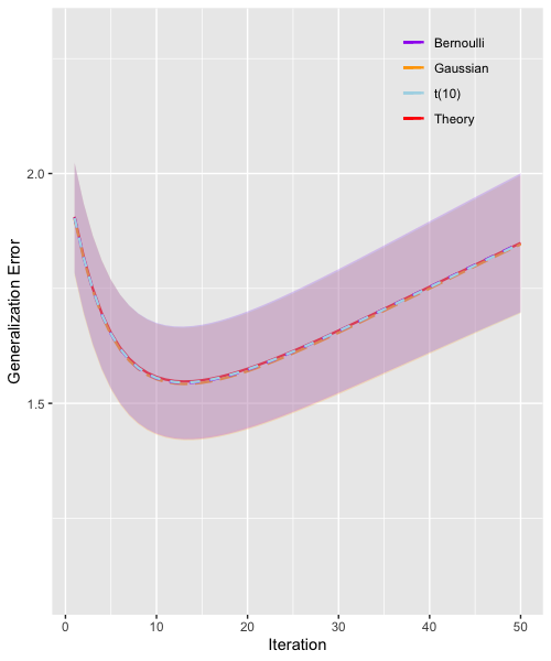
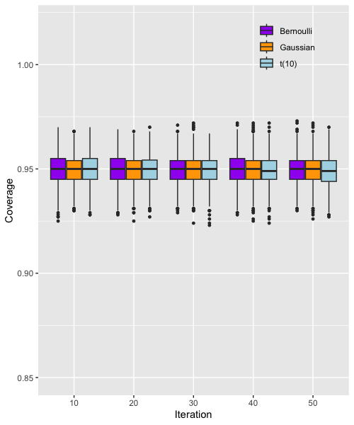
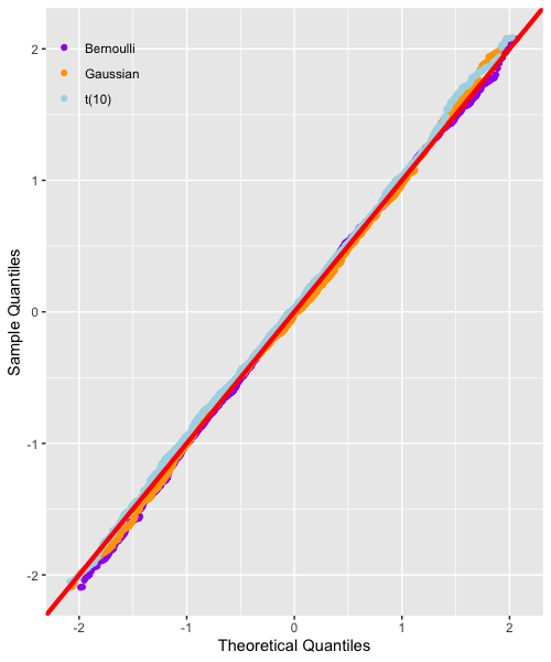
Figure 3. Linear regression model with Pseudo-Huber loss. Simulation parameters: $\eta=0.3$, $\mu_{\ast}\in\mathbb{R}^{n}$ are i.i.d. $\lvert\mathcal{N}(0,5)\rvert$, $\xi\in\mathbb{R}^{m}$ has i.i.d. entries drawn from a $t$ distribution with $2$ degrees of freedom.

Common numerical settings:

We set the sample size as $m=1200$ and the signal dimension as $n=1000$. The scaled random design matrix $\sqrt{n}A$ has i.i.d. entries following $\mathcal{N}(0,1)$ (orange), $t$ distribution with $10$ degrees of freedom (blue), Bernoulli$(1/2)$ (purple). The colors in parentheses correspond to those used in the figures. Proper normalization is applied to the latter two cases so that the variance is $1$. The gradient descent inference algorithm is run for $50$ iterations with Monte Carlo repetition $B=1000$.

Different simulation settings in two models:

1. (Linear regression model with pseudo-Huber loss). We examine the performance of the gradient descent inference algorithm in linear regression with following robust loss, known the pseudo-Huber function:

   $$\mathsf{L}_{\delta}(x,y)\equiv\delta^{2}\big{(}\{1+(x-y)^{2}/\delta^{2}\}^{1/2}-1\big{)},\quad\forall x,y\in\mathbb{R}.$$

   Clearly $\mathsf{L}_{\delta}$ satisfies the regularity conditions in Theorem 4.1 for any $\delta>0$. For definiteness, here we use $\delta=1$ as in the numerical experiment in [TB24, Section 4]. As the pseudo-Huber loss function is designed to accommodate heavy-tailed errors, here we choose the noises $\{\xi_{i}\}$ as i.i.d. $t$-distributed random variables with only 2 degrees of freedom.

2. (One-bit compressed sensing model with squared loss). We examine the performance of the gradient descent inference algorithm in the model (5.1) with the squared loss function, now under i.i.d. $\mathcal{N}(0,1)$ noises $\{\xi_{i}\}$. As mentioned in Section 5, the global minimizer under the squared loss has been proven to be consistent for a scaled version of $\mu_{\ast}$ in [HJLZ18] under Gaussian noises.

   In this setting, the signal strength $\sigma_{\mu_{\ast}}$ can be estimated by

   $$\widehat{\sigma}_{\mu_{\ast}}\equiv\bigg{(}\frac{\widehat{Q}(A,Y)}{1-\widehat{Q}(A,Y)}\bigg{)}^{1/2},\quad\widehat{Q}(A,Y)\equiv\frac{\pi}{2\phi}\bigg{(}\frac{\lVert A^{\top}Y\rVert^{2}}{m}-1\bigg{)}_{+}\wedge 1.$$ (C.1)

   To justify this estimator $\widehat{\sigma}_{\mu_{\ast}}$ for $\sigma_{\mu_{\ast}}$, consider the initialization $\mu^{(0)}=0$ and step size $\eta=1$. At iteration $1$, the debiased gradient descent iterate is given by $\mu^{(1)}_{\mathrm{db}}=\phi^{-1}A^{\top}Y$. Moreover, Proposition 5.4-(2) shows that $b^{(1)}_{\mathrm{db}}=2\operatorname{\mathbb{E}}^{(0)}\mathfrak{g}_{\sigma_{\mu_{\ast}}}(\xi_{\pi_{m}})\approx 2\operatorname{\mathbb{E}}\mathfrak{g}_{1}(\sigma_{\mu_{\ast}}\mathsf{Z})=2\big{(}2\pi(1+\sigma_{\mu_{\ast}}^{2})\big{)}^{-1/2}$ and $(\sigma^{(1)}_{\mathrm{db}})^{2}=\phi^{-1}$. Then applying Proposition 5.4-(1) leads to

   $$\phi^{-1}\frac{\lVert A^{\top}Y\rVert^{2}}{m}=\frac{\lVert\mu^{(1)}_{\mathrm{db}}\rVert^{2}}{n}\approx(b^{(1)}_{\mathrm{db}})^{2}\sigma_{\mu_{\ast}}^{2}+(\sigma^{(1)}_{\mathrm{db}})^{2}\approx\frac{2}{\pi}\cdot\frac{\sigma_{\mu_{\ast}}^{2}}{1+\sigma_{\mu_{\ast}}^{2}}+\phi^{-1}.$$

   The proposal (C.1) follows by inverting the above approximation.

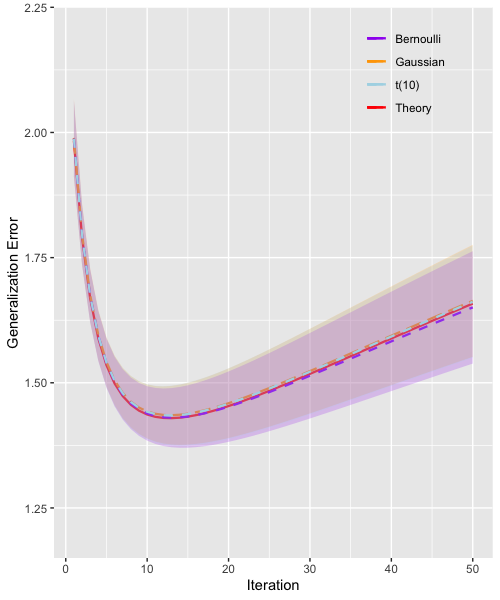
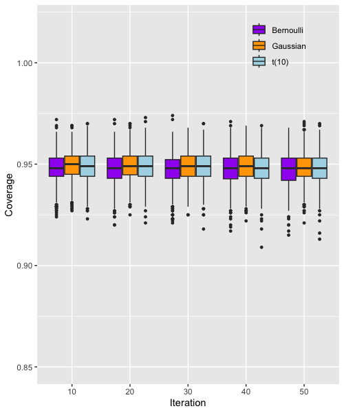
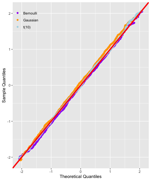
Figure 4. One-bit compressed sensing model with squared loss. Simulation parameters: $\eta=0.1$, $\mu_{\ast}\in\mathbb{R}^{n}$ are i.i.d. $\lvert\mathcal{N}(0,1)\rvert$, $\xi\in\mathbb{R}^{m}$ has i.i.d. $\mathcal{N}(0,1)$ entries.

Numerical findings:

We report the simulation results for (1) above in Figure 3, and for (2) above in Figure 4. Both of these figures further confirm the key findings discussed in Sections 4 and 5:

• The left panels in both figures highlight the early stopping phenomenon in gradient descent.

• The middle panels confirm that the CIs for both models achieve the nominal coverage level, demonstrating robust performance across varying settings.

• The right panels validate the distributional characterization of $\widehat{\mu}^{(t)}_{\mathrm{db}}$; specifically, we present $(\widehat{\mu}^{(t)}_{\mathrm{db};1}-\mu_{\ast;1})/\widehat{\sigma}^{(t)}_{\mathrm{db}}$ at the final iteration, showing strong agreement with theoretical predictions.

These findings are consistently observed across a wide range of simulation parameters. To avoid redundancy, we omit additional figures of a similar nature.

References

- [ABC20] Ada Altieri, Giulio Biroli, and Chiara Cammarota, Dynamical mean-field theory and aging dynamics, J. Phys. A 53 (2020), no. 37, 375006, 34.
- [ADT20] Alnur Ali, Edgar Dobriban, and Ryan Tibshirani, The implicit regularization of stochastic gradient flow for least squares, International conference on machine learning, PMLR, 2020, pp. 233–244.
- [AKT19] Alnur Ali, J Zico Kolter, and Ryan J Tibshirani, A continuous-time view of early stopping for least squares regression, The 22nd international conference on artificial intelligence and statistics, PMLR, 2019, pp. 1370–1378.
- [BAGJ21] Gérard Ben Arous, Reza Gheissari, and Aukosh Jagannath, Online stochastic gradient descent on non-convex losses from high-dimensional inference, J. Mach. Learn. Res. 22 (2021), Paper No. 106, 51.
- [BAGJ24] by same author, High-dimensional limit theorems for SGD: effective dynamics and critical scaling, Comm. Pure Appl. Math. 77 (2024), no. 3, 2030–2080.
- [Bel22] Pierre C. Bellec, Observable adjustments in single-index models for regularized M-estimators, arXiv preprint arXiv:2204.06990 (2022).
- [BGH23] Krishnakumar Balasubramanian, Promit Ghosal, and Ye He, High-dimensional scaling limits and fluctuations of online least-squares sgd with smooth covariance, arXiv preprint arXiv:2304.00707 (2023).
- [BHX23] Zhigang Bao, Qiyang Han, and Xiaocong Xu, A leave-one-out approach to approximate message passing, arXiv preprint arXiv:2312.05911 (2023).
- [BLM15] Mohsen Bayati, Marc Lelarge, and Andrea Montanari, Universality in polytope phase transitions and message passing algorithms, Ann. Appl. Probab. 25 (2015), no. 2, 753–822.
- [BM11] Mohsen Bayati and Andrea Montanari, The dynamics of message passing on dense graphs, with applications to compressed sensing, IEEE Trans. Inform. Theory 57 (2011), no. 2, 764–785.
- [BMN20] Raphaël Berthier, Andrea Montanari, and Phan-Minh Nguyen, State evolution for approximate message passing with non-separable functions, Inf. Inference 9 (2020), no. 1, 33–79.
- [BT24] Pierre C. Bellec and Kai Tan, Uncertainty quantification for iterative algorithms in linear models with application to early stopping, arXiv preprint arXiv:2404.17856 (2024).
- [BvdG11] Peter Bühlmann and Sara van de Geer, Statistics for high-dimensional data, Springer Series in Statistics, Springer, Heidelberg, 2011, Methods, theory and applications.
- [BZ23] Pierre C. Bellec and Cun-Hui Zhang, Debiasing convex regularized estimators and interval estimation in linear models, Ann. Statist. 51 (2023), no. 2, 391–436.
- [CCM21] Michael Celentano, Chen Cheng, and Andrea Montanari, The high-dimensional asymptotics of first order methods with random data, arXiv preprint arXiv:2112.07572 (2021).
- [CL21] Wei-Kuo Chen and Wai-Kit Lam, Universality of approximate message passing algorithms, Electron. J. Probab. 26 (2021), Paper No. 36, 44.
- [CLTZ20] Xi Chen, Jason D. Lee, Xin T. Tong, and Yichen Zhang, Statistical inference for model parameters in stochastic gradient descent, Ann. Statist. 48 (2020), no. 1, 251–273.
- [CMW23] Michael Celentano, Andrea Montanari, and Yuting Wei, The Lasso with general Gaussian designs with applications to hypothesis testing, Ann. Statist. 51 (2023), no. 5, 2194–2220.
- [CWPPS24] Elizabeth Collins-Woodfin, Courtney Paquette, Elliot Paquette, and Inbar Seroussi, Hitting the High-dimensional notes: an ODE for SGD learning dynamics on GLMs and multi-index models, Inf. Inference 13 (2024), no. 4, Paper No. iaae028.
- [DM16] David Donoho and Andrea Montanari, High dimensional robust M-estimation: asymptotic variance via approximate message passing, Probab. Theory Related Fields 166 (2016), no. 3-4, 935–969.
- [EK13] Noureddine El Karoui, Asymptotic behavior of unregularized and ridge-regularized high-dimensional robust regression estimators: rigorous results, arXiv preprint arXiv:1311.2445 (2013).
- [EK18] by same author, On the impact of predictor geometry on the performance on high-dimensional ridge-regularized generalized robust regression estimators, Probab. Theory Related Fields 170 (2018), no. 1-2, 95–175.
- [Fan22] Zhou Fan, Approximate message passing algorithms for rotationally invariant matrices, Ann. Statist. 50 (2022), no. 1, 197–224.
- [FXY18] Yixin Fang, Jinfeng Xu, and Lei Yang, Online bootstrap confidence intervals for the stochastic gradient descent estimator, J. Mach. Learn. Res. 19 (2018), Paper No. 78, 21.
- [GTM+24] Cédric Gerbelot, Emanuele Troiani, Francesca Mignacco, Florent Krzakala, and Lenka Zdeborová, Rigorous Dynamical Mean-Field Theory for Stochastic Gradient Descent Methods, SIAM J. Math. Data Sci. 6 (2024), no. 2, 400–427.
- [Han23] Qiyang Han, Noisy linear inverse problems under convex constraints: Exact risk asymptotics in high dimensions, Ann. Statist. 51 (2023), no. 4, 1611–1638.
- [Han24] by same author, Entrywise dynamics and universality of general first order methods, arXiv preprint arXiv:2406.19061 (2024).
- [HJLZ18] Jian Huang, Yuling Jiao, Xiliang Lu, and Liping Zhu, Robust decoding from 1-bit compressive sampling with ordinary and regularized least squares, SIAM J. Sci. Comput. 40 (2018), no. 4, A2062–A2086.
- [HMRT22] Trevor Hastie, Andrea Montanari, Saharon Rosset, and Ryan J. Tibshirani, Surprises in high-dimensional ridgeless least squares interpolation, Ann. Statist. 50 (2022), no. 2, 949–986.
- [HS23] Qiyang Han and Yandi Shen, Universality of regularized regression estimators in high dimensions, Ann. Statist. 51 (2023), no. 4, 1799–1823.
- [HX23] Qiyang Han and Xiaocong Xu, The distribution of ridgeless least squares interpolators, arXiv preprint arXiv:2307.02044 (2023).
- [JM13] Adel Javanmard and Andrea Montanari, State evolution for general approximate message passing algorithms, with applications to spatial coupling, Inf. Inference 2 (2013), no. 2, 115–144.
- [JM14] by same author, Confidence intervals and hypothesis testing for high-dimensional regression, J. Mach. Learn. Res. 15 (2014), 2869–2909.
- [Kol11] Vladimir Koltchinskii, Oracle inequalities in empirical risk minimization and sparse recovery problems, Lecture Notes in Mathematics, vol. 2033, Springer, Heidelberg, 2011, Lectures from the 38th Probability Summer School held in Saint-Flour, 2008, École d’Été de Probabilités de Saint-Flour. [Saint-Flour Probability Summer School].
- [MKUZ20] Francesca Mignacco, Florent Krzakala, Pierfrancesco Urbani, and Lenka Zdeborová, Dynamical mean-field theory for stochastic gradient descent in gaussian mixture classification, Advances in Neural Information Processing Systems 33 (2020), 9540–9550.
- [MM21] Léo Miolane and Andrea Montanari, The distribution of the Lasso: uniform control over sparse balls and adaptive parameter tuning, Ann. Statist. 49 (2021), no. 4, 2313–2335.
- [Mon18] Andrea Montanari, Mean field asymptotics in high-dimensional statistics: from exact results to efficient algorithms, Proceedings of the International Congress of Mathematicians—Rio de Janeiro 2018. Vol. IV. Invited lectures, World Sci. Publ., Hackensack, NJ, 2018, pp. 2973–2994.
- [MRSY23] Andrea Montanari, Feng Ruan, Youngtak Sohn, and Jun Yan, The generalization error of max-margin linear classifiers: Benign overfitting and high-dimensional asymptotics in the overparametrized regime, arXiv preprint arXiv:1911.01544v3 (2023).
- [MU22] Francesca Mignacco and Pierfrancesco Urbani, The effective noise of stochastic gradient descent, J. Stat. Mech. Theory Exp. (2022), no. 8, Paper No. 083405, 23.
- [PJ92] B. T. Polyak and A. B. Juditsky, Acceleration of stochastic approximation by averaging, SIAM J. Control Optim. 30 (1992), no. 4, 838–855.
- [PLPP21] Courtney Paquette, Kiwon Lee, Fabian Pedregosa, and Elliot Paquette, Sgd in the large: Average-case analysis, asymptotics, and stepsize criticality, Conference on Learning Theory, PMLR, 2021, pp. 3548–3626.
- [PP21] Courtney Paquette and Elliot Paquette, Dynamics of stochastic momentum methods on large-scale, quadratic models, Advances in Neural Information Processing Systems 34 (2021), 9229–9240.
- [Rup88] David Ruppert, Efficient estimations from a slowly convergent robbins-monro process, Tech. report, Cornell University Operations Research and Industrial Engineering, 1988.
- [SC19] Pragya Sur and Emmanuel J. Candès, A modern maximum-likelihood theory for high-dimensional logistic regression, Proc. Natl. Acad. Sci. 116 (2019), no. 29, 14516–14525.
- [SCC19] Pragya Sur, Yuxin Chen, and Emmanuel J. Candès, The likelihood ratio test in high-dimensional logistic regression is asymptotically a rescaled chi-square, Probab. Theory Related Fields 175 (2019), no. 1-2, 487–558.
- [Sto13] Mihailo Stojnic, A framework to characterize performance of lasso algorithms, arXiv preprint arXiv:1303.7291 (2013).
- [TAH18] Christos Thrampoulidis, Ehsan Abbasi, and Babak Hassibi, Precise error analysis of regularized -estimators in high dimensions, IEEE Trans. Inform. Theory 64 (2018), no. 8, 5592–5628.
- [TB24] Kai Tan and Pierre C Bellec, Estimating generalization performance along the trajectory of proximal sgd in robust regression, arXiv preprint arXiv:2410.02629 (2024).
- [TOH15] Christos Thrampoulidis, Samet Oymak, and Babak Hassibi, Regularized linear regression: A precise analysis of the estimation error, Conference on Learning Theory, PMLR, 2015, pp. 1683–1709.
- [vdG00] Sara van de Geer, Applications of Empirical Process Theory, Cambridge Series in Statistical and Probabilistic Mathematics, vol. 6, Cambridge University Press, Cambridge, 2000.
- [vdV98] Aad van der Vaart, Asymptotic Statistics, Cambridge Series in Statistical and Probabilistic Mathematics, vol. 3, Cambridge University Press, Cambridge, 1998.
- [vdVW96] Aad van der Vaart and Jon A. Wellner, Weak Convergence and Empirical Processes, Springer Series in Statistics, Springer-Verlag, New York, 1996.
- [Wai19] Martin J. Wainwright, High-dimensional statistics, Cambridge Series in Statistical and Probabilistic Mathematics, vol. 48, Cambridge University Press, Cambridge, 2019, A non-asymptotic viewpoint.
- [YYMD21] Steve Yadlowsky, Taedong Yun, Cory Y McLean, and Alexander D’Amour, SLOE: A faster method for statistical inference in high-dimensional logistic regression, Advances in Neural Information Processing Systems 34 (2021), 29517–29528.
- [ZCW23] Wanrong Zhu, Xi Chen, and Wei Biao Wu, Online covariance matrix estimation in stochastic gradient descent, J. Amer. Statist. Assoc. 118 (2023), no. 541, 393–404.