iKap: Kinematics-aware Planning with Imperative Learning

Abstract

Trajectory planning in robotics aims to generate collision-free pose sequences that can be reliably executed. Recently, vision-to-planning systems have garnered increasing attention for their efficiency and ability to interpret and adapt to surrounding environments. However, traditional modular systems suffer from increased latency and error propagation, while purely data-driven approaches often overlook the robot’s kinematic constraints. This oversight leads to discrepancies between planned trajectories and those that are executable. To address these challenges, we propose iKap, a novel vision-to-planning system that integrates the robot’s kinematic model directly into the learning pipeline. iKap employs a self-supervised learning approach and incorporates the state transition model within a differentiable bi-level optimization framework. This integration ensures the network learns collision-free waypoints while satisfying kinematic constraints, enabling gradient back-propagation for end-to-end training. Our experimental results demonstrate that iKap achieves higher success rates and reduced latency compared to the state-of-the-art methods. Besides the complete system, iKap offers a visual-to-planning network that seamlessly integrates kinematics into various controllers, providing a robust solution for robots navigating complex and dynamic environments.

I Introduction

Path planning is a fundamental task in robotics, involving the determination of a collision-free trajectory that connects the robot’s current position to the goal [1]. In dynamic and complex environments, robots must accurately perceive their surroundings and correlate environmental data with the planned path to ensure successful task execution [2]. Recently, with the development of perceptual systems, direct vision-to-planning systems have garnered increasing attention due to their potential efficiency and the ability to interpret and adapt to surrounding environments [3].

Traditional vision-to-planning systems often employ a modular design where the planning module operates with an independent perception module that processes sensor data to generate environmental representations [4]. While this modular approach offers clarity and flexibility, it introduces several challenges. Communicating intermediate results between modules leads to potential latency, increased communication overhead, and higher storage demands [5]. Moreover, errors in one module can propagate and amplify throughout the system, compromising overall performance [2].

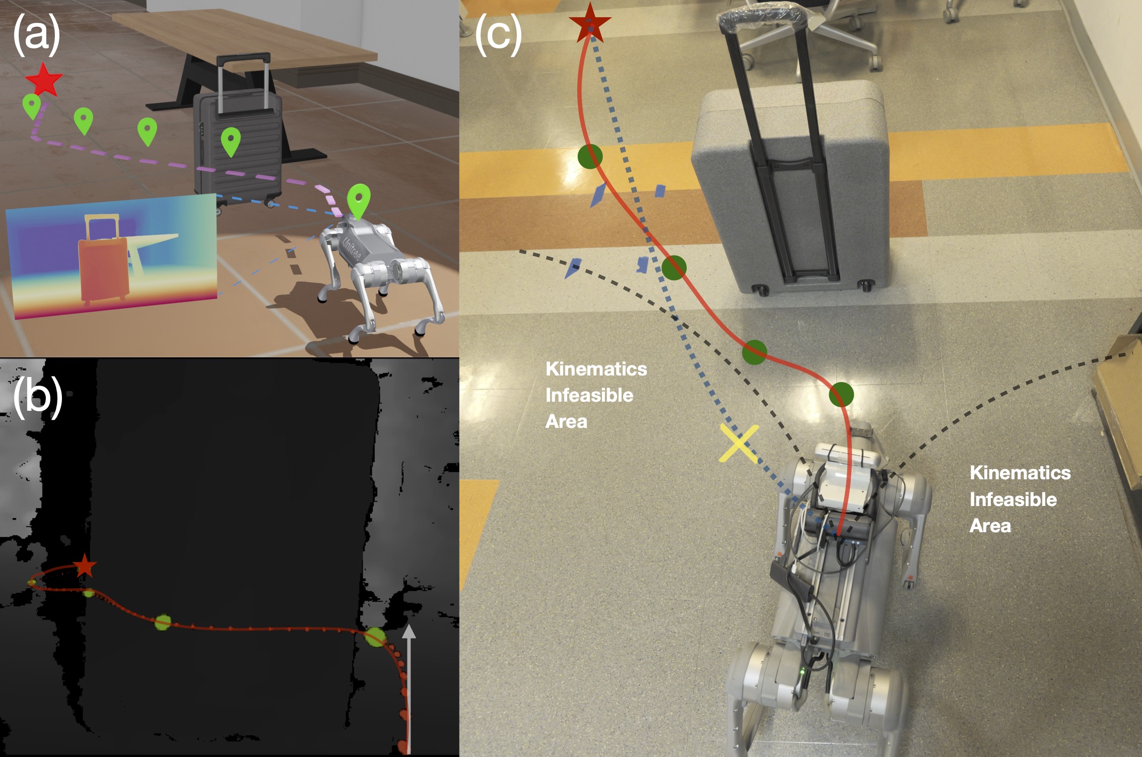
Figure 1: The kinematics-aware planner, iKap, incorporates kinematic state transition functions directly into the learning pipeline. This integration allows the network to learn feasible waypoint distributions and produce more executable trajectories. (a) The robot, constrained by a minimum turning radius, must reach the red star while avoiding obstacles. (b) A real-world depth image alongside the predicted trajectory. (c) A geometry-based planner may generate the blue trajectory, which does not satisfy the kinematic constraints, making it difficult to execute.

Data-driven end-to-end approaches, particularly those utilizing deep learning, have obtained significant advancement [3]. Such methods directly map sensor inputs to control outputs, eliminating the error propagation and latency inherent in modular systems [6, 7, 8, 3]. However, purely data-driven methods often act as black boxes, require vast amounts of data, have low sample efficiency, and exhibit a significant sim-to-real gap. In addition, these approaches lack interpretability, making it challenging to incorporate explicit physical constraints or prior knowledge [9]. Although recent works such as iPlanner [10] have explored combining data-driven methods with trajectory optimization, they neglect the robot’s kinematics. This absence of physical constraints can result in generated trajectories that are difficult for low-level controllers to execute, leading to issues such as deadlocks, collisions, or suboptimal performance [11]. As illustrated in Figure 1, for a robot with kinematic constraints like a minimum turning radius, the planned trajectory (blue curve) may not be executable by the robot.

To address the issue of previous end-to-end systems often generating infeasible paths, we argue that kinematic constraints should be incorporated into vision-to-planning networks while retaining the end-to-end learning architecture to avoid execution errors.

To this end, we propose an Imperative learning-based Kinematics-aware Planning (iKap) system that integrates the robot’s kinematic model directly into the learning pipeline. This system supervises the network to learn kinematically feasible trajectories through self-supervised bi-level optimization (BLO). The learning module of iKap is highly flexible and can be easily integrated with various controllers to plan executable trajectories. Our main contributions include:

• We integrate the robot’s kinematic model into the training pipeline through a differentiable model predictive control (MPC) using a self-supervised bi-level optimization framework via imperative training. This enables the network to learn the kinematically feasible trajectories.

• We develop a learning pipeline that enables gradient backpropagation from the lower-level trajectory optimization to the upper-level network parameters, facilitating a kinematics-aware vision-to-planning model.

• We present both simulation and real-world experiments to evaluate the proposed system in various environments. Results show that iKap achieves a higher success rate and lower tracking error than the baseline approach.

II Related Work

II-A Data-driven Planner

Our research builds upon iPlanner [10], an end-to-end local planner that formulates trajectory planning as a bi-level optimization problem. iPlanner guides neural networks to plan collision-free paths using an imperative loss based on the Euclidean Signed Distance Field (ESDF). However, it assumes that robots can perfectly execute trajectories optimized purely from geometric constraints, neglecting kinematic feasibility and thus limiting real-world performance, especially for agile robots. Additionally, iPlanner simplifies the bi-level optimization to a single-level problem via a closed-form solution for the lower-level problem, enhancing computational efficiency but reducing generalizability to other constraints. ViPlanner [12] extends iPlanner by incorporating semantic information to construct cost maps for semantic-based local planning, yet it does not address the limitations regarding kinematic feasibility and generalizability.

Notable works like NoMaD [3] utilize transformer-based architectures for action diffusion and motion prediction, integrating past observations with optional goal states to enhance decision-making. Similarly, ViNT [13] employs a transformer-based architecture to directly convert visual inputs into navigation decisions, enabling seamless adaptation across various environments and tasks. However, these methods lack physical representation during their training processes, potentially limiting their ability to account for dynamic and kinematic constraints. Efforts to integrate physical models into data-driven planning include DIPP [14], which combines a transformer with a differentiable trajectory model to plan based on road conditions and historical agent data. This approach requires supervised learning with labeled data, and the transformer architecture introduces latency, affecting real-time performance. PhysORD [15] applies Lagrangian mechanics as a constraint for off-road driving motion prediction but does not incorporate visual data into the pipeline. Gao et al. [16] demonstrated that embedding neural networks with safe corridors and trajectory optimization can efficiently generate collision-free and dynamically feasible trajectories, particularly for drones; however, it relies on supervised learning with results limited to simulations.

Differentiable simulation has recently gained increasing attention for its ability to accelerate model learning by leveraging autodiff tools to compute the gradient propagation of system dynamics. Previous studies have demonstrated that integrating differentiable simulation into reinforcement learning systems significantly improves sample efficiency, enabling applications in vision-based control tasks [17]. Furthermore, recent work has integrated a simple point-mass model with a deep learning pipeline and achieved visual-based navigation tasks by introducing temporal gradient decay to mitigate gradient explosion [18].

II-B Differentiable Optimization and Imperative Learning

Traditional robotics algorithms often rely on optimization techniques, which can establish implicit relationships between input and output data. Integrating optimization-based algorithms into end-to-end systems can narrow the search space for neural networks, reduce the number of parameters, and improve computational efficiency [16].

In this context, the differentiable optimization solver is critical, ensuring correct gradient propagation during the learning process. Amos et al. proposed implicit differentiation to manage gradient backpropagation for argmin problems, integrating this process as a layer in neural networks. In their follow-up work, they introduced differentiable MPC, which plays a significant role in bridging optimization with deep learning frameworks [19, 20].

In addition, incorporating differentiable optimization into end-to-end training frameworks also preserves the interpretability of classical methods. This integration offers a promising avenue for developing more sophisticated and interpretable robotic systems. Building on these concepts, imperative learning has been proposed. It incorporates optimization-based algorithms as constraints, adapting to the robot’s state and facilitating self-supervised learning [21]. Ultimately, the network training problem can be formulated as a bi-level optimization. However, a critical challenge is the gradient backpropagation from the upper-level to the lower-level optimization, which was bypassed by many previous works either using closed-form solutions [10], gradient assumptions at convergence [22, 23], or discrete approximations [24, 25]. Our problem relies heavily on accurate gradient due to the necessity of physical constraint in the BLO and strong coupling between the two level optimization. We address this issue by employing a differentiable MPC [26, 27], demonstrating that imperative learning can successfully operate in scenarios with constraint optimization. This confirms the versatility and robustness of this architecture in complex robotic applications.

III Method

III-A Problem Formulation and System Overview

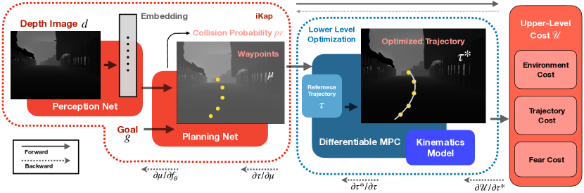
Figure 2: The training pipeline for the planner is based on bi-level optimization. In this framework, the networks, the optimized object, generate waypoints based on the given depth perception and goals. Then, the low-level trajectory optimization module tracks a kinematics-feasible trajectory. The embedded kinematics and gradients from the lower-level module are then utilized to supervise and train the networks.

At time stamp $t$, given observed depth image $\mathcal{D}_{t}$ and a target location $\mathbf{p}_{t}^{g}$ in the workspace $\mathcal{Q}\subset\mathbb{R}^{2}$, the planning problem is to find a trajectory $\mathbf{p}_{1:T+1}$ guiding the robot from the current position to the target while avoiding obstacles.

As illustrated in Fig. 2, our iKap consists of three key parts. First, a ResNet[28] front-end takes the depth observation $\mathcal{D}_{t}$ and encodes it into observation embedding. This embedding, combined with the target $\mathbf{p}_{t}^{g}$, is fed into the second planning network to predict a sparse key point trajectory $\boldsymbol{\mu}_{1:k}$ and collision probability $pr_{t}$. Third, a differentiable MPC tracks a reference $\boldsymbol{\tau}:=\mathbf{x}_{1:T+1}\in\mathcal{X}^{T+1}$ interpolated from $\boldsymbol{\mu}_{1:k}$ with time horizon $T$ and outputs the optimized trajectory $\boldsymbol{\tau}^{*}_{1:T+1}$ and action $\mathbf{u}^{*}_{1:T}$ while ensuring the kinematic feasibility $\mathbf{x}_{t+1}=\mathbf{F}(\mathbf{x}_{t},\mathbf{u}_{t})$. Here, $\mathbf{F}$ is the robot kinematics, $\mathbf{x}_{t}$ and $\mathbf{u}_{t}$ are the robot’s states and control input in configuration space $\mathcal{X}$ and action space $\mathcal{A}$, respectively. Finally, a well-designed traversability costs $\mathcal{U}$ is evaluated and backpropagated through both the differentiable MPC and the perception network to update the network parameters $\theta$. This process results in a bi-level optimization (BLO) problem (1), where perception and planning network is jointly optimized with the differentiable MPC.

$$\min_{\theta}\quad \mathcal{U}(\boldsymbol{\mu}_{1:k},\boldsymbol{\tau}^{*}),$$ (1a)

s.t. $$\boldsymbol{\tau}^{*}=\operatorname*{arg\,min}_{\mathbf{u}_{1:T}}\mathcal{L}(\boldsymbol{\mu}_{1:k},\mathbf{u}_{1:T}),$$ (1b)

$$\textrm{s.t.}\quad\mathbf{x}_{t+1}=\mathbf{F}(\mathbf{x}_{t},\mathbf{u}_{t}),$$ (1c)

$$\quad\quad\quad\ \mathbf{x}_{0}=\mathbf{0},$$ (1d)

where $\mathcal{L}$ denotes the cost of MPC. Intuitively, the upper-level cost $\mathcal{U}$ is iteratively updated based on the lower-level MPC, which can be optimized without providing labels, enabling a self-supervised learning process. Moreover, during the optimization, $\mathcal{U}$ consistently incorporates the robot’s kinematic models through the lower-level MPC, ensuring a kinematics-aware planning network. We next present the details of the planning module and MPC in Section III-B and Section III-C, respectively. The upper-level cost together with the method solving BLO will be illustrated in Section III-D.

III-B Perception and Planning Networks

The network consists of two components: the perception network, which processes depth images, and the planning network, which generates a trajectory based on the goal position and the output of the perception network.

III-B1 Perception Network

We use a similar network structure as in [10] for perception. At each timestep $t$, the robot’s sensor captures depth images $\mathcal{D}_{t}$. These images are processed by the perception network, which employs an enhanced ResNet architecture [28] to extract high-dimensional spatial features. After the encoder stage, the depth images are transformed into a higher-dimensional representation $\mathcal{O}_{t}\in\mathbb{R}^{C\times M}$, where $C=512$ denotes the number of channels and $M=240$ represents the dimension of the feature space.

III-B2 Planning Network

The planning module employs the embedding from perception network $\mathcal{O}_{t}\in\mathbb{R}^{C\times M}$ together with the goal position $\mathbf{p}_{t}^{g}\in\mathbb{R}^{2}$ to generate waypoints. To align the goal position with the embedding’s dimensionality, $\mathbf{p}_{t}^{g}$ is mapped into a higher-dimensional space $\mathcal{P}_{t}\in\mathbb{R}^{C^{*}\times M}$ via a simple multilayer perceptron (MLP). The embedding $\mathcal{O}_{t}$ and the transformed goal position $\mathcal{P}_{t}$ are then concatenated to form the final input $\hat{\mathcal{O}}\in\mathbb{R}^{C^{\prime}\times M}$, where $C^{\prime}=C+C^{*}$. The planning network, consisting of CNN and MLP with activation functions, predicts waypoints $\mathcal{K}_{t}\in\mathbb{R}^{n\times 2}$, where $n$ represents the number of key points.

III-C Differentiable Model-Predictive Control

We leverage a differentiable MPC module to incorporate the robot kinematic model into the training pipeline. The MPC can generate trajectories that comply with kinematic constraints, which can be formulated as:

$$\boldsymbol{\tau}^{*}= \ \operatorname*{arg\,min}_{\mathbf{x}_{1:T},\mathbf{u}_{1:T}}\ \sum_{t=0}^{T-1}(\tilde{\mathbf{x}}^{\top}_{t}\mathbf{Q}_{t}\tilde{\mathbf{x}}_{t}+\mathbf{u}_{t}^{\top}\mathbf{R}_{t}\mathbf{u}_{t})+\tilde{\mathbf{x}}^{\top}_{T}\mathbf{Q}_{T}\tilde{\mathbf{x}}_{T}$$ (2)

$$\quad\textrm{s.t.}\quad\mathbf{x}_{t+1}=\mathbf{F}(\mathbf{x}_{t},\mathbf{u}_{t}),$$ (3)

$$\quad\quad\quad~\mathbf{x}_{0}=\mathbf{0},$$ (4)

where $\tilde{\mathbf{x}}_{t}=\mathbf{x}_{t}-\mathbf{x}_{t}^{\text{ref}},t=0,\cdots,T$ is the error state between the current state $\mathbf{x}_{t}$ and reference trajectory $\mathbf{x}^{\text{ref}}$; $\tilde{\mathbf{x}}^{\top}_{t}\mathbf{Q}_{t}\tilde{\mathbf{x}}_{t}+\mathbf{u}_{t}^{\top}\mathbf{R}_{t}\mathbf{u}_{t}$ is the stage cost balancing the state and control effort; $\tilde{\mathbf{x}}^{\top}_{T}\mathbf{Q}_{T}\tilde{\mathbf{x}}_{T}$ is the terminal cost; $\mathbf{Q}_{t}$, $\mathbf{R}_{t}$,$\mathbf{Q}_{T}$ are the weight matrices. Specifically, the reference trajectory is obtained by interpolating the waypoints predicted by the planning network. The classic Dubins car (5) can be used to describe kinematic model of a legged robot.

$$\dot{x}_{t}=v\cos\theta_{t},\quad\dot{y}_{t}=v\sin\theta_{t},\quad\dot{\psi}_{t}=u_{t},$$ (5)

where $\mathbf{x}_{t}=[x_{t},y_{t},\psi_{t}]^{\top}$ is the robot states representing the position and heading and $\mathbf{u}_{t}=[v,u_{t}]^{\top}$ is the control input including the robot speed and turn rate. We then discretize (5) and use it as the kinematic constraint for (2). To avoid motion singularity and gradient instability for complex trajectories, we use $\mathbf{SE}(2)$ Lie group operation for robot kinematics.

Since $\boldsymbol{\tau}^{*}$ is a function of the reference path $\boldsymbol{\tau}$, which is a function of the predicted key point path $\boldsymbol{\mu}_{1:k}$ or $f_{\theta}$, and will be passed to the upper level optimization for the final end-to-end training, the critical part is to calculate the gradient $\frac{\partial\boldsymbol{\tau}^{*}}{\partial\boldsymbol{\tau}}$. The traditional unrolling approach maintain the computational graph throughout the entire iteration process [21], which poses significant computation burden when dealing with complex problem. It may also run into divergent or vanishing. Instead, we employ the implicit function differentiation theorem and leveraging the KKT condition of (2) at the optimal point to compute the gradients of the parameters [20]. Thus, there is no need for explicit unrolling of the entire iteration process. In practice, we use the differentiable MPC module in our robot learning library PyPose [29, 26], which solves the MPC by the iterative Linear Quadratic Regulator (iLQR) algorithm [27]. PyPose MPC adopts a more general and problem-agnostic automatic differentiation (AD)-based solution that introduces just one additional optimization iteration at the optimal point in the forward pass. This allows automatic gradient calculation during the backward pass without the need to differentiate through the entire unrolled chain or compute problem-specific analytical derivatives.

III-D Upper-level Cost Design and Optimization

To achieve self-supervised learning with BLO, an important component is the upper-level cost design and accurate gradient back-propagation. We formulate the upper-level cost function as a weighted summation of fear cost $\mathcal{C}^{\mathcal{F}}$, environment cost $\mathcal{C}^{\mathcal{E}}$, and trajectory cost $\mathcal{C}^{\mathcal{T}}$:

$$\mathcal{U}(\boldsymbol{\tau},\boldsymbol{\mu}_{1:k})=\alpha\cdot\mathcal{C}^{\mathcal{F}}(\boldsymbol{\tau})+\beta\cdot\mathcal{C}^{\mathcal{E}}(\boldsymbol{\tau},\boldsymbol{\mu}_{1:k})+\gamma\cdot\mathcal{C}^{\mathcal{T}}(\boldsymbol{\tau}).$$ (6)

As described in Section III-B, the planner network predicts a collision probability $pr_{t}$ along with the key point path. The fear cost $\mathcal{C}^{\mathcal{F}}$ in (7) computes the binary cross entropy (BCE) as the task-level cost to avoid collisions.

$$\mathcal{C}^{\mathcal{F}}=\begin{cases}\operatorname{BCELoss}(pr_{t},0.0)&\mathbf{p}\cap\mathcal{Q}_{obs}\neq\emptyset,\\ \operatorname{BCELoss}(pr_{t},1.0)&\text{ otherwise}.\end{cases}$$ (7)

The environmental cost $\mathcal{C}^{\mathcal{E}}$ in (8) represents the interaction cost between the environment and the trajectory during planning. The shortest distance between the robot and the environment, i.e., ESDF map, is used to ensure safety.

$$\mathcal{C}^{\mathcal{E}}=\frac{1}{k}\sum_{i=1}^{k}\rm{ESDF}_{\mathcal{E}}(\boldsymbol{\mu}_{i})+\frac{1}{T}\sum_{i=1}^{T}\rm{ESDF}_{\mathcal{E}}(\mathbf{p}_{i}).$$ (8)

The trajectory cost $\mathcal{C}^{\mathcal{T}}$ in (9), consisting of three terms, is to evaluate the trajectory shape and trackability.

$$\mathcal{C}^{\mathcal{T}}= \gamma_{1}\cdot\log(\|\boldsymbol{\mu}_{k}-\mathbf{p}_{t}^{g}\|_{2}+1.0)$$ (9)

$$+ \gamma_{2}\cdot\frac{1}{T-1}\sum_{i=2}^{T}\|\frac{i\cdot\boldsymbol{\mu}_{k}}{T}-\mathbf{p}_{i}\|_{2}$$

$$+ \gamma_{3}\cdot\frac{1}{T}\sum_{i=2}^{T+1}\|\tilde{\mathbf{x}}_{i}\|_{2}.$$

The first term encourages the planner to generate a trajectory close to the goal. The second term measures the deviation from a straight, uniformly distributed path, ensuring that the trajectory is evenly spaced. This design also helps smooth out disorganized paths, preventing the learning process from becoming trapped in local minima. The final term focuses on the relationship between the reference and kinematics-feasible trajectory. Minimizing it allows the network to learn the distribution of kinematically feasible trajectories.

To solve the BLO in (1), the gradient of the upper-level cost must be propagated back through the lower-level system by applying the chain rule, and the network parameter is updated using gradient decent:

$$\nabla_{\theta}\mathcal{U}=(\frac{\partial\mathcal{U}}{\partial\boldsymbol{\mu}}+\frac{\partial\mathcal{U}}{\partial\boldsymbol{\tau}^{*}}\boldsymbol{\frac{\partial\tau^{*}}{\partial\boldsymbol{\tau}}}\boldsymbol{\frac{\partial\tau}{\partial\boldsymbol{\mu}}})\frac{\partial\boldsymbol{\mu}}{\partial\theta}$$ (10)

$$\theta_{t+1}=\theta_{t}-\alpha\cdot\nabla_{\theta}\mathcal{U}.$$ (11)

where $\alpha$ is the learning rate. Notice that most of the gradient terms in (11) can be computed automatically in PyTorch. However, the relationship between the reference trajectory $\boldsymbol{\tau}$ and the optimized trajectory $\boldsymbol{\tau}^{*}$ is determined through an $\rm{argmin}$ optimization, which is difficult to compute. Using the differentiable MPC in PyPose [29], we can resolve this through implicit differentiation.

IV Experiments

IV-A Implementation, Platforms, and Baselines

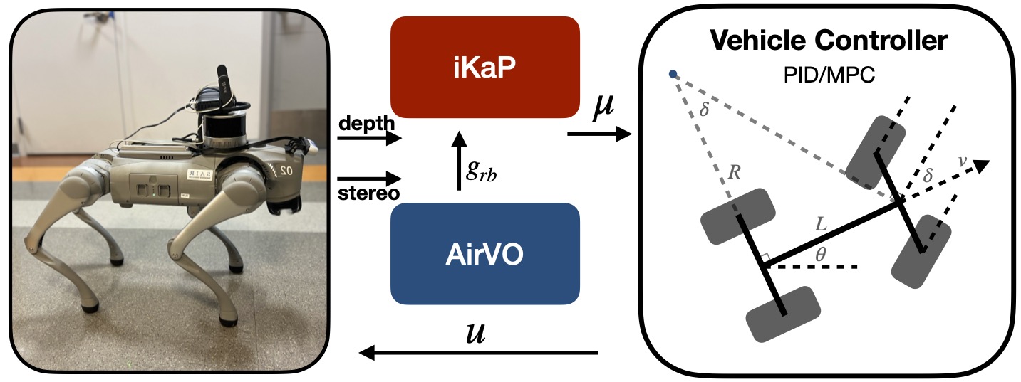
Figure 3: The real-world experiment pipeline. The experiments are conducted on the Unitree Go2 robot dog. We use AirVO to estimate the robot’s odometry, command the goal waypoint to the robot, and inputs this information into iKap along with depth images captured by the RealSense D435i camera.

We next evaluate the performance of iKap in both simulated and real-world settings. Specifically, we employ the simulated environments for autonomous exploration provided in [30], running on a desktop equipped with an Intel i7-12700k CPU and an Nvidia RTX 3090 GPU. For real-world experiments, we deploy the Unitree GO2 legged robot as shown in Fig. 3, outfitted with an Intel RealSense D435i camera that offers depth and stereo perception at 30 Hz. To assess generalization capability, we collect training data only from simulations, where the robot is joystick-controlled in four different environments: forests, garage, indoor, and Matterport3D [31]. We implement the stereo odometry solution AirVO [32] to track the robot’s position and generate an ESDF map. The training process, executed on an A6000 GPU, takes approximately six hours.

As a baseline model, we adopt the pre-trained iPlanner [10]. To facilitate clarity, we summarize the following settings both for baselines and our proposed method:

1. iKap: This is Our proposed planning network as is presented in Section III. It is jointly trained with Dubins car model and allows plug-and-play replacement by different low-level controllers designed for other kinematics.

2. iKap+PID: This setting is at test time. We use a PID controller to track iKap planned reference trajecotry.

3. iKap+MPC: This setting is at test time. We use an MPC controller to track iKap planned reference trajecotry.

4. iPlanner This is the baseline setting and it differs from Ours in that it is trained without kinematics embeddings.

IV-B System Performance

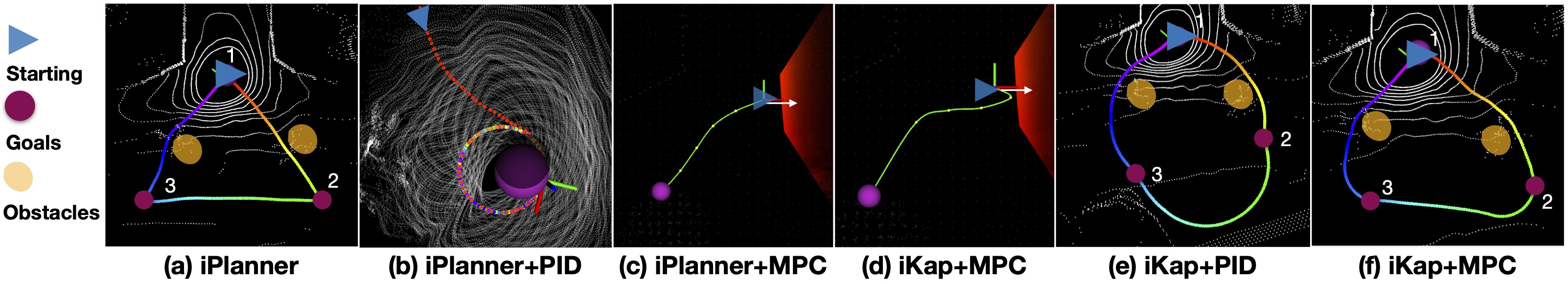
Figure 4: Qualitative performance. (a) iPlanner without controller: The planner generates sharp-angled trajectories that are difficult to execute. (b) iPlanner with PID controller: Without considering kinematics, iPlanner accumulates significant tracking errors, making control challenging. Near the goal, these errors cause iPlanner to get stuck in a looping behavior. (c, d) U-turn tests: iPlanner (c) generates backward trajectories, which are difficult for the MPC controller to execute. In contrast, iKap+MPC in (d) plans feasible trajectories that the controller can follow. (e, f) Trajectory Tracking: Using PID (e) and MPC (f) to track the waypoints generated by iKap. The robot can navigate robustly.

TABLE I: Average Tracking Error (unit: m) ($\downarrow$)

Controller	Method	Forests	Garage	Indoor	Matterport
PID	iPlanner	0.2084	0.2542	0.3157	0.3594
	iKap	0.1946	0.2394	0.2302	0.3387
MPC	iPlanner	0.1202	0.2137	0.1218	0.3025
	iKap	0.0832	0.1446	0.1042	0.2568

To demonstrate the flexibility and generalization capability of the proposed method, we conduct zero-shot transfer tests by applying a pre-trained model, initially embedded with a Dubins car model, to an unseen low-level bicycle model both in simulation and real world. Additionally, we employ two different controllers, PID and MPC to follow the reference trajectories generated by the iKap module.

IV-B1 Qualitative Result

An important factor in evaluating the effectiveness of the reference trajectory generated by the planner, is that it can be successfully tracked by different low-level controllers and robots with varying kinematics. iPlanner’s assumptions are highly limited, as it only considers geometric constraints of the trajectory. Fig. 4 (a) illustrates the trajectory produced by iPlanner when the target point is at the vertex of a star-shaped pattern. To follow such a trajectory, the robot must turn in place before executing the next segment, which is difficult for robots with other configurations. Fig. 4 (b) shows the compounding error issue when a robot modeled with bicycle kinematics uses a PID controller to track the iPlanner trajectory. If the tracking error falls within a critical range smaller than the robot’s minimum turning radius, the robot may continuously circle around the target point, leading to tracking failure. In U-turn tests where the goal position is behind the robot, iPlanner generates a trajectory like the one in Fig. 4 (c), whereas iKap generates a trajectory with a turning angle, as shown in Fig. 4 (d), providing the MPC controller with a more kinematically feasible starting point, thus reducing the gap between the planner and controller. Fig. 4 (e) illustrates the actual trajectory executed using a PID controller when static obstacles are present along the path. Similarly, Fig. 4 (f) depicts the trajectory executed by iKap+MPC, demonstrating stable planning capabilities and effective obstacle avoidance.

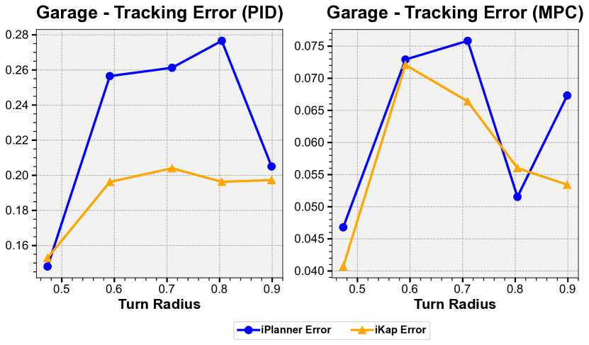
Figure 5: The trajectory tracking error against the minimum turning radius by PID and MPC controller in Garage simulation environment

IV-B2 Kinematic Feasibility

To evaluate the kinematic feasibility of different planners, we next show the tracking errors of generated paths executed by the controllers. To this end, we collect 200 depth images and goal pairs from the four simulation environments. We then calculate the mean squared error between the planned trajectories and trajectory executed by a controller, assuming a minimum turning radius of 1.48 meters. As shown in Table I, iKap reduces the tracking error by 11.85% with the PID controller and by 22.34% with the MPC controller, compared to iPlanner, across the four environments. This demonstrates significant advantages of iKap compared to iPlanner when given kinematic constraints.

To further show the performance of kinematic feasibility, we illustrate the tracking error in terms of turning radius by adjusting the maximum steering angle of the front wheels. As shown in Fig. 5, iKap can easily incorporate different minimum turning radius constraints and shows fewer tracking errors than iPlanner, demonstrating the flexibility of iKap in terms of kinematics-aware planning. This experiment demonstrates that iKap is robust to parameter variations, consistently generating kinematics-aware waypoints that are easier to track under different constraint conditions.

IV-B3 Navigation Test

We next evaluate the planners’ performance in a navigation task. To this end, we calculate the failure rate of a planner, where a failed attempt is defined as any instance where a collision with the environment occurred, the robot became deadlocked during planning, or the trajectory could not be executed by the controller. Specifically, we collected 100 pairs of start poses and goal positions and used both iPlanner and iKap to generate local trajectories and navigate the robot to its destination. As shown in Table II, iKap demonstrates superior performance in three environments. It can be seen that failure rate of iKap is slightly higher than in the “Garage” environment, this is because the robot often faces obstructed vision due to the presence of numerous walls and blind spots, while iKap is sensitive to that kinematic infeasible region.

TABLE II: Success Rate (%) (with MPC Controller) ($\uparrow$)

	Forests	Garage	Indoor	Campus
iPlanner	70.59	73.91	87.10	79.31
iKap	82.35	69.57	93.54	86.20

IV-B4 Real-time Demo on Real Robot

To evaluate the real-time online planning capabilities of iKap in real-world environments, we conduct tests using the quadruped robot Unitree GO2 equipped with an Intel RealSense D435i camera for depth perception. The robot operates with bicycle kinematics model, featuring a minimum turning radius of 0.73 meter. The depth measurements are inherently noisy and can suffer from distribution shifts compared to simulation data. Despite these challenges, our planning network, although trained exclusively in simulation without fine-tuning on real-world data, demonstrates strong generalization to real robot deployment. As shown in Fig. 6, the robot can conduct challenging navigation tasks where the robot starts indoors, passes through a narrow corridor, circles around a public area, and returns to the room along the same path. Additionally, we command the robot to go from off-road to on-road with a large stone blocking it. During this process, the human operator is responsible for sending goal points, while local navigation is autonomously managed by the planner.

To further increase the difficulty of the experiment, we place static obstacles, such as tables and chairs, in the open area of the public space, and have volunteers randomly walk along the robot’s path. The experimental results show that when the quadruped encounters obstacles that clearly block its path, it plans a smooth, kinematically feasible trajectory for easier tracking, rather than turning in place to adjust its heading before moving in a straight line. This navigation behavior improves the overall planning speed and enhances the robustness of the trajectory tracking performance by different types of low-level controllers such as PID and MPC.

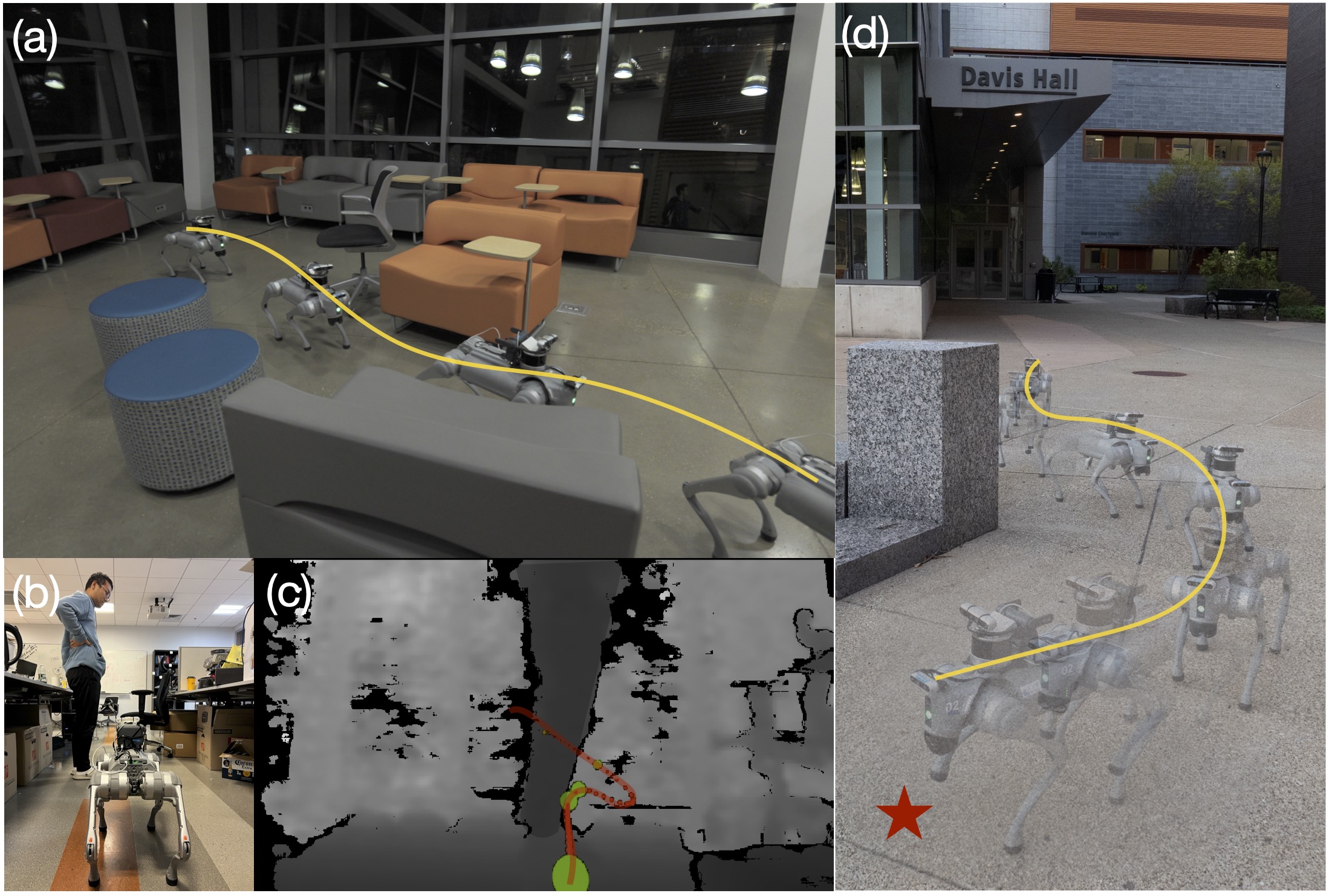
Figure 6: Snapshots of testing iKaP in real-world scenarios, including narrow rooms, open areas with obstacles, like humans, chairs and sofas, and outdoor environments. (a) The robot is commanded to a goal 5 meters ahead in an irregular, partially blocked open area; (b) The robot navigates a narrow path between a chair and a human; (c) shows its depth measurements and planned path; (d) The robot is commanded to move from off-road to on-road (red star) with a stone blocking the way.

V Conclusion and Limitation

We present iKap, a novel planning system that integrates kinematics into an end-to-end learning pipeline for path planning and control. By combining depth perception with a differentiable MPC module, iKap predicts dynamically feasible waypoints while ensuring that the planned trajectories comply with the robot’s kinematic constraints. Experimental results demonstrate that iKap enhances success rates in complex simulated environments and operates effectively under real-world conditions even with noisy depth perception, making it a promising solution for practical robot navigation. However, a limitation of this work is that we have only tested our model in human-made structured environments. In the future, we plan to extend iKap by developing a time-varying cost map for dynamic obstacles and testing the real-world performance under various environments.

References

- [1] S. Thrun, W. Burgard, and D. Fox, Probabilistic Robotics. MIT Press, 2005.
- [2] C. Cadena, L. Carlone, H. Carrillo, Y. Latif, D. Scaramuzza, J. Neira, I. Reid, and J. J. Leonard, “Past, present, and future of simultaneous localization and mapping: Toward the robust-perception age,” IEEE Transactions on Robotics, vol. 32, no. 6, pp. 1309–1332, 2016.
- [3] A. Sridhar, D. Shah, C. Glossop, and S. Levine, “NoMaD: Goal Masked Diffusion Policies for Navigation and Exploration,” Oct. 2023. [Online]. Available: https://arxiv.org/abs/2310.07896v1
- [4] F. Yang, C. Cao, H. Zhu, J. Oh, and J. Zhang, “Far planner: Fast, attemptable route planner using dynamic visibility update,” 2022. [Online]. Available: https://arxiv.org/abs/2110.09460
- [5] A. Loquercio, E. Kaufmann, R. Ranftl, M. Müller, V. Koltun, and D. Scaramuzza, “Learning high-speed flight in the wild,” Science Robotics, vol. 6, no. 59, p. eabg5810, 2021. [Online]. Available: https://www.science.org/doi/abs/10.1126/scirobotics.abg5810
- [6] M. Bojarski et al., “End to end learning for self-driving cars,” NVIDIA, Tech. Rep., 2016.
- [7] A. Amini, G. Rosman, S. Karaman, and D. Rus, “Variational End-to-End Navigation and Localization,” in 2019 International Conference on Robotics and Automation (ICRA), May 2019, pp. 8958–8964, arXiv:1811.10119 [cs, stat]. [Online]. Available: http://arxiv.org/abs/1811.10119
- [8] Z. Liu, A. Amini, S. Zhu, S. Karaman, S. Han, and D. Rus, “Efficient and Robust LiDAR-Based End-to-End Navigation,” May 2021, arXiv:2105.09932 [cs]. [Online]. Available: http://arxiv.org/abs/2105.09932
- [9] A. Sauer, N. Savva, and A. Geiger, “Conditional affordance learning for driving in urban environments,” in Conference on Robot Learning, 2018, pp. 237–252.
- [10] F. Yang, C. Wang, C. Cadena, and M. Hutter, “iPlanner: Imperative Path Planning,” in Robotics: Science and Systems XIX. Robotics: Science and Systems Foundation, Jul. 2023. [Online]. Available: http://www.roboticsproceedings.org/rss19/p064.pdf
- [11] Y. Kuwata et al., “Real-time motion planning with applications to autonomous urban driving,” IEEE Transactions on Control Systems Technology, vol. 17, no. 5, pp. 1105–1118, 2009.
- [12] P. Roth, J. Nubert, F. Yang, M. Mittal, and M. Hutter, “ViPlanner: Visual Semantic Imperative Learning for Local Navigation,” Oct. 2023, arXiv:2310.00982 [cs]. [Online]. Available: http://arxiv.org/abs/2310.00982
- [13] D. Shah, A. Sridhar, N. Dashora, K. Stachowicz, K. Black, N. Hirose, and S. Levine, “Vint: A foundation model for visual navigation,” 2023. [Online]. Available: https://arxiv.org/abs/2306.14846
- [14] Z. Huang, H. Liu, J. Wu, and C. Lv, “Differentiable integrated motion prediction and planning with learnable cost function for autonomous driving,” IEEE Transactions on Neural Networks and Learning Systems, pp. 1–15, 2023.
- [15] Z. Zhao, B. Li, Y. Du, T. Fu, and C. Wang, “PhysORD: A Neuro-Symbolic Approach for Physics-infused Motion Prediction in Off-road Driving,” Apr. 2024, arXiv:2404.01596 [cs]. [Online]. Available: http://arxiv.org/abs/2404.01596
- [16] Z. Han, L. Xu, and F. Gao, “Learning to plan maneuverable and agile flight trajectory with optimization embedded networks,” 2024. [Online]. Available: https://arxiv.org/abs/2405.07736
- [17] J. Heeg, Y. Song, and D. Scaramuzza, “Learning quadrotor control from visual features using differentiable simulation,” 2024. [Online]. Available: https://arxiv.org/abs/2410.15979
- [18] Y. Zhang, Y. Hu, Y. Song, D. Zou, and W. Lin, “Back to newton’s laws: Learning vision-based agile flight via differentiable physics,” 2024. [Online]. Available: https://arxiv.org/abs/2407.10648
- [19] B. Amos and J. Z. Kolter, “Optnet: Differentiable optimization as a layer in neural networks,” 2021. [Online]. Available: https://arxiv.org/abs/1703.00443
- [20] B. Amos, I. Jimenez, J. Sacks, B. Boots, and J. Z. Kolter, “Differentiable MPC for End-to-end Planning and Control,” 2018.
- [21] C. Wang, K. Ji, J. Geng, Z. Ren, T. Fu, F. Yang, Y. Guo, H. He, X. Chen, Z. Zhan, Q. Du, S. Su, B. Li, Y. Qiu, Y. Du, Q. Li, Y. Yang, X. Lin, and Z. Zhao, “Imperative Learning: A Self-supervised Neural-Symbolic Learning Framework for Robot Autonomy,” Aug. 2024, arXiv:2406.16087 [cs]. [Online]. Available: http://arxiv.org/abs/2406.16087
- [22] T. Fu, S. Su, Y. Lu, and C. Wang, “iSLAM: Imperative SLAM,” IEEE Robotics and Automation Letters, vol. 9, no. 5, pp. 4607–4614, May 2024, arXiv:2306.07894 [cs]. [Online]. Available: http://arxiv.org/abs/2306.07894
- [23] Z. Zhan, D. Gao, Y.-J. Lin, Y. Xia, and C. Wang, “iMatching: Imperative Correspondence Learning,” Jul. 2024, arXiv:2312.02141 [cs]. [Online]. Available: http://arxiv.org/abs/2312.02141
- [24] Y. Guo, Z. Ren, and C. Wang, “imtsp: Solving min-max multiple traveling salesman problem with imperative learning,” 2024. [Online]. Available: https://arxiv.org/abs/2405.00285
- [25] X. Chen, F. Yang, and C. Wang, “iA*: Imperative Learning-based A Search for Pathfinding,” Mar. 2024, arXiv:2403.15870 [cs]. [Online]. Available: http://arxiv.org/abs/2403.15870
- [26] Z. Zhan, X. Li, Q. Li, H. He, A. Pandey, H. Xiao, Y. Xu, X. Chen, K. Xu, K. Cao, Z. Zhao, Z. Wang, H. Xu, Z. Fang, Y. Chen, W. Wang, X. Fang, Y. Du, T. Wu, X. Lin, Y. Qiu, F. Yang, J. Shi, S. Su, Y. Lu, T. Fu, K. Dantu, J. Wu, L. Xie, M. Hutter, L. Carlone, S. Scherer, D. Huang, Y. Hu, J. Geng, and C. Wang, “Pypose v0.6: The imperative programming interface for robotics,” 2023. [Online]. Available: https://arxiv.org/abs/2309.13035
- [27] W. Li and E. Todorov, “Iterative linear quadratic regulator design for nonlinear biological movement systems.” vol. 1, 01 2004, pp. 222–229.
- [28] K. He, X. Zhang, S. Ren, and J. Sun, “Deep residual learning for image recognition,” 2015. [Online]. Available: https://arxiv.org/abs/1512.03385
- [29] C. Wang, D. Gao, K. Xu, J. Geng, Y. Hu, Y. Qiu, B. Li, F. Yang, B. Moon, A. Pandey et al., “PyPose: A library for robot learning with physics-based optimization,” in Proceedings of the IEEE/CVF Conference on Computer Vision and Pattern Recognition (CVPR), 2023, pp. 22 024–22 034.
- [30] C. Cao, H. Zhu, F. Yang, Y. Xia, H. Choset, J. Oh, and J. Zhang, “Autonomous exploration development environment and the planning algorithms,” 2021. [Online]. Available: https://arxiv.org/abs/2110.14573
- [31] A. Chang, A. Dai, T. Funkhouser, M. Halber, M. Nießner, M. Savva, S. Song, A. Zeng, and Y. Zhang, “Matterport3d: Learning from rgb-d data in indoor environments,” 2017. [Online]. Available: https://arxiv.org/abs/1709.06158
- [32] K. Xu, Y. Hao, S. Yuan, C. Wang, and L. Xie, “Airvo: An illumination-robust point-line visual odometry,” in 2023 IEEE/RSJ International Conference on Intelligent Robots and Systems (IROS). IEEE, Oct. 2023. [Online]. Available: http://dx.doi.org/10.1109/IROS55552.2023.10341914