Gaussian heat kernel asymptotics for
conditioned random walks

Abstract.

Consider a random walk $S_{n}=\sum_{i=1}^{n}X_{i}$ with independent and identically distributed real-valued increments with zero mean, finite variance and moment of order $2+\delta$ for some $\delta>0$. For any starting point $x\in\mathbb{R}$, let $\tau_{x}=\inf\left\{k\geqslant 1:x+S_{k}<0\right\}$ denote the first time when the random walk $x+S_{n}$ exits the half-line $[0,\infty)$. We investigate the uniform asymptotic behavior over $x\in\mathbb{R}$ of the persistence probability $\mathbb{P}(\tau_{x}>n)$ and the joint distribution $\mathbb{P}\left(x+S_{n}\leqslant u,\tau_{x}>n\right)$, for $u\geqslant 0$, as $n\to\infty$. New limit theorems for these probabilities are established based on the heat kernel approximations. Additionally, we evaluate the rate of convergence by proving Berry-Esseen type bounds.

1. Introduction and main results

1.1. Preliminaries and notation

Assume that on the probability space $\left(\Omega,\mathscr{F},\mathbb{P}\right)$ we are given a sequence of independent identically distributed real-valued random variables $(X_{i})_{i\geqslant 1}$ with $\mathbb{E}(X_{1})=0$ and $\mathbb{E}(X_{1}^{2})=\sigma^{2}\in(0,\infty)$. Define the random walk $S_{n}$ by

$$S_{n}=\sum_{i=1}^{n}X_{i},\quad n\geqslant 1.$$ (1.1)

For any starting point $x\in\mathbb{R}:=(-\infty,\infty)$, consider the first moment $\tau_{x}$ when the random walk $(x+S_{n})_{n\geqslant 1}$ exits the non-negative half-line $\mathbb{R}_{+}:=[0,\infty)$, which is defined as

$$\tau_{x}=\inf\left\{k\geqslant 1:x+S_{k}<0\right\}\quad\mbox{with}\quad\inf\emptyset=\infty.$$

For $n\geqslant 1$ and $x\in\mathbb{R}$ possibly depending on $n$ and $u\in\mathbb{R}$, consider the probabilities

$$\mathbb{P}\left(\tau_{x}>n\right)\quad\mbox{and}\quad\mathbb{P}\left(\frac{x+S_{n}}{\sigma\sqrt{n}}\leqslant u,\tau_{x}>n\right).$$ (1.2)

The behavior of the random walks conditioned to stay positive and, specifically, the asymptotics of the probabilities (1.2) has been an area of interest for many researchers. Notable contributions include works by Lévy [29], Borovkov [5, 6, 7, 8], Feller [18], Spitzer [34], Kozlov [28], Bolthausen [4], Iglehart [25], Eppel [17], Bertoin and Doney [2], Vatutin and Wachtel [37], Doney and Jones [16], Denisov and Wachtel [12, 13, 14], Kersting and Vatutin [26], Denisov, Sakhanenko and Wachtel [10], Grama, Lauvergnat and Le Page [20], and the references cited in these works. In most of these studies, the asymptotic properties of the probabilities in (1.2) were analyzed for the case where the starting point $x\geqslant 0$ is fixed. However, far fewer results address situations where this condition does not hold. For $x$ depending on $n$, two primary scenarios have been examined. The first scenario concerns the case when the starting point $x$ is such that $\frac{x}{\sqrt{n}}\to 0$ as $n\to\infty$. In the second scenario, the starting point $x$ is of the order $\sqrt{n}$, i.e., $x\asymp\sqrt{n}$. Both scenarios have been considered in the author’s paper [22], where, for each scenario, conditioned central limit theorems for both probabilities in (1.2) have been stated. We also refer to Doney [15] and to [22] for results in the context of conditioned local limit theorems. It is also worth mentioning that Nagaev [30, 31] and Aleskevicene [1] proved Berry-Esseen type bounds for the probability $\mathbb{P}\left(\tau_{x}>n\right)$. However, these Berry-Esseen bounds become efficient essentially for $x=x_{n}\to\infty$ as $n\to\infty$, thereby covering basically the case when $x\asymp\sqrt{n}$ asymptotically.

In this paper, we aim to study the asymptotic behavior of the probabilities in (1.2) with the goal of obtaining a non-trivial uniform approximation valid for the starting point $x$ across the entire real line $\mathbb{R}$. Our primary result demonstrates that the uniform asymptotic behaviour of these probabilities is subject to new heat kernel type approximation. In addition, we provide a rate of convergence, ensuring a more precise understanding of the approximation’s accuracy. Our findings cover both scenarios, where $x\in\mathbb{R}$ can be fixed and where $x$ depends on $n$, tending to infinity at a rate equal to $\sqrt{n}$ or faster. As a consequence, we extend and improve the results established separately for the two particular scenarios previously analyzed in Theorems 2.9 and 2.10 of [22]. Furthermore, the conditioned limit theorems established in this paper will be instrumental in developing a conditioned local limit theorem based on the heat kernel approximation, which will be considered in a subsequent paper.

Our basic assumption is that the increment $X_{1}$ has moments of order $2+\delta$; specifically, we assume that there exists a constant $\delta>0$ such that

$$\mathbb{E}(|X_{1}|^{2+\delta})<\infty.$$ (1.3)

The limit behavior of the probabilities in (1.2) is tied to a harmonic function $V(x)$ associated with the random walk $(x+S_{n})_{n\geqslant 1}$, which we proceed to introduce. It is known (see, for example, Theorem 2.1 and Lemma 7.1 in [20]) that under condition (1.3), the function

$$x\in\mathbb{R}\mapsto V(x):=-\mathbb{E}S_{\tau_{x}}$$ (1.4)

is well-defined, non-decreasing and non-negative; and it holds that for any $x\in\mathbb{R}$,

$$\lim_{n\to\infty}\mathbb{E}\left(x+S_{n};\tau_{x}>n\right)=-\mathbb{E}S_{\tau_{x}}=V(x),$$ (1.5)

where, for a random variable $X$ and an event $B$, we write $\mathbb{E}(X;B)$ for the expectation $\mathbb{E}(X\mathds{1}_{B})$. Using the Markov property and (1.5), one can deduce that, for any $x\in\mathbb{R}$,

$$\mathbb{E}\Big{(}V(x+S_{1});x+S_{1}\geqslant 0\Big{)}=V(x),$$ (1.6)

which means that the function $V$ is harmonic for the random walk $(x+S_{n})_{n\geqslant 1}$ killed at the stopping time $\tau_{x}$. In particular, since $\mathbb{E}(X_{1})=0$ and $\sigma^{2}>0$, it follows that $V(0)>0$ (so that $V$ is strictly positive on $\mathbb{R}_{+}$). Moreover, the support of $V$ is given by ([20, Example 2.10])

$$\operatorname{supp}V=\{x\in\mathbb{R}:\mathbb{P}(x+X_{1}\geqslant 0)>0\}.$$ (1.7)

The function $V$ is related to the renewal function $U$ in the strict descending ladder process of $(S_{n})_{n\geqslant 1}$ as follows: for any $x\geqslant 0$, it holds $U(x)=V(x)/V(0)$, where $V(0)=-\mathbb{E}S_{\tau_{0}}$ represents the expectation of the ladder height (see [26]). Notably, while $U$ retains harmonic properties, it can be verified through renewal arguments under much weaker conditions than those required by the scenario studied in this paper. For further insights into this relationship, we refer to the works of Tanaka [36, Lemma 1] and Kersting and Vatutin [26, Lemma 4.2].

Let us end this section by recalling some more notation to be used all over the paper. By $c$ we shall denote positive constants and by $c_{\alpha},c_{\alpha,\beta}$ positive constants depending only on their indices. All these constants are supposed to be different at every occurrence. We denote by $\mathds{1}_{B}$ the indicator function of the set $B$. The standard normal distribution function is defined by $\Phi(x)=\frac{1}{\sqrt{2\pi}}\int_{-\infty}^{x}e^{-t^{2}/2}dt$, for $x\in\mathbb{R}$, and $\phi(x)=\frac{1}{\sqrt{2\pi}}e^{-x^{2}/2}$, $x\in\mathbb{R}$ stands for the standard normal density function.

We denote by $O(x)$ (respectively $o(x)$) as $x\to\infty$ a nonnegative function of $x$ such that $\limsup_{x\to\infty}O(x)/x\leqslant c<\infty$ (respectively $\lim_{x\to\infty}o(x)/x=0$). The notation $a_{n}\asymp b_{n}$ means that $0<c_{1}\leqslant\liminf_{n\to\infty}a_{n}/b_{n}\leqslant\limsup_{n\to\infty}a_{n}/b_{n}\leqslant c_{2}<\infty$. The notation $a_{n}(\alpha)\sim b_{n}(\alpha)$, uniformly in $\alpha\in A$ as $n\to\infty$, means that $\lim_{n\to\infty}\sup_{\alpha\in A}|a_{n}(\alpha)/b_{n}(\alpha)-1|=0$.

1.2. Heat kernel asymptotic for the persistence probability

The objective of this and the subsequent subsection is to derive asymptotic expressions for the persistence probability and to establish a central limit theorem for the random walk $(x+S_{n})_{n\geqslant 1}$ conditioned to stay positive, with explicit convergence rates depending on the starting point $x$. As a direct application we will be able to establish uniform local limit theorems for random walks conditioned to stay positive, which will be considered in a separate paper. Besides, our findings have intrinsic interest beyond this application. Recent results concerning the conditioned random walks can be found in [23] for conditioning via Doob $h$-transforms and [35] for moderate deviations. For related applications in the context of branching random walks, we refer to [3, 24].

We now introduce a function related to the Dirichlet heat kernel (as described in (1.22) and (1.21) below): for $x\in\mathbb{R}$,

$$H(x)=2\Phi(x)-1,$$ (1.8)

where $\Phi$ is the standard normal distribution function. In particular, for $x\geqslant 0$, this function has a probabilistic interpretation: $H(x)=\mathbb{P}(\tau_{x}^{B}>1),$ where $\tau_{x}^{B}$ is the exit time of the standard Brownian motion $(B_{t})_{t\geqslant 0}$ from the half-line $\mathbb{R}_{+}$, starting from $x$.

Nagaev [30, 31] proved a Berry-Esseen type bound for the persistence probability $\mathbb{P}\left(\tau_{x}>n\right)$: under the assumption that $\beta_{3}=\mathbb{E}(|X_{1}|^{3})<\infty$, uniformly in $x\geqslant 0$,

$$\left|\mathbb{P}\left(\tau_{x}>n\right)-H\left(\frac{x}{\sigma\sqrt{n}}\right)\right|\leqslant c(\beta_{3})^{2}n^{-1/2}.$$ (1.9)

Aleskevicene [1] improved the upper bound in (1.9) to $c\beta_{3}n^{-1/2}$. Note that Nagaev’s bound (1.9) makes sense only when $x=x_{n}\to\infty$ as $n\to\infty$. For $x$ in compact sets it is not precise, since the remainder term $O(n^{-1/2})$ is of the same order as the main term $H(\frac{x}{\sigma\sqrt{n}})=2\Phi(\frac{x}{\sigma\sqrt{n}})-1$. Actually, for any fixed $x\geqslant 0$, the right asymptotic of the persistence probability $\mathbb{P}\left(\tau_{x}>n\right)$ is not given any more by (1.9), but by the following equivalence result: as $n\to\infty$,

$$\mathbb{P}\left(\tau_{x}>n\right)\sim\frac{2V(x)}{\sigma\sqrt{2\pi n}}.$$ (1.10)

For $x=0$ the asymptotic (1.10) is known, for instance, from Feller [18], Spitzer [34], Vatutin and Wachtel [37], and for $x\geqslant 0$ with $\frac{x}{\sqrt{n}}\to 0$ from Doney [15].

We will establish a new asymptotic which unifies (1.9) and (1.10) as well as provide a rate of convergence. As a consequence, we enhance the equivalence (1.10) by specifying the rate of convergence for $x$ near the boundary. We also refine Nagaev’s bound (1.9) by providing a more accurate estimate for large values of $x$.

Figure 1. Plot of the function $x\to L(x)$.

In order to state our results we introduce the function: for $x\in\mathbb{R}$,

$$L(x)=\frac{H(x)}{x}=\frac{2\Phi(x)-1}{x},$$ (1.11)

where at $x=0$ we define $L$ by continuity,

$$L(0):=\lim_{x\to 0}L(x)=\frac{2}{\sqrt{2\pi}}.$$ (1.12)

Note that, $L$ is positive and even on $\mathbb{R}$, i.e. $L(x)>0$ and $L(x)=L(-x)$, for any $x\in\mathbb{R}$. Also, the function $x\mapsto L(x)$ is decreasing on $\mathbb{R}_{+}$ and satisfies, as $|x|\to\infty$,

$$L(x)\sim|x|^{-1}.$$

The important Lipschitz property of $L$ is established in Lemma 2.3 in the next section. This provides a controlled rate of change in $L$, which is critical for analyzing asymptotic probabilities. An alternative representation, connecting $L$ to the heat kernel to be introduced below, is given by (1.33). The plot of the function $x\mapsto L(x)$, depicted in Fig. 1, illustrates its symmetry and positivity.

Our main result regarding the persistence probability $\mathbb{P}(\tau_{x}>n)$ is expressed in relation to the harmonic function $V$ and the function $L$. This unified framework not only provides an effective approximation of $\mathbb{P}(\tau_{x}>n)$ but also highlights the interplay between the harmonic and heat kernel representations.

Theorem 1.1.

Assume that $\mathbb{E}(X_{1})=0$, $\mathbb{E}(X^{2}_{1})=\sigma^{2}>0$ and that there exists $\delta>0$ such that $\mathbb{E}(|X_{1}|^{2+\delta})<\infty.$ Then there exists a constant $c>0$ such that for any $n\geqslant 1$ and $x\in\mathbb{R}$,

$$\left|\mathbb{P}\left(\tau_{x}>n\right)-\frac{V(x)L\left(\frac{x}{\sigma\sqrt{n}}\right)}{\sigma\sqrt{n}}\right|\leqslant\frac{c}{\sqrt{n}}\left(\frac{1}{n^{\frac{\delta}{4}}}+\frac{V(x)L\left(\frac{x}{\sigma\sqrt{n}}\right)}{n^{\frac{\delta}{4(3+\delta)}}}\log n\right):=\frac{c}{\sqrt{n}}R_{n}(\delta,x).$$ (1.13)

The proof of Theorem 1.1 will be presented in Section 3. The asymptotic provided by Theorem 1.1 is non-trivial for any $x\in\operatorname{supp}V$. This is ensured through the following bound, which follows directly from the properties of the functions $V$ and $L$ (see Lemma 2.4 below): for any $a\in\operatorname{supp}V$, there exist constants $c_{1},c_{2}>0$ such that, for any $n\geqslant 1$ and $x\in[a,\infty)$,

$$c_{1}\leqslant V(x)L\left(\frac{x}{\sigma\sqrt{n}}\right)\leqslant c_{2}\sqrt{n}.$$ (1.14)

The bound (1.14) demonstrates the uniform behavior of $V_{\sigma^{2}n}(x)$ across different regimes of $x$. This property is useful, for example, to deduce the following equivalence.

Corollary 1.2.

Under the assumptions of Theorem 1.1, for any $a\in\operatorname{supp}V$, it holds that, as $n\to\infty$, uniformly over $x\in[a,\infty)$,

$$\mathbb{P}\left(\tau_{x}>n\right)\sim\frac{V(x)L\left(\frac{x}{\sigma\sqrt{n}}\right)}{\sigma\sqrt{n}}.$$ (1.15)

In particular, as $V(0)>0$, the equivalence (1.15) holds true uniformly for $x\in[0,\infty)$.

From (1.15) and (1.14), we obtain the following two-sided bound for the probability $\mathbb{P}\left(\tau_{x}>n\right)$: for any $a\in\operatorname{supp}V$, there exist constants $c_{1},c_{2}>0$ such that, for any $n\geqslant 1$ and $x\in[a,\infty)$,

$$c_{1}\frac{V(x)L\left(\frac{x}{\sigma\sqrt{n}}\right)}{\sqrt{n}}\leqslant\mathbb{P}\left(\tau_{x}>n\right)\leqslant c_{2}\frac{V(x)L\left(\frac{x}{\sigma\sqrt{n}}\right)}{\sqrt{n}}.$$ (1.16)

The results (1.15) and (1.16) are new in the presented ranges. A two-sided bound without any constraint on $x$ can be easily deduced from Theorem 1.1.

When $\delta\geqslant 1$, Theorem 1.1 can be slightly improved using Nagaev’s bound (1.9).

Theorem 1.3.

Assume that $\mathbb{E}(X_{1})=0$, $\mathbb{E}(X^{2}_{1})=\sigma^{2}>0$ and that there exists $\delta\geqslant 1$ such that $\mathbb{E}(|X_{1}|^{2+\delta})<\infty.$ Then, there exists a constant $c>0$ such that for any $n\geqslant 1$ and $x\in\mathbb{R}$,

$$\left|\mathbb{P}\left(\tau_{x}>n\right)-\frac{V(x)L\left(\frac{x}{\sigma\sqrt{n}}\right)}{\sigma\sqrt{n}}\right|\leqslant\frac{c}{\sqrt{n}}\left(\frac{1}{n^{\frac{\delta}{4}}}+\frac{V(x)L\left(\frac{x}{\sigma\sqrt{n}}\right)}{n^{\frac{1}{4}}}\log n\right).$$ (1.17)

Theorems 1.1 and 1.3 can be used to deduce asymptotics in the following cases: $x$ close to the origin on the $\sqrt{n}$-scale, and $x$ away from the origin on the $\sqrt{n}$-scale. Below we deal only with Theorem 1.1, the results for Theorem 1.3 being similar.

A1. In the case when $\frac{x}{\sqrt{n}}\to 0$, we can recover the previously known result (1.10) and additionally provide a rate of convergence. Indeed, using the fact that $|L(u)-L(0)|\leqslant c|u|$ for any $u\in\mathbb{R}$ (by Lemma 2.3), from Theorem 1.1 it follows that, for any sequence $\alpha_{n}\to 0$ as $n\to\infty$, uniformly in $n\geqslant 1$ and $x\in\mathbb{R}$ satisfying $\frac{|x|}{\sqrt{n}}\leqslant\alpha_{n}$,

$$\Bigg{|}\mathbb{P}\left(\tau_{x}>n\right)-\frac{2V(x)}{\sigma\sqrt{2\pi n}}\Bigg{|}\leqslant c\frac{V(x)}{\sqrt{2\pi n}}\alpha_{n}+\frac{c}{\sqrt{n}}\left(\frac{1}{n^{\frac{\delta}{4}}}+\frac{V(x)}{n^{\frac{\delta}{4(3+\delta)}}}\log n\right).$$ (1.18)

In particular, if $a\in\operatorname{supp}V$, from (1.18) we get that (1.10) holds uniformly in $x\in[a,\alpha_{n}\sqrt{n}]$. Under much more restrictive assumptions, a higher order expansion of the probability $\mathbb{P}\left(\tau_{x}>n\right)$ for $x\geqslant 0$ has been recently obtained in [11].

A2. To analyse the behaviour on the $\sqrt{n}$-scale, we let $x=t\sigma\sqrt{n}$ for $t\in\mathbb{R}$. Taking into account (1.11), it holds that, for $x\in\mathbb{R}$,

$$\frac{V(x)L\left(\frac{x}{\sigma\sqrt{n}}\right)}{\sigma\sqrt{n}}=\frac{V(x)}{x}H\left(\frac{x}{\sigma\sqrt{n}}\right),$$ (1.19)

where, for $x=0$, the identity holds true by virtue of (1.11) and (1.12). This, together with (1.13) and Lemma 2.10, gives

$$\left|\mathbb{P}\left(\tau_{x}>n\right)-H\left(\frac{x}{\sigma\sqrt{n}}\right)\right| \leqslant c\left(\left(\frac{V(x)}{x}-1\right)H(t)+n^{-\frac{1}{2}-\frac{\delta}{4}}+L(t)n^{-\frac{\delta}{4(3+\delta)}}\log n\right)$$

$$\leqslant c\left(n^{-\delta/2}t^{-\delta}H\left(t\right)+n^{-\frac{1}{2}-\frac{\delta}{4}}+L(t)n^{-\frac{\delta}{4(3+\delta)}}\log n\right).$$ (1.20)

In particular, the result (1.2) complements Nagaev’s bound (1.9) for $\delta\in(0,1)$.

1.3. A conditioned heat kernel limit theorem

We now turn to the asymptotic of the joint probability $\mathbb{P}\left(\frac{x+S_{n}}{\sigma\sqrt{n}}\leqslant u,\tau_{x}>n\right)$. To state the corresponding result we shall make use of the function

$$\psi(x,y)=\phi(x-y)-\phi(x+y)=\frac{1}{\sqrt{2\pi}}\left(e^{-\frac{(x-y)^{2}}{2}}-e^{-\frac{(x+y)^{2}}{2}}\right),\quad x,y\in\mathbb{R},$$ (1.21)

which is called the one-dimensional Dirichlet heat kernel. It is easy to see that $\psi$ is symmetric on $\mathbb{R}\times\mathbb{R}$, i.e. $\psi(x,y)=\psi(y,x)$ for any $x,y\in\mathbb{R}$, and nonnegative on $\mathbb{R}_{+}\times\mathbb{R}_{+}$. Also the map $y\mapsto\psi(x,y)$ is odd, i.e. $\psi(x,-y)=-\psi(x,y)$ for any $x,y\in\mathbb{R}$. The relation of the heat kernel $\psi$ to the standard Brownian motion is given in Section 2.1. In particular, from Lemma 2.1, for any $x\in\mathbb{R}$, it holds

$$H(x)=\int_{0}^{\infty}\psi(x,y)dy.$$ (1.22)

In addition to the function $\psi$, we need its normalized version which is defined as follows: for any $x\in\mathbb{R}$,

$$\ell_{H}(x,y):=\frac{\psi(x,y)}{H(x)}=\frac{\psi(x,y)}{2\Phi(x)-1},\quad y\in\mathbb{R}.$$ (1.23)

For $x=0$, by continuity we have, for any $y\in\mathbb{R}$,

$$\ell_{H}(0,y):=\lim_{x\to 0}\ell_{H}(x,y)=\phi^{+}(y),$$ (1.24)

where

$$\phi^{+}(y):=ye^{-y^{2}/2},\quad y\in\mathbb{R}.$$ (1.25)

The restriction of the function $y\mapsto\phi^{+}(y)$ to $\mathbb{R}_{+}$ is known as the Rayleigh density function. Note that the restriction of $(x,y)\mapsto\ell_{H}(x,y)$ on $\mathbb{R}\times\mathbb{R}_{+}$ is a Markov kernel, which means that for any $x\in\mathbb{R}$, the function $y\mapsto\ell_{H}(x,y)$ is a density function on $\mathbb{R}_{+}$; in particular, it is positive on $\mathbb{R}_{+}\setminus\{0\}$. The plot of the function $(x,y)\mapsto\ell_{H}(x,y)$ is given in Fig. 2.

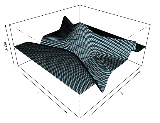
Figure 2. Plot of the function $(x,y)\mapsto\ell_{H}(x,y)$.

Our second main result is the following Berry-Esseen type bound for the random walk $x+S_{n}$ conditioned to stay in the half-line $\mathbb{R}_{+}$.

Theorem 1.4.

Assume that $\mathbb{E}(X_{1})=0$, $\mathbb{E}(X^{2}_{1})=\sigma^{2}>0$ and that there exists $\delta>0$ such that $\mathbb{E}(|X_{1}|^{2+\delta})<\infty.$ Then, there exists a constant $c>0$ such that, for any $n\geqslant 1$, $u\geqslant 0$ and $x\in\mathbb{R}$,

$$\Bigg{|}\mathbb{P}\Bigg{(}\frac{x+S_{n}}{\sigma\sqrt{n}}\leqslant u,\tau_{x}>n\Bigg{)}-\frac{V(x)L\left(\frac{x}{\sigma\sqrt{n}}\right)}{\sigma\sqrt{n}}\int_{0}^{u}\ell_{H}\left(\frac{x}{\sigma\sqrt{n}},y\right)dy\Bigg{|}\leqslant c\frac{R_{n}(\delta,x)}{\sqrt{n}},$$ (1.26)

where $R_{n}(\delta,x)$ is defined by (1.13).

For the proof we refer to Section 4. As a direct consequence of Theorem 1.4 and of Corollary 1.2, we obtain the following generalization of the central limit theorem to conditioned random walks.

Corollary 1.5.

Assume conditions of Theorem 1.4. For any $a\in\operatorname{supp}V$, it holds

$$\lim_{n\to\infty}\sup_{x\geqslant a}\sup_{u\geqslant 0}\Bigg{|}\mathbb{P}\Bigg{(}\frac{x+S_{n}}{\sigma\sqrt{n}}\leqslant u\bigg{|}\tau_{x}>n\Bigg{)}-\int_{0}^{u}\ell_{H}\left(\frac{x}{\sigma\sqrt{n}},y\right)dy\Bigg{|}=0.$$ (1.27)

In particular, as $V(0)>0$, (1.27) holds true with $a=0$.

On the $\sqrt{n}$-scale the approximation (1.27) can be reformulated as follows: uniformly over $u\geqslant 0$ and $t\in[0,\infty)$,

$$\lim_{n\to\infty}\mathbb{P}\Bigg{(}t+\frac{S_{n}}{\sigma\sqrt{n}}\leqslant u\bigg{|}\tau_{t\sigma\sqrt{n}}>n\Bigg{)}=\mathscr{L}_{H}\left(t,u\right):=\int_{0}^{u}\ell_{H}(t,y)dy,$$

where, for any $t\in[0,\infty)$ fixed, $u\mapsto\mathscr{L}_{H}\left(t,u\right)$ is the probability distribution with density $y\mapsto\ell_{H}(t,y)$ on $\mathbb{R}_{+}$. In particular, for $t=0$, by (1.24), we have that, uniformly for $u\geqslant 0$,

$$\lim_{n\to\infty}\mathbb{P}\Bigg{(}\frac{S_{n}}{\sigma\sqrt{n}}\leqslant u\bigg{|}\tau_{0}>n\Bigg{)}=\Phi^{+}(u):=\int_{0}^{u}\phi^{+}(y)dy,$$

where $\Phi^{+}$ is the Rayleigh distribution function.

As in the case of probability $\mathbb{P}\left(\tau_{x}>n\right)$, we shall analyse the scenarios when $x$ is close to the origin and away from the origin on the $\sqrt{n}$-scale.

B1. First we consider the case when $\frac{x}{\sqrt{n}}\to 0$. Using the approximation of $\ell_{H}(x,\cdot)$ by the Rayleigh law given in (1.24) and Lemma 2.5, from Theorem 1.4 we can deduce that, there exists a constant $c>0$ such that, for any sequence $\alpha_{n}\to 0$ as $n\to\infty$, for any $n\geqslant 1$, $u\geqslant 0$ and $x\in\mathbb{R}$ satisfying $\frac{|x|}{\sqrt{n}}\leqslant\alpha_{n}$,

$$\Bigg{|}\mathbb{P}\Bigg{(}\frac{x+S_{n}}{\sigma\sqrt{n}}\leqslant u,\tau_{x}>n\Bigg{)}-\frac{2V(x)}{\sigma\sqrt{2\pi n}}\int_{0}^{u}\phi^{+}(y)dy\Bigg{|}\leqslant c\frac{V(x)}{\sqrt{n}}\alpha_{n}+c\frac{R_{n}(\delta,x)}{\sqrt{n}}.$$ (1.28)

In particular, for any $\varepsilon>0$ and $a\in\operatorname{supp}V$, from (1.28) we have as $n\to\infty$, uniformly in $u\geqslant\varepsilon$ and $x\in[a,\infty)$ satisfying $\frac{|x|}{\sqrt{n}}\leqslant\alpha_{n}$,

$$\mathbb{P}\Bigg{(}\frac{x+S_{n}}{\sigma\sqrt{n}}\leqslant u,\tau_{x}>n\Bigg{)}\sim\frac{2V(x)}{\sigma\sqrt{2\pi n}}\int_{0}^{u}\phi^{+}(y)dy.$$ (1.29)

B2. Let $x=t\sigma\sqrt{n}$, where $t>0$. Taking into account (1.19) and Lemma 2.10, from (1.26) we get the following rate of convergence:

$$\left|\mathbb{P}\left(\frac{x+S_{n}}{\sigma\sqrt{n}}\leqslant u,\tau_{x}>n\right)-\int_{0}^{u}\psi\left(t,y\right)dy\right|$$

$$\qquad\qquad\leqslant c\left(n^{-\delta/2}t^{-\delta}H\left(t\right)+n^{-\frac{1}{2}-\frac{\delta}{4}}+L(t)n^{-\frac{\delta}{4(3+\delta)}}\log n\right).$$ (1.30)

Borovkov [5, Theorem 6] obtained precise asymptotics of any order of the persistence probability $\mathbb{P}\left(\tau_{x}>n\right)$ and of the large deviation probability $\mathbb{P}\big{(}\frac{x+S_{n}}{\sigma\sqrt{n}}>u,\tau_{x}>n\big{)}$. However, the results in [5] do not apply when $x$ is fixed and are established under much stronger conditions than ours, namely that $X_{1}$ has an exponential moment and that the distribution of $X_{1}$ has an absolutely continuous component.

We end this section by giving an alternative expression for the main term in Theorem 1.4. Consider the function $\ell_{h}$ defined as follows: for any $x\in\mathbb{R}$,

$$\ell_{h}(x,y)=\frac{\psi(x,y)}{h(x)},\quad y\in\mathbb{R},$$ (1.31)

where $h(x)=x$ is the so called profile harmonic function. For $x=0$ the function $\ell_{h}$ is defined by continuity, i.e. for any $y\in\mathbb{R}$,

$$\ell_{h}(0,y):=\lim_{x\to 0}\ell_{h}(x,y)=L(0)\phi^{+}(y).$$ (1.32)

Moreover, for any $x\in\mathbb{R}$,

$$L(x)=\int_{\mathbb{R}_{+}}\ell_{h}(x,y)dy.$$ (1.33)

With these notation, one can rewrite the main term of (1.26) as

$$V(x)L\left(\frac{x}{\sigma\sqrt{n}}\right)\int_{0}^{u}\ell_{H}\left(\frac{x}{\sigma\sqrt{n}},y\right)dy=V(x)\int_{0}^{u}\ell_{h}\left(\frac{x}{\sigma\sqrt{n}},y\right)dy.$$

2. Preliminary statements

2.1. Properties of the heat kernel

Let $\left(B_{t}\right)_{t\geqslant 0}$ be a standard Brownian motion on the probability space $\left(\Omega,\mathscr{F},\mathbb{P}\right).$ For any $x\geqslant 0$, define the exit time

$$\tau_{x}^{\sigma B}=\inf\left\{t\geqslant 0:x+\sigma B_{t}<0\right\}.$$

The following well known formulas are due to Levy [29] (Theorem 42.I, pp.194-195).

Lemma 2.1.

For any $x\geqslant 0$, $n\geqslant 1$ and $0\leqslant a<b\leqslant\infty$, it holds

$$\mathbb{P}\left(x+\sigma B_{n}\in\left[a,b\right],\tau_{x}^{\sigma B}>n\right)=\frac{1}{\sigma\sqrt{n}}\int_{a}^{b}\psi\left(\frac{x}{\sigma\sqrt{n}},\frac{y}{\sigma\sqrt{n}}\right)dy.$$

In particular, by taking $a=0$ and $b=\infty$, for any $x\geqslant 0$ and $n\geqslant 1$,

$$\mathbb{P}\left(\tau_{x}^{\sigma B}>n\right)=2\Phi\left(\frac{x}{\sigma\sqrt{n}}\right)-1=\frac{2}{\sigma\sqrt{2\pi n}}\int_{0}^{x}e^{-\frac{s^{2}}{2\sigma^{2}n}}ds.$$

When $\sigma=1$ and $n=1$, we have, for $x\geqslant 0$,

$$H(x)=\mathbb{P}\left(\tau_{x}^{B}>1\right)=2\Phi\left(x\right)-1=\frac{2}{\sqrt{2\pi}}\int_{0}^{x}e^{-\frac{s^{2}}{2}}ds.$$ (2.1)

Lemma 2.2.

For any $x\geqslant 0$ and $\varepsilon\geqslant 0$, we have

$$H(x(1+\varepsilon))\leqslant H(x)(1+\varepsilon)$$ (2.2)

and

$$H(x(1-\varepsilon))\geqslant H(x)(1-\varepsilon).$$ (2.3)

Proof.

Since $H(0)=0$, the first inequality (2.2) is a consequence of the concavity of the map $x\mapsto H(x)$ for $x\in\mathbb{R}_{+}$. Similarly, the second inequality (2.3) follows from the convexity of the map $x\mapsto H(x)$ for $x\in\mathbb{R}_{-}$. ∎

We now establish the important Lipschitz property of the function $L$, which is crucial in the proof of Theorem 1.1.

Lemma 2.3.

There exists a constant $c>0$ such that for any $x,x^{\prime}\in\mathbb{R}$,

$$\left|\frac{L(x^{\prime})}{L(x)}-1\right|\leqslant c|x^{\prime}-x|.$$

Proof.

For any $x,x^{\prime}\in\mathbb{R}$, denote $a=x^{\prime}-x$ and

$$R(x,a):=\frac{L(x+a)-L(x)}{aL(x)}.$$

An elementary analysis which is performed below shows that $\sup_{x,a\in\mathbb{R}}|R(x,a)|\leqslant c$, for some positive constant $c>0$. Therefore, the result follows.

Since the function $L$ is even, we have $R(x,a)=-R(-x,-a)$ for any $x,a\in\mathbb{R}$. Therefore, it suffices to show that $|R(x,a)|\leqslant c$ in the following five cases:

Case (i): $x\geqslant 0$ and $a\geqslant 0$. By the definition of $H$ and $L$ (cf. (2.1) and (1.11)), we have

$$I(x,a):=\frac{H(x+a)-H(x)}{aL(x)}=\frac{\frac{1}{a}\int_{x}^{x+a}e^{-\frac{s^{2}}{2}}ds}{\frac{1}{x}\int_{0}^{x}e^{-\frac{s^{2}}{2}}ds}.$$

Since the function $s\mapsto e^{-\frac{s^{2}}{2}}$ is decreasing on $\mathbb{R}_{+}$, for any $x\geqslant 0$ and $a\geqslant 0$, we have $e^{-\frac{(x+a)^{2}}{2}}\leqslant\frac{1}{a}\int_{x}^{x+a}e^{-\frac{s^{2}}{2}}ds\leqslant e^{-\frac{x^{2}}{2}}$ and $e^{-\frac{x^{2}}{2}}\leqslant\frac{1}{x}\int_{0}^{x}e^{-\frac{s^{2}}{2}}ds\leqslant 1$, so that $e^{-\frac{(x+a)^{2}}{2}}\leqslant I(x,a)\leqslant 1$. Hence, for any $x\geqslant 0$ and $a\geqslant 0$,

$$\frac{1}{x+a}\left(e^{-\frac{(x+a)^{2}}{2}}-1\right)\leqslant R(x,a)=\frac{1}{x+a}\left(I(x,a)-1\right)\leqslant 0.$$

Let $f(t)=\frac{1}{t}(e^{-\frac{t^{2}}{2}}-1)$, $t\geqslant 0$. For $t\geqslant 1$, we have $f(t)\geqslant-\frac{1}{t}\geqslant-1$. For $t\in[0,1)$, using the inequality $e^{-\frac{t^{2}}{2}}\geqslant 1-\frac{t^{2}}{2}$, we get $f(t)\geqslant-\frac{t}{2}\geqslant-\frac{1}{2}$. Therefore, $\frac{1}{x+a}(e^{-\frac{(x+a)^{2}}{2}}-1)\geqslant-1$ for all $x,a\geqslant 0$ and we have proved that $\sup_{x,a\geqslant 0}|R(x,a)|\leqslant 1$.

Case (ii): $2\geqslant x\geqslant 0$ and $-2\leqslant a<0$. By the mean value theorem, there exists $\tilde{x}\in(x+a,x)$ such that

$$L(x+a)-L(x)=aL^{\prime}(\tilde{x})=a\frac{L^{\prime}(\tilde{x})}{L(\tilde{x})}L(\tilde{x}).$$

Since $L(x)=\frac{H(x)}{x}$, we have

$$\frac{L^{\prime}(x)}{L(x)}=-\frac{1}{x}+\frac{H^{\prime}(x)}{H(x)}=-\frac{1}{x}+\frac{e^{-\frac{x^{2}}{2}}}{\int_{0}^{x}e^{-\frac{s^{2}}{2}}ds}.$$

By L’Hôpital’s rule, it holds that $\lim_{x\to 0}\frac{L^{\prime}(x)}{L(x)}=0$. Hence the function $x\mapsto\frac{L^{\prime}(x)}{L(x)}$ is continuous on $\mathbb{R}$ and bounded on $[-2,2]$, so $|\frac{L^{\prime}(\tilde{x})}{L(\tilde{x})}|\leqslant c$ for some constant $c$. As the function $L$ is continuous and strictly positive on $[-2,2]$, there exists a constant $c>0$ such that $L(\tilde{x})\leqslant cL(x)$ for all $x,\tilde{x}\in[-2,2]$. Therefore, there exists a constant $c^{\prime}>0$ such that $|L(x+a)-L(x)|\leqslant c^{\prime}|a|L(x)$ for all $2\geqslant x\geqslant 0$ and $-2\leqslant a<0$, as desired.

Case (iii): $x\geqslant 1$, $a<0$ and $x+a\geqslant 1$. Since the function $s\mapsto e^{-\frac{s^{2}}{2}}$ is decreasing on $\mathbb{R}_{+}$, we have $\frac{1}{x}\int_{0}^{x}e^{-\frac{s^{2}}{2}}ds\leqslant\frac{1}{x+a}\int_{0}^{x+a}e^{-\frac{s^{2}}{2}}ds$. Hence,

$$I(x,a)=\frac{\frac{1}{a}\int_{x}^{x+a}e^{-\frac{s^{2}}{2}}ds}{\frac{1}{x}\int_{0}^{x}e^{-\frac{s^{2}}{2}}ds}=\frac{\frac{1}{-a}\int_{x+a}^{x}e^{-\frac{s^{2}}{2}}ds}{\frac{1}{x}\int_{0}^{x}e^{-\frac{s^{2}}{2}}ds}\leqslant 1,$$ (2.4)

so that $R(x,a)=\frac{1}{x+a}\left(I(x,a)-1\right)\leqslant 0$. For the lower bound, since $\frac{1}{-a}\int_{x+a}^{x}e^{-\frac{s^{2}}{2}}ds\geqslant e^{-\frac{x^{2}}{2}}$ and $\frac{1}{x}\int_{0}^{x}e^{-\frac{s^{2}}{2}}ds\leqslant 1$, we have $I(x,a)\geqslant e^{-\frac{x^{2}}{2}}$. Taking into account that $x+a\geqslant 1$, we get

$$R(x,a)\geqslant\frac{1}{x+a}\left(e^{-\frac{x^{2}}{2}}-1\right)\geqslant-\frac{1}{x+a}\geqslant-1.$$

Therefore, $|R(x,a)|\leqslant 1$ for all $x\geqslant 1$ and $a<0$ with $x+a\geqslant 1$.

Case (iv): $x\geqslant 1$, $a<0$ and $x+a\in[0,1]$. As in (2.4), we have $R(x,a)\leqslant 0$ in this case, so it remains to give a lower bound for $R(x,a)$. Since $\frac{1}{-a}\int_{x+a}^{x}e^{-\frac{s^{2}}{2}}ds\geqslant e^{-\frac{x^{2}}{2}}$ and $\frac{1}{x}\int_{0}^{x}e^{-\frac{s^{2}}{2}}ds\leqslant 1$, we get

$$R(x,a)=\frac{1}{x+a}\left(\frac{\frac{1}{-a}\int_{x+a}^{x}e^{-\frac{s^{2}}{2}}ds}{\frac{1}{x}\int_{0}^{x}e^{-\frac{s^{2}}{2}}ds}-1\right)\geqslant\frac{1}{x+a}\left(e^{-\frac{x^{2}}{2}}-1\right).$$

Now we further consider two cases: $x+2a>0$ and $x+2a\leqslant 0$. If $x+2a>0$, we have $\frac{1}{x+a}\leqslant\frac{2}{x}$. Since in case (i) we have shown that $f(t)=\frac{1}{t}(e^{-\frac{t^{2}}{2}}-1)\geqslant-1$ for all $t\in\mathbb{R}_{+}$, we get

$$R(x,a)\geqslant\frac{1}{x+a}\left(e^{-\frac{x^{2}}{2}}-1\right)\geqslant\frac{2}{x}\left(e^{-\frac{x^{2}}{2}}-1\right)\geqslant-2.$$

If $x+2a\leqslant 0$, we have $\frac{x}{a}\geqslant-2$. Since $a<0$ and $x+a\geqslant 0$, it holds that $\frac{1}{x}\leqslant\frac{1}{-a}$ and hence

$$\frac{1}{-a}\int_{x+a}^{x}e^{-\frac{s^{2}}{2}}ds-\frac{1}{x}\int_{0}^{x}e^{-\frac{s^{2}}{2}}ds\geqslant\frac{1}{-a}\left(\int_{x+a}^{x}e^{-\frac{s^{2}}{2}}ds-\int_{0}^{x}e^{-\frac{s^{2}}{2}}ds\right)=\frac{1}{a}\int_{0}^{x+a}e^{-\frac{s^{2}}{2}}ds.$$

Note that $\frac{1}{x+a}\int_{0}^{x+a}e^{-\frac{s^{2}}{2}}ds\leqslant 1$, and $\int_{0}^{x}e^{-\frac{s^{2}}{2}}ds\geqslant\int_{0}^{1}e^{-\frac{s^{2}}{2}}ds\geqslant e^{-1/2}$ since $x\geqslant 1$. Therefore, taking into account that $\frac{x}{a}\geqslant-2$, we obtain

$$R(x,a)=\frac{1}{x+a}\frac{\frac{1}{-a}\int_{x+a}^{x}e^{-\frac{s^{2}}{2}}ds-\frac{1}{x}\int_{0}^{x}e^{-\frac{s^{2}}{2}}ds}{\frac{1}{x}\int_{0}^{x}e^{-\frac{s^{2}}{2}}ds} \geqslant\frac{1}{x+a}\frac{\frac{1}{a}\int_{0}^{x+a}e^{-\frac{s^{2}}{2}}ds}{\frac{1}{x}\int_{0}^{x}e^{-\frac{s^{2}}{2}}ds}$$

$$=\frac{x}{a}\frac{\frac{1}{x+a}\int_{0}^{x+a}e^{-\frac{s^{2}}{2}}ds}{\int_{0}^{x}e^{-\frac{s^{2}}{2}}ds}\geqslant-2e^{-1/2}.$$

Combining the above estimates, we conclude that $|R(x,a)|\leqslant 2$ for all $x\geqslant 1$ and $a<0$ with $x+a\in[0,1]$.

Case (v): $1\geqslant x>0$ and $a<-2$. In this case, we have $e^{-\frac{(x+a)^{2}}{2}}\leqslant\frac{1}{-a}\int_{x+a}^{x}e^{-\frac{s^{2}}{2}}ds\leqslant 1$ and $e^{-\frac{x^{2}}{2}}\leqslant\frac{1}{x}\int_{0}^{x}e^{-\frac{s^{2}}{2}}ds\leqslant 1$, so that

$$I(x,a)=\frac{\frac{1}{-a}\int_{x+a}^{x}e^{-\frac{s^{2}}{2}}ds}{\frac{1}{x}\int_{0}^{x}e^{-\frac{s^{2}}{2}}ds}-1\in\left[e^{-\frac{(x+a)^{2}}{2}}-1,e^{\frac{x^{2}}{2}}-1\right].$$

Since $x+a<0$, we get

$$R(x,a)=\frac{1}{x+a}\left(\frac{\frac{1}{-a}\int_{x+a}^{x}e^{-\frac{s^{2}}{2}}ds}{\frac{1}{x}\int_{0}^{x}e^{-\frac{s^{2}}{2}}ds}-1\right)\in\left[\frac{1}{x+a}\left(e^{\frac{x^{2}}{2}}-1\right),\frac{1}{x+a}\left(e^{-\frac{(x+a)^{2}}{2}}-1\right)\right].$$

As $1\geqslant x>0$ and $x+a<-1$, we have $\frac{1}{x+a}>-1$ and $e^{\frac{x^{2}}{2}}-1\geqslant e^{1/2}-1>1$. Hence $\frac{1}{x+a}(e^{\frac{x^{2}}{2}}-1)>-1$. Since we have shown in case (i) that $\frac{1}{t}(e^{-\frac{t^{2}}{2}}-1)\geqslant-1$ for all $t\geqslant 0$, we get $\frac{1}{x+a}(e^{-\frac{(x+a)^{2}}{2}}-1)\leqslant 1$. Therefore, $|R(x,a)|\leqslant 1$ for all $1\geqslant x>0$ and $a<-2$. ∎

Lemma 2.4.

For any $a\in\operatorname{supp}V$, there exist constants $c_{1},c_{2}>0$ such that, for any $n\geqslant 1$ and $x\in[a,\infty)$,

$$c_{1}\leqslant V(x)L\left(\frac{x}{\sigma\sqrt{n}}\right)\leqslant c_{2}\sqrt{n}.$$ (2.5)

Proof.

For $x\in[a,\sigma\sqrt{n}]$, we have $V(x)\geqslant V(a)>0$ and $L(x)\geqslant\min\{L(\frac{a}{\sigma\sqrt{n}}),L(1)\}\geqslant c^{\prime}_{1}>0$ for any $n\geqslant 1$. For $x>\sigma\sqrt{n}$, by (1.11) we have $V(x)L(\frac{x}{\sigma\sqrt{n}})=\frac{V(x)}{x}\sigma\sqrt{n}H(\frac{x}{\sigma\sqrt{n}})\geqslant c\sigma\sqrt{n}H(1)>c^{\prime\prime}_{1}>0,$ for any $n\geqslant 1.$ Therefore the lower bound in (2.5) holds with $c_{1}=\max\{c^{\prime}_{1},c^{\prime\prime}_{2}\}$. For the upper bound, when $x\in[a,\sigma\sqrt{n})$, since $V(x)\leqslant c^{\prime}_{2}\sqrt{n}$, we have $V(x)L(\frac{x}{\sigma\sqrt{n}})\leqslant c^{\prime}_{2}\sqrt{n}L(1)$. When $x\geqslant\sigma\sqrt{n}$, since $\frac{V(x)}{x}\sim 1$, we have $V(x)L(\frac{x}{\sigma\sqrt{n}})=\frac{V(x)}{x}\sigma\sqrt{n}H(\frac{x}{\sigma\sqrt{n}})\leqslant c^{\prime\prime}_{2}\sqrt{n}$. Thus, the upper bound in (2.5) follows. ∎

The following lemma will play a key role in the proof of Theorem 1.4.

Lemma 2.5.

There exists a constant $c>0$ such that, for any $x,x^{\prime}\in\mathbb{R}$ with $|x-x^{\prime}|\leqslant 1$, and any measurable set $D\subseteq\mathbb{R}$,

$$\left|\int_{D}\ell_{h}(x^{\prime},y)dy-\int_{D}\ell_{h}(x,y)dy\right|\leqslant cL(x)|x-x^{\prime}|.$$

Proof.

By the definition of $\ell_{H}$ and $\ell_{h}$ (cf. (1.23) and (1.31)), we have $\ell_{h}(x,y)=L(x)\ell_{H}(x,y)$, which implies that, for any $x\in\mathbb{R}$ and $a\in[-1,1]$,

$$\int_{D}\left(\ell_{h}(x+a,y)-\ell_{h}(x,y)\right)dy$$

$$=L(x+a)\int_{D}\ell_{H}(x+a,y)dy-L(x)\int_{D}\ell_{H}(x,y)dy$$

$$=L(x+a)\int_{D}\left(\ell_{H}(x+a,y)-\ell_{H}(x,y)\right)dy+\left(L(x+a)-L(x)\right)\int_{D}\ell_{H}(x,y)dy$$

$$=:J_{1}+J_{2}.$$ (2.6)

For the first term, there exists $\theta\in(0,1)$ such that

$$\ell_{H}(x+a,y)-\ell_{H}(x,y)=a\frac{d}{dx^{\prime}}\ell_{H}(x^{\prime},y)\Big{|}_{x^{\prime}=x+\theta a}.$$ (2.7)

By the definition of $\ell_{H}$ (cf. (1.23) and (1.21)), we have

$$\frac{d}{dx}\ell_{H}(x,y)=\frac{1}{H(x)^{2}}\Big{[}H(x)\Big{(}\phi^{\prime}(x-y)-\phi^{\prime}(x+y)\Big{)}-2\phi(x)\Big{(}\phi(x-y)-\phi(x+y)\Big{)}\Big{]}.$$ (2.8)

First assume that $|x|>1$. Then, from (2.8), it follows that

$$\Big{|}\frac{d}{dx}\ell_{H}(x,y)\Big{|} \leqslant\frac{1}{|H(x)|}\Big{(}|\phi^{\prime}(x-y)|+|\phi^{\prime}(x+y)|\Big{)}+\frac{2\phi(x)}{H(x)^{2}}\Big{(}|\phi(y+x)|+|\phi(y-x)|\Big{)}$$

$$\leqslant c\Big{(}|\phi^{\prime}(x-y)|+|\phi^{\prime}(x+y)|+|\phi(y+x)|+|\phi(y-x)|\Big{)}.$$

Denote $g_{0}(t)=\sup_{|z|\leqslant 1}\phi(t+z)$ and $g_{1}(t)=\sup_{|z|\leqslant 1}\phi^{\prime}(t+z)$ and remark that $\int_{\mathbb{R}}g_{k}(t)dt<\infty$ for $k=0,1.$ Then there exists $c>0$ such that for any $y\in\mathbb{R}$ and $a\in[-1,1]$,

$$\Big{|}\frac{d}{dx^{\prime}}\ell_{H}(x^{\prime},y)\Big{|}_{x^{\prime}=x+\theta a}\Big{|} \leqslant c\Big{(}g_{1}(x-y)+g_{1}(x+y)+g_{0}(y+x)|+g_{0}(y-x)\Big{)}.$$

Substituting this into (2.7) and using Lemma 2.3, we get

$$|J_{1}| \leqslant caL(x+a)\int_{D}\Big{(}g_{1}(x-y)+g_{1}(x+y)+g_{0}(y+x)|+g_{0}(y-x)\Big{)}dy$$

$$\leqslant ca(1+a)L(x)\left(\int_{0}^{\infty}g_{1}(y)dy+\int_{0}^{\infty}g_{0}(y)dy\right)$$

$$\leqslant caL(x).$$

Secondly, assume that $|x|\leqslant 1$. We rewrite (2.8) as follows:

$$\frac{d}{dx}\ell_{H}(x,y) =\frac{1}{H(x)^{2}}\Big{[}\left(xH(x)+2\phi(x)\right)\left(\phi(y+x)-\phi(y-x)\right)$$

$$\qquad\qquad\qquad+yH(x)\left(\phi(y+x)+\phi(y-x)\right)\Big{]}.$$ (2.9)

By Taylor’s expansion, there exist $\theta_{1},\theta_{2},\theta_{3}\in(0,1)$ such that

$$\phi(y+x) =\phi(y)+x\phi^{\prime}(y)+\frac{x^{2}}{2}\phi^{\prime\prime}(y+\theta_{1}x)=\phi(y)-xy\phi(y)+\frac{x^{2}}{2}\phi^{\prime\prime}(y+\theta_{1}x),$$

$$\phi(y-x) =\phi(y)-x\phi^{\prime}(y)+\frac{x^{2}}{2}\phi^{\prime\prime}(y+\theta_{2}x)=\phi(y)+xy\phi(y)+\frac{x^{2}}{2}\phi^{\prime\prime}(y+\theta_{2}x)$$

and

$$H(x) =2x\phi(x)+x^{2}\phi^{\prime}(\theta_{3}x).$$

Hence,

$$\frac{d}{dx}\ell_{H}(x,y) =\frac{1}{H(x)^{2}}\Bigg{[}\left(xH(x)+2\phi(x)\right)\left(-2xy\phi(y)+\frac{x^{2}}{2}\phi^{\prime\prime}(y+\theta_{1}x)-\frac{x^{2}}{2}\phi^{\prime\prime}(y+\theta_{2}x)\right)$$

$$\quad+y\left(2x\phi(x)+x^{2}\phi^{\prime}(\theta_{3}x)\right)\left(2\phi(y)+\frac{x^{2}}{2}\phi^{\prime\prime}(y+\theta_{1}x)+\frac{x^{2}}{2}\phi^{\prime\prime}(y+\theta_{2}x)\right)\Bigg{]}$$

$$=\frac{1}{H(x)^{2}}\Bigg{[}\left(xH(x)+2\phi(x)\right)\left(\frac{x^{2}}{2}\phi^{\prime\prime}(y+\theta_{1}x)-\frac{x^{2}}{2}\phi^{\prime\prime}(y+\theta_{2}x)\right)$$

$$\quad+y\left(2x\phi(x)+x^{2}\phi^{\prime}(\theta_{3}x)\right)\left(\frac{x^{2}}{2}\phi^{\prime\prime}(y+\theta_{1}x)+\frac{x^{2}}{2}\phi^{\prime\prime}(y+\theta_{2}x)\right)\Bigg{]}.$$

Denote $g_{2}(t)=\sup_{|z|\leqslant 1}\phi^{\prime\prime}(t+z)$ so that $\int_{\mathbb{R}}g_{2}(t)dt<\infty$. Then, taking into account that $xL(x)=H(x)$, we obtain

$$\left|\frac{d}{dx}\ell_{H}(x,y)\right| \leqslant\frac{1}{H(x)^{2}}\Bigg{[}\left(x^{2}L(x)+2\phi(x)\right)x^{2}g_{2}(y)+2x^{2}|y|\phi(y)|H(x)|$$

$$\quad+|y|\left(2|x|\phi(x)+x^{2}g_{1}(0)\right)x^{2}g_{2}(y)+2|y|x^{2}\phi(y)g_{1}(0)\Bigg{]}$$

$$=\frac{x^{2}}{H(x)^{2}}\left(x^{2}L(x)+2\phi(x)\right)g_{2}(y)+2|y|\phi(y)|H(x)|\frac{x^{2}}{H(x)^{2}}$$

$$\quad+\left(2|x|\phi(x)+x^{2}g_{1}(0)\right)\frac{x^{2}}{H(x)^{2}}|y|g_{2}(y)+2|y|\phi(y)g_{1}(0)$$

$$\leqslant c\Big{(}g_{2}(y)+|y|\phi(y)+|y|g_{2}(y)\Big{)}.$$

Using (2.7) and the last bound, we have

$$\int_{D}\left|\ell_{H}(x+a,y)-\ell_{H}(x,y)\right|dy\leqslant c|a|\int_{\mathbb{R}}\left[g_{2}(y)+|y|\phi(y)+|y|g_{2}(y)\right]dy\leqslant c|a|.$$

Therefore, for the first term in the right-hand side of (2.1) we have

$$|J_{1}|\leqslant c|a|L(x+a)\leqslant c|a|L(x)(1+|a|)\leqslant c|a|L(x).$$

For the second term in in the right-hand side of (2.1), by Lemma 2.3,

$$|J_{2}|\leqslant c|a|L(x)\int_{\mathbb{R}}|\ell_{H}(x,y)|dy\leqslant 2c|a|L(x).$$

This concludes the proof of the lemma. ∎

2.2. Technical results

The purpose of this subsection is to state several auxiliary results that will be used to establish the conditioned integral limit theorems (Theorems 1.1 and 1.4). Throughout this section, unless otherwise specified, we assume the following conditions: $\mathbb{E}(X_{1})=0$, $\mathbb{E}(X^{2}_{1})=\sigma^{2}>0$ and there exists a constant $\delta>0$ such that $\mathbb{E}(|X_{1}|^{2+\delta})<\infty.$

The following functional central limit theorem, proved by Sakhanenko [33] (see also [27]), provides a way to couple out the random walk with the Brownian motion.

Lemma 2.6.

There exists a construction of the random walk $(S_{n})_{n\geqslant 0}$ on the initial probability space together with a continuous time Brownian motion $(B_{t})_{t\geqslant 0}$ such that for any $s>0$ and $n\geqslant 1$,

$$\mathbb{P}\left(\sup_{0\leqslant t\leqslant 1}\left|S_{[nt]}-\sigma B_{nt}\right|>\sigma n^{1/2-s}\right)\leqslant\frac{c_{\delta,s}}{n^{\frac{\delta}{2}-(2+\delta)s}},$$

where $c_{\delta,s}$ is a constant depending on $\delta$ and $s$.

Note that the assertion of the lemma becomes effective when $s\in(0,\frac{\delta}{2(2+\delta)})$.

The following lemma is elementary.

Lemma 2.7.

For any $r\in(0,2+\delta]$, there exists a constant $c>0$ such that for any $n\geqslant 1$,

$$\mathbb{E}\left(\max_{1\leqslant k\leqslant n}|S_{k}|^{r}\right)\leqslant cn^{r/2}.$$

Proof.

By Rosenthal’s inequality, for any $s\in[2,2+\delta]$, there exists a constant $c>0$ such that for any $n\geqslant 1$,

$$\mathbb{E}\left(\max_{1\leqslant k\leqslant n}|S_{k}|^{s}\right)\leqslant c\sum_{i=1}^{n}\mathbb{E}\left(|X_{i}|^{s}\right)+c\left[\sum_{i=1}^{n}\mathbb{E}\left(|X_{i}|^{2}\right)\right]^{s/2}\leqslant cn^{s/2}.$$

Using this with $s=2$ and Hölder’s inequality, we get that, for $r\in(0,2+\delta]$, there exists a constant $c>0$ such that for any $n\geqslant 1$,

$$\mathbb{E}\left(\max_{1\leqslant k\leqslant n}|S_{k}|^{r}\right)\leqslant\left[\mathbb{E}\left(\max_{1\leqslant k\leqslant n}|S_{k}|^{2}\right)\right]^{r/2}\leqslant cn^{r/2},$$

completing the proof of the lemma. ∎

We shall need the following Fuk-Nagaev inequality (cf. [19]).

Lemma 2.8.

Assume that $\mathbb{E}X_{i}=0$ and $\mathbb{E}(X_{i}^{2})=\sigma^{2}>0$. Then, for any $n\geqslant 1$ and $x,y>0$,

$$\mathbb{P}\left(|S_{n}|>x,\max_{1\leqslant i\leqslant n}|X_{i}|\leqslant y\right)\leqslant 2e^{x/y}\left(\frac{n\sigma^{2}}{xy}\right)^{x/y}.$$

The following lemma, adapted from [21, Lemma 5.8], is a consequence of the central limit theorem.

Lemma 2.9.

There exists a constant $c>0$ such that, for any $M\geqslant 1$ and $n\geqslant 1$,

$$\sup_{x\in\mathbb{R}}\mathbb{P}\left(\sup_{1\leqslant k\leqslant n}|x+S_{k}|\leqslant M\right)\leqslant ce^{-\frac{n}{2M^{2}}}.$$

Proof.

Let $m=[\rho^{-2}M^{2}]$ and $K=\left[n/m\right]$, where $\rho>0$ will be chosen later. It is easy to see that, for any $t\in\mathbb{R}$,

$$\mathbb{P}\left(\max_{1\leqslant k\leqslant n}\left|t+S_{k}\right|\leqslant M\right)\leqslant\mathbb{P}\left(\max_{1\leqslant k\leqslant K}\left|t+S_{km}\right|\leqslant M\right).$$ (2.10)

Using the independence of the random variables $(X_{k})$, it follows that

$$\mathbb{P}\left(\max_{1\leqslant k\leqslant K}\left|x+S_{km}\right|\leqslant M\right)\leqslant\mathbb{P}\left(\max_{1\leqslant k\leqslant K-1}\left|x+S_{km}\right|\leqslant M\right)\sup_{x^{\prime}\in\mathbb{R}}\mathbb{P}\left(\left|x^{\prime}+S_{m}\right|\leqslant M\right),$$

from which iterating, we get

$$\mathbb{P}\left(\max_{1\leqslant k\leqslant K}\left|t+S_{km}\right|\leqslant M\right)\leqslant\left(\sup_{t^{\prime}\in\mathbb{R}}\mathbb{P}\left(\left|x^{\prime}+S_{m}\right|\leqslant M\right)\right)^{K}.$$ (2.11)

By the central limit theorem, there exist a sequence $r_{m}\to 0$ as $m\to\infty$ and a constant $q\in(0,1)$ such that, for any $x^{\prime}\in\mathbb{R}$ and $m\geqslant 1$,

$$\mathbb{P}\left(\left|x^{\prime}+S_{m}\right|\leqslant M\right)=\mathbb{P}\left(\frac{S_{m}}{\sqrt{m}}\in\left[\frac{-M-x^{\prime}}{\sqrt{m}},\frac{M-t^{\prime}}{\sqrt{m}}\right]\right)\leqslant\int_{\frac{-M-x^{\prime}}{\sqrt{m}}}^{\frac{M-x^{\prime}}{\sqrt{m}}}\phi_{\sigma^{2}}(u)du+r_{m}\leqslant q,$$

where for the last inequality we take $\rho>0$ sufficiently small and $m$ sufficiently large so that $\frac{2M}{\sqrt{m}}+r_{m}\leqslant 4\rho+r_{m}\leqslant q$. The assertion of the lemma follows from (2.10) and (2.11). ∎

The following bound is due to Rogozin ([32, Corollary 4]).

Lemma 2.10.

There exists $c>0$ such that, for any $x\geqslant 1$,

$$0\leqslant\frac{V(x)}{x}-1\leqslant cx^{-\delta}.$$ (2.12)

We continue with the following preliminary bound for the expectation of the random walk $(x+S_{n})_{n\geqslant 1}$ killed at the exit time $\tau_{x}$.

Lemma 2.11.

There exists a constant $c>0$ such that for any $n\geqslant 1$ and $x\in\mathbb{R}$,

$$\max\{x,0\}\leqslant\mathbb{E}\left(x+S_{n};\tau_{x}>n\right)\leqslant V(x)=-\mathbb{E}(S_{\tau_{x}}).$$ (2.13)

Proof.

By the optional stopping theorem, for any $x\in\mathbb{R}$, we get

$$\mathbb{E}(x+S_{n};\tau_{x}>n) =\mathbb{E}(x+S_{n})-\mathbb{E}(x+S_{n};1\leqslant\tau_{x}\leqslant n)$$

$$=x-\mathbb{E}(x+S_{\tau_{x}};1\leqslant\tau_{x}\leqslant n).$$ (2.14)

Since, on the event $\{1\leqslant\tau_{x}\leqslant n\}$ it holds $-(x+S_{\tau_{x}})\geqslant 0$, we get

$$0\leqslant-\mathbb{E}(x+S_{\tau_{x}};1\leqslant\tau_{x}\leqslant n)\leqslant-\mathbb{E}(x+S_{\tau_{x}})=-x-\mathbb{E}(S_{\tau_{x}})=-x+V(x),$$

where the last equality holds due to (1.4). Substituting this into (2.2) completes the proof of the lemma. ∎

We will need the following elementary inequality from [21, Lemma 5.10].

Lemma 2.12.

For any $x\in\mathbb{R}$ and any random variable $Z$,

$$\mathbb{E}^{1/2}\left(\left(x+Z\right)^{2};x+Z\geqslant 0\right)\leqslant\max\{x,0\}+\mathbb{E}^{1/2}(Z^{2}).$$

Proof.

If $x\leqslant 0$, we have $Z\geqslant-x\geqslant 0$ since $x+Z\geqslant 0$. Hence $(x+Z)^{2}\leqslant Z^{2}$ and the assertion follows. If $x>0$, using $\mathbb{E}Z\leqslant\mathbb{E}^{1/2}(Z^{2})$, we get $x^{2}+2x\mathbb{E}Z+\mathbb{E}Z^{2}\leqslant x^{2}+2x\mathbb{E}^{1/2}(Z^{2})+\mathbb{E}Z^{2},$ from which the assertion follows. ∎

3. Proofs for the persistence probability

In this section, we give a proof of Theorem 1.1 by using the bounds shown in Section 2.1 and the functional central limit theorem (Lemma 2.6). All over this section we assume that $\mathbb{E}(X_{1})=0$, $\mathbb{E}(X^{2}_{1})=\sigma^{2}>0$ and that there exists $\delta>0$ such that $\mathbb{E}(|X_{1}|^{2+\delta})<\infty.$

3.1. Auxiliary results

Let $\varepsilon\in[0,\frac{1}{2}]$. For any $x\in\mathbb{R}$ and $n\geqslant 1$, consider the first time when the random variable $|x+S_{k}|$ exceeds the level $M_{n}:=n^{1/2-\varepsilon}$:

$$\nu_{n}=\nu_{n,\varepsilon}=\inf\left\{k\geqslant 1:|x+S_{k}|>M_{n}\right\}.$$ (3.1)

The following lemma gives the tail behavior of $\nu_{n}$. Let $N_{n}=N_{n}^{\varepsilon}:=[\gamma n^{1-2\varepsilon}\log n]$, where $\gamma>0$ is chosen to be a sufficiently large constant.

Lemma 3.1.

For any $\gamma>0$, there exists a constant $c>0$ such that for any $n\geqslant 1$, $x\in\mathbb{R}$ and $\varepsilon\in[0,\frac{1}{2}]$,

$$\mathbb{P}\left(\nu_{n}>N_{n}\right)=\mathbb{P}\left(\nu_{n}>[\gamma n^{1-2\varepsilon}\log n]\right)\leqslant cn^{-\gamma/2}.$$

Proof.

It suffices to consider the case $n\geqslant 2$. Since for $\varepsilon\in[0,1/2]$, we have $M_{n}=n^{1/2-\varepsilon}\geqslant 1$. Using Lemma 2.9, we get

$$\mathbb{P}\left(\nu_{n}\geqslant N_{n}\right) =\mathbb{P}\left(\sup_{1\leqslant k\leqslant N_{n}}|x+S_{k}|\leqslant M_{n}\right)$$

$$\leqslant c\exp\left(-\frac{N_{n}}{2M_{n}^{2}}\right)=c\exp\left(-\frac{[\gamma n^{1-2\varepsilon}\log n]}{2n^{1-2\varepsilon}}\right)\leqslant cn^{-\gamma/2},$$

which proves the assertion of the lemma. ∎

For any $x\in\mathbb{R}$ and $n\geqslant 1$, set

$$E_{x,n,\varepsilon}=\mathbb{E}\left(x+S_{\nu_{n,\varepsilon}};\tau_{x}>\nu_{n,\varepsilon},\nu_{n,\varepsilon}\leqslant N_{n}^{\varepsilon}\right).$$

The following lemma will be used repeatedly in the subsequent analysis to establish Theorems 1.1 and 1.4. It demonstrates that $E_{x,n,\varepsilon}$ is well approximated by the harmonic function $V$.

Lemma 3.2.

For any $\varepsilon\in[0,\frac{1}{2}]$ and $\gamma>0$, there exists a constant $c>0$ such that for any $n\geqslant 1$ and $x\in\mathbb{R}$,

$$E_{x,n,\varepsilon}\leqslant V(x)\leqslant\left(1+n^{-(1/2-\varepsilon)\delta}\right)E_{x,n,\varepsilon}+c\frac{1+V(x)}{n^{\gamma/8}}.$$ (3.2)

Proof.

Let $n\geqslant 1$, $x\in\mathbb{R}$ and $\varepsilon\in[0,\frac{1}{2}]$. By (1.6), the sequence $\big{(}V(x+S_{n})\mathds{1}_{\{\tau_{x}>n\}}\big{)}_{n\geqslant 1}$ is a martingale with respect to the filtration $\mathscr{F}_{n}=\sigma(X_{1},\ldots,X_{n})$. Therefore, by the optional stopping theorem,

$$V(x) =\mathbb{E}\left(V(x+S_{n});\tau_{x}>n\right)$$

$$=\mathbb{E}\left(V(x+S_{n});\tau_{x}>n,\nu_{n}\leqslant N_{n}\right)+\mathbb{E}\left(V(x+S_{n});\tau_{x}>n,\nu_{n}>N_{n}\right)$$

$$=\mathbb{E}\left(V(x+S_{\nu_{n}});\tau_{x}>\nu_{n},\nu_{n}\leqslant N_{n}\right)+\mathbb{E}\left(V(x+S_{n});\tau_{x}>n,\nu_{n}>N_{n}\right).$$ (3.3)

By Lemma 2.11, we have $V(x)\geqslant\max\{x,0\}$ for $x\in\mathbb{R}$, which implies that the last term in the right-hand side of (3.1) is non-negative. Therefore, from (3.1) and the fact that $V(x+S_{\nu_{n}})\geqslant x+S_{\nu_{n}}$ on the event $\{\tau_{x}>\nu_{n}\}$, we get that, for any $x\in\mathbb{R}$,

$$V(x)\geqslant\mathbb{E}\left(V(x+S_{\nu_{n}});\tau_{x}>\nu_{n},\nu_{n}\leqslant N_{n}\right)\geqslant\mathbb{E}\left(x+S_{\nu_{n}};\tau_{x}>\nu_{n},\nu_{n}\leqslant N_{n}\right)=E_{x,n,\varepsilon},$$

which proves the left-hand side bound of (3.2). For the right-hand side bound, since $x^{\prime}=x+S_{\nu_{n}}\geqslant n^{1/2-\varepsilon}$ on the event $\{\tau_{x}>\nu_{n}\}$, using Lemma 2.10, we get

$$V(x+S_{\nu_{n}})\leqslant\left(1+c(x+S_{\nu_{n}})^{-\delta}\right)(x+S_{\nu_{n}})\leqslant\left(1+n^{-(1/2-\varepsilon)\delta}\right)(x+S_{\nu_{n}}).$$

It follows that

$$\mathbb{E}\left(V(x+S_{\nu_{n}});\tau_{x}>\nu_{n},\nu_{n}\leqslant N_{n}\right) \leqslant\left(1+n^{-(1/2-\varepsilon)\delta}\right)\mathbb{E}\left(x+S_{\nu_{n}};\tau_{x}>\nu_{n},\nu_{n}\leqslant N_{n}\right)$$

$$=\left(1+n^{-(1/2-\varepsilon)\delta}\right)E_{x,n,\varepsilon}.$$ (3.4)

Combining (3.1) and (3.1), we have, for any $n\geqslant 1$ and $x\in\mathbb{R}$,

$$V(x)\leqslant\left(1+n^{-(1/2-\varepsilon)\delta}\right)E_{x,n,\varepsilon}+\mathbb{E}\left(V(x+S_{n});\tau_{x}>n,\nu_{n}>N_{n}\right).$$ (3.5)

By the Cauchy-Schwarz inequality, the bound $V(x^{\prime})\leqslant c(1+x^{\prime})$ for $x^{\prime}\geqslant 0$ (cf. Lemma 2.10) and Lemma 3.1, we get that for any $\varepsilon\in[0,1/2]$ and $\gamma>0$, there exists a constant $c>0$ such that, for any $n\geqslant 1$ and $x\in\mathbb{R}$,

$$\mathbb{E}\left(V(x+S_{n});\tau_{x}>n,\nu_{n}>N_{n}\right) \leqslant c(V(x)+n^{1/2})\mathbb{P}^{1/2}\left(\nu_{n}>N_{n}\right)$$

$$\leqslant c(1+V(x))n^{-\gamma/8}.$$ (3.6)

Combining (3.5) and (3.1), we obtain that for any $\varepsilon\in[0,1/2]$ and $\gamma>0$, there exists a constant $c>0$ such that, for any $n\geqslant 1$ and $x\in\mathbb{R}$,

$$V(x)\leqslant\left(1+n^{-(1/2-\varepsilon)\delta}\right)E_{x,n,\varepsilon}+c(1+V(x))n^{-\gamma/8}.$$

This finishes the proof of (3.2). ∎

Using Lemmas 3.1 and 3.2, we show the following upper bound for the persistence probability $\mathbb{P}\left(\tau_{x}>n\right)$, which will be applied in the proof of Lemma 3.5.

Lemma 3.3.

There exists a constant $c>0$ such that for any $n\geqslant 1$ and $x\in\mathbb{R}$,

$$\mathbb{P}\left(\tau_{x}>n\right)\leqslant c\frac{1+V(x)L\left(\frac{x}{\sigma\sqrt{n}}\right)}{n^{1/2}}.$$

Proof.

Using Lemma 3.1 with $\varepsilon=0$ and the fact that $x+S_{\nu_{n,0}}\geqslant n^{1/2}$ on the event $\{\tau_{x}>\nu_{n,0}\}$, we get that, for any $\gamma>0$, there exists a constant $c>0$ such that for any $n\geqslant 1$ and $x\in\mathbb{R}$,

$$\mathbb{P}(\tau_{x}>n) =\mathbb{P}\left(\tau_{x}>n,\nu_{n,0}\leqslant N_{n}^{0}\right)+\mathbb{P}\left(\tau_{x}>n,\nu_{n,0}>N_{n}^{0}\right)$$

$$\leqslant\frac{1}{n^{1/2}}\mathbb{E}\left(x+S_{\nu_{n,0}};\tau_{x}>\nu_{n,0},\nu_{n,0}\leqslant N_{n}^{0}\right)+cn^{-\gamma/2}.$$

Using Lemma 3.2, we have

$$E_{x,n,0}=\mathbb{E}\left(x+S_{\nu_{n,0}};\tau_{x}>\nu_{n,0},\nu_{n,0}\leqslant N_{n}^{0}\right)\leqslant V(x).$$

Therefore, choosing $\gamma>0$ large enough, there exists a constant $c$ such that, for any $n\geqslant 1$ and $x\in\mathbb{R}$,

$$\mathbb{P}\left(\tau_{x}>n\right)\leqslant c\frac{1+V(x)}{n^{1/2}}.$$

From Lemma 2.3, there exists $c>0$ such that $L\left(\frac{x}{\sigma\sqrt{n}}\right)\geqslant cL(0)$ for any $n\geqslant 1$ and $0\leqslant x\leqslant\frac{\sigma}{2}n^{1/2}$. Therefore, for any $0\leqslant x\leqslant\frac{\sigma}{2}n^{1/2}$,

$$\mathbb{P}\left(\tau_{x}>n\right)\leqslant c\frac{1+V(x)}{n^{1/2}}\leqslant c\frac{1+V(x)L\left(\frac{x}{\sigma\sqrt{n}}\right)}{n^{1/2}}.$$ (3.7)

For $x>\frac{\sigma}{2}n^{1/2}$, we have, with some constant $c>0,$

$$\mathbb{P}(\tau_{x}>n)\leqslant cH\left(\frac{x}{\sigma\sqrt{n}}\right)=c\frac{x}{\sqrt{n}}L\left(\frac{x}{\sigma\sqrt{n}}\right)\leqslant c\frac{V(x)L\left(\frac{x}{\sigma\sqrt{n}}\right)}{\sqrt{n}}.$$

For $x<0$, since $\mathbb{P}\left(\tau_{x}>n\right)\leqslant\mathbb{P}\left(\tau_{0}>n\right)$, using (3.7), it holds that

$$\mathbb{P}\left(\tau_{x}>n\right)\leqslant\mathbb{P}\left(\tau_{0}>n\right)\leqslant\frac{c_{1}}{n^{1/2}}\leqslant c_{1}\frac{1+V(x)L\left(\frac{x}{\sigma\sqrt{n}}\right)}{n^{1/2}}.$$ (3.8)

This ends the proof of the lemma. ∎

As a consequence of Lemmas 2.3 and 2.6, the next result provides relative error estimates for the probability $\mathbb{P}(\tau_{x}>n)$ with the Dirichlet heat kernel $H$ defined by (1.8).

Lemma 3.4.

1. There exists a constant $c>0$ such that, for any $n\geqslant 1$, $a\in(0,1]$ and $x\geqslant a\sigma\sqrt{n}$,

$$\left|\frac{\mathbb{P}\left(\tau_{x}>n\right)}{H\left(\frac{x}{\sigma\sqrt{n}}\right)}-1\right|\leqslant\frac{c}{a}n^{-\frac{\delta}{2(3+\delta)}}.$$ (3.9)

2. Moreover, if $\delta\geqslant 1$, then there exists a constant $c>0$ such that, for any $n\geqslant 1$, $a\in(0,1]$ and $x\geqslant a\sigma\sqrt{n}$,

$$\left|\frac{\mathbb{P}\left(\tau_{x}>n\right)}{H\left(\frac{x}{\sigma\sqrt{n}}\right)}-1\right|\leqslant\frac{c}{a\sqrt{n}}.$$ (3.10)

Proof.

By Lemma 2.6, for any $s>0$, there exists $c=c_{s,\delta}>0$ such that, for any $n\geqslant 1$ and $x\in\mathbb{R}$,

$$H\left(\frac{x}{\sigma\sqrt{n}}-n^{-s}\right)-\frac{c}{n^{\frac{\delta}{2}-s(2+\delta)}}\leqslant\mathbb{P}(\tau_{x}>n)\leqslant H\left(\frac{x}{\sigma\sqrt{n}}+n^{-s}\right)+\frac{c}{n^{\frac{\delta}{2}-s(2+\delta)}}.$$ (3.11)

Using Lemma 2.3, we have

$$H\left(\frac{x}{\sigma\sqrt{n}}+n^{-s}\right) =\left(\frac{x}{\sigma\sqrt{n}}+n^{-s}\right)L\left(\frac{x}{\sigma\sqrt{n}}+n^{-s}\right)$$

$$\leqslant\left(\frac{x}{\sigma\sqrt{n}}+n^{-s}\right)L\left(\frac{x}{\sigma\sqrt{n}}\right)\left(1+cn^{-s}\right)$$

$$\leqslant H\left(\frac{x}{\sigma\sqrt{n}}\right)\left(1+cn^{-s}\right)+L\left(\frac{x}{\sigma\sqrt{n}}\right)n^{-s}\left(1+cn^{-s}\right).$$

Taking into account that $x\geqslant a\sigma\sqrt{n}$, we get

$$H\left(\frac{x}{\sigma\sqrt{n}}+n^{-s}\right) \leqslant H\left(\frac{x}{\sigma\sqrt{n}}\right)\left(1+cn^{-s}\right)+cH\left(\frac{x}{\sigma\sqrt{n}}\right)\frac{1}{an^{s}}$$

$$\leqslant H\left(\frac{x}{\sigma\sqrt{n}}\right)\left(1+c^{\prime}\frac{1}{an^{s}}\right).$$ (3.12)

Since $H$ is increasing on $\mathbb{R}_{+}$, there exists $c>0$ such that for any $a\in(0,1]$ and $x\geqslant a\sigma\sqrt{n}$, we have

$$H\left(\frac{x}{\sigma\sqrt{n}}\right)\geqslant H(a)\geqslant ca.$$ (3.13)

From (3.11) and (3.1), by choosing $s=\frac{\delta}{2(3+\delta)}$, we get the following upper bound:

$$\frac{\mathbb{P}\left(\tau_{x}>n\right)}{H\left(\frac{x}{\sigma\sqrt{n}}\right)}-1\leqslant\frac{c}{a}n^{-\frac{\delta}{2(3+\delta)}}.$$

The lower bound can be obtained in the same way, so that (3.9) holds.

Now we show the second assertion (3.10). As a consequence of Nagaev’s bound (1.9), there exists $c>0$ such that for any $n\geqslant 1$ and $x\geqslant 0$,

$$\left|\frac{\mathbb{P}\left(\tau_{x}>n\right)}{H\left(\frac{x}{\sigma\sqrt{n}}\right)}-1\right|\leqslant\frac{c}{\sqrt{n}H\left(\frac{x}{\sigma\sqrt{n}}\right)}.$$

Since $x\geqslant a\sigma\sqrt{n}$, the bound (3.10) follows from (3.13). ∎

3.2. Proof of Theorem 1.1

It suffices to consider the case $n\geqslant 2$. Recall that $M_{n}=n^{1/2-\varepsilon}$ and $N_{n}=[\gamma n^{1-2\varepsilon}\log n]$, where $\varepsilon\in(0,\frac{1}{2})$ and $\gamma>0$ will be chosen to be a sufficiently large constant. Using the Markov property, we have for any $n\geqslant 1$ and $x\in\mathbb{R}$,

$$\mathbb{P}\left(\tau_{x}>n\right)=J_{1}+J_{2},$$ (3.14)

where

$$J_{1}=\mathbb{P}\left(\tau_{x}>n,\nu_{n}>N_{n}\right),$$

$$J_{2}=\mathbb{P}\left(\tau_{x}>n,\nu_{n}\leqslant N_{n}\right)=\sum_{k=1}^{N_{n}}\int_{M_{n}}^{\infty}\mathbb{P}(\tau_{x^{\prime}}>n-k)\mathbb{P}\left(x+S_{k}\in dx^{\prime},\tau_{x}>k,\nu_{n}=k\right).$$

Bound of $J_{1}$. By Lemma 3.1, for any $\gamma>0$, there exists a constant $c>0$ such that for any $n\geqslant 1$, $x\in\mathbb{R}$ and $\varepsilon\in[0,\frac{1}{2}]$,

$$J_{1}\leqslant\mathbb{P}\left(\nu_{n}>N_{n}\right)\leqslant cn^{-\gamma/2}.$$ (3.15)

Upper bound of $J_{2}$. Let $k\in[1,N_{n}]$ and $x^{\prime}\geqslant M_{n}=n^{1/2-\varepsilon}$. Using Lemma 3.4 with $a=n^{-\varepsilon}$, we get

$$\mathbb{P}(\tau_{x^{\prime}}>n-k)\leqslant H\left(\frac{x^{\prime}}{\sigma\sqrt{n-k}}\right)\left(1+cn^{\varepsilon}r_{n,\delta}\right),$$ (3.16)

where $r_{n,\delta}=n^{-\frac{\delta}{2(3+\delta)}}$ is the remainder term in (3.9). Substituting (3.16) into $J_{2}$ gives

$$J_{2}\leqslant\left(1+cn^{\varepsilon}r_{n,\delta}\right)\sum_{k=1}^{N_{n}}\mathbb{E}\left(H\left(\frac{x+S_{k}}{\sigma\sqrt{n-k}}\right);\tau_{x}>k,\nu_{n}=k\right).$$ (3.17)

Since for any $k\in[1,N_{n}]$,

$$\frac{\sqrt{n}}{\sqrt{n-k}}=1+\frac{k}{\sqrt{n-k}(\sqrt{n}+\sqrt{n-k})}\leqslant 1+c\frac{k}{n}\leqslant 1+c\frac{N_{n}}{n},$$ (3.18)

by Lemma 2.2, we have that for any $x^{\prime}\geqslant 0$,

$$H\left(\frac{x^{\prime}}{\sigma\sqrt{n-k}}\right)\leqslant H\left(\frac{x^{\prime}}{\sigma\sqrt{n}}\right)\left(1+c\frac{N_{n}}{n}\right).$$

Combining this with (3.17), we obtain

$$J_{2} \leqslant\left(1+cn^{\varepsilon}r_{n,\delta}\right)\left(1+c\frac{N_{n}}{n}\right)\sum_{k=1}^{N_{n}}\mathbb{E}\left(H\left(\frac{x+S_{k}}{\sigma\sqrt{n}}\right);\tau_{x}>k,\nu_{n}=k\right)$$

$$\leqslant\left(1+cn^{\varepsilon}r_{n,\delta}+c\frac{N_{n}}{n}\right)\sum_{k=1}^{N_{n}}\mathbb{E}\left(H\left(\frac{x+S_{k}}{\sigma\sqrt{n}}\right);\tau_{x}>k,\nu_{n}=k\right)$$

$$=\left(1+cn^{\varepsilon}r_{n,\delta}+c\frac{N_{n}}{n}\right)(J_{3}+J_{4}),$$ (3.19)

where

$$J_{3}=\sum_{k=1}^{N_{n}}\mathbb{E}\left(H\left(\frac{x+S_{k}}{\sigma\sqrt{n}}\right);\frac{|S_{k}|}{\sigma\sqrt{n}}>\alpha n^{-\varepsilon}\log n,\tau_{x}>k,\nu_{n}=k\right)$$ (3.20)

and

$$J_{4}=\sum_{k=1}^{N_{n}}\mathbb{E}\left(H\left(\frac{x+S_{k}}{\sigma\sqrt{n}}\right);\frac{|S_{k}|}{\sigma\sqrt{n}}\leqslant\alpha n^{-\varepsilon}\log n,\tau_{x}>k,\nu_{n}=k\right),$$ (3.21)

with the constant $\alpha>0$ whose value will be chosen below.

The remainder of this section focuses on deriving upper and lower bounds for $J_{3}$ and $J_{4}$. Specifically, we will demonstrate that $J_{3}$ is negligible, whereas $J_{4}$ constitutes the dominant term.

Lemma 3.5.

For any $\varepsilon\in(0,\frac{1}{2}]$, there exists a constant $c=c_{\varepsilon}>0$ such that, for any $n\geqslant 2$ and $x\in\mathbb{R}$,

$$J_{3}\leqslant c\frac{1+V(x)L\left(\frac{x}{\sigma\sqrt{n}}\right)}{n^{\frac{1}{2}+\frac{\delta}{2}-\delta\varepsilon}}(\log n)^{3/2}.$$

Proof.

We will use the Fuk-Nagaev inequality (Lemma 2.8). Let

$$\eta_{n}=\inf\left\{k\geqslant 1:\frac{|X_{k}|}{\sigma\sqrt{n}}\geqslant\alpha n^{-\varepsilon}\right\},$$ (3.22)

where $\alpha>0$ is given in (3.20). By (3.20), we have that for $n\geqslant 2$,

$$J_{3} =\sum_{k=1}^{N_{n}}\mathbb{E}\left(H\left(\frac{x+S_{k}}{\sigma\sqrt{n}}\right);\frac{|S_{k}|}{\sigma\sqrt{n}}>\alpha n^{-\varepsilon}\log n,\tau_{x}>k,\eta_{n}>k,\nu_{n}=k\right)$$

$$\quad+\sum_{k=1}^{N_{n}}\mathbb{E}\left(H\left(\frac{x+S_{k}}{\sigma\sqrt{n}}\right);\frac{|S_{k}|}{\sigma\sqrt{n}}>\alpha n^{-\varepsilon}\log n,\tau_{x}>k,\eta_{n}\leqslant k,\nu_{n}=k\right)$$

$$=:J_{31}+J_{32}.$$ (3.23)

For the first term $J_{31}$, since $H\leqslant 1$, we have

$$J_{31}\leqslant\sum_{k=1}^{N_{n}}\mathbb{P}\left(\frac{|S_{k}|}{\sigma\sqrt{n}}>\alpha n^{-\varepsilon}\log n,\eta_{n}>k\right).$$ (3.24)

Applying the Fuk-Nagaev inequality (Lemma 2.8) with $x=\alpha\sigma n^{1/2-\varepsilon}\log n$ and $y=\alpha\sigma n^{1/2-\varepsilon}$, we get that for any $1\leqslant k\leqslant N_{n}$,

$$\mathbb{P}\left(\frac{|S_{k}|}{\sqrt{n}}>\alpha\sigma n^{-\varepsilon}\log n,\eta_{n}>k\right)$$

$$=\mathbb{P}\left(|S_{k}|>\alpha\sigma n^{1/2-\varepsilon}\log n,\max_{1\leqslant j\leqslant k}|X_{j}|\leqslant\alpha\sigma n^{1/2-\varepsilon}\right)$$

$$\leqslant 2\exp\left\{\frac{n^{1/2-\varepsilon}\log n}{n^{1/2-\varepsilon}}\right\}\left(\frac{\gamma n^{1-2\varepsilon}\log n}{\alpha^{2}n^{1/2-\varepsilon}n^{1/2-\varepsilon}\log n}\right)^{\frac{n^{1/2-\varepsilon}\log n}{n^{1/2-\varepsilon}}}$$

$$\leqslant 2n\left(\frac{\gamma}{\alpha^{2}}\right)^{\log n}=2n^{-(\log(\alpha^{2}/\gamma)-1)}\leqslant 2n^{-\log\alpha},$$ (3.25)

where in the last inequality we choose $\alpha\geqslant\gamma$. From (3.24) and (3.2), we get the following upper bound for the first term $J_{31}$: for any $\alpha\geqslant e^{2}$ and $n\geqslant 2$,

$$J_{31}\leqslant\sum_{k=1}^{N_{n}}\mathbb{P}\left(\frac{|S_{k}|}{\sigma\sqrt{n}}>\alpha n^{-\varepsilon}\log n,\eta_{n}>k\right)\leqslant 2N_{n}n^{-\log\alpha}\leqslant c_{\gamma}n^{-\frac{1}{2}\log\alpha}.$$ (3.26)

We proceed to handle the second term $J_{32}$. Taking into account that $H(x^{\prime})=x^{\prime}L(x^{\prime})$ for $x^{\prime}\in\mathbb{R}$, by Lemma 2.3, we get

$$J_{32} \leqslant\sum_{k=1}^{N_{n}}\mathbb{E}\left(\frac{x+S_{k}}{\sigma\sqrt{n}}L\left(\frac{x+S_{k}}{\sigma\sqrt{n}}\right);\tau_{x}>k,\eta_{n}\leqslant k,\nu_{n}=k\right)$$

$$\leqslant L\left(\frac{x}{\sigma\sqrt{n}}\right)\sum_{k=1}^{N_{n}}\mathbb{E}\left(\frac{x+S_{k}}{\sigma\sqrt{n}}\left(1+c\frac{|S_{k}|}{\sqrt{n}}\right);\tau_{x}>k,\eta_{n}\leqslant k,\nu_{n}=k\right).$$

By (2.13), we have $x+S_{k}\leqslant V(x)+|S_{k}|$. It follows that

$$J_{32} \leqslant c\frac{V(x)L\left(\frac{x}{\sigma\sqrt{n}}\right)}{\sqrt{n}}\sum_{k=1}^{N_{n}}\mathbb{P}\left(\tau_{x}>k,\eta_{n}\leqslant k,\nu_{n}=k\right)$$

$$\quad+cL\left(\frac{x}{\sigma\sqrt{n}}\right)\left(1+\frac{V(x)}{\sqrt{n}}\right)\sum_{k=1}^{N_{n}}\mathbb{E}\left(\frac{|S_{k}|}{\sqrt{n}};\tau_{x}>k,\eta_{n}\leqslant k,\nu_{n}=k\right)$$

$$\quad+cL\left(\frac{x}{\sigma\sqrt{n}}\right)\sum_{k=1}^{N_{n}}\mathbb{E}\left(\frac{S_{k}^{2}}{n};\tau_{x}>k,\eta_{n}\leqslant k,\nu_{n}=k\right)$$

$$=:G_{1}+G_{2}+G_{3}.$$ (3.27)

Bound of $G_{1}$. By the definition of $\eta_{n}$ (cf. (3.22)) and the fact that $N_{n}=[\gamma n^{1-2\varepsilon}\log n]$, it holds that for any $\varepsilon\in(0,\frac{1}{2}]$,

$$\mathbb{P}\left(\eta_{n}\leqslant N_{n}\right)\leqslant N_{n}\mathbb{P}\left(|X_{1}|>\alpha\sigma n^{1/2-\varepsilon}\right)\leqslant c\frac{n^{1-2\varepsilon}\mathbb{E}|X_{1}|^{2+\delta}}{n^{(1/2-\varepsilon)(2+\delta)}}\log n\leqslant\frac{c}{n^{\frac{\delta}{2}-\delta\varepsilon}}\log n.$$ (3.28)

Using (3.28) gives the following bound for $G_{1}$:

$$G_{1}\leqslant c\frac{V(x)L\left(\frac{x}{\sigma\sqrt{n}}\right)}{\sqrt{n}}\mathbb{P}\left(\eta_{n}\leqslant N_{n}\right)\leqslant c\frac{V(x)L\left(\frac{x}{\sigma\sqrt{n}}\right)}{n^{\frac{1}{2}+\frac{\delta}{2}-\delta\varepsilon}}\log n.$$ (3.29)

Bound of $G_{2}$. Since $|S_{\nu_{n}}|\leqslant|S_{\nu_{n}}-S_{k}|+|X_{k}|+|S_{k-1}|$, we write

$$\sum_{k=1}^{N_{n}}\mathbb{E}\left(\frac{|S_{k}|}{\sqrt{n}};\tau_{x}>k,\eta_{n}\leqslant k,\nu_{n}=k\right)$$

$$=\mathbb{E}\left(\frac{|S_{\nu_{n}}|}{\sqrt{n}};\tau_{x}>\nu_{n},\eta_{n}\leqslant\nu_{n}\leqslant N_{n}\right)$$

$$\leqslant\sum_{k=1}^{N_{n}}\mathbb{E}\left(\frac{|S_{\nu_{n}}|}{\sqrt{n}};\tau_{x}>k,k\leqslant\nu_{n}\leqslant N_{n},\eta_{n}=k\right)$$

$$\leqslant\frac{1}{\sqrt{n}}\sum_{k=1}^{N_{n}}\mathbb{E}\left(|S_{\nu_{n}}-S_{k}|;\tau_{x}>k,k\leqslant\nu_{n}\leqslant N_{n},\eta_{n}=k\right)$$

$$\quad+\frac{1}{\sqrt{n}}\sum_{k=1}^{N_{n}}\mathbb{E}\left(|X_{k}|;\tau_{x}>k,k\leqslant\nu_{n}\leqslant N_{n},\eta_{n}=k\right)$$

$$\quad+\frac{1}{\sqrt{n}}\sum_{k=1}^{N_{n}}\mathbb{E}\left(|S_{k-1}|;\tau_{x}>k,k\leqslant\nu_{n}\leqslant N_{n},\eta_{n}=k\right)$$

$$=:F_{1}+F_{2}+F_{3}.$$ (3.30)

For $F_{1}$, we have

$$F_{1} \leqslant\frac{1}{\sqrt{n}}\sum_{k=1}^{N_{n}}\mathbb{E}\left(\max_{l\in[k,N_{n}]}|S_{l}-S_{k}|;\tau_{x}>k,\eta_{n}=k\right)$$

$$\leqslant\frac{1}{\sqrt{n}}\sum_{k=1}^{N_{n}}\mathbb{E}\left(\max_{l\in[k,N_{n}]}|S_{l}-S_{k}|;\tau_{x}>k-1,\eta_{n}=k\right)$$

$$=\frac{1}{\sqrt{n}}\sum_{k=1}^{N_{n}}\mathbb{E}\left(\max_{l\in[k,N_{n}]}|S_{l}-S_{k}|\right)\mathbb{P}\left(\tau_{x}>k-1\right)\mathbb{P}\left(\eta_{n}=k\right)$$

$$\leqslant\frac{c\sqrt{N_{n}}}{\sqrt{n}}\sum_{k=1}^{N_{n}}\mathbb{P}\left(\tau_{x}>k-1\right)\mathbb{P}\left(\eta_{n}=k\right),$$ (3.31)

where for the last line we used Burkholder’s inequality (see Lemma 2.7):

$$\mathbb{E}\left(\max_{l\in[k,N_{n}]}|S_{l}-S_{k}|\right)\leqslant c\sqrt{N_{n}}.$$

By the definition of $\eta_{n}$ (cf. (3.22)), and using the fact that $\mathbb{E}(|X_{1}|^{2+\delta})<\infty$, we have

$$\mathbb{P}\left(\eta_{n}=k\right)=\mathbb{P}\left(|X_{k}|>\alpha\sigma n^{1/2-\varepsilon}\right)\leqslant\frac{c}{n^{(1/2-\varepsilon)(2+\delta)}}=\frac{c}{n^{1+\frac{\delta}{2}-2\varepsilon-\varepsilon\delta}}.$$ (3.32)

Since the function $t\mapsto L(t)$ is decreasing on $\mathbb{R}_{+}$, we have $L\left(\frac{x}{\sigma\sqrt{k}}\right)\leqslant L\left(\frac{x}{\sigma\sqrt{n}}\right)$ for any $1\leqslant k\leqslant n$ and $x\geqslant 0$. Therefore, by Lemma 3.3, there exists a constant $c>0$ such that, for any $1\leqslant k\leqslant n$ and $x\geqslant 0$,

$$\mathbb{P}\left(\tau_{x}>k\right)\leqslant c\frac{1+V(x)L\left(\frac{x}{\sigma\sqrt{k}}\right)}{k^{1/2}}\leqslant c\frac{1+V(x)L\left(\frac{x}{\sigma\sqrt{n}}\right)}{k^{1/2}}.$$ (3.33)

For $x<0$, in view of (3.8), we have $\mathbb{P}\left(\tau_{x}>k\right)\leqslant\mathbb{P}\left(\tau_{0}>k\right)\leqslant\frac{c}{k^{1/2}}\leqslant c\frac{1+V(x)L(\frac{x}{\sigma\sqrt{n}})}{k^{1/2}}$, which proves that (3.33) holds for all $x\in\mathbb{R}$. Therefore, recalling that $N_{n}=[\gamma n^{1-2\varepsilon}\log n]$, we get

$$\sum_{k=1}^{N_{n}}\mathbb{P}\left(\tau_{x}>k-1\right) \leqslant 1+c\left(1+V(x)L\left(\frac{x}{\sigma\sqrt{n}}\right)\right)\sum_{k=1}^{N_{n}}\frac{1}{k^{1/2}}$$

$$\leqslant 1+c\left(1+V(x)L\left(\frac{x}{\sigma\sqrt{n}}\right)\right)N_{n}^{\frac{1}{2}}$$

$$\leqslant c(n^{1-2\varepsilon}\log n)^{\frac{1}{2}}\left(1+V(x)L\left(\frac{x}{\sigma\sqrt{n}}\right)\right).$$ (3.34)

Combining (3.32) and (3.2), we get

$$\sum_{k=1}^{N_{n}}\mathbb{P}\left(\tau_{x}>k-1\right)\mathbb{P}\left(\eta_{n}=k\right)\leqslant c\frac{\sqrt{\log n}}{n^{\frac{1}{2}+\frac{\delta}{2}-\varepsilon-\varepsilon\delta}}\left(1+V(x)L\left(\frac{x}{\sigma\sqrt{n}}\right)\right).$$ (3.35)

From (3.2) and (3.35), we obtain the following bound for $F_{1}$:

$$F_{1} \leqslant\frac{c}{\sqrt{n}}(n^{1-2\varepsilon}\log n)^{1/2}\frac{\sqrt{\log n}}{n^{\frac{1}{2}+\frac{\delta}{2}-\varepsilon-\varepsilon\delta}}\left(1+V(x)L\left(\frac{x}{\sigma\sqrt{n}}\right)\right)$$

$$\leqslant c\frac{\log n}{n^{\frac{1}{2}+\frac{\delta}{2}-\delta\varepsilon}}\left(1+V(x)L\left(\frac{x}{\sigma\sqrt{n}}\right)\right).$$ (3.36)

Now we deal with the term $F_{2}$ defined in (3.2). By independence, we have

$$F_{2} \leqslant\frac{1}{\sqrt{n}}\sum_{k=1}^{N_{n}}\mathbb{E}\left(|X_{k}|;\tau_{x}>k-1,|X_{k}|>\alpha\sigma n^{1/2-\varepsilon}\right)$$

$$=\frac{1}{\sqrt{n}}\mathbb{E}\left(|X_{1}|;|X_{1}|>\alpha\sigma n^{1/2-\varepsilon}\right)\sum_{k=1}^{N_{n}}\mathbb{P}\left(\tau_{x}>k-1\right).$$

Using the condition $\mathbb{E}(|X_{1}|^{2+\delta})<\infty$ and the bound (3.2), we get that, for any $n\geqslant 1$ and $x\in\mathbb{R}$,

$$F_{2} \leqslant\frac{c}{\sqrt{n}}\frac{1}{n^{(1/2-\varepsilon)(1+\delta)}}(n^{1-2\varepsilon}\log n)^{\frac{1}{2}}\left(1+V(x)L\left(\frac{x}{\sigma\sqrt{n}}\right)\right)$$

$$\leqslant\frac{c\sqrt{\log n}}{n^{\frac{1}{2}+\frac{\delta}{2}-\delta\varepsilon}}\left(1+V(x)L\left(\frac{x}{\sigma\sqrt{n}}\right)\right).$$ (3.37)

To handle $F_{3}$ in (3.2), we decompose it into two terms:

$$F_{3} \leqslant\frac{1}{\sqrt{n}}\sum_{k=1}^{N_{n}}\mathbb{E}\left(|S_{k-1}|;|S_{k-1}|>\alpha\sigma n^{1/2-\varepsilon}\log n,\eta_{n}=k\right)$$

$$\quad+\frac{1}{\sqrt{n}}\sum_{k=1}^{N_{n}}\mathbb{E}\left(|S_{k-1}|;|S_{k-1}|\leqslant\alpha\sigma n^{1/2-\varepsilon}\log n,\tau_{x}>k,\eta_{n}=k\right)$$

$$=:F_{31}+F_{32},$$ (3.38)

where $\alpha\geqslant e$ is the same as that in (3.22). For the first term $F_{31}$ in (3.2), using the fact that $|S_{k-1}|\leqslant n^{3/2}$ on the event $\{\eta_{n}=k\}$ for any $1\leqslant k\leqslant N_{n}$, and the bound (3.2), we get

$$F_{31} \leqslant cn\sum_{k=1}^{N_{n}}\mathbb{P}\left(|S_{k-1}|>\alpha\sigma n^{1/2-\varepsilon}\log n,\eta_{n}=k\right)$$

$$\leqslant cn\sum_{k=1}^{N_{n}}\mathbb{P}\left(|S_{k-1}|>\alpha\sigma n^{1/2-\varepsilon}\log n,\max_{1\leqslant j\leqslant k-1}|X_{j}|\leqslant\alpha\sigma n^{1/2-\varepsilon}\right)$$

$$\leqslant cn^{2}n^{-\log\alpha}\leqslant cn^{-\frac{1}{2}\log\alpha},$$ (3.39)

where in the last inequality we take $\alpha\geqslant e^{3}$. For the second term $F_{32}$ in (3.2), using (3.35), we have

$$F_{32} \leqslant cn^{-\varepsilon}\log n\sum_{k=1}^{N_{n}}\mathbb{P}\left(\tau_{x}>k,\eta_{n}=k\right)$$

$$\leqslant cn^{-\varepsilon}\log n\sum_{k=1}^{N_{n}}\mathbb{P}\left(\tau_{x}>k-1\right)\mathbb{P}\left(\eta_{n}=k\right)$$

$$\leqslant cn^{-\varepsilon}\log n\frac{\sqrt{\log n}}{n^{\frac{1}{2}+\frac{\delta}{2}-\varepsilon-\varepsilon\delta}}\left(1+V(x)L\left(\frac{x}{\sigma\sqrt{n}}\right)\right)$$

$$\leqslant c\frac{(\log n)^{3/2}}{n^{\frac{1}{2}+\frac{\delta}{2}-\delta\varepsilon}}\left(1+V(x)L\left(\frac{x}{\sigma\sqrt{n}}\right)\right).$$ (3.40)

Substituting (3.2) and (3.2) into (3.2), and taking $\alpha>0$ to be sufficiently large (e.g. $\log\alpha>1+\delta-2\delta\varepsilon$), we get the following bound for $F_{3}$:

$$F_{3}\leqslant\frac{c(\log n)^{3/2}}{n^{\frac{1}{2}+\frac{\delta}{2}-\delta\varepsilon}}\left(1+V(x)L\left(\frac{x}{\sigma\sqrt{n}}\right)\right).$$ (3.41)

Coming back to estimation of $G_{2}$ from (3.2) and collecting the bounds for $F_{1}$, $F_{2}$, $F_{3}$ from (3.2), (3.2), (3.2) and (3.41), we get that there exists $c=c_{\varepsilon}>0$ such that

$$G_{2} \leqslant cL\left(\frac{x}{\sigma\sqrt{n}}\right)\left(1+\frac{V(x)}{\sqrt{n}}\right)(F_{1}+F_{2}+F_{3})$$

$$\leqslant cL\left(\frac{x}{\sigma\sqrt{n}}\right)\left(1+\frac{V(x)}{\sqrt{n}}\right)\frac{1+V(x)L\left(\frac{x}{\sigma\sqrt{n}}\right)}{n^{\frac{1}{2}+\frac{\delta}{2}-\delta\varepsilon}}(\log n)^{3/2}.$$ (3.42)

Bound of $G_{3}$. The estimate of $G_{3}$ can be obtained by following the same strategy of the proof of $G_{2}$ in (3.2). As in (3.2), using the inequality $S_{\nu_{n}}^{2}\leqslant 3(S_{\nu_{n}}-S_{k})^{2}+3X_{k}^{2}+3S_{k-1}^{2}$, we have

$$\sum_{k=1}^{N_{n}}\mathbb{E}\left(\frac{S_{k}^{2}}{n};\tau_{x}>k,\eta_{n}\leqslant k,\nu_{n}=k\right)$$

$$=\mathbb{E}\left(\frac{S_{\nu_{n}}^{2}}{n};\tau_{x}>\nu_{n},\eta_{n}\leqslant\nu_{n}\leqslant N_{n}\right)$$

$$\leqslant\sum_{k=1}^{N_{n}}\mathbb{E}\left(\frac{S_{\nu_{n}}^{2}}{n};\tau_{x}>k,k\leqslant\nu_{n}\leqslant N_{n},\eta_{n}=k\right)$$

$$\leqslant\frac{3}{n}\sum_{k=1}^{N_{n}}\mathbb{E}\left((S_{\nu_{n}}-S_{k})^{2};\tau_{x}>k,k\leqslant\nu_{n}\leqslant N_{n},\eta_{n}=k\right)$$

$$\quad+\frac{3}{n}\sum_{k=1}^{N_{n}}\mathbb{E}\left(X_{k}^{2};\tau_{x}>k,k\leqslant\nu_{n}\leqslant N_{n},\eta_{n}=k\right)$$

$$\quad+\frac{3}{n}\sum_{k=1}^{N_{n}}\mathbb{E}\left(S_{k-1}^{2};\tau_{x}>k,k\leqslant\nu_{n}\leqslant N_{n},\eta_{n}=k\right)$$

$$=:F^{\prime}_{1}+F^{\prime}_{2}+F^{\prime}_{3}.$$ (3.43)

For $F^{\prime}_{1}$, following the proof of (3.2), using Lemma 2.7 and (3.35), we obtain the following bound for $F^{\prime}_{1}$:

$$F^{\prime}_{1} \leqslant\frac{3}{n}\sum_{k=1}^{N_{n}}\mathbb{E}\left(\max_{l\in[k,N_{n}]}(S_{l}-S_{k})^{2}\right)\mathbb{P}\left(\tau_{x}>k-1\right)\mathbb{P}\left(\eta_{n}=k\right)$$

$$\leqslant c\frac{N_{n}}{n}\sum_{k=1}^{N_{n}}\mathbb{P}\left(\tau_{x}>k-1\right)\mathbb{P}\left(\eta_{n}=k\right)$$

$$\leqslant cn^{-2\varepsilon}\log n\frac{\sqrt{\log n}}{n^{\frac{1}{2}+\frac{\delta}{2}-\varepsilon-\varepsilon\delta}}\left(1+V(x)L\left(\frac{x}{\sigma\sqrt{n}}\right)\right)$$

$$\leqslant c\frac{(\log n)^{3/2}}{n^{\frac{1}{2}+\frac{\delta}{2}+\varepsilon-\delta\varepsilon}}\left(1+V(x)L\left(\frac{x}{\sigma\sqrt{n}}\right)\right).$$ (3.44)

Now we deal with the second term $F^{\prime}_{2}$ in (3.2). By independence, we have

$$F^{\prime}_{2} \leqslant\frac{c}{n}\sum_{k=1}^{N_{n}}\mathbb{E}\left(X_{k}^{2};\tau_{x}>k-1,|X_{k}|>\alpha\sigma n^{1/2-\varepsilon}\right)$$

$$=\frac{c}{n}\mathbb{E}\left(X_{1}^{2};|X_{1}|>\alpha\sigma n^{1/2-\varepsilon}\right)\sum_{k=1}^{N_{n}}\mathbb{P}\left(\tau_{x}>k-1\right).$$

Using the condition $\mathbb{E}(|X_{1}|^{2+\delta})<\infty$ and the bound (3.2), we get the following bound for $F^{\prime}_{2}$:

$$F^{\prime}_{2} \leqslant\frac{c}{n}\frac{1}{n^{(1/2-\varepsilon)\delta}}(n^{1-2\varepsilon}\log n)^{\frac{1}{2}}\left(1+V(x)L\left(\frac{x}{\sigma\sqrt{n}}\right)\right)$$

$$\leqslant c\frac{(\log n)^{1/2}}{n^{\frac{1}{2}+\frac{\delta}{2}+\varepsilon-\delta\varepsilon}}\left(1+V(x)L\left(\frac{x}{\sigma\sqrt{n}}\right)\right).$$ (3.45)

To bound the third term $F^{\prime}_{3}$ in (3.2), as in (3.2), we decompose it into two terms:

$$F^{\prime}_{3} \leqslant\frac{c}{n}\sum_{k=1}^{N_{n}}\mathbb{E}\left(S_{k-1}^{2};|S_{k-1}|>\alpha\sigma n^{1/2-\varepsilon}\log n,\eta_{n}=k\right)$$

$$\quad+\frac{c}{n}\sum_{k=1}^{N_{n}}\mathbb{E}\left(S_{k-1}^{2};|S_{k-1}|\leqslant\alpha\sigma n^{1/2-\varepsilon}\log n,\tau_{x}>k,\eta_{n}=k\right)$$

$$=:F^{\prime}_{31}+F^{\prime}_{32}.$$ (3.46)

For $F^{\prime}_{31}$, using the fact that $S_{k-1}^{2}\leqslant n^{3}$ on the event $\{\eta_{n}=k\}$ for any $1\leqslant k\leqslant N_{n}$, and the bound (3.2), we get that, for $\alpha\geqslant e^{6}$,

$$F^{\prime}_{31}\leqslant cn^{2}\sum_{k=1}^{N_{n}}\mathbb{P}\left(|S_{k-1}|>\alpha\sigma n^{1/2-\varepsilon}\log n,\eta_{n}=k\right)\leqslant cn^{2}N_{n}n^{-\log\alpha}\leqslant cn^{-\frac{1}{2}\log\alpha}.$$ (3.47)

For $F^{\prime}_{32}$, using (3.35), we have

$$F^{\prime}_{32}\leqslant cn^{-2\varepsilon}\sum_{k=1}^{N_{n}}\mathbb{P}\left(\tau_{x}>k-1\right)\mathbb{P}\left(\eta_{n}=k\right)\leqslant c\frac{\sqrt{\log n}}{n^{\frac{1}{2}+\frac{\delta}{2}+\varepsilon-\delta\varepsilon}}\left(1+V(x)L\left(\frac{x}{\sigma\sqrt{n}}\right)\right).$$ (3.48)

Substituting (3.47) and (3.48) into (3.2), and taking $\alpha>0$ to be sufficiently large (e.g. $\log\alpha>1+\delta+2\varepsilon-2\delta\varepsilon$), we obtain

$$F^{\prime}_{3}\leqslant c\frac{\sqrt{\log n}}{n^{\frac{1}{2}+\frac{\delta}{2}+\varepsilon-\delta\varepsilon}}\left(1+V(x)L\left(\frac{x}{\sigma\sqrt{n}}\right)\right).$$ (3.49)

Coming back to estimation of $G_{3}$ from (3.2) and collecting the bounds for $F^{\prime}_{1}$, $F^{\prime}_{2}$, $F^{\prime}_{3}$ from (3.2), (3.2), (3.2) and (3.49), we get

$$G_{3}\leqslant cL\left(\frac{x}{\sigma\sqrt{n}}\right)(F^{\prime}_{1}+F^{\prime}_{2}+F^{\prime}_{3})\leqslant cL\left(\frac{x}{\sigma\sqrt{n}}\right)\frac{1+V(x)L\left(\frac{x}{\sigma\sqrt{n}}\right)}{n^{\frac{1}{2}+\frac{\delta}{2}+\varepsilon-\delta\varepsilon}}(\log n)^{3/2}.$$ (3.50)

The bound of $J_{32}$ is obtained by putting together the founds for $G_{1}$, $G_{2}$ and $G_{3}$ (cf. (3.2), (3.29), (3.2) and (3.50)):

$$J_{32} \leqslant G_{1}+G_{2}+G_{3}$$

$$\leqslant c\frac{V(x)L\left(\frac{x}{\sigma\sqrt{n}}\right)}{n^{\frac{1}{2}+\frac{\delta}{2}-\delta\varepsilon}}\log n$$

$$\quad+cL\left(\frac{x}{\sigma\sqrt{n}}\right)\left(1+\frac{V(x)}{\sqrt{n}}\right)\frac{1+V(x)L\left(\frac{x}{\sigma\sqrt{n}}\right)}{n^{\frac{1}{2}+\frac{\delta}{2}-\delta\varepsilon}}(\log n)^{3/2}$$

$$\quad+cL\left(\frac{x}{\sigma\sqrt{n}}\right)\frac{1+V(x)L\left(\frac{x}{\sigma\sqrt{n}}\right)}{n^{\frac{1}{2}+\frac{\delta}{2}+\varepsilon-\delta\varepsilon}}(\log n)^{3/2}$$

$$\leqslant c\frac{1+V(x)L\left(\frac{x}{\sigma\sqrt{n}}\right)}{n^{\frac{1}{2}+\frac{\delta}{2}-\delta\varepsilon}}(\log n)^{3/2},$$

where in the last inequality we used the fact $L$ is bounded on $\mathbb{R}$ and $V(x)L\left(\frac{x}{\sigma\sqrt{n}}\right)\leqslant c_{2}\sqrt{n}$ (cf. (1.14)). Together with the bound (3.26) where $\alpha>0$ is chosen to be large enough, this concludes the proof of Lemma 3.5. ∎

Next, we establish upper and lower bounds for the main term $J_{4}$, as defined in (3.21).

Lemma 3.6.

For any $\varepsilon\in[0,\frac{1}{2}]$, there exists a constant $c=c_{\varepsilon}>0$ such that for any $n\geqslant 1$ and $x\in\mathbb{R}$,

$$J_{4}\leqslant\frac{V(x)L\left(\frac{x}{\sigma\sqrt{n}}\right)}{\sigma\sqrt{n}}\left(1+cn^{-\varepsilon}\log n\right).$$ (3.51)

Moreover, choosing $\varepsilon=\frac{\delta}{4(3+\delta)}<\frac{1}{4}$, we have that there exists a constant $c>0$ such that for any $n\geqslant 1$ and $x\in\mathbb{R}$,

$$J_{4}\geqslant\frac{V(x)L\left(\frac{x}{\sigma\sqrt{n}}\right)}{\sigma\sqrt{n}}\left(1-cn^{-\frac{\delta}{4(3+\delta)}}\log n\right)-\frac{c}{n^{\frac{1}{2}+\frac{\delta}{4}}}.$$ (3.52)

Proof.

Since $H(x^{\prime})=x^{\prime}L(x^{\prime})$ for any $x^{\prime}\in\mathbb{R}$, by (3.21), we have

$$J_{4}=\sum_{k=1}^{N_{n}}\mathbb{E}\Bigg{(}\frac{x+S_{k}}{\sigma\sqrt{n}}L\left(\frac{x+S_{k}}{\sigma\sqrt{n}}\right);\frac{|S_{k}|}{\sigma\sqrt{n}}\leqslant\alpha n^{-\varepsilon}\log n,\tau_{x}>k,\nu_{n}=k\Bigg{)}.$$ (3.53)

By Lemmata 2.3 and 3.2, for any $\varepsilon\in[0,\frac{1}{2}]$, there exists a constant $c>0$ such that for any $n\geqslant 1$ and $x\in\mathbb{R}$,

$$J_{4} \leqslant\frac{L\left(\frac{x}{\sigma\sqrt{n}}\right)\left(1+cn^{-\varepsilon}\log n\right)}{\sigma\sqrt{n}}\sum_{k=1}^{N_{n}}\mathbb{E}\left(x+S_{k};\tau_{x}>k,\nu_{n}=k\right)$$

$$=\frac{L\left(\frac{x}{\sigma\sqrt{n}}\right)\left(1+cn^{-\varepsilon}\log n\right)}{\sigma\sqrt{n}}\mathbb{E}\left(x+S_{\nu_{n}};\tau_{x}>\nu_{n},\nu_{n}\leqslant N_{n}\right)$$

$$\leqslant\frac{V(x)L\left(\frac{x}{\sigma\sqrt{n}}\right)}{\sigma\sqrt{n}}\left(1+cn^{-\varepsilon}\log n\right),$$

which proves (3.51).

Now we proceed to give a lower bound for $J_{4}$. By Lemma 2.3, for $1\leqslant k\leqslant N_{n}$, it holds

$$L\left(\frac{x+S_{k}}{\sigma\sqrt{n}}\right)\geqslant L\left(\frac{x}{\sigma\sqrt{n}}\right)\left(1-c\frac{|S_{k}|}{\sqrt{n}}\right).$$

Substituting this into (3.53) leads to

$$J_{4} \geqslant\sum_{k=1}^{N_{n}}\frac{L\left(\frac{x}{\sigma\sqrt{n}}\right)}{\sigma\sqrt{n}}\mathbb{E}\left(\left(x+S_{k}\right)\left(1-c\frac{|S_{k}|}{\sqrt{n}}\right);\frac{|S_{k}|}{\sigma\sqrt{n}}\leqslant\alpha n^{-\varepsilon}\log n,\tau_{x}>k,\nu_{n}=k\right)$$

$$\geqslant\frac{\left(1-cn^{-\varepsilon}\log n\right)L\left(\frac{x}{\sigma\sqrt{n}}\right)}{\sigma\sqrt{n}}\sum_{k=1}^{N_{n}}\mathbb{E}\left(x+S_{k};\tau_{x}>k,\nu_{n}=k\right)$$

$$\quad-\frac{L\left(\frac{x}{\sigma\sqrt{n}}\right)}{\sigma\sqrt{n}}\sum_{k=1}^{N_{n}}\mathbb{E}\left(x+S_{k};\frac{|S_{k}|}{\sigma\sqrt{n}}>\alpha n^{-\varepsilon}\log n,\tau_{x}>k,\nu_{n}=k\right)$$

$$=:J_{5}-J_{6}.$$ (3.54)

Using Lemma 3.2, we derive that

$$\sum_{k=1}^{N_{n}}\mathbb{E}\left(x+S_{k};\tau_{x}>k,\nu_{n}=k\right) =\mathbb{E}\left(x+S_{\nu_{n}};\tau_{x}>\nu_{n},\nu_{n}\leqslant N_{n}\right)$$

$$\geqslant\left(1-cn^{-(1/2-\varepsilon)\delta}\right)V(x).$$

Substituting this into $J_{5}$ gives

$$J_{5} \geqslant\left(1-cn^{-\varepsilon}\log n\right)\left(1-c^{\prime}n^{-(1/2-\varepsilon)\delta}\right)\frac{V(x)L\left(\frac{x}{\sigma\sqrt{n}}\right)}{\sigma\sqrt{n}}$$

$$\geqslant\frac{V(x)L\left(\frac{x}{\sigma\sqrt{n}}\right)}{\sigma\sqrt{n}}\left(1-cn^{-\varepsilon}\log n-c^{\prime}n^{-(1/2-\varepsilon)\delta}\right).$$ (3.55)

Let $\eta_{n}$ be defined as in (3.22). For $J_{6}$, by (3.2) we have

$$J_{6} =\frac{L\left(\frac{x}{\sigma\sqrt{n}}\right)}{\sigma\sqrt{n}}\sum_{k=1}^{N_{n}}\mathbb{E}\left(x+S_{k};\frac{|S_{k}|}{\sigma\sqrt{n}}>\alpha n^{-\varepsilon}\log n,\tau_{x}>k,\eta_{n}>k,\nu_{n}=k\right)$$

$$\quad+\frac{L\left(\frac{x}{\sigma\sqrt{n}}\right)}{\sigma\sqrt{n}}\sum_{k=1}^{N_{n}}\mathbb{E}\left(x+S_{k};\frac{|S_{k}|}{\sigma\sqrt{n}}>\alpha n^{-\varepsilon}\log n,\tau_{x}>k,\eta_{n}\leqslant k,\nu_{n}=k\right)$$

$$=:J_{61}+J_{62}.$$

For $1\leqslant k\leqslant N_{n}=[\gamma n^{1-2\varepsilon}\log n]$, on the set $\{\eta_{n}>k\}$ it holds that $\{\max_{1\leqslant j\leqslant k}|X_{j}|\leqslant\sigma\alpha n^{1/2-\varepsilon}\}$ and hence $|S_{k}|\leqslant cn^{3/2}$. Since $x+S_{k}\leqslant V(x)+|S_{k}|$, using (3.2) and choosing $\alpha$ large enough, we get

$$J_{61} \leqslant\frac{L\left(\frac{x}{\sigma\sqrt{n}}\right)}{\sigma\sqrt{n}}\sum_{k=1}^{N_{n}}\mathbb{E}\left(V(x)+|S_{k}|;\frac{|S_{k}|}{\sigma\sqrt{n}}>\alpha n^{-\varepsilon}\log n,\eta_{n}>k,\tau_{x}>k,\nu_{n}=k\right)$$

$$\leqslant\frac{L\left(\frac{x}{\sigma\sqrt{n}}\right)\left(V(x)+cn^{3/2}\right)}{\sigma\sqrt{n}}\sum_{k=1}^{N_{n}}\mathbb{P}\left(\frac{|S_{k}|}{\sigma\sqrt{n}}>\alpha n^{-\varepsilon}\log n,\max_{1\leqslant j\leqslant k}|X_{j}|\leqslant\sigma n^{1/2-\varepsilon}\right)$$

$$\leqslant cL\left(\frac{x}{\sigma\sqrt{n}}\right)\left(1+V(x)\right)nN_{n}n^{-\log\alpha}$$

$$\leqslant cL\left(\frac{x}{\sigma\sqrt{n}}\right)(1+V(x))n^{-\frac{1}{2}\log\alpha}.$$ (3.56)

Taking into account that $x+S_{\nu_{n}}\leqslant\max\{x,0\}+|S_{\nu_{n}}|\leqslant V(x)+|S_{\nu_{n}}|$, we have

$$J_{62} \leqslant\frac{L\left(\frac{x}{\sigma\sqrt{n}}\right)}{\sigma\sqrt{n}}\sum_{k=1}^{N_{n}}\mathbb{E}\left(x+S_{k};\tau_{x}>k,\eta_{n}\leqslant k,\nu_{n}=k\right)$$

$$\leqslant\frac{V(x)L\left(\frac{x}{\sigma\sqrt{n}}\right)}{\sigma\sqrt{n}}\sum_{k=1}^{N_{n}}\mathbb{P}\left(\tau_{x}>k,\eta_{n}\leqslant k,\nu_{n}=k\right)$$

$$\quad+\frac{L\left(\frac{x}{\sigma\sqrt{n}}\right)}{\sigma\sqrt{n}}\sum_{k=1}^{N_{n}}\mathbb{E}\left(|S_{\nu_{n}}|;\tau_{x}>k,\eta_{n}\leqslant k,\nu_{n}=k\right)$$

$$\leqslant G_{1}+G_{2},$$

where $G_{1}$ and $G_{2}$ are defined by (3.2). Collecting the bounds (3.2), (3.29) and (3.2), we get

$$J_{6} \leqslant cL\left(\frac{x}{\sigma\sqrt{n}}\right)(1+V(x))n^{-\frac{1}{2}\log\alpha}$$

$$\quad+c\frac{V(x)L\left(\frac{x}{\sigma\sqrt{n}}\right)}{n^{\frac{1}{2}+\frac{\delta}{2}-\delta\varepsilon}}\log n+cL\left(\frac{x}{\sigma\sqrt{n}}\right)\left(1+\frac{V(x)}{\sqrt{n}}\right)\frac{1+V(x)L\left(\frac{x}{\sigma\sqrt{n}}\right)}{n^{\frac{1}{2}+\frac{\delta}{2}-\delta\varepsilon}}(\log n)^{3/2}.$$ (3.57)

Using the fact that $V(x)L(\frac{x}{\sigma\sqrt{n}})\leqslant c\sqrt{n}$ for any $x\in\mathbb{R}$ (cf. (1.14)), and choosing $\varepsilon=\frac{\delta}{4(3+\delta)}<\frac{1}{4}$ and $\alpha>0$ sufficiently large, we get

$$J_{6}\leqslant c\frac{1+V(x)L\left(\frac{x}{\sqrt{n}}\right)}{n^{\frac{1}{2}+\frac{\delta}{4}}}.$$ (3.58)

Since $\varepsilon=\frac{\delta}{4(3+\delta)}$, from (3.2), (3.2) and (3.58), we obtain

$$J_{4}\geqslant J_{5}-J_{6}\geqslant\frac{V(x)L\left(\frac{x}{\sigma\sqrt{n}}\right)}{\sigma\sqrt{n}}-c\frac{V(x)L\left(\frac{x}{\sigma\sqrt{n}}\right)}{n^{\frac{1}{2}+\frac{\delta}{4(3+\delta)}}}\log n-\frac{c}{n^{\frac{1}{2}+\frac{\delta}{4}}},$$ (3.59)

which ends the proof of (3.52). ∎

End of the proof of Theorem 1.1.

From (3.2), Lemma 3.5 and (3.51) of Lemma 3.6, we derive an upper bound for $J_{2}$: for any $\varepsilon\in(0,\frac{1}{2}]$, there exists a constant $c=c_{\varepsilon,\delta}$ such that

$$J_{2} \leqslant\left(1+cn^{\varepsilon}r_{n,\delta}+c\frac{N_{n}}{n}\right)(J_{3}+J_{4})$$

$$\leqslant J_{4}+cJ_{3}+c\left(n^{\varepsilon}r_{n,\delta}+\frac{N_{n}}{n}\right)J_{4}$$

$$\leqslant\frac{V(x)L\left(\frac{x}{\sigma\sqrt{n}}\right)}{\sigma\sqrt{n}}+c\frac{V(x)L\left(\frac{x}{\sigma\sqrt{n}}\right)}{n^{\frac{1}{2}+\varepsilon}}\log n+c\frac{1+V(x)L\left(\frac{x}{\sigma\sqrt{n}}\right)}{n^{\frac{1}{2}+\frac{\delta}{2}-\delta\varepsilon}}(\log n)^{3/2}$$

$$\quad+c\left(n^{\varepsilon}r_{n,\delta}+\frac{N_{n}}{n}\right)\frac{V(x)L\left(\frac{x}{\sigma\sqrt{n}}\right)}{\sqrt{n}},$$ (3.60)

where $r_{n,\delta}=n^{-\frac{\delta}{2(3+\delta)}}$ and $N_{n}=[\gamma n^{1-2\varepsilon}\log n]$. Letting $\varepsilon=\frac{\delta}{4(3+\delta)}<\frac{1}{4}$, using the fact that $V(x)L(\frac{x}{\sigma\sqrt{n}})\leqslant c\sqrt{n}$ for any $x\in\mathbb{R}$ (cf. (1.14)), and choosing $\alpha>0$ to be large enough, we obtain

$$J_{2}\leqslant\frac{V(x)L\left(\frac{x}{\sigma\sqrt{n}}\right)}{\sigma\sqrt{n}}+\frac{c}{n^{\frac{1}{2}+\frac{\delta}{4}}}+c\frac{V(x)L\left(\frac{x}{\sigma\sqrt{n}}\right)}{n^{\frac{1}{2}+\frac{\delta}{4(3+\delta)}}}\log n.$$ (3.61)

Substituting (3.15) and (3.61) into (3.14), and choosing $\gamma>0$ to be large enough, we get the following upper bound:

$$\mathbb{P}\left(\tau_{x}>n\right)-\frac{V(x)L\left(\frac{x}{\sigma\sqrt{n}}\right)}{\sigma\sqrt{n}}\leqslant\frac{c}{n^{\frac{1}{2}+\frac{\delta}{4}}}+c\frac{V(x)L\left(\frac{x}{\sigma\sqrt{n}}\right)}{n^{\frac{1}{2}+\frac{\delta}{4(3+\delta)}}}\log n,$$ (3.62)

where $c>0$ depends on $\delta$.

Now we procced to give a lower bound for $J_{2}$. In the same way as in the proof of (3.17), using Lemma 3.4 with $a=n^{-\varepsilon}$ and the fact that $H$ is increasing and non-negative on $\mathbb{R}_{+}$, we have that, for any $\varepsilon\in(0,\frac{\delta}{2(3+\delta)})$,

$$J_{2} \geqslant\left(1-cn^{\varepsilon}r_{n,\delta}\right)\sum_{k=1}^{N_{n}}\mathbb{E}\left(H\left(\frac{x+S_{k}}{\sigma\sqrt{n-k}}\right);\tau_{x}>k,\nu_{n}=k\right)$$

$$\geqslant\left(1-cn^{\varepsilon}r_{n,\delta}\right)\sum_{k=1}^{N_{n}}\mathbb{E}\left(H\left(\frac{x+S_{k}}{\sigma\sqrt{n}}\right);\tau_{x}>k,\nu_{n}=k\right)$$

$$\geqslant\left(1-cn^{\varepsilon}r_{n,\delta}\right)J_{4},$$ (3.63)

where $r_{n,\delta}=n^{-\frac{\delta}{2(3+\delta)}}$, $N_{n}=[\gamma n^{1-2\varepsilon}\log n]$ and $J_{4}$ is given by (3.21). Combining (3.14), (3.2) and (3.59), and choosing $\varepsilon=\frac{\delta}{4(3+\delta)}$, we obtain the following lower bound:

$$\mathbb{P}\left(\tau_{x}>n\right)-\frac{V(x)L\left(\frac{x}{\sqrt{n}}\right)}{\sigma\sqrt{n}}\geqslant-\frac{c}{n^{\frac{1}{2}+\frac{\delta}{4}}}-c\frac{V(x)L\left(\frac{x}{\sqrt{n}}\right)}{n^{\frac{1}{2}+\frac{\delta}{4(3+\delta)}}}\log n.$$ (3.64)

Putting together (3.62) and (3.64) concludes the proof of Theorem 1.1. ∎

4. Proof of the conditioned central limit theorem

In this section, we present the proof of Theorem 1.4, maintaining the notation and assumptions introduced in Section 3 throughout.

4.1. The case of large starting points

The following result establishes a rate of convergence for the joint probability $\mathbb{P}(\frac{x+S_{n}}{\sigma\sqrt{n}}\leqslant u,\tau_{x}>n),$ which becomes particularly effective for large starting point $x$ of the order $\sqrt{n}$. Recall that $N_{n}=[\gamma n^{1-2\varepsilon}\log n]$, where $\varepsilon\in[0,\frac{1}{2}]$ and $\gamma>0$ is chosen to be a sufficiently large constant.

Lemma 4.1.

1. There exists a constant $c>0$ such that, for any $n\geqslant 1$, $1\leqslant k\leqslant N_{n}$ and $x,u\geqslant 0$,

$$\left|\mathbb{P}\left(\frac{x+S_{n-k}}{\sigma\sqrt{n}}\leqslant u,\tau_{x}>n-k\right)-\int_{0}^{u}\psi\left(\frac{x}{\sigma\sqrt{n}},y\right)dy\right|\leqslant c\left(n^{-\frac{\delta}{2(3+\delta)}}+\frac{N_{n}}{n}\right).$$

2. Moreover, there exists a constant $c>0$ such that, for any $n\geqslant 1$, $1\leqslant k\leqslant N_{n}$, $u\geqslant 0$, $a\in(0,1]$ and $x\geqslant\sigma a\sqrt{n}$,

$$\left|\mathbb{P}\left(\frac{x+S_{n-k}}{\sigma\sqrt{n}}\leqslant u,\tau_{x}>n-k\right)-\int_{0}^{u}\psi\left(\frac{x}{\sigma\sqrt{n}},y\right)dy\right|\leqslant\frac{c}{a}H\left(\frac{x}{\sigma\sqrt{n}}\right)\left(n^{-\frac{\delta}{2(3+\delta)}}+\frac{N_{n}}{n}\right).$$

Proof.

Let $s>0$ and denote $A_{n}=\left\{\sup_{0\leqslant t\leqslant 1}\left|S_{[nt]}-\sigma B_{nt}\right|\leqslant\sigma n^{1/2-s}\right\}$. By Lemma 2.6, for any $s>0$ and $n\geqslant 1$, we have $\mathbb{P}(A_{n}^{c})\leqslant cn^{-\frac{\delta}{2}+s(2+\delta)}$. Let $m=n-k$ and $S_{m}(t)=S_{[mt]}$. Then, using Lemma 2.1, we get that, for any $x\geqslant-\sigma n^{\frac{1}{2}-s}$,

$$\mathbb{P}\left(\frac{x+S_{n-k}}{\sigma\sqrt{n}}\leqslant u,\tau_{x}>n-k\right)$$

$$\leqslant\mathbb{P}\left(x+S_{m}(1)\leqslant u\sigma\sqrt{n},\sup_{0\leqslant t\leqslant 1}\left(x+S_{m}(t)\right)\geqslant 0,A_{n}\right)+\mathbb{P}(A_{n}^{c})$$

$$\leqslant\mathbb{P}\left(x-\sigma n^{\frac{1}{2}-s}+\sigma B_{m}\leqslant u\sigma\sqrt{n},\sup_{0\leqslant t\leqslant 1}\left(x+\sigma n^{\frac{1}{2}-s}+\sigma B_{mt}\right)\geqslant 0\right)+\mathbb{P}(A_{n}^{c})$$

$$=\mathbb{P}\left(x+\sigma n^{\frac{1}{2}-s}+\sigma B_{m}\in\left[0,u\sigma\sqrt{n}+2\sigma n^{\frac{1}{2}-s}\right],\tau_{x+\sigma n^{\frac{1}{2}-s}}^{\sigma B}>m\right)+\mathbb{P}(A_{n}^{c})$$

$$\leqslant\int_{0}^{(u\sqrt{n}+2n^{\frac{1}{2}-s})/\sqrt{m}}\psi\left(\frac{x+\sigma n^{\frac{1}{2}-s}}{\sigma\sqrt{m}},y\right)dy+\frac{c}{n^{\frac{\delta}{2}-s(2+\delta)}},$$ (4.1)

where the function $\psi$ is defined by (1.21). Since $\psi(x,y)=\phi(y-x)-\phi(x+y)$, we have

$$I :=\int_{0}^{(u\sqrt{n}+2n^{\frac{1}{2}-s})/\sqrt{m}}\psi\left(\frac{x+\sigma n^{\frac{1}{2}-s}}{\sigma\sqrt{m}},y\right)dy-\int_{0}^{u}\psi\left(\frac{x}{\sigma\sqrt{n}},y\right)dy$$

$$=\int_{0}^{(u\sqrt{n}+2n^{\frac{1}{2}-s})/\sqrt{m}}\phi\left(y-\frac{x+\sigma n^{\frac{1}{2}-s}}{\sigma\sqrt{m}}\right)dy-\int_{0}^{u}\phi\left(y-\frac{x}{\sigma\sqrt{n}}\right)dy$$

$$\quad-\left(\int_{0}^{(u\sqrt{n}+2n^{\frac{1}{2}-s})/\sqrt{m}}\phi\left(y+\frac{x+\sigma n^{\frac{1}{2}-s}}{\sigma\sqrt{m}}\right)dy-\int_{0}^{u}\phi\left(y+\frac{x}{\sigma\sqrt{n}}\right)dy\right).$$ (4.2)

By a change of variable, we obtain

$$I =\int_{-\frac{x+\sigma n^{\frac{1}{2}-s}}{\sigma\sqrt{m}}}^{\frac{u\sigma\sqrt{n}-x+\sigma n^{\frac{1}{2}-s}}{\sigma\sqrt{m}}}\phi\left(y\right)dy-\int_{-\frac{x}{\sigma\sqrt{n}}}^{u-\frac{x}{\sigma\sqrt{n}}}\phi(y)dy$$

$$\quad-\left(\int_{\frac{x+\sigma n^{\frac{1}{2}-s}}{\sigma\sqrt{m}}}^{\frac{u\sigma\sqrt{n}+x+3\sigma n^{\frac{1}{2}-s}}{\sigma\sqrt{m}}}\phi\left(y\right)dy-\int_{\frac{x}{\sigma\sqrt{n}}}^{u+\frac{x}{\sigma\sqrt{n}}}\phi\left(y\right)dy\right)$$

$$=:I_{1}-I_{2}.$$ (4.3)

For $I_{1}$, using the fact that $\frac{m}{n}=1+O(N_{n}/n)$ and Lemma 2.2, we have

$$|I_{1}| \leqslant\frac{1}{2}\left|H\left(\frac{u\sigma\sqrt{n}-x+\sigma n^{\frac{1}{2}-s}}{\sigma\sqrt{m}}\right)-H\left(\frac{u\sigma\sqrt{n}-x}{\sigma\sqrt{n}}\right)\right|$$

$$\quad+\frac{1}{2}\left|H\left(-\frac{x+\sigma n^{\frac{1}{2}-s}}{\sigma\sqrt{m}}\right)-H\left(-\frac{x}{\sigma\sqrt{n}}\right)\right|\leqslant c\left(n^{-s}+\frac{N_{n}}{n}\right).$$

similarly, for $I_{2}$, one can also show that $|I_{2}|\leqslant c\left(n^{-s}+\frac{N_{n}}{n}\right)$. Taking $s=\frac{\delta}{2(3+\delta)}$ and combining these bounds with (4.1) and (4.1), the first assertion of the lemma follows.

The second assertion is a direct consequence of the first one, since $H(\frac{x}{\sigma\sqrt{n}})\geqslant H(a)\geqslant ca$ for some $c>0$, whenever $a\in(0,1]$ and $x\geqslant\sigma an^{\frac{1}{2}}$. ∎

4.2. Proof of Theorem 1.4

Let $x\in\mathbb{R}$, $u\in\mathbb{R}_{+}$ and $n\geqslant 1$. Using the Markov property, we have

$$\mathbb{P}\left(\frac{x+S_{n}}{\sigma\sqrt{n}}\leqslant u,\tau_{x}>n\right)=I_{1}+I_{2},$$ (4.4)

where

$$I_{1} =\mathbb{P}\left(\frac{x+S_{n}}{\sigma\sqrt{n}}\leqslant u,\tau_{x}>n,\nu_{n}>N_{n}\right),$$

$$I_{2} =\mathbb{P}\left(\frac{x+S_{n}}{\sigma\sqrt{n}}\leqslant u,\tau_{x}>n,\nu_{n}\leqslant N_{n}\right)$$

$$=\sum_{k=1}^{N_{n}}\int_{M_{n}}^{\infty}\mathbb{P}\left(\frac{x^{\prime}+S_{n-k}}{\sigma\sqrt{n}}\leqslant u,\tau_{x^{\prime}}>n-k\right)\mathbb{P}\left(x+S_{k}\in dx^{\prime},\tau_{x}>k,\nu_{n}=k\right),$$

where $M_{n}=n^{1/2-\varepsilon}$ and $N_{n}=[\gamma n^{1-2\varepsilon}\log n]$, with $\varepsilon\in(0,\frac{1}{2})$ and $\gamma>0$ a sufficiently large constant.

Bound of $I_{1}$. By Lemma 3.1, for any $\gamma>0$, there exists a constant $c>0$ such that for any $n\geqslant 1$ and $x\in\mathbb{R}$,

$$I_{1}\leqslant\mathbb{P}\left(\nu_{n}>N_{n}\right)\leqslant cn^{-\gamma/2}.$$ (4.5)

Upper bound of $I_{2}$. Let $1\leqslant k\leqslant N_{n}=[\gamma n^{1-2\varepsilon}\log n]$ and $x^{\prime}\geqslant M_{n}=n^{1/2-\varepsilon}$. Using Lemma 4.1 with $a=n^{-\varepsilon}$, we get

$$\mathbb{P}\left(\frac{x^{\prime}+S_{n-k}}{\sigma\sqrt{n}}\leqslant u,\tau_{x^{\prime}}>n-k\right) \leqslant\int_{0}^{u}\psi\left(\frac{x^{\prime}}{\sigma\sqrt{n}},y\right)dy+cn^{\varepsilon}H\left(\frac{x^{\prime}}{\sigma\sqrt{n}}\right)\left(r_{n,\delta}+\frac{N_{n}}{n}\right),$$ (4.6)

where $r_{n,\delta}=n^{-\frac{\delta}{2(3+\delta)}}$ is the remainder term in Lemma 4.1. Substituting (4.6) into $I_{2}$ gives

$$I_{2} \leqslant\sum_{k=1}^{N_{n}}\mathbb{E}\Bigg{(}\int_{0}^{u}\psi\left(\frac{x+S_{k}}{\sigma\sqrt{n}},y\right)dy+cn^{\varepsilon}H\left(\frac{x+S_{k}}{\sigma\sqrt{n}}\right)\left(r_{n,\delta}+\frac{N_{n}}{n}\right);\tau_{x}>k,\nu_{n}=k\Bigg{)}$$

$$=\sum_{k=1}^{N_{n}}\mathbb{E}\Bigg{(}\int_{0}^{u}\psi\left(\frac{x+S_{k}}{\sigma\sqrt{n}},y\right)dy+cn^{\varepsilon}H\left(\frac{x+S_{k}}{\sigma\sqrt{n}}\right)\left(r_{n,\delta}+\frac{N_{n}}{n}\right);$$

$$\qquad\qquad\qquad\qquad\qquad\qquad\qquad\qquad\qquad\qquad\frac{|S_{k}|}{\sigma\sqrt{n}}>\alpha n^{-\varepsilon}\log n,\tau_{x}>k,\nu_{n}=k\Bigg{)}$$

$$\quad+\sum_{k=1}^{N_{n}}\mathbb{E}\Bigg{(}\int_{0}^{u}\psi\left(\frac{x+S_{k}}{\sigma\sqrt{n}},y\right)dy+cn^{\varepsilon}H\left(\frac{x+S_{k}}{\sigma\sqrt{n}}\right)\left(r_{n,\delta}+\frac{N_{n}}{n}\right);$$

$$\qquad\qquad\qquad\qquad\qquad\qquad\qquad\qquad\qquad\qquad\frac{|S_{k}|}{\sigma\sqrt{n}}\leqslant\alpha n^{-\varepsilon}\log n,\tau_{x}>k,\nu_{n}=k\Bigg{)}$$

$$=:I_{3}+I_{4}.$$ (4.7)

By (1.22), we have that, on the event $\{\tau_{x}>k\}$,

$$\int_{0}^{u}\psi\left(\frac{x+S_{k}}{\sigma\sqrt{n}},y\right)dy\leqslant\int_{0}^{\infty}\psi\left(\frac{x+S_{k}}{\sigma\sqrt{n}},y\right)dy=H\left(\frac{x+S_{k}}{\sigma\sqrt{n}}\right).$$

Hence, applying Lemma 3.5, we get that for any $\varepsilon\in(0,\frac{\delta}{2(3+\delta)})$,

$$I_{3} \leqslant\left(1+cn^{\varepsilon}r_{n,\delta}+cn^{\varepsilon}\frac{N_{n}}{n}\right)\sum_{k=1}^{N_{n}}\mathbb{E}\left(H\left(\frac{x+S_{k}}{\sigma\sqrt{n}}\right);\frac{|S_{k}|}{\sigma\sqrt{n}}>\alpha n^{-\varepsilon}\log n,\tau_{x}>k,\nu_{n}=k\right)$$

$$=\left(1+cn^{\varepsilon}r_{n,\delta}+cn^{\varepsilon}\frac{N_{n}}{n}\right)J_{3}$$

$$\leqslant c\frac{1+V(x)L\left(\frac{x}{\sigma\sqrt{n}}\right)}{n^{\frac{1}{2}+\frac{\delta}{2}-\delta\varepsilon}}(\log n)^{3/2}.$$ (4.8)

Now we deal with $I_{4}$. We have

$$I_{4} =\sum_{k=1}^{N_{n}}\mathbb{E}\left(\int_{0}^{u}\psi\left(\frac{x+S_{k}}{\sigma\sqrt{n}},y\right)dy;\frac{|S_{k}|}{\sigma\sqrt{n}}\leqslant\alpha n^{-\varepsilon}\log n,\tau_{x}>k,\nu_{n}=k\right)$$

$$\quad+cn^{\varepsilon}\left(r_{n,\delta}+\frac{N_{n}}{n}\right)\sum_{k=1}^{N_{n}}\mathbb{E}\left(H\left(\frac{x+S_{k}}{\sigma\sqrt{n}}\right);\frac{|S_{k}|}{\sigma\sqrt{n}}\leqslant\alpha n^{-\varepsilon}\log n,\tau_{x}>k,\nu_{n}=k\right)$$

$$=:I_{41}+I_{42}.$$

By (1.31), we have $\psi(x^{\prime},y)=x^{\prime}\ell_{h}(x^{\prime},y)$ for any $x^{\prime},y\in\mathbb{R}$, so that

$$I_{41}=\sum_{k=1}^{N_{n}}\mathbb{E}\Bigg{(}\frac{x+S_{k}}{\sigma\sqrt{n}}\int_{0}^{u}\ell_{h}\left(\frac{x+S_{k}}{\sigma\sqrt{n}},y\right)dy;\frac{|S_{k}|}{\sigma\sqrt{n}}\leqslant\alpha n^{-\varepsilon}\log n,\tau_{x}>k,\nu_{n}=k\Bigg{)}.$$

On the set $\left\{\frac{|S_{k}|}{\sigma\sqrt{n}}\leqslant\alpha n^{-\varepsilon}\log n\right\}$, by Lemma 2.5, it holds that, for $n$ sufficiently large,

$$\left|\int_{0}^{u}\ell_{h}\left(\frac{x+S_{k}}{\sigma\sqrt{n}},y\right)dy-\int_{0}^{u}\ell_{h}\left(\frac{x}{\sigma\sqrt{n}},y\right)dy\right|\leqslant cL\left(\frac{x}{\sigma\sqrt{n}}\right)n^{-\varepsilon}\log n.$$

This implies

$$I_{41}\leqslant \frac{1}{\sigma\sqrt{n}}\left(\int_{0}^{u}\ell_{h}\left(\frac{x}{\sigma\sqrt{n}},y\right)dy+cL\left(\frac{x}{\sigma\sqrt{n}}\right)n^{-\varepsilon}\log n\right)$$

$$\quad\times\sum_{k=1}^{N_{n}}\mathbb{E}\Bigg{(}x+S_{k};\frac{|S_{k}|}{\sigma\sqrt{n}}\leqslant\alpha n^{-\varepsilon}\log n,\tau_{x}>k,\nu_{n}=k\Bigg{)}$$

$$\leqslant\frac{1}{\sigma\sqrt{n}}\left(\int_{0}^{u}\ell_{h}\left(\frac{x}{\sigma\sqrt{n}},y\right)dy+cL\left(\frac{x}{\sigma\sqrt{n}}\right)n^{-\varepsilon}\log n\right)E_{x,n,\varepsilon}$$

$$\leqslant\frac{V(x)}{\sigma\sqrt{n}}\left(\int_{0}^{u}\ell_{h}\left(\frac{x}{\sigma\sqrt{n}},y\right)dy+cL\left(\frac{x}{\sigma\sqrt{n}}\right)n^{-\varepsilon}\log n\right),$$ (4.9)

where in the last inequality we used Lemma 3.2.

For $I_{42}$, we use the bound (3.51) of Lemma 3.6 to get

$$I_{42}\leqslant cn^{\varepsilon}\left(r_{n,\delta}+\frac{N_{n}}{n}\right)\frac{V(x)L\left(\frac{x}{\sigma\sqrt{n}}\right)}{\sigma\sqrt{n}}.$$ (4.10)

Putting together (4.4) – (4.10), letting $\varepsilon=\frac{\delta}{4(3+\delta)}<\frac{1}{4}$ and choosing $\gamma>0$ to be sufficiently large, there exists a constant $c>0$ such that

$$\mathbb{P}\left(\frac{x+S_{n}}{\sigma\sqrt{n}}\leqslant u,\tau_{x}>n\right) \leqslant c\frac{1+V(x)L\left(\frac{x}{\sigma\sqrt{n}}\right)}{n^{\frac{1}{2}+\frac{\delta}{2}-\delta\varepsilon}}(\log n)^{3/2}$$

$$\quad+\frac{V(x)}{\sigma\sqrt{n}}\left(\int_{0}^{u}\ell_{h}\left(\frac{x}{\sigma\sqrt{n}},y\right)dy+cL\left(\frac{x}{\sigma\sqrt{n}}\right)n^{-\varepsilon}\log n\right)$$

$$\quad+cn^{\varepsilon}\left(r_{n,\delta}+\frac{N_{n}}{n}\right)\frac{V(x)L\left(\frac{x}{\sigma\sqrt{n}}\right)}{\sigma\sqrt{n}}$$

$$\leqslant\frac{V(x)}{\sigma\sqrt{n}}\int_{0}^{u}\ell_{h}\left(\frac{x}{\sigma\sqrt{n}},y\right)dy+\frac{c}{n^{\frac{1}{2}+\frac{\delta}{4}}}$$

$$\quad+c\frac{V(x)L\left(\frac{x}{\sigma\sqrt{n}}\right)}{\sigma\sqrt{n}}n^{-\frac{\delta}{4(3+\delta)}}\log n,$$ (4.11)

which proves the upper bound, when $n$ is large enough. For $n$ small (i.e. $n\leqslant n_{0}$, where $n_{0}>0$ is a positive constant) the bound (4.2) is trivial, by choosing the constant $c$ large enough. Proceeding in the same way as for the term $I_{4}$, we prove the lower bound

$$\mathbb{P}\left(\frac{x+S_{n}}{\sigma\sqrt{n}}\leqslant u,\tau_{x}>n\right)\geqslant \ \frac{V(x)}{\sigma\sqrt{n}}\int_{0}^{u}\ell_{h}\left(\frac{x}{\sigma\sqrt{n}},y\right)dy-\frac{c}{n^{\frac{1}{2}+\frac{\delta}{4}}}$$

$$-c\frac{V(x)L\left(\frac{x}{\sigma\sqrt{n}}\right)}{\sigma\sqrt{n}}n^{-\frac{\delta}{4(3+\delta)}}\log n.$$ (4.12)

Combining (4.2), (4.2) and using (1.23) finishes the proof of Theorem 1.4.

References

- [1] Aleskeviciene, A.K. (1973): Nonuniform estimate of the distribution of the maximum of cumulative sums of independent random variables. Litov. Mat. Sb., 13(2), 15–43. In Russian.
- [2] Bertoin, J., Doney, R.A. (1994): On conditioning a random walk to stay nonnegative. Ann. Probab., 22(4), 2152–2167.
- [3] Blanchet, J., Zhang, Z. (2024): Tightness analysis of first passage times of -dimensional branching random walk. arXiv:2410.02635v2.
- [4] Bolthausen, E. (1972): On a functional central limit theorem for random walk conditioned to stay positive. Ann. Probab., 4(3), 480–485.
- [5] Borovkov, A.A. (1962): New limit theorems for boundary-valued problems for sums of independent terms. Sib. Math. J., 3(5), 645–694.
- [6] Borovkov, A.A. (1970): Factorization identities and properties of the distribution of the supremum of sequential sums. Theory Probab. Appl., 15(3), 359–402.
- [7] Borovkov, A.A. (2004): On the Asymptotic Behavior of the Distributions of First-Passage Times, I. Mathematical Notes, 75(1-2), 23-37. Translated from Matematicheskie Zametki, 75(1), 24–39.
- [8] Borovkov, A.A. (2004): On the Asymptotic Behavior of Distributions of First-Passage Times, II. Mathematical Notes, 75(3-4), 322-330. Translated from Matematicheskie Zametki, 75(3), 350–359.
- [9] Borovkov, A.A., Borovkov, K.A. (2008): Asymptotic analysis of random walks. Heavy-tailed distributions. Cambridge University Press.
- [10] Denisov, D., Sakhanenko, A., Wachtel, V. (2018): First-passage times for random walks with nonidentically distributed increments. Ann. Probab., 46(6), 3313–3350.
- [11] Denisov, D., Tarasov, A., Wachtel, V. (2024): Expansions for random walks conditioned to stay positive. arXiv:2401.09929.
- [12] Denisov, D., Wachtel, V. (2015): Random walks in cones. Ann. Probab., 43(3), 992–1044.
- [13] Denisov, D., Wachtel, V. (2019): Alternative constructions of a harmonic function for a random walk in a cone. Electron. J. Probab. 24, Paper No. 92, 26 pp.
- [14] Denisov, D., Wachtel, V. (2024): Random walks in cones revisited. Ann. Inst. Henri Poincaré Probab. Stat. 60(1), 126–166.
- [15] Doney, R.A. (2012): Local behavior of first passage probabilities. Probab. Theory Related Fields, 152(3-4): 559–588.
- [16] Doney, R.A., Jones, E. (2012): Large deviation results for random walks conditioned to stay positive. Electron. Commun. Probab., 38, 1–11.
- [17] Eppel, M.S. (1979): A local limit theorem for the first overshoot. Siberian Math. J., 20, 130–138.
- [18] Feller, W. (1964): An Introduction to Probability Theory and Its Applications. Vol. 2. Wiley, New York.
- [19] Fuk, D.K., Nagaev, S.V. (1971): Probability inequalities for sums of independent random variables. Theory of Probability and Its Applications, 16(4), 643–660.
- [20] Grama, I., Lauvergnat, R., Le Page, É. (2018): Limit theorems for Markov walks conditioned to stay positive under a spectral gap assumption. Ann. Probab., 46(4), 1807–1877.
- [21] Grama, I., Quint, J.-F., Xiao, H. (2024): Conditioned random walks on linear groups I: construction of the target harmonic measure. arXiv:2410.05812.
- [22] Grama, I., Xiao, H. (2024): Conditioned local limit theorems for random walks on the real line. Ann. Inst. Henri Poincaré Probab. Stat., 1–54, in press. Available at arXiv:2110.05123.
- [23] Hong, W., Sun, M. (2024): Berry-Esseen theorem for random walks conditioned to stay positive. Electron. Commun. Probab. 29 (2024), article no. 32, 1–8.
- [24] Hou, H., Ren, Y-X., Song, R. (2024): 1-stable fluctuation of the derivative martingale of branching random walk. Stochastic Process. Appl. 172, Paper No. 104338, 32 pp.
- [25] Iglehart, D.L. (1974): Functional central limit theorems for random walks conditioned to stay positive. Ann. Probab., 2(4), 608–619.
- [26] Kersting, G., Vatutin, V.A. (2017): Discrete time branching processes in random environment. ISTE Limited.
- [27] Komlós, J., Major, P., Tusnády, G. (1975): An approximation of partial sums of independent RV’-s, and the sample DF. I. Z. Wahrscheinlichkeitstheorie verw Gebiete 32, 111–131.
- [28] Kozlov, M. V. (1976): On the asymptotic behavior of the probability of non-extinction for critical branching processes in a random environment. Theory Probab. Appl., 21(4), 813–825.
- [29] Lévy, P. (1937): Théorie de l’addition des variables aléatoires. Gauthier-Villars.
- [30] Nagaev, S.V. (1969): Estimating the rate of convergence for the distribution of the maximum sums of independent random quantities. Sib. Math. J., 10(3), 443–458.
- [31] Nagaev, S.V. (1975): On the speed of convergence of the distribution function of the maximum sum of independent identically distributed random quantities. Theory Probab. Appl., 15(2), 309–314.
- [32] Rogozin, B. A. (1977): Asymptotics of renewal functions. Theory Probab. Appl., 21(4), 669–686.
- [33] Sakhanenko, A.I. (2006): Estimates in the invariance principle in terms of truncated power moments. Siberian Mathematical Journal, 47(6), 1113–1127.
- [34] Spitzer, F. (1976): Principles of Random Walk. Second edition. Springer.
- [35] Sun, M. (2025): Cramér type moderate deviation for random walks conditioned to stay positive. Statist. Probab. Lett., 216, Paper No. 110258, 8 pp.
- [36] Tanaka, H. (1989): Time reversal of random walks in one-dimension. Tokyo J. Math., 12(1), 159–174.
- [37] Vatutin, V.A., Wachtel, V. (2009): Local probabilities for random walks conditioned to stay positive. Probab. Theory Related Fields, 143(1-2), 177–217.