Deep clustering using adversarial net based clustering loss

Abstract

Deep clustering is a recent deep learning technique which combines deep learning with traditional unsupervised clustering. At the heart of deep clustering is a loss function which penalizes samples for being an outlier from their ground truth cluster centers in the latent space. The probabilistic variant of deep clustering reformulates the loss using $KL$ divergence. Often, the main constraint of deep clustering is the necessity of a closed form loss function to make backpropagation tractable. Inspired by deep clustering and adversarial net, we reformulate deep clustering as an adversarial net over traditional closed form $KL$ divergence. Training deep clustering becomes a task of minimizing the encoder and maximizing the discriminator. At optimality, this method theoretically approaches the $JS$ divergence between the distribution assumption of the encoder and the discriminator. We demonstrated the performance of our proposed method on several well cited datasets such as SVHN, USPS, MNIST and CIFAR10, achieving on-par or better performance with some of the state-of-the-art deep clustering methods.

I Introduction

Deep neural network such as the autoencoder is applied to many signal processing domains such as speech and audio processing [1, 2], image clustering [3, 4] and medical data processing [5, 6]. While the latent space of autoencoder is well suited for dimension reduction through reconstruction loss [7], the latter is not optimized for clustering/ classification since class labels cannot be used in the reconstruction loss [8]. A recent autoencoder technique known as the Euclidean distance based clustering (ABC) [7], utilize class label information in neural network by introducing a loss function known as the deep clustering loss. The goal is to minimizes the Euclidean distance in the latent space between samples and partitioning learnt by clustering algorithms e.g. Kmeans or Gaussian mixture model (GMM). In other words, the latent space of an autoencoder learnt using reconstruction loss will look different when we further perform K-means on the latent space. A recent probabilistic approach to ABC uses KL divergence (KLD) [4, 9] and assumes that both the variational autoencoder (VAE) [10] latent space and the unsupervised clustering approach are Gaussian distributed. We can compare the similarities and differences between deep clustering and VAE to better understand the former. The neural network of VAE and deep clustering are optimized by backpropagating samples in the latent space to update the encoder weights. Also, both deep clustering and VAE share a similar goal of modeling each input image as a sample draw of the Gaussian distribution in the latent space. However, their Gaussian distributions are different. VAE enforce samples in the latent space to be closely distributed to a Gaussian distribution with continuous mean $\mu$ and variance $\sigma$ i.e. $z\sim\mu+\sigma\cdot\mathcal{N}(0,1)$. Whereas the latent space of deep clustering approaches a Gaussian mixture model (GMM) and each Gaussian has a set of fixed parameters i.e. $z\mathcal{\sim N}(\eta_{k},\tau_{k})$, $\forall k\in K$. The goal of VAE is to enforce all class samples in the latent space to be distributed and centered around a zero mean and unit variance Gaussian, $\mathcal{N}(0,1)$. The goal of deep clustering is to enforce class samples in the latent space to be closely distributed to their respective nearest Gaussian clusters i.e. $N(\eta^{*},\tau^{*})$ and nearest cluster is denoted by $\eta^{*}=\arg\max_{k}\eta_{k}$ and vice versa for $\tau^{*}$. Thus, only deep clustering is associated with clustering, making it more suitable for unsupervised classification.

Deep clustering is not without problem. Mainly, when backpropagating from a neural network, we require a closed form loss function for tractability [11]. When we relax from the constrain of assuming a KLD between two Gaussians for deep clustering, closed form loss function is seldom available for backpropagating.

Two main contributions in this work are as follows:

i) Probabilistic approach to deep clustering: We propose a probabilistic approach to relate the Euclidean based deep clustering in [7] to a JS divergence (JSD) based deep clustering using adversarial net. We also show in the Appendix that the evidence lower bound based deep clustering in VaDE [9] can be reduced to the same objective as the KLD based deep clustering in [4].

ii) Deep clustering using adversarial net: Most works often associate adversarial net with generative adversarial network (GAN), However, is it too restrictive to assume adversarial net can only perform GAN. The applications of adversarial net is in fact versatile as shown in this paper. Instead, we should generalize adversarial net as an approximator to the JSD, where the discriminator can be performing a specific task different from the discriminators in other adversarial net. We distinguish the proposed work from other “adversarial net based X” in Table I where X can be any discriminator task. We name our approach as “Deep clustering using adversarial net” (DCAN). In GAN, X refers to the binary threshold on whether the generator can produce images that are identical to the grouth truth. On the other hand, the discriminator of DCAN performs a decision on whether the encoder output approaches a GMM/Kmeans partitioning. More specifically in DCAN, the discriminator penalizes the encoder for outputing samples that fall outside their respective Kmeans/GMM assigned clusters in the latent space. Other instances of “adversarial net based X” includes AAE, DASC and etc. In AAE, the discriminator performs a check on whether the encoder can perform VAE. In DASC, the discriminator checks whether the encoder can perform subspace clustering. More details are given in Section 1.1 and Table I.

Section 2 establishes some background behind deep clustering and adversarial net. We introduce deep clustering using a Euclidean distance based loss known as ABC. Next, we extend deep clustering using the probabilistic variant of ABC based on a loss that assumes a “KLD between two Gaussians”. Lastly, we discuss the underlying link between adversarial net and the “JSD between two distributions” and how they are related to deep clustering. In Section 3, we proposed DCAN, deep clustering using adversarial net based loss. Finally, in Section 4, we evaluate DCAN on some well-cited image classification datasets such as USPS, MNIST and CIFAR10. Experimental results shows that DCAN is able to achieve on-par or better performance with several state-of-the-art deep clustering methods.

I-A Related works on adversarial net based X

The optimization of adversarial net [11] in general centers around minimizing the encoder/generator and maximizing the discriminator. However, as mentioned “adversarial net based X” are versatile and we highlight their similarities and differences as follows: In GAN, the generator is responsible for generating an image when given a sample from the latent space. The discriminator of GAN checks whether the generated image belongs to the distribution of the original dataset. Similarly, in DCAN we minimize the encoder and maximize the discriminator but for different purpose. In DCAN, the encoder receives an image and outputs a sample in the latent space. GAN trains the generator to be sensitive to the variance of the image class i.e. small displacement of the sample in the latent space can result in huge image variance. DCAN trains the encoder to be insensitive to the class variance i.e. different images from the same class populate tightly close to the cluster center in the latent space. Both DCAN and AAE [12] utilize the adversarial net in totally different ways despite having similar architecture (encoder acting as generator). The goal of AAE is identical to VAE i.e. model a sample in the latent space as a sum and product of $\mathcal{N}(0,1)$. On the other hand, the goal of DCAN is not identical to VAE. DCAN models a sample in the latent space, as the sample draw of a Kmeans, specifically the sample draw of a $1-of-K$ cluster. The goal of DASC [13] is subspace clustering, and it is different from deep clustering. Like principal component analysis, DASC perform unsupervised learning by decomposing the dataset into different individual eigenvectors, each eigenvector as orthogonal to each other as possible. Samples from each classes should ideally reside on their respective $K^{th}$ subspaces, just as each sample should ideally fall within their respective $K^{th}$ clusters in deep clustering. In DASC, the latent space of DASC is trained to behave like subspace clustering. Thus the adversarial net of all four methods, GAN (models the dataset), AAE (models VAE loss), DASC (models subspace clustering) and DCAN (models deep clustering) are optimized in totally different ways as summarized in Table I.

Original Space	Discriminator (classify $x$ in the original space)
GAN [11]
	Is $x$ from the ground truth or randomly generated?
	$\left\{\begin{array}[]{c}if\;x\sim p(data),\;T=1\\ else\;x\sim p(x\mid z),\;T=0\end{array}\right.$
Latent Space	Discriminator (classify sample $z$ in latent space)
AAE [12]
	Is $z$ from a Gaussian prior?
	$\left\{\begin{array}[]{c}if\;z\sim\mu+\sigma\cdot\mathcal{N}(0,1),\;T=1\\ else\;z\sim q(z\mid x),\;T=0\end{array}\right.$
DASC [13]
	Does $z$ falls along the assigned subspace?
	$\left\{\begin{array}[]{c}if\;z\sim p(\varsigma^{*}),\;T=1\\ else\;z\sim p(\hat{\varsigma}),\;T=0\end{array}\right.$
DCAN (Ours)
	Does $z$ belong to the assigned cluster?
	$\left\{\begin{array}[]{c}if\;z\sim p(z\mid\theta^{*}),\;T=1\\ else\;z\sim q(z\mid x),\;T=0\end{array}\right.$

Table I: Different strategies of using adversarial net

II Background

II-A Kmeans based deep clustering

The simplest form of deep clustering uses the Euclidean distance loss in the Autoencoder based clustering (ABC) [7] approach. In ABC, the deep clustering objective optimizes the neural network to be affected by Kmeans clustering or $\mathcal{L}_{1}$ loss function in eqn (1). On the contrary, traditional reconstruction loss or $\mathcal{L}_{2}$ does not utilize any information from Kmeans.

$$\begin{array}[]{c}\underset{w,b}{min}\;\left\{\mathcal{L}_{1}+\lambda\cdot\mathcal{L}_{2}\right\}\\ =\underset{w,b}{max}\;-\frac{1}{2}\left(T-y\right)^{2}-\lambda\left\{-\frac{1}{2}\left(h_{z}-\eta^{*}\right)^{2}\right\}\end{array}$$ (1)

II-B KLD based deep clustering

Training a deep clustering algorithm such as ABC in eqn (1) requires a closed-form equation for the clustering loss function. In higher dimensional latent space, the Euclidean function will become less robust due to the curse of dimensionality. The probabilistic variant of ABC is based on the “KLD between two Gaussians” in [4, 9]. When the probabilistic variant is no longer a “KLD between two Gaussians”, the main problem is that:

1) the loss function can become non-trival to differentiate for backprogation.

Instead, we propose a new way to train deep clustering without facing such constrains i.e. we discard the use of such probabilistic function in deep clustering. Instead, we approximate deep clustering using adversarial net in two simple steps:

A) From ABC to KLD to JSD: We show that under certain condition (i.e. unit variance assumption), ABC is identical to KLD and thus related to JSD. Both KLD and JSD are also under the family of the $f$-divergence.

B) Adversarial net as JSD: We approximate JSD using adversarial net. This is possible since adversarial net approaches JSD when the training becomes optimal [11].

Our main goal is to find a relationship between adversarial net and deep clustering. First, we must first identify the relationship between KLD and ABC as seen in [4]. KLD measures the probabilistic distance between two distributions. The distributions of the latent space and deep clustering space are defined as $q(z\mid x)$ and $p(z\mid\theta)$ respectively. The latent space is defined using the re-parameterization trick in [10] i.e. $z=\mu+\varrho\cdot\epsilon$. The deep clustering space is defined as $p(z\mid\theta)$, whereby $z=\left\{z^{(n)}\right\}_{n=1}^{N}\in\mathbb{R}^{Z}$ and $\theta=\{\eta,\tau,\zeta\}$, which are the mean $\eta$, precision $\tau$ and assignment parameters $\boldsymbol{\zeta}$ of GMM for $K$ number of clusters and $N$ number of samples. Also, $\eta=\left\{\eta_{k}\right\}_{k=1}^{K}\in\mathbb{R}^{Z},\tau=\left\{\tau_{k}\right\}_{k=1}^{K}\in\mathbb{R}^{Z},\zeta_{k}^{(n)}\in\{0,1\}$ and $\zeta^{(n)}$ is a $1-of-K$ vector. Thus, KLD based clustering loss in [4] as follows:

$$\begin{array}[]{c}D_{KL}\left(\;p(z\mid\theta)\parallel q(z\mid x)\;\right),\\ p(z\mid\theta)=\prod_{k=1}^{K}\mathcal{N}(z\mid\eta_{k},\left(\tau_{k}\right)^{-1})^{\zeta_{k}},\\ q(z\mid x)=\mu+\sigma\cdot\mathcal{N}(0,1)\end{array}$$ (2)

The problem is how do we define KLD in terms of two Gaussians, instead of a Gaussian and a GMM in eqn (4), which is intractable. To overcome this, we re-express the GMM term in $p(z\mid\theta)$ as follows

$$\begin{array}[]{c}p(z\mid\theta^{*})=\underset{k}{\arg\max\;}p(z\mid\theta_{k})\\ =\mathcal{N}(z\mid\eta^{*},\left(\tau^{*}\right){}^{-1})\end{array}$$ (3)

We define $p(z\mid\theta^{*})$ as the $k^{th}$ Gaussian component of Kmeans or GMM that generates sample $z$ in the latent space. i.e. we use $\zeta$ to compute $\eta^{*}$ and $\tau^{*}$ (refer to GMM in Appendix). Thus, the KLD of GMM and latent space in eqn (2) can now become a KLD between two Gaussian distributions in eqn (4). More importantly, a closed formed equation is available for the latter.

$$\begin{array}[]{c}D_{KL}\left(\>\mathcal{N}(z\mid\eta^{*},\left(\tau^{*}\right){}^{-1})\parallel\mathcal{N}(z\mid\mu,\varrho^{2})\>\right)\end{array}$$ (4)

The relationship between KLD and ABC can further be explained: If we discard the second order terms i.e. $\varrho^{2}$ and $\tau$ in eqn (4), the KLD loss reverts back to the original ABC loss [7, 14] in eqn (1).

III Proposed JSD based deep clustering

The problem with using JSD for deep clustering is that there is rarely a closed form solution available for a “JSD between two Gaussian distributions”. GAN [11] overcome this by employing an adversarial training procedure that approximates $D_{JS}\left(p_{data}\parallel p_{g}\right)$ at optimality, where $p_{data}$ is the real data distribution and $p_{g}$ is the generated data distribution. Unlike the discriminator of GAN in the original space, the discriminator of DCAN works in the latent space. Despite that, we can reformulate GAN into DCAN as follows:

$$\begin{array}[]{c}D_{JS}\left(p(z\mid\theta^{*})\parallel q(z\mid x)\right)\\ =\underset{z\sim p(z\mid\theta^{*})}{E}\left[\ln D(z)\right]+\underset{x\sim p_{data}}{E}\left[\ln\left(1-D\left\{G(x)\right\}\right)\right]\\ =\underset{z\sim p(z\mid\theta^{*})}{E}\left[\ln D(z)\right]+\underset{z\sim q(z\mid x)}{E}\left[\ln\left(1-D\left\{z\right\}\right)\right]\end{array}$$ (5)

Whereby $E_{z\sim p(z\mid\theta^{*})}\left[\cdot\right]$ refers to the expectation function where the sample is distributed from deep clustering space and $E_{z\sim q(z\mid x)}\left[\cdot\right]$ refers to the expectation function where the sample is distributed from the latent space.

IV Training the Proposed Method

We can visualize $D_{JS}\left(\>p(z\mid\theta^{*})\parallel q(z\mid x)\>\right)$ using Fig. 1. The discriminator tries to distinguish samples from deep clustering space, $z\sim p(z\mid\theta^{*})$ versus samples generated from the encoder output, $z\sim q(z\mid x)$. We train DCAN by using the two backward paths shown by the colored dashed lines in Fig 1. We attach a pseudocode of DCAN in Algorithm 1.

Neural Network B (blue dash line) refers to the backward path from cross-entropy loss to latent space input. The discriminator weight is updated by this path.

Neural Network R (red dash line) refers to the backward path from cross-entropy loss to image space input. We use this path to update both discriminator and encoder weight.

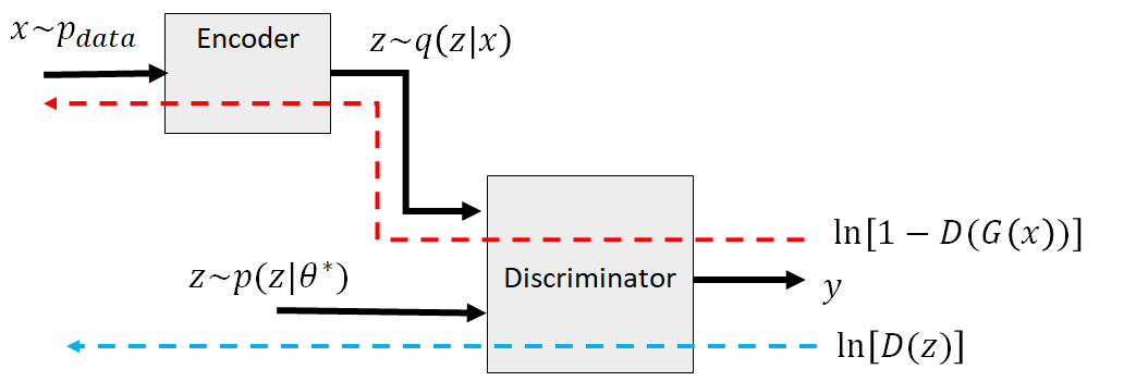
Figure 1: Proposed deep clustering loss using adversarial net. It uses the discriminator and encoder architecture inspired by GAN.

IV-A Training the discriminator

For discussion purpose, we only use a one hidden layer MLP for the encoder and the discriminator. Extending it to two or more hidden layers is straightforward. We use a MLP structure $x_{i}-h_{j}-z_{\varsigma}$ for our encoder and $z_{\varsigma}-h_{f}-y_{d}$ for our discriminator. The hidden layers are defined as $h_{f}$, $h_{j}$ and $z_{\varsigma}$ (encoder output) respectively. We train the discriminator weight $\left\{w_{fd},w_{\varsigma f}\right\}$ by feeding it with $1...N$ positive and negative samples. For the sake of brevity, we refer to each $n^{th}$ sample of $x$ as $x^{\left(n\right)}$ with dimension $I$. In the forward pass in Fig 1, samples go to the discriminator through path B and R. Samples generated from deep clustering space¹ (path B) are positive i.e. $T=1$ and samples generated from latent space (path R) are negative i.e. $T=0$. Cross-entropy loss is defined for $L_{2}$ and $L_{1}$ using the following:

$$\begin{array}[]{c}D=y^{T}(1-y)^{1-T}\\ L_{1}=\ln D(z)\\ L_{2}=\ln\left[1-D(G(x))\right]\end{array}$$ (6)

The activation function for each layer is represented as $\sigma\left(\cdot\right)$. We define the neural network output and target label as $y=\left\{0,1\right\}$ and $T=\left\{0,1\right\}$ respectively. Both $y$ and $T$ have the same dimension $d$.

Neural Network R: We perform weight update using eqn (7) via stochastic gradient ascent (SGA). As we seek sampling from $p(z\mid\theta^{*})$ instead of $q(z\mid x)$, we set $T=0$ for $D$.

$$\begin{array}[]{c}L_{2}=\left\{\frac{1}{N}\sum_{n=1}^{N}\;\underset{x^{\left(n\right)}\sim p_{data}}{E}\left[\ln\left(1-D\left(G(x^{\left(n\right)})\right)\right)\right]\right\}\end{array}$$ (7)

Neural Network B: The deep clustering parameters $\theta=\{\eta,\tau,\zeta\}$ are defined as

$$\begin{array}[]{c}\eta_{k}=\frac{1}{N}\sum_{n=1}^{N}\;z^{(n)}\in k\\ \tau_{k}=\left(\frac{1}{N}\sum_{n=1}^{N}\;\left(z^{(n)}-\eta_{k}\right)^{2}\right)^{-1}\in k\\ \zeta^{(n)}=\arg\max_{k}\left\{\;\ln p(z^{(n)}\mid\eta_{k},\tau_{k})\;\right\}\forall k\end{array}$$ (8)

Since the samples in the latent space displaces each time the encoder weight changes, GMM has to be re-computed each time the weight is updated. After sampling from GMM i.e. $z\sim p(z\mid\theta^{*})$ and setting $T=1$ to $D$, we perform weight update using eqn (9).

$$\begin{array}[]{c}L_{1}=\left\{\frac{1}{N}\sum_{n=1}^{N}\;\underset{z^{\left(n\right)}\sim p(z|\theta^{*})}{E}\left[\ln D\left(z^{\left(n\right)}\right)\right]\right\}\end{array}$$ (9)

IV-B Training the encoder

The encoder $q(z\mid x)$ maps $x$ to $z$ in the latent space. However, we desire to minimize between $q(z\mid x)$ and $p(z\mid\theta^{*}).$ Meaning that we desire to produce a sample $z$ from $q(z\mid x)$ that is as close as possible to the sampling from $p(z\mid\theta^{*})$.

Neural Network R: There is only the discriminator path which updates the encoder weight in Fig 1. Given $N$ samples, eqn (10) computes the SGA weight update for the encoder for $T=0$.

$$\begin{array}[]{c}L_{2}=\left\{\frac{1}{N}\sum_{n=1}^{N}\;\underset{x^{\left(n\right)}\sim p_{data}}{E}\left[\ln\left(1-D\left\{G(x^{\left(n\right)})\right\}\right)\right]\right\}\end{array}$$ (10)

V Experiments

We selected some benchmarked datasets used by deep clustering for our experiments in Tables II-VI. There are several factors affecting deep clustering. i) The clustering algorithm used in the latent space e.g. Kmeans or GMM. ii) The number of hidden layers and nodes of the neural network. iii) The gradient ascent method used for training the loss functions. iv) The activation functions used.

For DCAN, we use $tanh$ for the hidden layers and $sigmoid$ for the output. We set the clustering iteration to one in Table II and a sufficient statistics of at least 600 points in the raw latent space to estimate the cluster parameters. The number of cluster is the same as the number of classes. We use a minibatch size of $N=16$ samples, 500 iterations and we use gradient ascent with momentum with a learning rate between $10^{-3}$ and $10^{-5}$. We use accuracy (ACC) and normalized mutual information (NMI) [15] to evaluate the performance of our clustering.

There is a tradeoff between clustering accuracy and the dimension reduction representation in the latent space for deep clustering. As compared to most non deep clustering objectives which use a bottleneck latent space (e.g. $Z=10$), we found that having a large dimension for the latent state (e.g. $Z=128$) is crucial for clustering. This is because when the dimensionality is not sufficiently large, there will be alot of overlapping clusterings in the latent space. Empirically, we observed that when the dimension of the latent space is too small, the accuracy obtained will be much lower. This effect can vary between 10 to 20% accuracy for most of the datasets we have tried.

SVHN: A real images dataset containing 10 digits class of house numbers but it is a more complex and challenging dataset than MNIST [16]. The images in SVHN are natural and not clean who have much variance in illumination and distraction. We took a 1K samples per class for 10 classes or 10K random samples in total. We are using Resnet18 [17] as the image feature extraction with a dimension of 512. For this experiment, we use an autoencoder with a single hidden layer with a size of 256 neurons for the encoder (and vice-versa for the decoder) and the latent space has 128 neurons. In Table 2, the average ACC of Kmeans in the original feature space is 0.6815. The latent space trained by reconstruction loss showed clustering performance at an average ACC of 0.7373. The latent space of VAE showed better result when performing Kmeans at 0.7663. But it could not achieve the same performance gained by deep clustering approaches. When performing Kmeans in the latent space of ABC, the average ACC is at 0.8872. Lastly, DCAN performed better result than ABC at 0.9047.

USPS: This is a simple 10 digits class dataset that does not have background noise like SVHN. The training size is 7291 and the testing size is 2007. The raw pixel values of each 16x16 image is flattened to 256 and used as inputs to all the comparisons. Our setup uses $256-196-128$ for the encoder and $128-16-1$ for the discriminator. Kmeans or GMM in the latent space of deep clustering methods such as DC-GMM, ABC, DEC and DCAN outperformed other latent spaces such as using reconstruction loss. This is seen when comparing ABC at 0.715 to AE at 0.6081 in Table III. DCAN outperforms all the methods at $0.8276$.

MNIST: A well cited 10 digit classes dataset with no background but it has more samples than USPS. The train and test sample size is at 50K and 10K. Our settings are $196-384-256$ for the encoder and $256-16-1$ for the decoder. The input dimension is originally at $28\times 28$ but we have downsampled it to $14\times 14$ and flattened to 196. We have also experimented using the original image at $28\times 28$ and flattened to 384 for the encoder at $784-512-384-256$ but the accuracy is slightly poorer. In Table IV, DCAN using raw pixel information obtained $0.8565$ for ACC which is on par or better than the unsupervised deep learning methods including DASC, DEC, DCN and DC-GMM. However on MNIST, most deep clustering methods could not obtain the performance of recent deep learning methods such as KINGDRA, DAC and IMSAT as their goals are much more ACC result oriented. For KINGDRA, it combines several ideas together including ladder network [18] and psuedo-label learning [19] for the neural network and using ensemble clustering. In DAC, their approach is based on pairwise classification. In IMSAT-RPT, the neural network was trained by augmenting the training dataset. In this paper however, we are mainly focused on improving the concept of the Euclidean distance based deep learning using ABC. DCAN penalizes samples for being an outlier from their cluster centers and does so uniquely by using the discriminator to penalize the encoder.

The original objective of deep clustering is specifically aimed at clustering. In some datasets, the latent space of this objective do not necessarily co-serve as the most important factor for raw pixel feature extraction. Thus, we used ResNet18 pretrained model as a feature extractor for MNIST, prior to deep clustering. The new ACC for DCAN improved to 0.995 and in fact outperforms KINGDRA as well as all the recent non deep clustering methods.

CIFAR10: A 10 classes object categorization dataset with 50K training and 10K testing of real images. On CIFAR10, most deep clustering methods have difficulty performing end-to-end learning. As compared to deep ConvNet which utilizes convolutional neural network and supervised learning for a specific task (i.e. feature extraction), deep clustering typically rely on fewer hidden layer in the encoder for end-to-end learning (i.e. both feature extraction and deep clustering). Thus, we followed the experiment setup in [20] by using the “avg pool” layer of ResNet50 as a feature extractor with a dimension of 2048. The ResNet50 [17] model is pretrained on ImageNet. In Table V, DCAN uses $2048-1024-512-128$ and $128-16-1$ respectively for the encoder and discriminator. Despite the stronger performance of DAC, IMSAT and KINGDRA on MNIST, we outperformed these comparisons on CIFAR10 at $0.5844$. This is despite the fact that both KINGDRA and IMSAT also use ResNet50 pretrained on ImageNet.

Reuters-10k: The Reuters-10k dataset according to [21, 22] contains 10K samples with 4 classes and the feature dimension is 2000. End-to-end learning is performed on this dataset. We compared DCAN to other unsupervised deep learning approaches. DCAN uses $2000-100-500$ and $500-100-1$ respectively for the encoder and discriminator. In Table VI, we observed that Kmeans alone can achieve an ACC of 0.6018 on the raw feature dimension. Most deep learning methods can achieve between 0.69 to 0.73 on this dataset. DCAN was able to obtain the best ACC at 0.7867.

INITIALIZATION:

 

initialize clusters in latent space using Kmeans

initialize encoder and discriminator weights

 

MAIN:

 

for epoch=1:EPOCH

      

1) draw a minibatch $x=\left\{x_{n}\right\}_{n=1}^{N}\in\mathbb{R^{\mathbf{\mathrm{I}}}}$ which contains data space sample

2) forward pass $x$ through encoder to obtain a matrix, $LATENT\in\mathbb{R^{\mathbf{\mathrm{N\times I}}}}$ in the latent space

      

for iteration=1:ITERATION

3) train Kmeans parameters $\eta,\zeta$ using $LATENT$

end

      

for minibatch=1:MINIBATCH

4) draw a sample $x_{n}$

5) discriminator: compute network weight using $L_{1}$ and $\eta,\tau,\zeta$ for $T=1$

6) discriminator: compute network weight using $L_{2}$ for $T=0$

7) encoder: compute network weight using $L_{1}$ for $T=0$

end

      

      8) update discriminator and encoder weights

 

end

Algorithm 1 Pseudocode of DCAN

VI Conclusion

We proposed DCAN, a non closed form approach to deep clustering over traditional closed form Euclidean or KL divergence loss function. The objective of traditional deep clustering is to optimize the autoencoder latent space with clustering information. The key to this technique lies in a loss function that minimizes both Kmeans partitioning and distribution of the samples in the latent space. Despite the recent success of deep clustering, there are some concerns: i) How to extend the inputs within the loss function to probabilistic models? ii) Can we backpropagate the neural network when there is no closed form learning for the probabilistic function. This paper addresses these two concerns both in theory and a proposed approach for a novel deep clustering approach based on adversarial net.

neural network objective	cluster algo.	method	ACC
-	Kmeans	Kmeans	0.6815
recon. loss	Kmeans	AE	0.7373
recon. + Gaussian prior loss	Kmeans	VAE [10]	0.7663
recon. + clust. loss	Kmeans	ABC [7]	0.8872
		Proposed Method
adversarial net based clust. loss	Kmeans	DCAN (deep features)	0.9047

Table II: SVHN

neural network objective	cluster algo.	method	ACC
-	Kmeans	Kmeans [7]	0.674
-	NCUT	NCUT [7]	0.696
-	Spectral	Spectral [7]	0.693
recon. loss	Kmeans	AE[23]	0.6081
recon. + Euclidean dist. clust. loss	Kmeans	ABC[7]	0.715
KLD clust. loss	Student’s t-dist.	DEC [22]	0.6246
recon. + Euclidean dist. clust. loss	Kmeans	DC-Kmeans [21]	0.6442
recon. + Euclidean dist. clust. loss	GMM	DC-GMM [21]	0.6476
		Proposed Method
adversarial net based clust. loss	Kmeans	DCAN (raw pixels)	0.8276

Table III: USPS

neural network objective	cluster algo.	method	ACC
-	Kmeans	Kmeans [7]	0.535
-	NCUT	NCUT [7]	0.543
-	Spectral	Spectral [7]	0.556
recon. loss	Kmeans	AE [23]	0.6903
recon. + Euclidean dist. clust. loss	Kmeans	ABC [7]	0.760
recon. + Euclidean dist. clust. loss	Kmeans	DC-Kmeans [21]	0.8015
recon. + Euclidean dist. clust. loss	GMM	DC-GMM [21]	0.8555
KLD clust. loss	Student’s t-dist.	DEC [22]	0.843
recon. + Euclidean dist. clust. loss	Kmeans	DCN [14]	0.830
adversarial net based subspace loss	Affinity matrix	DASC [13]	0.804
self-augmented training	RIM	IMSAT-RPT [24]	0.896
pairwise-classification	cosine distance	DAC [25]	0.9775
ladder network	ensemble	KINGDRA-LADDER-1M [20]	0.985
		Proposed Method
adversarial net based clust. loss	Kmeans	DCAN (raw pixels)	0.8565
adversarial net based clust. loss	Kmeans	DCAN (deep features)	0.995

Table IV: MNIST

neural network objective	cluster algo.	method	ACC
KLD clust. loss	Student’s t-dist.	DEC [22]	0.469
self-augmented training	RIM	IMSAT-RPT [24]	0.455
pairwise-classification	cosine distance	DAC [25]	0.5218
ladder network	ensemble	KINGDRA-LADDER-1M [20]	0.546
		Proposed Method
adversarial net based clust. loss	Kmeans	DCAN (deep features)	0.5844

Table V: CIFAR10

neural network objective	clustering	method	ACC
-	Kmeans	Kmeans	0.6018
recon. + Euclidean dist. clust. loss	Kmeans	ABC	0.7019
recon. + Euclidean dist. clust. loss	Kmeans	DC-Kmeans [21]	0.7301
recon. + Euclidean dist. clust. loss	GMM	DC-GMM [21]	0.6906
KLD clust. loss	Student’s t-dist.	DEC [22]	0.7217
self-augmented training	Kmeans	IMSAT-RPT [24]	0.719
ladder network	ensemble	KINGDRA-LADDER-1M [20]	0.705
		Proposed Method
adversarial net based clust. loss	Kmeans	DCAN (raw features)	0.7867

Table VI: Reuters-10k

References

- [1] E. Karamatli, A. T. Cemgil, S. Kirbiz, Audio source separation using variational autoencoders and weak class supervision, IEEE Signal Processing Letters (2019) 1–1doi:10.1109/LSP.2019.2929440.
- [2] P. Last, H. A. Engelbrecht, H. Kamper, Unsupervised feature learning for speech using correspondence and siamese networks, IEEE Signal Processing Letters 27 (2020) 421–425. doi:10.1109/LSP.2020.2973798.
- [3] W. Huang, M. Yin, J. Li, S. Xie, Deep clustering via weighted -subspace network, IEEE Signal Processing Letters 26 (11) (2019) 1628–1632.
- [4] K.-L. Lim, X. Jiang, C. Yi, Deep clustering with variational autoencoder, IEEE Signal Processing Letters 27 (2020) 231–235.
- [5] A. M. Abdelhameed, M. Bayoumi, Semi-supervised eeg signals classification system for epileptic seizure detection, IEEE Signal Processing Letters 26 (12) (2019) 1922–1926.
- [6] M. Han, O. Ozdenizci, Y. Wang, T. Koike-Akino, D. Erdogmus, Disentangled adversarial autoencoder for subject-invariant physiological feature extraction, IEEE Signal Processing Letters 27 (2020) 1565–1569. doi:10.1109/LSP.2020.3020215.
- [7] C. Song, F. Liu, Y. Huang, L. Wang, T. Tan, Auto-encoder based data clustering, in: Iberoamerican Congress on Pattern Recognition, Springer, 2013, pp. 117–124.
- [8] E. Min, X. Guo, Q. Liu, G. Zhang, J. Cui, J. Long, A survey of clustering with deep learning: From the perspective of network architecture, IEEE Access 6 (2018) 39501–39514.
- [9] Z. Jiang, Y. Zheng, H. Tan, B. Tang, H. Zhou, Variational deep embedding: an unsupervised and generative approach to clustering, in: Proceedings of the 26th International Joint Conference on Artificial Intelligence, AAAI Press, 2017, pp. 1965–1972.
- [10] D. P. Kingma, M. Welling, Stochastic gradient vb and the variational auto-encoder, in: Second International Conference on Learning Representations, ICLR, 2014.
- [11] I. Goodfellow, J. Pouget-Abadie, M. Mirza, B. Xu, D. Warde-Farley, S. Ozair, A. Courville, Y. Bengio, Generative adversarial nets, in: Advances in neural information processing systems, 2014, pp. 2672–2680.
- [12] A. Makhzani, J. Shlens, N. Jaitly, I. Goodfellow, Adversarial autoencoders, in: International Conference on Learning Representations, 2016.
- [13] P. Zhou, Y. Hou, J. Feng, Deep adversarial subspace clustering, in: Proceedings of the IEEE Conference on Computer Vision and Pattern Recognition, 2018, pp. 1596–1604.
- [14] B. Yang, X. Fu, N. D. Sidiropoulos, M. Hong, Towards k-means-friendly spaces: Simultaneous deep learning and clustering, in: Proceedings of the 34th International Conference on Machine Learning-Volume 70, JMLR. org, 2017, pp. 3861–3870.
- [15] D. Cai, X. He, J. Han, Document clustering using locality preserving indexing, IEEE Transactions on Knowledge and Data Engineering 17 (12) (2005) 1624–1637.
- [16] Y. LeCun, L. Bottou, Y. Bengio, P. Haffner, Gradient-based learning applied to document recognition, Proceedings of the IEEE 86 (11) (1998) 2278–2324.
- [17] K. He, X. Zhang, S. Ren, J. Sun, Deep residual learning for image recognition, in: Proceedings of the IEEE Conference on Computer Vision and Pattern Recognition, 2016, pp. 770–778.
- [18] A. Rasmus, M. Berglund, M. Honkala, H. Valpola, T. Raiko, Semi-supervised learning with ladder networks, in: Advances in neural information processing systems, 2015, pp. 3546–3554.
- [19] D.-H. Lee, Pseudo-label: The simple and efficient semi-supervised learning method for deep neural networks, in: Workshop on challenges in representation learning, ICML, Vol. 3, 2013.
- [20] D. Gupta, R. Ramjee, N. Kwatra, M. Sivathanu, Unsupervised clustering using pseudo-semi-supervised learning, in: International Conference on Learning Representations, 2020.
- [21] K. Tian, S. Zhou, J. Guan, Deepcluster: A general clustering framework based on deep learning, in: Joint European Conference on Machine Learning and Knowledge Discovery in Databases, Springer, 2017, pp. 809–825.
- [22] J. Xie, R. Girshick, A. Farhadi, Unsupervised deep embedding for clustering analysis, in: International conference on machine learning, 2016, pp. 478–487.
- [23] G. E. Hinton, R. R. Salakhutdinov, Reducing the dimensionality of data with neural networks, science 313 (5786) (2006) 504–507.
- [24] W. Hu, T. Miyato, S. Tokui, E. Matsumoto, M. Sugiyama, Learning discrete representations via information maximizing self-augmented training, in: Proceedings of the 34th International Conference on Machine Learning-Volume 70, JMLR. org, 2017, pp. 1558–1567.
- [25] J. Chang, L. Wang, G. Meng, S. Xiang, C. Pan, Deep adaptive image clustering, in: Proceedings of the IEEE international conference on computer vision, 2017, pp. 5879–5887.