High Quality QCD Axion via Electric-Magnetic Duality

Abstract

We propose a novel paradigm for the QCD axion with high-quality Peccei-Quinn (PQ) symmetry on the basis of electric-magnetic duality in the conformal window of a supersymmetric gauge theory. PQ breaking fields, that contain the QCD axion, emerge in the magnetic theory and possess a large anomalous dimension, which leads to not only generation of an intermediate scale of spontaneous PQ breaking but also significant suppression of explicit PQ symmetry breaking operators. The high PQ quality and the absence of a Landau pole in the color gauge coupling are achieved. The parameter space to realize the correct abundance of the axion dark matter (DM) predicts explicit PQ violation which may be probed by future measurements of the neutron electric dipole moment. In the other viable parameter space, the lightest supersymmetric particle can become a DM candidate. Since the model naturally accommodates a mechanism to suppress the axion isocurvature fluctuation, it provides a complete solution to the strong CP problem as well as the identity of DM.

I Introduction

The strong CP problem is a major unsolved question in the Standard Model (SM) of particle physics. Non-observation of the neutron electric dipole moment (EDM) puts a bound on the strong CP phase, $|\bar{\theta}|\lesssim 10^{-10}$ Baker et al. (2006); Pendlebury et al. (2015). That is, CP violation is unnaturally suppressed in quantum chromodynamics (QCD). The most popular solution to the problem is based on the Peccei-Quinn (PQ) mechanism Peccei and Quinn (1977), where a spontaneously broken global symmetry is introduced, resulting in the associated pseudo-Nambu-Goldstone mode, called the axion Weinberg (1978); Wilczek (1978). Since the vacuum expectation value (VEV) of the axion field is set to a CP conserving vacuum below the QCD scale, the strong CP phase $\bar{\theta}$ is cancelled out dynamically. Interestingly, in the early Universe, the coherent oscillation of the same axion field behaves as a matter fluid and can be a dominant component of dark matter (DM) Preskill et al. (1983); Abbott and Sikivie (1983); Dine and Fischler (1983). The nature of the axion is controlled by the axion decay constant $f_{a}$ which is constrained as $10^{8}\ {\rm GeV}\lesssim f_{a}\lesssim 10^{12}\ {\rm GeV}$, where the lower bound comes from the astrophysical cooling argument Mayle et al. (1988); Raffelt and Seckel (1988); Turner (1988); Chang et al. (2018); Carenza et al. (2019); Leinson (2014); Hamaguchi et al. (2018); Leinson (2019); Buschmann et al. (2022) and the upper bound is put by imposing a condition that the axion DM is not overproduced for a natural initial amplitude of the axion oscillation. Since the axion mass and coupling strength with SM particles depend on $f_{a}$, various searches for the axion are currently ongoing and planned in a vast range of $f_{a}$ (for a summary of the current status, see Ref. O’Hare (2020)).

While the axion is attractive as a solution to the strong CP problem and a DM candidate, there still remain questions to be answered. One is why spontaneous breaking of the PQ symmetry occurs at such an intermediate scale hierarchically smaller than the Planck scale, inducing the instability of $f_{a}$ against radiative corrections from higher scale physics. Another issue is the quality of the global PQ symmetry Dine and Seiberg (1986); Barr and Seckel (1992); Kamionkowski and March-Russell (1992a, b); Holman et al. (1992); Kallosh et al. (1995); Carpenter et al. (2009a, b). In order to solve the strong CP problem, any extra correction to the axion potential must be suppressed at the level of $\mathcal{O}(10^{-10})$, which is incompatible with quantum gravity effects Kallosh et al. (1995); Banks and Seiberg (2011); Witten (2018); Harlow and Ooguri (2019, 2021). A way to solve these two questions is to make the axion composite Kim (1985); Choi and Kim (1985); Randall (1992); Izawa et al. (2002); Yamada et al. (2016); Redi and Sato (2016); Di Luzio et al. (2017); Lillard and Tait (2017, 2018); Gavela et al. (2019); Lee and Yin (2019); Yamada and Yanagida (2021); Ishida et al. (2022); Contino et al. (2022). The scale of $f_{a}$ is dynamically generated by dimensional transmutation in a high-energy gauge theory with quarks that form the composite axion after the confinement, and the theory does not allow dangerous interactions explicitly violating the PQ symmetry so that the axion quality problem is ameliorated. However, one general issue of a composite axion model is that since many new colored particles are introduced to the model, the SM color gauge coupling easily hits a Landau pole. Another approach is the use of (super)conformal dynamics Nakai and Suzuki (2021); Nakagawa et al. (2024). That is, a PQ breaking scalar field couples to a conformal field theory (CFT) and holds a large anomalous dimension, which leads to a significant suppression of PQ-violating higher-dimensional operators expected from quantum gravity effects. A marginally-relevant operator triggers spontaneous breaking of the PQ symmetry at an intermediate scale. The conformal invariance is also spontaneously broken, generating a mass gap in the CFT. Although this model can significantly ameliorate the axion quality problem, its complete solution is only achieved in a limited parameter space with a small gravitino mass.

In the present paper, we explore a new paradigm that a high-quality axion emerges through electric-magnetic duality in an $\mathcal{N}=1$ supersymmetric non-Abelian gauge theory Seiberg (1995): two different (electric and magnetic) gauge theories describe the same long distance physics. What is amazing in this duality is that the weakly interacting region of one theory is mapped to the strongly interacting region of the other. To build a high-quality axion model, we define our electric theory in conformal window at a UV scale. Then, the theory flows into a conformal fixed point where the magnetic theory gives a better description and contains PQ breaking fields. As we will see, the generation of the scale $f_{a}$ and the axion quality problem are addressed by a combination of mechanisms realized in the composite and conformal axion models. Hence, the model occupies an intermediate position between the composite and conformal axions: a larger number of color in the electric theory, which tends to suffer from a Landau pole in the ordinary QCD gauge coupling, would lead to the composite axion, while a smaller number of color would make the electric theory a better description, realizing the conformal axion (in this case, we need to introduce elementary PQ breaking fields). Then, the problems in the composite and conformal axion models are potentially resolved. In fact, we will see that the high PQ quality and the absence of a Landau pole in the color gauge coupling are achieved at the same time. Furthermore, it will be shown that the model possesses an intrinsic mechanism to suppress the isocurvature fluctuation of the light axion and significantly relax a constraint on the scale of inflation.

The rest of the paper is organized as follows. In Sec. II, we present our axion model in both electric and magnetic pictures, and discuss the generation of the PQ symmetry breaking scale. The stabilization of the saxion direction with supersymmetry (SUSY) breaking is also performed. Sec. III studies the issue of a Landau pole in the QCD gauge coupling. In Sec. IV, we estimate the quality of the PQ symmetry and identify a viable parameter space of the model. Sec. V discusses implications on the DM in our model and the issue of isocurvature fluctuations. Finally, Sec. VI is devoted to conclusions and discussions.

	$Q_{a}$	$\bar{Q}^{a}$	$Q_{\alpha}$	$\bar{Q}^{\alpha}$	$\eta_{a}^{~b}$	$\xi_{\alpha}^{~\beta}$	$Z_{a}^{~\alpha}$	$\bar{Z}_{\alpha}^{~a}$
$SU(N)$	$\square$	$\bar{\square}$	$\square$	$\bar{\square}$	${\bm{1}}$	${\bm{1}}$	${\bm{1}}$	${\bm{1}}$
$SU(N_{F}/2)_{1}$	$\square$	$\bar{\square}$	${\bm{1}}$	${\bm{1}}$	Adj	${\bm{1}}$	$\square$	$\bar{\square}$
$SU(N_{F}/2)_{2}$	${\bm{1}}$	${\bm{1}}$	$\square$	$\bar{\square}$	$\bm{1}$	Adj	$\bar{\square}$	$\square$
$U(1)_{\rm PQ}(\supset Z_{\widetilde{N}})$	$\chi_{1}$	$\chi_{2}$	$-\chi_{2}$	$-\chi_{1}$	$-1$	$1$	$0$	$0$
$U(1)_{R}$	$\frac{N_{F}-N}{N_{F}}$	$\frac{N_{F}-N}{N_{F}}$	$\frac{N_{F}-N}{N_{F}}$	$\frac{N_{F}-N}{N_{F}}$	$\frac{2N}{N_{F}}$	$\frac{2N}{N_{F}}$	$\frac{2N}{N_{F}}$	$\frac{2N}{N_{F}}$

Table 1: The charge assignments in the electric theory.

II The Model

We define our axion model with its electric picture and then discuss the magnetic dual. The generation of the PQ symmetry breaking scale is described by using the magnetic theory. The axion couplings to gluons and photons are also presented. Finally, we introduce SUSY breaking and perform the saxion stabilization.

II.1 Electric theory

Let us consider a supersymmetric $SU(N)$ gauge theory with $N_{F}$ pairs of vectorlike quarks, $Q$ and $\bar{Q}$, which belong to the (anti-)fundamental representation of $SU(N)$. The theory is in conformal window and flows into a nontrivial IR fixed point Intriligator and Seiberg (2007). Here, our focus is on the case that the number of flavors is an even number, parameterized as $N_{F}=2N-\delta$ with $\delta=2,4,6,\dots(<N/2)$. We then divide the quarks $Q,\bar{Q}$ into two parts, represented by $Q_{a}(\bar{Q}^{a}),Q_{\alpha}(\bar{Q}^{\alpha})$ with $a\in(1,\dots,N_{F}/2)$ and $\alpha$ $\in(N_{F}/2+1,\dots,N_{F})$, and assign them with different charges under the global $U(1)_{\rm PQ}$ symmetry. In addition, we introduce gauge-singlet chiral supermultiplets, $\eta_{a}^{~b},\xi_{\alpha}^{~\beta},Z_{a}^{~\alpha},\bar{Z}_{\alpha}^{~a},$ to stabilize extra fields appearing in the magnetic picture, which we will see later. The theory respects $U(1)_{\rm PQ}\times SU(N_{F}/2)_{1}\times SU(N_{F}/2)_{2}$ flavor symmetry. The charge assignments are summarized in Table 1 where we define PQ charges,

$$\chi_{1}\equiv\frac{2N-N_{F}}{2N}\,,\qquad\chi_{2}\equiv\frac{N_{F}}{2N}\,,$$ (1)

so that the $U(1)_{\rm PQ}$ is not anomalous under $SU(N)$ to avoid the axion coupling to the $SU(N)$ gauge field. The assignment of the $U(1)_{R}$ charge is determined by the superconformal nature. The flavor symmetry $SU(N_{F}/2)_{1}$ is weakly gauged and the SM color gauge group $SU(3)_{c}$ as well as the hypercharge $U(1)_{Y}$ is embedded in it. The $U(1)_{\rm PQ}$ symmetry has anomaly under the $SU(3)_{c}$ whose anomaly coefficient is given by $A_{U(1)_{\rm PQ}-SU(3)_{c}-SU(3)_{c}}=-\widetilde{N}$ with $\widetilde{N}\equiv N_{F}-N$. Note that an anomaly-free (or gaugeable) discrete symmetry $Z_{\widetilde{N}}$ remains as a residual symmetry. We impose the discrete symmetry to forbid some explicit $U(1)_{\rm PQ}$ violating operators and realize the PQ symmetry at the renormalizable level.

The symmetry allows the following superpotential with a Planck-suppressed operator:

$$W_{\rm el} = \nu_{1}\eta_{a}^{~b}\bar{Q}^{a}Q_{b}+\nu_{2}\xi_{\alpha}^{~\beta}\bar{Q}^{\alpha}Q_{\beta}$$ (2)

$$+ Z_{b}^{~\alpha}\bar{Q}^{b}Q_{\alpha}+\bar{Z}_{\alpha}^{~b}\bar{Q}^{\alpha}Q_{b}+MZ_{a}^{~\alpha}\bar{Z}_{\alpha}^{~a}$$

$$- \frac{\iota}{M_{\rm Pl}}(\bar{Q}^{a}Q_{a})(\bar{Q}^{\alpha}Q_{\alpha})\,,$$

where $\nu_{1},\nu_{2},\iota$ are dimensionless coupling constants, $M$ is a mass parameter and $M_{\rm Pl}\equiv 1/\sqrt{8\pi G}$ denotes the reduced Planck mass scale with $G$ the Newton constant. We have omitted to explicitly write coupling constants in front of the first and second terms in the second line. As we will see, the Planck-suppressed operator plays an essential role for spontaneous breaking of the $U(1)_{\rm PQ}$ symmetry. At the scale of $M$, the fields $Z,\bar{Z}$ are integrated out, and we obtain the low-energy effective superpotential,

$$W_{\rm el}^{(\rm eff)} = \nu_{1}\eta_{a}^{~b}\bar{Q}^{a}Q_{b}+\nu_{2}\xi_{\alpha}^{~\beta}\bar{Q}^{\alpha}Q_{\beta}$$

$$- \frac{\kappa}{M}(\bar{Q}^{\alpha}Q_{a})(\bar{Q}^{a}Q_{\alpha})-\frac{\iota}{M_{\rm Pl}}(\bar{Q}^{a}Q_{a})(\bar{Q}^{\alpha}Q_{\alpha})\,,$$

where $\kappa$ is introduced as a dimensionless coupling constant.

	$q^{a}$	$\bar{q}_{a}$	$q^{\alpha}$	$\bar{q}_{\alpha}$	$\Phi+\Psi$	$\bar{\Phi}+\bar{\Psi}$	$\Sigma$	$\Xi$	$\eta_{a}^{~b}$	$\xi_{\alpha}^{~\beta}$
$SU(N_{F}-N)$	$\square$	$\bar{\square}$	$\square$	$\bar{\square}$	${\bm{1}}$	${\bm{1}}$	${\bm{1}}$	${\bm{1}}$	${\bm{1}}$	${\bm{1}}$
$SU(N_{F}/2)_{1}$	$\bar{\square}$	$\square$	${\bm{1}}$	${\bm{1}}$	${\bm{1}}$+Adj	${\bm{1}}$	$\square$	$\bar{\square}$	Adj	${\bm{1}}$
$SU(N_{F}/2)_{2}$	${\bm{1}}$	${\bm{1}}$	$\bar{\square}$	$\square$	${\bm{1}}$	${\bm{1}}$+Adj	$\bar{\square}$	$\square$	$\bm{1}$	Adj
$U(1)_{\rm PQ}$	$-1$	$0$	$0$	$1$	$1$	$-1$	$0$	0	$-1$	$1$
$U(1)_{R}$	$\frac{N}{N_{F}}$	$\frac{N}{N_{F}}$	$\frac{N}{N_{F}}$	$\frac{N}{N_{F}}$	$\frac{2(N_{F}-N)}{N_{F}}$	$\frac{2(N_{F}-N)}{N_{F}}$	$\frac{2(N_{F}-N)}{N_{F}}$	$\frac{2(N_{F}-N)}{N_{F}}$	$\frac{2N}{N_{F}}$	$\frac{2N}{N_{F}}$

Table 2: The charge assignments in the magnetic theory.

II.2 Magnetic theory

Corresponding to the presented electric $SU(N)$ gauge theory with $N_{F}\geq N+2$ flavors, there exists the dual magnetic $SU(\widetilde{N})$ gauge theory Seiberg (1995), which contains $N_{F}$ vectorlike pairs of dual quarks $q,\bar{q}$ and $N_{F}^{2}$ gauge singlets $\mathcal{M}_{i}^{~j}$ with $i,j=1,2,\cdots N_{F}$, as well as $\eta_{a}^{~b},\xi_{\alpha}^{~\beta}$ introduced in the electric theory. The superpotential includes $W_{\rm mag}\supset q\mathcal{M}\bar{q}$. Note that the magnetic dual theory is also in conformal window. According to the flavor structure of our model, the gauge singlets $\mathcal{M}$ can be decomposed in terms of $N_{F}/2\times N_{F}/2$ matrices:

$$\mathcal{M}\equiv\left(\begin{array}[]{cc}\Phi\delta_{a}^{b}+\Psi_{a}^{~b}&\Sigma_{a}^{~\beta}\\ \Xi_{\alpha}^{~b}&\bar{\Phi}\delta_{\alpha}^{\beta}+\bar{\Psi}_{\alpha}^{~\beta}\\ \end{array}\right).$$ (6)

Here, $\Phi\,(\bar{\Phi})$ and $\Psi\,(\bar{\Psi})$ are defined as the trace and traceless parts of $\mathcal{M}_{a}^{~b}\,(\mathcal{M}_{\alpha}^{~\beta})$, respectively. Table 2 summarizes the charge assignments in the magnetic dual theory. We note that the ‘t Hooft anomaly ’t Hooft (1980) is matched between the electric and magnetic theories. In particular, the $U(1)_{\rm PQ}$ symmetry has anomaly under $SU(3)_{c}$ with the same anomaly coefficient as the electric theory, $A_{U(1)_{\rm PQ}-SU(3)_{c}-SU(3)_{c}}=-\widetilde{N}$.

The correspondence between the gauge singlets $\mathcal{M}$ in the magnetic theory and the quark bilinears in the electric theory is written as

$$(\Phi+\Psi)_{a}^{~~b}\leftrightarrow\frac{\bar{Q}^{b}Q_{a}}{\Lambda^{\prime}}\,, (\bar{\Phi}+\bar{\Psi})_{\alpha}^{~~\beta}\leftrightarrow\frac{\bar{Q}^{\beta}Q_{\alpha}}{\Lambda^{\prime}}\,,$$

$$\Sigma_{a}^{~~\beta}\leftrightarrow\frac{\bar{Q}^{\beta}Q_{a}}{\Lambda^{\prime}}\,, \Xi_{\alpha}^{~~b}\leftrightarrow\frac{\bar{Q}^{b}Q_{\alpha}}{\Lambda^{\prime}}\,.$$ (7)

Here, the normalization factor $\Lambda^{\prime}$ is a holomorphic and charge neutral scale and given in terms of the holomorphic scale in the electric theory $\Lambda_{\rm el}$ and that in the magnetic theory $\Lambda_{\rm mag}$:

$$\Lambda^{\prime N_{F}}=(-1)^{N-N_{F}}\Lambda_{\rm el}^{3N-N_{F}}\Lambda_{\rm mag}^{3(N_{F}-N)-N_{F}}\,.$$ (8)

In the following discussion, we assume $\Lambda^{\prime}\simeq\Lambda_{\rm el}\simeq\Lambda_{\rm mag}$. Then, corresponding to the superpotential of the electric theory in Eq. (LABEL:Weleff), the superpotential of the magnetic theory is given by

$$W_{\rm mag} = \lambda(\Phi q^{a}\bar{q}_{a}+q^{a}\Psi_{a}^{~b}\bar{q}_{b})+\bar{\lambda}(\bar{\Phi}q^{\alpha}\bar{q}_{\alpha}+q^{\alpha}\bar{\Psi}_{\alpha}^{~\beta}\bar{q}_{\beta})$$ (9)

$$+ \rho q^{a}\Sigma_{a}^{~\beta}\bar{q}_{\beta}+\bar{\rho}q^{\alpha}\Xi_{\alpha}^{~b}\bar{q}_{b}-M_{\Phi}\Phi\bar{\Phi}-M_{\Sigma\Xi}\Sigma_{a}^{~\alpha}\Xi_{\alpha}^{~a}$$

$$+ \nu_{1}\Lambda^{\prime}\eta_{a}^{~b}\Psi_{b}^{~a}+\nu_{2}\Lambda^{\prime}\xi_{\alpha}^{~\beta}\bar{\Psi}_{\beta}^{~\alpha}\,,$$

where $\lambda,\bar{\lambda},\rho,\bar{\rho}$ denote constant coefficients, and we have introduced new dimensionful parameters,

$$M_{\Phi}\equiv\iota\left(\frac{N_{F}}{2}\right)^{2}\frac{\Lambda^{\prime 2}}{M_{\rm Pl}}\,,\qquad M_{\Sigma\Xi}\equiv\kappa\frac{\Lambda^{\prime 2}}{M}\,.$$ (10)

We can see from Eq. (9) that the fields $\Sigma,\Xi$ form a mass term, and $\Psi,\bar{\Psi}$ form mass terms with $\eta,\xi$, respectively. After integrating out those massive fields, the effective superpotential is given by

$$W_{\rm mag}^{\rm(eff)} = \lambda\Phi q^{a}\bar{q}_{a}+\bar{\lambda}\bar{\Phi}q^{\alpha}\bar{q}_{\alpha}-M_{\Phi}\Phi\bar{\Phi}\,.$$ (11)

When $\Phi,\bar{\Phi}$ develop nonzero VEVs as we will see below, the $U(1)_{\rm PQ}$ symmetry is spontaneously broken, and the $\Phi$ interaction with $q^{a},\bar{q}_{a}$ induces the Chern-Simons term with the $SU(3)_{c}$ gluon in the low-energy effective theory. Thus, our model works as a KSVZ-like QCD axion model Kim (1979); Shifman et al. (1980), with the domain wall number $\widetilde{N}\equiv N_{F}-N$.

II.3 Peccei-Quinn scale

Based on the magnetic description of our model, let us now discuss spontaneous breaking of the $U(1)_{\rm PQ}$ symmetry. In addition to Eq. (11), a non-perturbative effect of supersymmetric QCD (SQCD) generates a superpotential for $\Phi,\bar{\Phi}$ Nakagawa et al. (2024). Assuming $\Phi,\bar{\Phi}$ obtain nonzero VEVs, one can see that the dual quarks $q^{a},\bar{q}_{a}$ and $q^{\alpha},\bar{q}_{\alpha}$ acquire masses of $\lambda\Phi$ and $\bar{\lambda}\bar{\Phi}$, respectively. Then, at the energy scale of those quark masses, they are decoupled. The low-energy effective theory is given by a pure super Yang-Mills which leads to gaugino condensation,

$$W_{\rm gaugino}=(N_{F}-N)\Lambda_{\rm new}^{3}\,,$$ (12)

with

$$\Lambda_{\rm new}^{3}=(\lambda\Phi)^{\frac{N_{F}}{2(N_{F}-N)}}(\bar{\lambda}\bar{\Phi})^{\frac{N_{F}}{2(N_{F}-N)}}\Lambda_{\rm mag}^{\frac{2N_{F}-3N}{N_{F}-N}},$$ (13)

determined by matching the dynamical scales before and after integrating out $q,\bar{q}$. The dynamically generated superpotential (12) and the third mass term in Eq. (11) lead to the $\mathcal{F}$-term potential for the scalar components of $\Phi$ and $\bar{\Phi}$,

$$V_{\mathcal{F}}(\Phi,\bar{\Phi})\cdot Z_{\Phi}$$

$$= \left|M_{\Phi}\Phi-\frac{N_{F}}{2}\bar{\lambda}\Lambda_{\rm mag}^{\frac{2N_{F}-3N}{N_{F}-N}}\left(\lambda\Phi\right)^{\frac{N_{F}}{2(N_{F}-N)}}\left(\bar{\lambda}\bar{\Phi}\right)^{\frac{2N-N_{F}}{2(N_{F}-N)}}\right|^{2}$$

$$+ \left|M_{\Phi}\bar{\Phi}-\frac{N_{F}}{2}\lambda\Lambda_{\rm mag}^{\frac{2N_{F}-3N}{N_{F}-N}}\left(\lambda\Phi\right)^{\frac{2N-N_{F}}{2(N_{F}-N)}}\left(\bar{\lambda}\bar{\Phi}\right)^{\frac{N_{F}}{2(N_{F}-N)}}\right|^{2}.$$

Here, $Z_{\Phi}$ denotes the wavefunction renormalization factor for $\Phi,\bar{\Phi}$. The $\mathcal{F}$-term potential has two degenerate minima:

$$\left\langle\Phi\right\rangle = \left\langle\bar{\Phi}\right\rangle=0\,,$$ (15)

and

$$\left\langle\Phi\bar{\Phi}\right\rangle = \frac{\Lambda_{\rm mag}^{2}}{\lambda\bar{\lambda}}\left(\frac{2M_{\Phi}}{N_{F}\lambda\bar{\lambda}\Lambda_{\rm mag}}\right)^{\frac{2(N_{F}-N)}{2N-N_{F}}}.$$ (16)

While the former vacuum indicates the symmetric phase, the latter vacuum spontaneously breaks the $U(1)_{\rm PQ}$ symmetry. We assume the latter vacuum is realized throughout the history of the Universe.

During the regime where the theory is at the conformal fixed point, the kinetic terms of $\Phi,\bar{\Phi}$ experience a significant wavefunction renormalization due to a large anomalous dimension, which one needs to take into account to find the $U(1)_{\rm PQ}$ breaking scale Nakai and Suzuki (2021). The wavefunction renormalization factors for $\Phi,\bar{\Phi}$ and $q,\bar{q}$ are respectively given by

$$Z_{\Phi} = \left(\frac{M_{c}}{\Lambda}\right)^{-\gamma_{\Phi}},$$ (17)

$$Z_{q} = \left(\frac{M_{c}}{\Lambda}\right)^{-\gamma_{q}},$$ (18)

with $\gamma_{\Phi}\equiv 4-6N/N_{F}$ and $\gamma_{q}\equiv-(2N_{F}-3N)/N_{F}$. Here, $\Lambda$ stands for the scale at which the theory enters into the conformal regime while $M_{c}$ represents the energy scale at which the theory exits from that regime. The canonically normalized $U(1)_{\rm PQ}$ breaking fields $\hat{\Phi},\hat{\bar{\Phi}}$ and dual quarks $\hat{q},\hat{\bar{q}}$ are written as

$$\hat{\Phi}=\sqrt{Z_{\Phi}}\,\Phi\,, ~~\hat{\bar{\Phi}}=\sqrt{Z_{\Phi}}\,\bar{\Phi}\,,$$ (19)

$$\hat{q}^{a(\alpha)}=\sqrt{Z_{q}}\,q^{a(\alpha)}\,, ~~\hat{\bar{q}}_{a(\alpha)}=\sqrt{Z_{q}}\,\bar{q}_{a(\alpha)}\,.$$ (20)

The theory exits from the conformal regime at the scale $M_{c}\sim\lambda\langle|\hat{\Phi}|\rangle\sim\bar{\lambda}\langle|\hat{\bar{\Phi}}|\rangle$. Then, the $U(1)_{\rm PQ}$ breaking scale is given by

$$f_{\rm PQ} \equiv \sqrt{\langle\hat{\Phi}\hat{\bar{\Phi}}\rangle}\simeq\frac{M_{c}}{\sqrt{\lambda\bar{\lambda}}}$$

$$= \left(\frac{\Lambda}{\Lambda_{\rm mag}}\right)^{\frac{N_{F}(2N_{F}-3N)}{3(2N-N_{F})(N_{F}-N)}}\frac{\Lambda}{\sqrt{\lambda\bar{\lambda}}}\left(\frac{2M_{\Phi}}{N_{F}\lambda\bar{\lambda}\Lambda}\right)^{\frac{N_{F}}{3(2N-N_{F})}}$$

$$\simeq \left(\frac{\Lambda_{\rm mag}}{\Lambda}\right)^{\frac{NN_{F}}{3(N_{F}-N)(2N-N_{F})}}\frac{\Lambda}{\sqrt{\lambda\bar{\lambda}}}\left(\frac{\iota N_{F}\Lambda}{2\lambda\bar{\lambda}M_{\rm Pl}}\right)^{\frac{2N-\delta}{3\delta}}.$$

The third equality utilizes Eq. (10) with $\Lambda^{\prime}\simeq\Lambda_{\rm mag}$. While the conformal entering scale $\Lambda$ is determined by solving the renormalization group (RG) equations for the $SU(\widetilde{N})$ gauge coupling $g$ and $\lambda,\bar{\lambda}$ with initial conditions at a UV scale, $\Lambda_{\rm mag}$ is defined as the holomorphic dynamical scale in the magnetic picture. These scales are closely related to each other, depending on the initial condition of the gauge coupling at a UV scale for RG equations. Without any fine tuning, we find $\Lambda/\Lambda_{\rm mag}=\mathcal{O}(1-10^{2})$. One can see from Eq. (LABEL:PQscale) that an intermediate scale of the $U(1)_{\rm PQ}$ breaking $f_{\rm PQ}$ is generated as the scale $\Lambda$ is naturally smaller than the Planck scale. Fig. 1 summarizes hierarchies of scales in our model. We take $M\simeq\Lambda$, so that extra singlet fields decouple at the conformal entering scale $\Lambda$. In the following discussion, we focus on this case for simplicity.

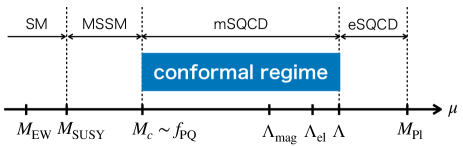
Figure 1: Hierarchies of scales in the model. Here, $M_{\rm SUSY}$ and $M_{\rm EW}$ represent the SUSY and electroweak symmetry breaking scales, respectively. eSQCD and mSQCD denote the electric and magnetic pictures of our model.

We expand the scalar components of the PQ breaking fields around their VEVs, $v\equiv|\langle\hat{\Phi}\rangle|$ and $\bar{v}\equiv|\langle\hat{\bar{\Phi}}\rangle|$:

$$\hat{\Phi}=v\exp\left(\frac{\sigma+ia}{F_{a}}\right),\quad\hat{\bar{\Phi}}=\bar{v}\exp\left(-\frac{\sigma+ia}{F_{a}}\right).$$ (22)

Here, $\sigma,a$ represent the saxion and axion fields, respectively, and $F_{a}/\sqrt{2}\equiv\sqrt{v^{2}+\bar{v}^{2}}$. After integrating out the heavy quark superfields $q,\bar{q}$, the effective theory has the axion-gluon coupling as well as the axion-photon coupling due to anomaly,

$$\mathcal{L}_{a}=\frac{\widetilde{N}}{2}\frac{g_{s}^{2}}{16\pi^{2}}\frac{a}{F_{a}}G_{\mu\nu}^{i}\widetilde{G}^{i\mu\nu}+E\frac{e^{2}}{16\pi^{2}}\frac{a}{F_{a}}F_{\mu\nu}\widetilde{F}^{\mu\nu}\,,$$ (23)

where $g_{s},e$ are the gauge couplings for the $SU(3)_{c}$ and $U(1)_{\rm EM}$, respectively, and $G,\widetilde{G}$ ($F,\widetilde{F}$) denote the gluon (photon) field strength and its dual. The electromagnetic anomaly factor is given by $E=-n_{f}\widetilde{N}q_{\rm EM}^{2}$ where $q_{\rm EM}$ is the $U(1)_{\rm EM}$ charge of $q^{a}$ and $n_{f}$ denotes the number of $q^{a}$ with nonzero $U(1)_{\rm EM}$ charge. Then, the axion decay constant can be defined as $F_{a}/\widetilde{N}$ with the domain wall number identified with $\widetilde{N}$. Taking the basis without the gluon operator, we obtain the usual form of the axion-photon coupling, given by

$$\mathcal{L}_{a\gamma}=\frac{g_{a\gamma}}{4}aF_{\mu\nu}\widetilde{F}^{\mu\nu}\,,$$ (24)

with

$$g_{a\gamma}=\frac{\alpha}{2\pi F_{a}/\widetilde{N}}\left(-2n_{f}q_{\rm EM}^{2}-2.03\right).$$ (25)

Here, $\alpha$ is the fine structure constant, and we have used $m_{u}/m_{d}=0.462$ Workman et al. (2022). Since the sign of the first term in the parenthesis can be changed by the definition of the PQ charge, the axion coupling to photons can be enhanced or suppressed, depending on the $U(1)_{Y}$ charge assignment.

By using Eq. (LABEL:PQscale), the axion decay constant $F_{a}/\widetilde{N}$ is shown in Fig. 2 (orange lines) as a function of the conformal entering scale $\Lambda$. Here we take $N_{F}=2N-2$, $\iota=1$, and $\Lambda/\Lambda_{\rm mag}=5,100$ in the left and right panels, respectively. The values of $\lambda,\bar{\lambda}$ for each $\widetilde{N}$ are determined at the IR fixed point and estimated at the two-loop level by using SARAH Staub (2008) where QCD effects are ignored. The figure demonstrates that an intermediate scale for $F_{a}/\widetilde{N}$ emerges in the theory with much higher scales.

II.4 SUSY breaking

There exists a flat direction in Eq. (16), which we call the saxion. In the SUSY limit, the saxion is massless, but SUSY breaking can deform the flat direction and induce a nonzero saxion mass. Let us consider the following soft SUSY breaking terms for $\hat{\Phi}$, $\hat{\bar{\Phi}}$ and $\hat{q},\hat{\bar{q}}$ in the magnetic theory:

$$\mathcal{L}_{\rm soft}= - \hat{\tilde{q}}^{a*}m^{2}_{q^{a}}\hat{\tilde{q}}^{a}-\hat{\tilde{\bar{q}}}_{a}m^{2}_{\bar{q}_{a}}\hat{\tilde{\bar{q}}}^{*}_{a}$$ (26)

$$- \hat{\tilde{q}}^{\alpha*}m^{2}_{q^{\alpha}}\hat{\tilde{q}}^{\alpha}-\hat{\tilde{\bar{q}}}_{\alpha}m^{2}_{\bar{q}_{\alpha}}\hat{\tilde{\bar{q}}}^{*}_{\alpha}$$

$$- m^{2}_{\Phi}|\hat{\Phi}|^{2}-m^{2}_{\bar{\Phi}}|\hat{\bar{\Phi}}|^{2},$$

where $q,\bar{q}$ with tilde represent their scalar components, and we have ignored SUSY breaking $A$-terms corresponding to the superpotential (11) for simplicity. All soft mass parameters are assumed at around the TeV scale, which is much smaller than the $U(1)_{\rm PQ}$ breaking scale. Taking $m_{q^{a}}^{2}=m_{\bar{q}_{a}}^{2}=m_{q^{\alpha}}^{2}=m_{\bar{q}_{\alpha}}^{2}\equiv\Delta m^{2}$ and using Eq. (11), we obtain the one-loop Coleman-Weinberg potential Coleman and Weinberg (1973),

$$V_{\rm CW}(\hat{\Phi},\hat{\bar{\Phi}})$$

$$=\frac{\widetilde{N}N_{F}}{64\pi^{2}}\Biggl{[}\left(\lambda^{2}|\hat{\Phi}|^{2}+\Delta m^{2}\right)^{2}\log\left(1+\frac{\Delta m^{2}}{\lambda^{2}|\hat{\Phi}|^{2}}\right)$$

$$\quad+\left(\bar{\lambda}^{2}|\hat{\bar{\Phi}}|^{2}+\Delta m^{2}\right)^{2}\log\left(1+\frac{\Delta m^{2}}{\bar{\lambda}^{2}|\hat{\bar{\Phi}}|^{2}}\right)\Biggr{]}\,.$$ (27)

Summing up all contributions, the total scalar potential for $\Phi,\bar{\Phi}$ is expressed as

$$V(\hat{\Phi},\hat{\bar{\Phi}})=V_{\mathcal{F}}+V_{\rm soft}+V_{\rm CW}\,,$$ (28)

where Eq. (LABEL:VF) gives the first term of the right hand side and the soft mass-squared terms give the second contribution.

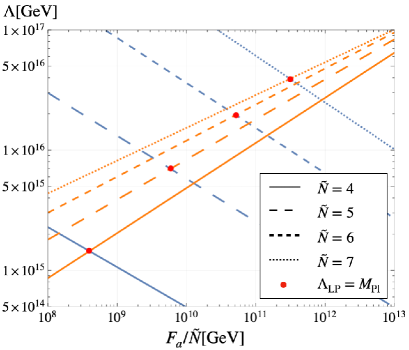
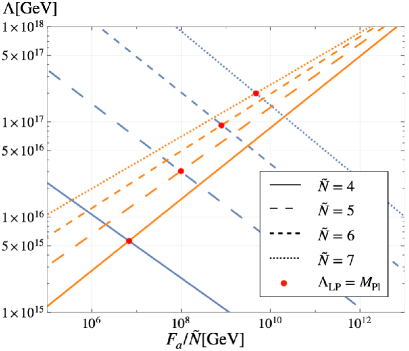
Figure 2: The relation between the conformal entering scale $\Lambda$ and the axion decay constant $F_{a}/\widetilde{N}$ (orange lines). The blue line corresponds to the lower bound to solve the Landau pole problem where $\Lambda$ and $F_{a}/\widetilde{N}$ are assumed to be independent. The allowed region is above each blue line. The intersection of the orange and blue lines, represented by the red dot, is the actual lower bound on $\Lambda$ for each $N$. Here, we take $N_{F}=2N-2,\iota=1,\Lambda/\Lambda_{\rm mag}=5\,(100)$ in the left (right) panel, and use the values of $\lambda,\bar{\lambda}$ estimated at the fixed point.

Since the $F$-term potential $V_{\mathcal{F}}$ is dominant, we can take $\hat{\Phi}\hat{\bar{\Phi}}=f_{\rm PQ}^{2}$ and focus on the flat direction. The VEVs for $\hat{\Phi},\hat{\bar{\Phi}}$ with SUSY breaking effects are then obtained as

$$v \equiv \langle|\hat{\Phi}|\rangle$$ (29)

$$\simeq f_{\rm PQ}\left(\frac{(3\widetilde{N}N_{F}\lambda^{2}/64\pi^{2})\Delta m^{2}+N_{F}m_{\Phi}^{2}/2}{(3\widetilde{N}N_{F}\bar{\lambda}^{2}/64\pi^{2})\Delta m^{2}+N_{F}m_{\bar{\Phi}}^{2}/2}\right)^{1/4}\!\!\!,~~~$$

$$\bar{v} \equiv \langle|\hat{\bar{\Phi}}|\rangle$$ (30)

$$\simeq f_{\rm PQ}\left(\frac{(3\widetilde{N}N_{F}\bar{\lambda}^{2}/64\pi^{2})\Delta m^{2}+N_{F}m_{\bar{\Phi}}^{2}/2}{(3\widetilde{N}N_{F}\lambda^{2}/64\pi^{2})\Delta m^{2}+N_{F}m_{\Phi}^{2}/2}\right)^{1/4}\!\!\!.~~~$$

For $m_{\Phi}^{2}=m_{\bar{\Phi}}^{2}$ and $\lambda=\bar{\lambda}$ which lead to $v=\bar{v}=f_{\rm PQ}$ and the approximation $\Delta m^{2}\ll f_{\rm PQ}^{2}$, we can simply write the saxion mass-squared as

$$m_{\sigma}^{2}\simeq 2m_{\Phi}^{2}+\frac{\widetilde{N}N_{F}\lambda^{2}}{32\pi^{2}}\Delta m^{2}\,.$$ (31)

Note that the saxion direction is stabilized only when the following condition is satisfied:

$$m_{\Phi}^{2}+\frac{\widetilde{N}N_{F}\lambda^{2}}{64\pi^{2}}\Delta m^{2}>0\,.$$ (32)

This condition puts a constraint on the soft SUSY breaking parameters at the $U(1)_{\rm PQ}$ breaking scale $f_{\rm PQ}$. These parameters evolve down to the scale $f_{\rm PQ}$ by RG equations, and hence the proper initial values at a UV scale are required to satisfy the condition. For the RG evolution, see Fig. 2 in Ref. Nakagawa et al. (2024), which we have confirmed that is the same behavior with our case by replacing $N$ by $\widetilde{N}$.

III Landau pole problem

We now investigate the issue of a Landau pole for the SM $SU(3)_{c}$ gauge coupling $g_{s}$ in our model. The one-loop beta function coefficient is given by

$$\beta_{g_{s}} \equiv\mu\frac{\mathrm{d}g_{s}}{\mathrm{d}\mu}$$

$$=-\frac{g_{s}^{3}}{16\pi^{2}}\times\begin{cases}b_{\rm SM}\,,&M_{\rm EW}<\mu<M_{\rm SUSY}\,,\\[4.30554pt] b_{\rm MSSM}\,,&M_{\rm SUSY}<\mu<f_{\rm PQ}\,,\\[4.30554pt] b_{\rm mSQCD}\,,&f_{\rm PQ}<\mu<\Lambda\,,\\[4.30554pt] b_{\rm eSQCD}\,,&\Lambda<\mu<M_{\rm Pl}\,,\end{cases}$$ (33)

where $b_{i}~(i=\rm SM,\,MSSM,\,mSQCD,\,eSQCD)$ are calculated in different effective theories: the SM, MSSM, magnetic picture and electric picture of our model, respectively. The first two coefficients are given by $b_{\rm SM}=7$ and $b_{\rm MSSM}=3$ as usual. Since the $SU(3)_{c}$ is embedded in the weakly gauged $SU(N_{F}/2)_{1}$, the fields charged under $SU(N_{F}/2)_{1}$ in Tab. 1,2 contribute to $b_{\rm mSQCD}$ and $b_{\rm eSQCD}$. For the energy region of $f_{\rm PQ}<\mu<\Lambda$ where the magnetic picture gives a better description, the fields $\eta,\xi,\Psi,\bar{\Psi},\Sigma,\Xi$, which have been integrated out, as well as the $SU(N_{F}/2)_{1}$ singlets $\Phi,\bar{\Phi},q^{\alpha},\bar{q}_{\alpha}$ do not contribute to $b_{\rm mSQCD}$. The first half of magnetic quarks $q^{a},\bar{q}_{a}$, which are $\widetilde{N}=N_{F}-N$ fundamental and anti-fundamental representations of $SU(3)_{c}$, contribute to $b_{\rm mSQCD}$. Then, including the contributions from the $SU(3)_{c}$ gauge supermultiplet and the MSSM quarks, we find

$$b_{\rm mSQCD} =3T({\bf Adj})-\sum\limits_{\rm MSSM}T(\square)-\sum\limits_{\rm mSQCD}T(\square)$$

$$=3\times 3-12\times\frac{1}{2}-2\widetilde{N}\times\frac{1}{2}$$

$$=3-(N_{F}-N)\,,$$ (34)

with $T({\bf Adj})=3$ and $T(\square)=T(\bar{\square})=\frac{1}{2}$. For the energy region of $\Lambda<\mu<M_{\rm Pl}$ where the electric theory is valid, similarly, the singlets $\xi,Q_{\alpha},\bar{Q}^{\alpha}$ do not contribute to $b_{\rm eSQCD}$, while the electric quarks $Q_{a},\bar{Q}^{a}$ are $N$ (anti-)fundamentals of $SU(3)_{c}$, the extra fields $Z,\bar{Z}$ are $N_{F}/2$ (anti-)fundamentals and $\eta$ is composed of one adjoint representation and $(N_{F}/2-3)$ (anti-)fundamentals. The last statement comes from the decomposition of the adjoint of $SU(N_{F}/2)_{1}$:

$${\bf Adj_{N_{F}/2}}={\bf Adj_{3}}+\left(\frac{N_{F}}{2}-3\right)\left(\square_{\bf 3}+\bar{\square}_{\bf 3}\right)+{\bf 1}\,.$$ (35)

Thus we obtain

$$b_{\rm eSQCD} =3\times 3-12\times\frac{1}{2}-2N\times\frac{1}{2}$$

$$-2\frac{N_{F}}{2}\times\frac{1}{2}-2\left(\frac{N_{F}}{2}-3\right)\times\frac{1}{2}-3$$

$$=3-(N_{F}+N)\,.$$ (36)

We solve Eq. (33) and see how $g_{s}$ runs with the energy scale $\mu$. For our typical values of $N$ and $N_{F}$, $b_{\rm mSQCD}$ and $b_{\rm eSQCD}$ are negative and there exists a Landau pole for $g_{s}$ at a high energy scale $\Lambda_{\rm LP}$. The Landau pole problem occurs when $\Lambda_{\rm LP}$ is smaller than the Planck scale $M_{\rm Pl}$, which indicates that the theory breaks down before a UV theory above $M_{\rm Pl}$ appears.

Equivalent to Eq. (33), we have a simpler form for the calculation of the scale of a Landau pole,

$$\frac{\mathrm{d}}{\mathrm{d}\ln\mu} \alpha_{s}^{-1}=\frac{b_{i}}{2\pi}\,,$$ (37)

where $\alpha_{s}=\frac{g_{s}^{2}}{4\pi}$ and $i=\rm SM,\,MSSM,\,mSQCD,\,eSQCD$. Then, the Landau pole appears at

$$\Lambda_{\rm LP}=\Lambda\exp \ \left[-\frac{2\pi}{b_{\rm eSQCD}}\left(\alpha^{-1}_{s}(m_{Z})+\frac{b_{\rm SM}}{2\pi}\ln{\frac{M_{\rm SUSY}}{m_{Z}}}\right.\right.$$

$$\left.\left.+\frac{b_{\rm MSSM}}{2\pi}\ln{\frac{f_{\rm PQ}}{M_{\rm SUSY}}}+\frac{b_{\rm mSQCD}}{2\pi}\ln{\frac{\Lambda}{f_{\rm PQ}}}\right)\right]\,$$ (38)

with $m_{Z}=91.1876\rm GeV$ and $\alpha_{s}(m_{Z})=0.1179$ Workman et al. (2022). By requiring $\Lambda_{\rm LP}$ to be larger than $M_{\rm Pl}$, we obtain the allowed region for the conformal entering scale $\Lambda$ and the $U(1)_{\rm PQ}$ breaking scale $f_{\rm PQ}$. The result is shown in Fig. 2, where we transform $f_{\rm PQ}$ into the axion decay constant by $F_{a}/\widetilde{N}\simeq 2f_{\rm PQ}/\widetilde{N}$ in the limit of $v=\bar{v}=f_{\rm PQ}$. For the blue lines in Fig. 2, $\Lambda$ and $F_{a}/\widetilde{N}$ are taken to be independent to give a tendency for solving the Landau pole problem. Here we take $N_{F}=2N-2$ and $N=6,7,8,9$ for each line. The allowed region for each $N$ is above the blue line. It shows that to solve the Landau pole problem requires a larger $\Lambda$ and a larger $F_{a}/\widetilde{N}$ ($f_{\rm PQ}$). In fact, $\Lambda$ and $F_{a}/\widetilde{N}$ ($f_{\rm PQ}$) are related by Eq. (LABEL:PQscale) and the relationship is represented by the orange lines. Thus the intersection of each pair of the blue and orange lines, shown as the red dot, represents the actual lower bound for $\Lambda$ and $F_{a}/{\widetilde{N}}$. For $\Lambda/\Lambda_{\rm mag}=100$, we can take a larger value of $\Lambda$ to obtain the intermediate PQ scale, which shortens the range of the electric theory. Thus, one can see from the right panel that the range of the decay constant to avoid the Landau pole problem is broader than that of $\Lambda/\Lambda_{\rm mag}=5$.

IV Quality of PQ symmetry

Let us discuss the quality of the PQ symmetry in the presence of Planck-suppressed operators explicitly breaking the PQ symmetry, and investigate whether the high PQ quality is consistent with the avoidance of the Landau pole problem. Respecting the anomaly-free discrete symmetry $Z_{\widetilde{N}}$, we can write the most dangerous PQ violating operators as

$$W_{\cancel{\rm PQ}} = c_{\cancel{\rm PQ}}\frac{(\bar{Q}^{a}Q_{a})^{\widetilde{N}}}{M_{\rm Pl}^{2\widetilde{N}-3}}+\bar{c}_{\cancel{\rm PQ}}\frac{(\bar{Q}^{\alpha}Q_{\alpha})^{\widetilde{N}}}{M_{\rm Pl}^{2\widetilde{N}-3}}$$ (39)

$$\leftrightarrow Z_{\Phi}^{-\widetilde{N}/2}\left(\frac{\Lambda^{\prime}}{M_{\rm Pl}}\right)^{\widetilde{N}}\frac{c_{\cancel{\rm PQ}}\hat{\Phi}^{\widetilde{N}}+\bar{c}_{\cancel{\rm PQ}}\hat{\bar{\Phi}}^{\widetilde{N}}}{M_{\rm Pl}^{\widetilde{N}-3}}\,.$$

Here, $c_{\cancel{\rm PQ}},\bar{c}_{\cancel{\rm PQ}}$ denote coupling coefficients, and we have used the duality (7) and the renormalization of Eq. (19) in the second line. Comparing the present result with that of the model discussed in Ref. Nakagawa et al. (2024), the same PQ violating operator receives an extra suppression factor $(\Lambda^{\prime}/M_{\rm Pl})^{\tilde{N}}$ in our model. With a constant superpotential term, $W=m_{3/2}M_{\rm Pl}^{2}$ where $m_{3/2}$ denotes the gravitino mass, the scalar potential in supergravity, $V\supset-3WW^{*}/M_{\rm Pl}^{2}$, leads to

$$\begin{split}V_{\cancel{\rm PQ}}=\left(\frac{M_{c}}{\Lambda}\right)^{\frac{\widetilde{N}\gamma_{\Phi}}{2}}\left(\frac{\Lambda^{\prime}}{M_{\rm Pl}}\right)^{\widetilde{N}}\frac{\kappa_{\cancel{\rm PQ}}m_{3/2}v^{\widetilde{N}}}{M_{\rm Pl}^{\widetilde{N}-3}}\cos\left(\widetilde{N}\frac{a}{F_{a}}+\varphi\right),\end{split}$$ (40)

where $\kappa_{\cancel{\rm PQ}}$ is defined as an $\mathcal{O}(1)$ constant and $\varphi$ represents a phase. For simplicity, we have assumed $v\simeq\bar{v}$.

The potential (40) should be compared with the axion potential generated from the ordinary QCD effect,

$$V_{\rm QCD}=\chi_{0}\left[1-\cos\left(\widetilde{N}\frac{a}{F_{a}}\right)\right],$$ (41)

where $\chi_{0}=(75.5\ {\rm MeV})^{4}$ is the topological susceptibility at the zero temperature Grilli di Cortona et al. (2016). To quantitatively estimate the quality of the $U(1)_{\rm PQ}$ symmetry, we then introduce a quality factor defined by

$$\mathcal{Q} \equiv \frac{\left|V_{\rm\cancel{\rm PQ}}\right|_{\rm max}}{\left|V_{\rm QCD}\right|_{\rm max}}$$ (42)

$$\simeq \left(\frac{\Lambda_{\rm mag}}{\Lambda}\right)^{\frac{(N_{F}-N)(3N-N_{F})}{2N-N_{F}}}\kappa_{\cancel{\rm PQ}}(\lambda\bar{\lambda})^{-\frac{N_{F}(N_{F}-N)}{2(2N-N_{F})}}$$

$$\times \left(\frac{\iota N_{F}}{2}\right)^{\frac{(N_{F}-N)^{2}}{2N-N_{F}}}\left(\frac{\Lambda}{M_{\rm Pl}}\right)^{\frac{(N_{F}-N)(3N-N_{F})}{2N-N_{F}}}$$

$$\times \frac{m_{3/2}M_{\rm Pl}^{3}}{\chi_{0}}\sin\varphi\,.$$

Here, the subscript “max” denotes the maximum height of a potential and we use $\Lambda^{\prime}\simeq\Lambda_{\rm mag}$. Without fine tuning in the phase, $\varphi=\mathcal{O}(1)$, the potential minimum of the axion will be shifted by a factor of $\mathcal{Q}$ from the CP-conserving minimum. Considering the experimental constraint Abel et al. (2020), the factor $\mathcal{Q}$ must be smaller than $10^{-10}$ to address the strong CP problem.

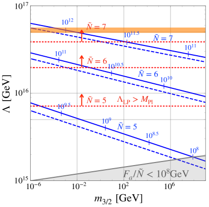
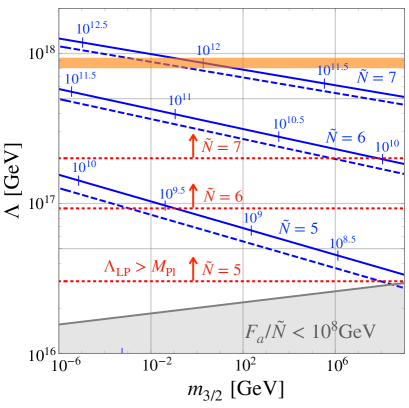
Figure 3: Contours of the quality factor for $\mathcal{Q}=10^{-10}$ (blue solid lines) and $\mathcal{Q}=10^{-12}$ (blue dashed lines) in the $m_{3/2}-\Lambda$ plane. The scales on each blue line denote the decay constant $F_{a}/\tilde{N}$ in the unit of GeV. We take $\iota=1$, $\kappa_{\cancel{\rm PQ}}=1$, $N_{F}=2N-2$, and $\varphi=1$, and utilize the values of $\lambda,\bar{\lambda}$ estimated at the IR fixed point. The dynamical scale is taken as $\Lambda/\Lambda_{\rm mag}=5,100$ in the left and right panels, respectively. The red dotted line represents a lower bound on $\Lambda$ from the Landau pole argument for each $\widetilde{N}\,(=N-2)$. The gray shaded region is excluded by astrophysical bounds. The orange band corresponds to the correct abundance of the axion DM, $\Omega_{a}\simeq\Omega_{\rm CDM}$.

Fig. 3 shows the contours for $\mathcal{Q}=10^{-10}$ (represented by the blue solid lines) and $\mathcal{Q}=10^{-12}$ (blue dashed lines) in the $m_{3/2}-\Lambda$ plane for $\widetilde{N}=5,6,7$ with $N_{F}=2N-2$, i.e. $\widetilde{N}=N-2$. Here, we take $\Lambda/\Lambda_{\rm mag}=5~(100)$ in the left (right) panel and $\iota=\kappa_{\cancel{\rm PQ}}=\varphi=1$, and use the values of $\lambda,\bar{\lambda}$ estimated at the IR fixed point. The scales on each line denote the axion decay constants $F_{a}/\tilde{N}$ in the unit of GeV. The red dotted lines represent the constraint from the Landau pole problem, $\Lambda_{\rm LP}>M_{\rm Pl}$, and for each $N$, it puts a lower bound on $\Lambda$. The gray shaded region corresponds to the astrophysical bounds, $F_{a}/\tilde{N}\lesssim 10^{8}\ {\rm GeV}$ Leinson (2014); Hamaguchi et al. (2018); Leinson (2019); Buschmann et al. (2022); Mayle et al. (1988); Raffelt and Seckel (1988); Turner (1988); Chang et al. (2018); Carenza et al. (2019). Below each blue solid line and above each red dotted line, the quality of $U(1)_{\rm PQ}$ is compatible with the absence of the Landau pole to a sufficiently good degree. In the range of $m_{3/2}$ shown here, the cases of $\widetilde{N}=6,7$ are promising for $\Lambda/\Lambda_{\rm mag}=5$. On the other hand, one can see from the right panel that the quality of the PQ symmetry becomes much higher for a larger $\Lambda/\Lambda_{\rm mag}$. This is because the suppression due to the wavefunction renormalization becomes significant. In this case, the theory with $\widetilde{N}\geq 5$ has the high quality PQ symmetry without a Landau pole problem in a broader range of the gravitino mass, which can be compared with the previous work Nakai and Suzuki (2021) where the gravitino mass is limited below $10\ {\rm GeV}$. In addition, one can see that the $SU(\widetilde{N})$ gauge theory with $\widetilde{N}=5$ becomes viable while it is not in the setup of Ref. Nakagawa et al. (2024).

Let us comment on the value of $\delta$. Although we have mainly shown the results of $\delta=2$, a larger value is also possible, as long as $\widetilde{N}$ is sufficiently large for the theory to be in conformal window. For example, $\widetilde{N}\geq 7$ is required for $\delta=6$. However, we have found that a larger value of $\delta$ does not improve the PQ quality and the Landau pole problem.

V DM axion implications

Our axion model to address the strong CP problem has a viable parameter space consistent with the range of the axion decay constant, $10^{10}\ {\rm GeV}\lesssim F_{a}/\widetilde{N}\lesssim 10^{12}\ {\rm GeV}$, where the axion can give the observed abundance of DM. At the QCD phase transition, the axion DM is produced via the misalignment mechanism Preskill et al. (1983); Abbott and Sikivie (1983); Dine and Fischler (1983). When the PQ symmetry is spontaneously broken before inflation and is never restored after inflation, the axion DM abundance is obtained as Ballesteros et al. (2017)

$$\Omega_{a}h^{2}\simeq 0.14\,\theta_{\rm ini}^{2}\left(\frac{F_{a}/\widetilde{N}}{10^{12}\ {\rm GeV}}\right)^{1.17},$$ (43)

where $\theta_{\rm ini}\equiv a_{\rm ini}/(F_{a}/\widetilde{N})$ is defined as the dimensionless initial position of the axion field. Here we omit the anharmonic effect whose contribution is not significant for the mass range of interest. The abundance can be matched with the observed DM abundance for $F_{a}/\widetilde{N}\simeq 10^{12}\ {\rm GeV}$ and $\theta_{\rm ini}=\mathcal{O}(1)$. The orange band in Fig. 3 shows the region with the correct abundance of DM $(F_{a}/\widetilde{N}\sim 10^{12}\ {\rm GeV})$, which indicates $\widetilde{N}=7,N_{F}=16$, and $m_{3/2}\lesssim 1\ {\rm MeV}~(1\ {\rm GeV})$ for $\Lambda/\Lambda_{\rm mag}=5~(100)$. It is interesting to note that quantum gravity or some other UV effects can leave footprints through the explicit PQ symmetry violation in this region, which will be probed by future neutron EDM experiments, such as the TUCAN, nEDM, n2EDM Ahmed et al. (2019a, b); Ayres et al. (2021).

In the other region of the parameter space, the axion is only a subdominant component of DM. Since our theory is reduced to the MSSM at the electroweak scale, the lightest supersymmetric particle (LSP), such as the neutralino, can become a viable DM candidate, with the conserved $R$-parity Jungman et al. (1996). It is then important to note that our high-quality axion model can accommodate a heavy gravitino, $m_{3/2}\gtrsim 10-100\ {\rm TeV}$, where the mini-split-type SUSY spectrum Ibe and Yanagida (2012); Ibe et al. (2012); Arvanitaki et al. (2013); Arkani-Hamed et al. (2012) can be realized.

Since the axion is very light and acquires quantum fluctuation during inflation, the axionic isocurvature fluctuation imposes an upper bound on the Hubble parameter $H_{\rm inf}$ during inflation Steinhardt and Turner (1983); Axenides et al. (1983); Linde (1985); Seckel and Turner (1985). The isocurvature fluctuation of cold dark matter (CDM) is given by Kobayashi et al. (2013)

$$S_{\rm CDM}\simeq\frac{\delta\rho_{\rm CDM}}{\rho_{\rm CDM}}\simeq\frac{\Omega_{a}}{\Omega_{\rm CDM}}\frac{\delta\rho_{a}}{\rho_{a}}\simeq\frac{\Omega_{a}}{\Omega_{\rm CDM}}\frac{2\delta a_{*}}{a_{*}}\,,$$ (44)

where $\rho_{a(\rm CDM)},\delta\rho_{a(\rm CDM)}$ respectively represent the axion (CDM) energy density and its fluctuation, $\Omega_{a({\rm CDM})}$ is the density parameter for the axion (CDM), and $a_{*},\delta a_{*}$ are the axion field value and its fluctuation during inflation. The third equality uses the fact that $\rho_{a}\propto a_{*}^{2}$. Here the photon fluctuation is ignored with a good approximation, and it is assumed that the isocurvature fluctuation is generated only from the axion. The recent Planck data of anisotropy of cosmic microwave background radiation constrains the isocurvature fluctuation Akrami et al. (2020),

$$\beta_{\rm iso}(k_{*})<0.038\,,$$ (45)

where $\beta_{\rm iso}$ is defined as the ratio between the power spectrum of the adiabatic and isocurvature fluctuations at the scale of $k_{*}=0.05\,{\rm Mpc}^{-1}$. For a natural initial misalignment angle which gives the correct abundance of DM, the upper bound on the scale of inflation is given by

$$H_{\rm inf}\lesssim 2.7\times 10^{7}\ {\rm GeV}\left(\frac{F_{a}/\widetilde{N}}{10^{12}\ {\rm GeV}}\right)^{0.42}.$$ (46)

Compared to the current upper bound from the tensor-to-scalar ratio Akrami et al. (2020), $H_{\rm inf}<6.5\times 10^{13}\ {\rm GeV}$, the upper bound (46) gives a stringent constraint on inflation models.

A possible way out of the axion isocurvature problem is the Linde’s solution Linde (1991) where PQ breaking fields acquire large VEVs during inflation, and the axion fluctuation is significantly suppressed, $\delta\theta_{*}\simeq\widetilde{N}H_{\rm inf}/2\pi M_{\rm Pl}$. In this case, the upper bound on the Hubble parameter during inflation is given by

$$H_{\rm inf}\lesssim 9.1\times 10^{12}\ {\rm GeV}\left(\frac{7}{\widetilde{N}}\right)\left(\frac{10^{12}\ {\rm GeV}}{F_{a}/\widetilde{N}}\right)^{0.59}\!\!\!,$$ (47)

where we use $\Omega_{a}=\Omega_{\rm CDM}$. This is comparable to the current upper bound from the tensor-to-scalar ratio. However, it has been recognized that this mechanism suffers from the enhancement of fluctuations of the PQ breaking scalar fields produced by parametric resonance Kofman et al. (1994). Due to those fluctuations, the PQ symmetry may be restored after inflation, which leads to the domain wall problem Kasuya et al. (1997); Kawasaki et al. (2013); Kawasaki and Sonomoto (2018); Kawasaki et al. (2018).

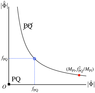
Figure 4: The schematic picture of the minima of the PQ breaking fields $(|\hat{\Phi}|,|\hat{\bar{\Phi}}|)$. The black square at the origin denotes the PQ symmetric point of Eq. (15), and the black line gives the flat direction in Eq. (16). The field $|\hat{\Phi}|$ obtains a large VEV (red bullet) during inflation due to the Hubble induced mass term. When SUSY breaking becomes relevant after inflation, the oscillation along the flat direction starts around the point $(f_{\rm PQ},f_{\rm PQ})$ (blue circle).

Refs. Kasuya et al. (1997); Kawasaki and Sonomoto (2018); Kawasaki et al. (2018) have discussed that a SUSY axion model with a flat direction has a possibility to overcome the shortcoming of the Linde’s solution. The argument can be applied to our axion model with Eq. (16) whose flat direction is deformed by the Hubble induced mass. The scalar potential of $\Phi,\bar{\Phi}$ is then given by

$$V=V_{\mathcal{F}}+V_{\rm soft}+V_{\rm CW}+cH^{2}|\Phi|^{2}+\bar{c}H^{2}|\bar{\Phi}|^{2}\,,$$ (48)

where $H$ denotes the Hubble parameter, and $c,\bar{c}$ are dimensionless constants. The soft SUSY breaking terms do not affect the dynamics during inflation but are relevant to the oscillation after inflation. When we take e.g. $c<0$ and $\bar{c}>0$, $\hat{\Phi},\hat{\bar{\Phi}}$ are expected to acquire VEVs, $v\simeq M_{\rm Pl}$ and $\bar{v}\simeq f_{\rm PQ}^{2}/M_{\rm Pl}$, during inflation, so that the mechanism to suppress the axion fluctuation works well in our model. Fig. 4 shows the schematic picture of the vacuum in the $(|\hat{\Phi}|,|\hat{\bar{\Phi}}|)$ plane, and the VEVs during inflation are denoted by the red bullet on the flat direction (black line). When the oscillation along the flat direction starts around the final vacuum (blue circle) due to SUSY breaking, the fluctuations of the PQ breaking scalar fields are generated via parametric resonance. However, those fluctuations never restore the PQ symmetry. There is a potential issue that the fluctuations make the distribution of the axion field completely flat, which may generate stable domain walls, but it is unlikely because we can expect that a peak of the axion field fluctuation evolves with time due to the axion gradient term. For a further confirmation, numerical simulations are needed Kawasaki and Sonomoto (2018).

VI Discussions

We have explored a new paradigm for the high-quality QCD axion on the basis of electric-magnetic duality in the conformal window of a SUSY gauge theory. The PQ breaking fields emerge in the magnetic picture of the theory. Their large anomalous dimension leads to not only the intermediate scale of the spontaneous PQ violation but also a significant suppression of explicit PQ symmetry breaking operators. The high PQ quality and the absence of a Landau pole in the color gauge coupling are achieved at the same time. The parameter space to realize the correct abundance of the axion DM with the decay constant $f_{a}=10^{10}-10^{12}\ {\rm GeV}$ predicts explicit PQ violation which may be probed by future measurements of the neutron EDM. The axion isocurvature fluctuation can be naturally suppressed by large VEVs of the PQ breaking fields during inflation. In the other viable parameter space, the LSP can become a DM candidate. The model accommodates a heavy gravitino, $m_{3/2}\gtrsim 10-100\ {\rm TeV}$, where the mini-split-type SUSY spectrum is realized. Therefore, our high-quality axion model provides a complete solution to the strong CP problem as well as the identity of DM.

A supersymmetric axion model contains a scalar partner, the saxion, as well as a fermionic partner called the axino. In Sec. II.4, we have discussed the stabilization of the saxion with SUSY breaking effects, and it was found that its mass is given by the soft mass scale $\sim 1\ {\rm TeV}$. Such a saxion mode can easily decay into gluons so that any cosmological problem is not induced. On the other hand, the axino can acquire a mass $m_{\widetilde{a}}=\mathcal{O}(m_{3/2})$ from supergravity effects, $\mathcal{L}\supset\int d^{4}\theta(A+A^{\dagger})(X+X^{\dagger})/M_{\rm Pl}$, where $A$ and $X$ respectively denote the axion and SUSY breaking superfields. Cosmologically, the overproduction of the axino puts an upper bound on the reheating temperature in some range of $m_{3/2}$ Cheung et al. (2012).

References

- Baker et al. (2006) C. A. Baker et al., Phys. Rev. Lett. 97, 131801 (2006), arXiv:hep-ex/0602020 .
- Pendlebury et al. (2015) J. M. Pendlebury et al., Phys. Rev. D 92, 092003 (2015), arXiv:1509.04411 [hep-ex] .
- Peccei and Quinn (1977) R. D. Peccei and H. R. Quinn, Phys. Rev. Lett. 38, 1440 (1977).
- Weinberg (1978) S. Weinberg, Phys. Rev. Lett. 40, 223 (1978).
- Wilczek (1978) F. Wilczek, Phys. Rev. Lett. 40, 279 (1978).
- Preskill et al. (1983) J. Preskill, M. B. Wise, and F. Wilczek, Phys. Lett. B 120, 127 (1983).
- Abbott and Sikivie (1983) L. F. Abbott and P. Sikivie, Phys. Lett. B 120, 133 (1983).
- Dine and Fischler (1983) M. Dine and W. Fischler, Phys. Lett. B 120, 137 (1983).
- Mayle et al. (1988) R. Mayle, J. R. Wilson, J. R. Ellis, K. A. Olive, D. N. Schramm, and G. Steigman, Phys. Lett. B 203, 188 (1988).
- Raffelt and Seckel (1988) G. Raffelt and D. Seckel, Phys. Rev. Lett. 60, 1793 (1988).
- Turner (1988) M. S. Turner, Phys. Rev. Lett. 60, 1797 (1988).
- Chang et al. (2018) J. H. Chang, R. Essig, and S. D. McDermott, JHEP 09, 051 (2018), arXiv:1803.00993 [hep-ph] .
- Carenza et al. (2019) P. Carenza, T. Fischer, M. Giannotti, G. Guo, G. Martínez-Pinedo, and A. Mirizzi, JCAP 10, 016 (2019), [Erratum: JCAP 05, E01 (2020)], arXiv:1906.11844 [hep-ph] .
- Leinson (2014) L. B. Leinson, JCAP 08, 031 (2014), arXiv:1405.6873 [hep-ph] .
- Hamaguchi et al. (2018) K. Hamaguchi, N. Nagata, K. Yanagi, and J. Zheng, Phys. Rev. D 98, 103015 (2018), arXiv:1806.07151 [hep-ph] .
- Leinson (2019) L. B. Leinson, JCAP 11, 031 (2019), arXiv:1909.03941 [hep-ph] .
- Buschmann et al. (2022) M. Buschmann, C. Dessert, J. W. Foster, A. J. Long, and B. R. Safdi, Phys. Rev. Lett. 128, 091102 (2022), arXiv:2111.09892 [hep-ph] .
- O’Hare (2020) C. O’Hare, “cajohare/axionlimits: Axionlimits,” https://cajohare.github.io/AxionLimits/ (2020).
- Dine and Seiberg (1986) M. Dine and N. Seiberg, Nucl. Phys. B 273, 109 (1986).
- Barr and Seckel (1992) S. M. Barr and D. Seckel, Phys. Rev. D 46, 539 (1992).
- Kamionkowski and March-Russell (1992a) M. Kamionkowski and J. March-Russell, Phys. Lett. B 282, 137 (1992a), arXiv:hep-th/9202003 .
- Kamionkowski and March-Russell (1992b) M. Kamionkowski and J. March-Russell, Phys. Rev. Lett. 69, 1485 (1992b), arXiv:hep-th/9201063 .
- Holman et al. (1992) R. Holman, S. D. H. Hsu, T. W. Kephart, E. W. Kolb, R. Watkins, and L. M. Widrow, Phys. Lett. B 282, 132 (1992), arXiv:hep-ph/9203206 .
- Kallosh et al. (1995) R. Kallosh, A. D. Linde, D. A. Linde, and L. Susskind, Phys. Rev. D 52, 912 (1995), arXiv:hep-th/9502069 .
- Carpenter et al. (2009a) L. M. Carpenter, M. Dine, and G. Festuccia, Phys. Rev. D 80, 125017 (2009a), arXiv:0906.1273 [hep-th] .
- Carpenter et al. (2009b) L. M. Carpenter, M. Dine, G. Festuccia, and L. Ubaldi, Phys. Rev. D 80, 125023 (2009b), arXiv:0906.5015 [hep-th] .
- Banks and Seiberg (2011) T. Banks and N. Seiberg, Phys. Rev. D 83, 084019 (2011), arXiv:1011.5120 [hep-th] .
- Witten (2018) E. Witten, Nature Phys. 14, 116 (2018), arXiv:1710.01791 [hep-th] .
- Harlow and Ooguri (2019) D. Harlow and H. Ooguri, Phys. Rev. Lett. 122, 191601 (2019), arXiv:1810.05337 [hep-th] .
- Harlow and Ooguri (2021) D. Harlow and H. Ooguri, Commun. Math. Phys. 383, 1669 (2021), arXiv:1810.05338 [hep-th] .
- Kim (1985) J. E. Kim, Phys. Rev. D 31, 1733 (1985).
- Choi and Kim (1985) K. Choi and J. E. Kim, Phys. Rev. D 32, 1828 (1985).
- Randall (1992) L. Randall, Phys. Lett. B 284, 77 (1992).
- Izawa et al. (2002) K. I. Izawa, T. Watari, and T. Yanagida, Phys. Lett. B 534, 93 (2002), arXiv:hep-ph/0202171 .
- Yamada et al. (2016) M. Yamada, T. T. Yanagida, and K. Yonekura, Phys. Rev. Lett. 116, 051801 (2016), arXiv:1510.06504 [hep-ph] .
- Redi and Sato (2016) M. Redi and R. Sato, JHEP 05, 104 (2016), arXiv:1602.05427 [hep-ph] .
- Di Luzio et al. (2017) L. Di Luzio, E. Nardi, and L. Ubaldi, Phys. Rev. Lett. 119, 011801 (2017), arXiv:1704.01122 [hep-ph] .
- Lillard and Tait (2017) B. Lillard and T. M. P. Tait, JHEP 11, 005 (2017), arXiv:1707.04261 [hep-ph] .
- Lillard and Tait (2018) B. Lillard and T. M. P. Tait, JHEP 11, 199 (2018), arXiv:1811.03089 [hep-ph] .
- Gavela et al. (2019) M. B. Gavela, M. Ibe, P. Quilez, and T. T. Yanagida, Eur. Phys. J. C 79, 542 (2019), arXiv:1812.08174 [hep-ph] .
- Lee and Yin (2019) H.-S. Lee and W. Yin, Phys. Rev. D 99, 015041 (2019), arXiv:1811.04039 [hep-ph] .
- Yamada and Yanagida (2021) M. Yamada and T. T. Yanagida, Phys. Lett. B 816, 136267 (2021), arXiv:2101.10350 [hep-ph] .
- Ishida et al. (2022) H. Ishida, S. Matsuzaki, and X.-C. Peng, Eur. Phys. J. C 82, 107 (2022), arXiv:2103.13644 [hep-ph] .
- Contino et al. (2022) R. Contino, A. Podo, and F. Revello, JHEP 04, 180 (2022), arXiv:2112.09635 [hep-ph] .
- Nakai and Suzuki (2021) Y. Nakai and M. Suzuki, Phys. Lett. B 816, 136239 (2021), arXiv:2102.01329 [hep-ph] .
- Nakagawa et al. (2024) S. Nakagawa, Y. Nakai, M. Yamada, and Y. Zhang, Phys. Lett. B 849, 138447 (2024), arXiv:2309.06964 [hep-ph] .
- Flacke et al. (2007) T. Flacke, B. Gripaios, J. March-Russell, and D. Maybury, JHEP 01, 061 (2007), arXiv:hep-ph/0611278 .
- Cox et al. (2020) P. Cox, T. Gherghetta, and M. D. Nguyen, JHEP 01, 188 (2020), arXiv:1911.09385 [hep-ph] .
- Bonnefoy et al. (2021) Q. Bonnefoy, P. Cox, E. Dudas, T. Gherghetta, and M. D. Nguyen, JHEP 04, 084 (2021), arXiv:2012.09728 [hep-ph] .
- Lee et al. (2022) S. J. Lee, Y. Nakai, and M. Suzuki, JHEP 03, 038 (2022), arXiv:2112.08083 [hep-ph] .
- Rubakov (1997) V. A. Rubakov, JETP Lett. 65, 621 (1997), arXiv:hep-ph/9703409 .
- Berezhiani et al. (2001) Z. Berezhiani, L. Gianfagna, and M. Giannotti, Phys. Lett. B 500, 286 (2001), arXiv:hep-ph/0009290 .
- Hook (2015) A. Hook, Phys. Rev. Lett. 114, 141801 (2015), arXiv:1411.3325 [hep-ph] .
- Fukuda et al. (2015) H. Fukuda, K. Harigaya, M. Ibe, and T. T. Yanagida, Phys. Rev. D 92, 015021 (2015), arXiv:1504.06084 [hep-ph] .
- Gherghetta et al. (2016) T. Gherghetta, N. Nagata, and M. Shifman, Phys. Rev. D 93, 115010 (2016), arXiv:1604.01127 [hep-ph] .
- Dimopoulos et al. (2016) S. Dimopoulos, A. Hook, J. Huang, and G. Marques-Tavares, JHEP 11, 052 (2016), arXiv:1606.03097 [hep-ph] .
- Gherghetta and Nguyen (2020) T. Gherghetta and M. D. Nguyen, JHEP 12, 094 (2020), arXiv:2007.10875 [hep-ph] .
- Alves and Weiner (2018) D. S. M. Alves and N. Weiner, JHEP 07, 092 (2018), arXiv:1710.03764 [hep-ph] .
- Liu et al. (2021) J. Liu, N. McGinnis, C. E. M. Wagner, and X.-P. Wang, JHEP 05, 138 (2021), arXiv:2102.10118 [hep-ph] .
- Girmohanta et al. (2024) S. Girmohanta, S. Nakagawa, Y. Nakai, and J. Xu, JHEP 10, 153 (2024), arXiv:2405.13425 [hep-ph] .
- Cheng and Kaplan (2001) H.-C. Cheng and D. E. Kaplan, (2001), arXiv:hep-ph/0103346 .
- Harigaya et al. (2013) K. Harigaya, M. Ibe, K. Schmitz, and T. T. Yanagida, Phys. Rev. D 88, 075022 (2013), arXiv:1308.1227 [hep-ph] .
- Fukuda et al. (2017) H. Fukuda, M. Ibe, M. Suzuki, and T. T. Yanagida, Phys. Lett. B 771, 327 (2017), arXiv:1703.01112 [hep-ph] .
- Fukuda et al. (2018) H. Fukuda, M. Ibe, M. Suzuki, and T. T. Yanagida, JHEP 07, 128 (2018), arXiv:1803.00759 [hep-ph] .
- Ibe et al. (2018) M. Ibe, M. Suzuki, and T. T. Yanagida, JHEP 08, 049 (2018), arXiv:1805.10029 [hep-ph] .
- Choi et al. (2020) G. Choi, M. Suzuki, and T. T. Yanagida, JHEP 07, 048 (2020), arXiv:2005.10415 [hep-ph] .
- Yin (2020) W. Yin, JHEP 10, 032 (2020), arXiv:2007.13320 [hep-ph] .
- Chen et al. (2021) N. Chen, Y. Liu, and Z. Teng, Phys. Rev. D 104, 115011 (2021), arXiv:2106.00223 [hep-ph] .
- Seiberg (1995) N. Seiberg, Nucl. Phys. B 435, 129 (1995), arXiv:hep-th/9411149 .
- Csáki et al. (2024) C. Csáki, R. Ovadia, M. Ruhdorfer, O. Telem, and J. Terning, (2024), arXiv:2411.15312 [hep-ph] .
- Seiberg and Witten (1994) N. Seiberg and E. Witten, Nucl. Phys. B 426, 19 (1994), [Erratum: Nucl.Phys.B 430, 485–486 (1994)], arXiv:hep-th/9407087 .
- Intriligator and Seiberg (2007) K. A. Intriligator and N. Seiberg, Class. Quant. Grav. 24, S741 (2007), arXiv:hep-ph/0702069 .
- ’t Hooft (1980) G. ’t Hooft, NATO Sci. Ser. B 59, 135 (1980).
- Kim (1979) J. E. Kim, Phys. Rev. Lett. 43, 103 (1979).
- Shifman et al. (1980) M. A. Shifman, A. I. Vainshtein, and V. I. Zakharov, Nucl. Phys. B 166, 493 (1980).
- Workman et al. (2022) R. L. Workman et al. (Particle Data Group), PTEP 2022, 083C01 (2022).
- Staub (2008) F. Staub, (2008), arXiv:0806.0538 [hep-ph] .
- Coleman and Weinberg (1973) S. R. Coleman and E. J. Weinberg, Phys. Rev. D 7, 1888 (1973).
- Grilli di Cortona et al. (2016) G. Grilli di Cortona, E. Hardy, J. Pardo Vega, and G. Villadoro, JHEP 01, 034 (2016), arXiv:1511.02867 [hep-ph] .
- Abel et al. (2020) C. Abel et al., Phys. Rev. Lett. 124, 081803 (2020), arXiv:2001.11966 [hep-ex] .
- Ballesteros et al. (2017) G. Ballesteros, J. Redondo, A. Ringwald, and C. Tamarit, JCAP 08, 001 (2017), arXiv:1610.01639 [hep-ph] .
- Ahmed et al. (2019a) S. Ahmed et al. (TUCAN), Phys. Rev. C 99, 025503 (2019a), arXiv:1809.04071 [physics.ins-det] .
- Ahmed et al. (2019b) M. W. Ahmed et al. (nEDM), JINST 14, P11017 (2019b), arXiv:1908.09937 [physics.ins-det] .
- Ayres et al. (2021) N. J. Ayres et al. (n2EDM), Eur. Phys. J. C 81, 512 (2021), arXiv:2101.08730 [physics.ins-det] .
- Jungman et al. (1996) G. Jungman, M. Kamionkowski, and K. Griest, Phys. Rept. 267, 195 (1996), arXiv:hep-ph/9506380 .
- Ibe and Yanagida (2012) M. Ibe and T. T. Yanagida, Phys. Lett. B 709, 374 (2012), arXiv:1112.2462 [hep-ph] .
- Ibe et al. (2012) M. Ibe, S. Matsumoto, and T. T. Yanagida, Phys. Rev. D 85, 095011 (2012), arXiv:1202.2253 [hep-ph] .
- Arvanitaki et al. (2013) A. Arvanitaki, N. Craig, S. Dimopoulos, and G. Villadoro, JHEP 02, 126 (2013), arXiv:1210.0555 [hep-ph] .
- Arkani-Hamed et al. (2012) N. Arkani-Hamed, A. Gupta, D. E. Kaplan, N. Weiner, and T. Zorawski, (2012), arXiv:1212.6971 [hep-ph] .
- Steinhardt and Turner (1983) P. J. Steinhardt and M. S. Turner, Phys. Lett. B 129, 51 (1983).
- Axenides et al. (1983) M. Axenides, R. H. Brandenberger, and M. S. Turner, Phys. Lett. B 126, 178 (1983).
- Linde (1985) A. D. Linde, Phys. Lett. B 158, 375 (1985).
- Seckel and Turner (1985) D. Seckel and M. S. Turner, Phys. Rev. D 32, 3178 (1985).
- Kobayashi et al. (2013) T. Kobayashi, R. Kurematsu, and F. Takahashi, JCAP 09, 032 (2013), arXiv:1304.0922 [hep-ph] .
- Akrami et al. (2020) Y. Akrami et al. (Planck), Astron. Astrophys. 641, A10 (2020), arXiv:1807.06211 [astro-ph.CO] .
- Linde (1991) A. D. Linde, Phys. Lett. B 259, 38 (1991).
- Kofman et al. (1994) L. Kofman, A. D. Linde, and A. A. Starobinsky, Phys. Rev. Lett. 73, 3195 (1994), arXiv:hep-th/9405187 .
- Kasuya et al. (1997) S. Kasuya, M. Kawasaki, and T. Yanagida, Phys. Lett. B 409, 94 (1997), arXiv:hep-ph/9608405 .
- Kawasaki et al. (2013) M. Kawasaki, T. T. Yanagida, and K. Yoshino, JCAP 11, 030 (2013), arXiv:1305.5338 [hep-ph] .
- Kawasaki and Sonomoto (2018) M. Kawasaki and E. Sonomoto, Phys. Rev. D 97, 083507 (2018), arXiv:1710.07269 [hep-ph] .
- Kawasaki et al. (2018) M. Kawasaki, E. Sonomoto, and T. T. Yanagida, Phys. Lett. B 782, 181 (2018), arXiv:1801.07409 [hep-ph] .
- Cheung et al. (2012) C. Cheung, G. Elor, and L. J. Hall, Phys. Rev. D 85, 015008 (2012), arXiv:1104.0692 [hep-ph] .