Fully Bayesian Wideband Direction-of-Arrival
Estimation and Detection via RJMCMC

Abstract

We propose a fully Bayesian approach to wideband, or broadband, direction-of-arrival (DoA) estimation and signal detection. Unlike previous works in wideband DoA estimation and detection, where the signals were modeled in the time-frequency domain, we directly model the time-domain representation and treat the non-causal part of the source signal as latent variables. Furthermore, our Bayesian model allows for closed-form marginalization of the latent source signals by leveraging conjugacy. To further speed up computation, we exploit the sparse “stripe matrix structure” of the considered system, which stems from the circulant matrix representation of linear time-invariant (LTI) systems. This drastically reduces the time complexity of computing the likelihood from $\mathcal{O}(N^{3}k^{3})$ to $\mathcal{O}(Nk^{3})$, where $N$ is the number of samples received by the array and $k$ is the number of sources. These computational improvements allow for efficient posterior inference through reversible jump Markov chain Monte Carlo (RJMCMC). We use the non-reversible extension of RJMCMC (NRJMCMC), which often achieves lower autocorrelation and faster convergence than the conventional reversible variant. Detection, estimation, and reconstruction of the latent source signals can then all be performed in a fully Bayesian manner through the samples drawn using NRJMCMC. We evaluate the detection performance of the procedure by comparing against generalized likelihood ratio testing (GLRT) and information criteria.

I Introduction

DDirection-of-arrival (DoA) estimation is a problem of estimating the incoming direction of unknown localized signals using an array of sensors (or receivers). It is a central problem in various application areas, such as mobile communication, passive sonar, seismology, and radar-based target detection. Since the emergence of array signal processing, DoA estimation has been studied extensively [1, 2, 3]. Closely related is signal detection [1, §3.14.7], where, given a noisy recording, the problem is to determine how many signals are emitted by distinct sources (or “targets”). For array signals, this is inherently intertwined with estimation since we cannot detect a signal without knowing where to look. Furthermore, determining whether a signal is present or not asks the more fundamental question of “What constitutes a signal?” This makes detection more challenging than estimation, requiring stronger modeling assumptions. In statistical terms, this corresponds to a (nested) model selection or model order determination problem [4, 5, 6].

Under the narrowband signal model [2], the detection problem has been successfully tackled through various approaches from information-theoretic methods [7, 8], hypothesis testing [9, 10, 11, 12, 13], and Bayesian model comparison [14, 15]. For some applications, however, the signals of interest may lie in different bands or span multiple frequency bands, meaning that narrowband methods are no longer applicable (e.g. passive sonar [16, 17]). For these applications, wideband methods have to be applied.

Wideband, also called broadband, DoA estimation and detection methods [1, Ch. 14.6] avoid relying on the narrowband assumption by directly dealing with the wideband nature of wideband signals. Earlier attempts tried to focus the multiple frequency bands into a single reference narrowband [7, 18, 19, 20]. These so-called focused subspace methods were popular as they allow for the use of off-the-shelf narrowband detection methods, typically information-theoretic approaches [8, 5], on the reference band [18]. Unfortunately, focused subspace methods require an accurate initial guess of the number of sources and their DoAs [21, 22], resulting in a chicken-and-egg problem that complicates their use. Furthermore, information-theoretic methods, or “information criteria,” are known to achieve limited performance in the low SNR, low snapshot regime [15, 23, 13].

Most of the issues with focused subspace approaches stem from the fundamental concept of collapsing multiple frequency bins into one. In contrast, maximum likelihood (ML; [1, §3.14.6.1], [24]) approaches rigorously model wideband signals and are known to outperform subspace methods “when the signal-to-noise ratio is small, or alternatively, when the number of samples (“snapshots”) is small” [25]. Moreover, ML methods enable detection through generalized likelihood ratio testing (GLRT; [4, §3.02.3.2]). That is, detection is now viewed as a multiple hypothesis testing problem where, given the null hypothesis $H_{k}$ that $k$ targets are present, the alternative composite hypothesis $H_{k+1}$ that at least $k+1$ targets are present is tested for each $k\in\{0,\ldots,k_{\mathrm{max}}\}$ ($k_{\mathrm{max}}$ is the assumed maximum number of targets). For wideband signals with additive white Gaussian noise, test statistics have been derived by [26], where boostrapping [27] has been used to compute the $p$-values needed for the tests [28, 23].

While GLRT resolves the limitations of focused subspace approaches, it suffers from the usual limitations of hypothesis testing: Most hypothesis testing schemes are designed to control the long-term false positive rate (Type-I error rate) at the cost of a higher false negative rate (Type-II error rate) [29, §8.3]. Therefore, when accuracy or having a low false negative rate (“power”) is also of interest, the design principles of hypothesis testing become misaligned. This problem is further exacerbated in signal detection, as it is typically approached as a multiple-testing problem [4]. When controlling the Type-I error, the power of a multiple hypothesis test decreases as the number of considered hypotheses ($k_{\mathrm{max}}$) increases.

On the other hand, the Bayesian approach to model comparison [30, 31] is immune to these issues [32]. In fact, the Bayesian approach can select the model that maximizes model selection accuracy. More precisely, assuming the model is well specified, Bayesian point estimators achieve the optimal average performance (Bayes risk) for any given target performance metric [32, Thm 2.3.2]. For signal processing problems, reversible jump Markov chain Monte Carlo (RJMCMC; [33, 34]), also known as transdimensional MCMC [35, 36], often enables inference of the model posterior and their corresponding parameter posteriors all at once, and have been successfully applied to various signal processing problems  [37, 38, 39, 40, 41, 42, 43], including narrowband [14] and wideband [44] DoA estimation and detection.

For wideband DoA estimation and detection, Ng et al. [44] have previously proposed a Bayesian approach that leveraged RJMCMC. However, their model formulation resulted in an intractable posterior over the source signals. As such, they relied on a plug-in estimate for the source signals obtained through a recursive maximum a posteriori (MAP) procedure. Naturally, this violates the likelihood principle and ignores our uncertainty about the latent source signals.

This work instead provides an alternative Bayesian probabilistic model for wideband DoA estimation and detection that is fully Bayesian and generally applicable. Compared to typical wideband signal models, which model the time-frequency spectrum [1, §14.6], and the model by [44], our probabilistic model has the following features:

• We model the signal propagation using a conjugate symmetric linear time-invariant (LTI) filter. Specifically, we leverage the fractional delay filter by Pei and Lai [45] and its later extension [46]. This allows for the real-valued reconstruction of the latent source signals (Section III-A).

• Our Bayesian formulation of the signal model allows for closed-form marginalization of the latent source signals and the signal power parameters. For $k$ sources, $N$ received measurements, and an $L$-tap FIR filter representing the signal propagation, marginalization reduces the number of parameters needed to be inferred from $k(N+L-1)+2k+1$ to $2k$ (Section III-B).

• We exploit the frequency domain representation of LTI filters to reduce the computational complexity. In particular, we exploit the sparse “stripe matrix” structure (Appendix A) of the system, enabling computation of the likelihood in $\mathcal{O}(Nk^{3})$ operations (Section IV-B).

Our overall detection and estimation procedure is described in Section IV-A. For inference, we leverage the non-reversible variant of RJMCMC proposed by Gagnon and Doucet [47], which achieves lower autocorrelation compared to conventional reversible implementations (Section IV-C). We evaluate the detection performance of our proposed Bayesian detecting procedure in Section V.

II Background

Notation

We denote vectors in bold small letters (e.g., $\mathbfit{x},\mathbfit{y}$); matrices in bold capitals (e.g., $\mathbfit{A},\mathbfit{B}$); $\mathbf{I}_{N}\in\mathbb{R}^{N\times N}$ is the identity matrix; $\mathbf{O}_{N}\in\mathbb{R}^{N\times N}$ is a zero matrix; $\mathbf{0}_{N}\in\mathbb{R}^{N}$ is a vector of $N$ zeros. $\mathbfit{A}^{\dagger}$ is the Hermitian of $\mathbfit{A}$; $\circledast$ is the discrete circular convolution; $\mathrm{j}\triangleq\sqrt{-1}$ is the imaginary number. For a discrete-time signal $x_{i}[0],\ldots,x_{i}[N\text{-}1]$ for some $N\in\mathbb{N}_{>0}$, omitting the index implies concatenation over the sample index such that $\mathbfit{x}_{i}=\left(x_{i}[0],\ldots,x_{i}[N\text{-}1]\right)$. For a collection of signals $\mathbfit{x}_{1},\ldots,\mathbfit{x}_{k}$, omitting the subscript or using a “range” as $1\text{:}k$ implies concatenation over the collection, $\mathbfit{x}[n]=\mathbfit{x}_{1\text{:}k}[n]=\left(x_{1}[n],\,\ldots,\,x_{k}[n]\right)$ and $\mathbfit{x}=\mathbfit{x}_{1\text{:}k}=\left(\mathbfit{x}_{1},\ldots,\mathbfit{x}_{k}\right)$. Lastly, a range of indices from 1 to $N$ is denoted as $[N]\triangleq\{1,\ldots,N\}$.

II-A Wideband Signal Models

We will first discuss the signal models typically used for modeling wideband signals [1].

Continuous-Time Model

Consider an $M$ sensor array with continuous-time measurements. The measurement, or sample, $y_{i}\left(t\right)$ received by the $i$th sensor at time $t\geq 0$ is

$$y_{i}\left(t\right)={\textstyle\sum}^{k}_{j=1}x_{j}\left(t-\Delta_{i}\left(\phi_{j}\right)\right)+\eta_{i}\left(t\right),\text{ where }$$ (1)

$\Delta_{i}\left(\phi_{j}\right)\in\mathbb{R}$	is the inter-sensor delay for a signal impinging to the $i$th sensor from an angle of $\phi_{j}\in\left[\nicefrac{{-\rm\pi}}{{2}},\nicefrac{{\rm\pi}}{{2}}\right]$,
$x_{j}\left(t\right)\in\mathbb{R}$	is signal emitted by the $j$th source, and
$\eta_{i}\left(t\right)\in\mathbb{R}^{M}$	is the noise and interference.

In the DoA estimation problem the source signals ${\{x_{j}\left(t\right)\}}_{j\in[k]}$, and noise and interference ${\{\eta_{1}\left(t\right)\}}_{j\in[M]}$ are all assumed to be unknown, and in the signal detection problem, the number of sources, or model order, $k$, is also unknown. Note that the fact that we assume real-value signals means that we impose conjugate symmetry constraints [48, §2.8] on the model. This is without loss of generality, as our derivations can be generalized to complex signals.

Discrete Time-Frequency Model

There are multiple ways to interpret the model in Eq. 1 in discrete time. Previous works utilized the frequency domain representation of Eq. 1. That is, for each channel $i\in[M]$, the received signal $\mathbfit{y}_{i}$ is processed through the short-time Fourier transform (STFT) with non-overlapping “snapshots” such that $y_{i}[b,s]$ is its $b$th frequency bin and $s$th snapshot. For $N=S\cdot B$ received samples, the STFT yields $S$ snapshots and $B$ frequency bins. Then, for $(s,b)\in[S]\times[B]$, the channel-wise concatenation $\mathbfit{y}[s,b]\in\mathbb{C}^{M}$ is modeled as

$$\mathbfit{y}\left[s,b\right]={\textstyle\sum^{k}_{j=1}}\mathbfit{a}\left(f_{b},\phi_{j}\right)x_{j}\left[s,b\right]+\mathbfit{\eta}\left[s,b\right],$$ (2)

where $\mathbfit{a}\left(f_{b},\phi_{j}\right)\in\mathbb{C}^{M}$ is a “steering vector” defined as

$$\mathbfit{a}\left(f_{b},\phi_{j}\right)\triangleq{\begin{bmatrix}\mathrm{e}^{-\mathrm{j}2\mathrm{\pi}f_{b}\Delta_{1}\left(\phi_{j}\right)}&\ldots&\mathrm{e}^{-\mathrm{j}2\mathrm{\pi}f_{b}\Delta_{M}\left(\phi_{j}\right)}\end{bmatrix}}^{\top}.$$ (3)

For a uniform linear array (ULA), the inter-sensor delay is typically set as $\Delta_{i}\left(\phi_{j}\right)\triangleq-\left(i-1\right)d\sin\left(\theta_{j}\right)/c$, where $c$ is the propagation speed of the medium (e.g., speed of sound in the case of acoustic signals) and $d$ is the sensor displacement.

The model in Eq. 2 has been widely used [1, §3.14.6.1]. However, it has some limitations: First, the steering vector $\mathbfit{a}\left(f_{b},\phi_{j}\right)$ is not conjugate symmetric when the delay $\Delta_{i}\left(\phi_{j}\right)\cdot f_{s}$ is fractional, meaning that it fails to model real-valued signals [48, §2.8]. Second, modeling the STFT forces us to reason about frequency resolution and temporal resolution, which shouldn’t inherently be necessary for DoA estimation. This work proposes an alternative, pure time domain modeling approach that uses the frequency-domain perspective to speed up computation.

III Bayesian Modeling

III-A Time Domain Wideband Signal Model

Non-Causal Discrete-Time Model

Recall the ideal continuous time model in Eq. 1. We will represent the time delay with an $L$-tap conjugate symmetric finite impulse response (FIR) filter, where $L\in\mathbb{N}_{>0}$ is assumed to be an odd number for convenience. Let the propagation of the signal emitted by the $j$th source to the $i$th sensor be represented as $h_{i,j}\triangleq h_{i}\left(\phi_{j}\right)$, where $i\in[M]$ and $j\in[k]$. $h_{i,j}$ is assumed to be non-causally centered at $n=0$ such that, if there is no delay, $h_{i,j}[n]=\delta[n]$. Then, for $n\in\{0,\,\ldots,\,N-1\}$, the signal received by the $i$th sensor can be modeled as

$$y_{i}\left[n\right] =\sum^{k}_{j=1}\left(\sum_{l=-\lfloor{\nicefrac{{L}}{{2}}}\rfloor}^{\lfloor{\nicefrac{{L}}{{2}}}\rfloor}h_{i,j}\left[l\right]x_{j}\left[n-l\right]\right)+\eta_{i}\left[n\right].$$ (4)

Notice that, to utilize all $N$ measurements, the source signals have to be defined on the interval $n\in\{-\lfloor\nicefrac{{L}}{{2}}\rfloor,\,\ldots,\,N+\lfloor\nicefrac{{L}}{{2}}\rfloor\}$.

Periodic Discrete-Time Model

Even though Eq. 4 is non-causal, it is realizable by wrapping around, or “aliasing,” the non-causal part. This can be done by treating $x_{j}$ and $h_{i,j}$ as periodic signals with period $N^{\prime}\triangleq N+L-1$ such that

$$y_{i}\left[n\right]=\sum^{k}_{j=1}\left(\sum_{l=0}^{N^{\prime}-1}h^{\prime}_{i,j}\left[l\right]x_{j}\left[{\left(n-l\right)}_{\mathrm{mod}\;N^{\prime}}\right]\right)+\eta_{i}\left[n\right],$$

where $h^{\prime}_{i,j}:[N^{\prime}]\to\mathbb{R}$ is $h_{i,j}$ padded to the right with $N$ zeros and the non-causal part wrapped around such that

$$h^{\prime}_{i,j}[n]\triangleq\begin{cases}h_{i,j}[n]&\text{if $0\leq n\leq\lfloor\nicefrac{{L}}{{2}}\rfloor$}\\ 0&\text{if $\lfloor\nicefrac{{L}}{{2}}\rfloor+1\leq n\leq N+\lfloor\nicefrac{{L}}{{2}}\rfloor-1$}\\ h_{i,j}[n\text{-}N\text{-}L\text{+}1]&\text{otherwise}.\end{cases}$$ (5)

This corresponds to the circular convolution [48, §8.6.5]

$$y_{i}\left[n\right] ={\sum^{k}_{j=1}}\left(h^{\prime}_{i,j}\circledast x_{j}\right)\left[n\right]+\eta_{i}\left[n\right]$$ (6)

Note that, as we did not pad $x_{j}$, this is not the usual circular convolution realization of the linear convolution as in [48, §8.7]. Instead, we are assuming that the length of the source signal $\mathbfit{x}$ is longer than the received signal depending on $L$. Compared to the more classical causal realization technique of introducing group delay [48, §5.5], this aliasing-based technique is computationally convenient under the discrete Fourier transform (DFT), as we will demonstrate in Section IV-B.

Linear System Representation

Since $h^{\prime}_{i,j}$ is a periodic FIR filter, it has a circulant matrix representation $\mathbfit{H}_{i,j}\triangleq\mathbfit{H}_{i}\left(\phi_{j}\right)\in\mathbb{R}^{N^{\prime}\times N^{\prime}}$ [49], which can be applied to Eq. 6 as

$$\mathbfit{y}_{i}={\sum_{j=1}^{k}}\mathbfit{M}\mathbfit{H}_{i,j}\,\mathbfit{x}_{j}+\mathbfit{\eta},$$ (7)

where $\mathbfit{M}\triangleq{\begin{bmatrix}\mathbf{I}_{N}&\mathbf{O}_{L-1}\end{bmatrix}}\in\mathbb{R}^{N\times N^{\prime}}$ is a “truncation matrix” truncating the last $L-1$ dimensions.

We can denote this as one big linear system:

$$\begin{bmatrix}\mathbfit{y}_{1}\\ \mathbfit{y}_{2}\\ \vdots\\ \mathbfit{y}_{M}\end{bmatrix}=\begin{bmatrix}\mathbfit{M}\mathbfit{H}_{1,1}&\mathbfit{M}\mathbfit{H}_{1,2}&\ldots&\mathbfit{M}\mathbfit{H}_{1,k}\\ \mathbfit{M}\mathbfit{H}_{2,1}&\mathbfit{M}\mathbfit{H}_{2,2}&&\mathbfit{M}\mathbfit{H}_{2,k}\\ \vdots&&\ddots&\vdots\\ \mathbfit{M}\mathbfit{H}_{M,1}&\mathbfit{M}\mathbfit{H}_{M,2}&\ldots&\mathbfit{M}\mathbfit{H}_{M,k}\end{bmatrix}\begin{bmatrix}\mathbfit{x}_{1}\\ \mathbfit{x}_{2}\\ \vdots\\ \mathbfit{x}_{k}\end{bmatrix}+\mathbfit{\eta}.$$ (8)

Denoting the block-wise truncation as $\mathbfit{M}_{M}\triangleq\mathrm{block\text{-}diagonal}_{M}\left(\mathbfit{M},\ldots,\mathbfit{M}\right)$ and the filters as $\mathbfit{H}\left(\mathbfit{\phi}_{1\text{:}k}\right)\triangleq\mathbfit{H}_{1\text{:}M,1\text{:}k}$, the resulting linear system is

$$\mathbfit{y}=\mathbfit{A}\left(\mathbfit{\phi}_{1\text{:}k}\right)\,\mathbfit{x}_{1\text{:}k}+\mathbfit{\eta},$$ (9)

where $\mathbfit{A}\left(\mathbfit{\phi}_{1\text{:}k}\right)\triangleq\mathbfit{M}_{M}\mathbfit{H}\left(\mathbfit{\phi}_{1\text{:}k}\right):\mathbb{R}^{k}\rightarrow\mathbb{R}^{MN\times kN^{\prime}}$, $\mathbfit{y}\in\mathbb{R}^{MN}$, $\mathbfit{x}_{1\text{:}k}\in\mathbb{R}^{kN^{\prime}}$. The system in Eq. 9 is quite large, and attempts to solve the system directly will be computationally infeasible. In Section IV-B, we will demonstrate how to speed up computation by leveraging the circulant structure of $\mathbfit{H}_{i,j}$.

Time Delay Filter

Recall that the time-delay filter $h^{\prime}_{i,j}$ is an $L$-tap non-causal filter zero-padded into an $N^{\prime}$-tap periodic filter. For our implementation, we directly used a $N^{\prime}$-tap realization of the periodic fractional delay filter by Pei and Lai [46] (originally proposed in [45]; see also [50]) without padding. Informally, it is a windowed-sinc filter:

$$h_{i,j}[n]=w[n]\,\mathrm{sinc}\left(n-\Delta_{i}\left(\phi_{j}\right)\right)-f_{a}\left(n\right),$$ (10)

where $\mathrm{sinc}\left(x\right)\triangleq\nicefrac{{\sin\left(\mathrm{\pi}x\right)}}{{\left(\mathrm{\pi}x\right)}}$, $w[n]$ is some tapering window centered at $n=0$, and $f_{a}$ is a compensation term depending on $a\in[0,1]$ that trades pass-band ripple and transition sharpness. As recommended by Pei and Lai, we set $a=0.25$. Also, we set $L=N+1$ for an even $N\in\mathbb{N}_{>0}$ such that $N^{\prime}=2N$. Skipping padding is a suitable approximation as long as the sidelobes of the filter taper quickly enough. Furthermore, this filter has a closed-form DFT [46, Eq. (6)].

III-B Hierarchical Bayesian Model

Based on the signal model in Eq. 9, we present our Bayesian probabilistic model:

$$\lambda \sim\mathsf{Inv\text{-}Gamma}\left(\alpha_{\lambda},\beta_{\lambda}\right)$$

$$k \sim\mathsf{Poisson}_{k\leq k_{\mathrm{max}}}\left(\lambda\right)$$

$$\sigma^{2} \sim\mathsf{Inv\text{-}Gamma}\left(\alpha,{\beta}\right)$$

$$\phi_{j} \sim\mathsf{Uniform}\left[-\frac{\pi}{2},\frac{\pi}{2}\right] \;\text{for}\;j=1,\ldots,k$$

$$\gamma_{j} \sim p\left(\gamma\right) \;\text{for}\;j=1,\ldots,k$$

$$\mathbfit{x}_{1\text{:}k} \sim\mathcal{N}\left(\mathbf{0}_{k(N+L-1)},\sigma^{2}\mathbfit{\Sigma}\left(\mathbfit{\gamma}_{1\text{:}k}\right)\right)$$

$$\mathbfit{y}\; \sim\;\mathcal{N}\left(\mathbfit{A}\left({{\mathbfit{\phi}}_{1\text{:}k}}\right)\,{\mathbfit{x}_{1\text{:}k}},\sigma^{2}\mathbf{I}_{MN}\right),$$

where $\gamma_{j}$ is a parameter local to the $j$th source, $\alpha$, $\beta$, $\alpha_{\lambda}$, and $\beta_{\lambda}$ are hyperparameters. Since we primarily care about $k$ and $\phi_{1},\ldots,\phi_{k}$, the rest are considered nuisance variables. Under this model, assumptions on the spectral structure of the latent source signals can be expressed by manipulating the covariance matrix $\mathbfit{\Sigma}\left(\mathbfit{\gamma}_{1\text{:}k}\right)$. We will later discuss our choice of $\mathbfit{\Sigma}\left(\mathbfit{\gamma}_{1\text{:}k}\right)$, its hyperparameters $\gamma_{1},\,\ldots,\,\gamma_{k}$, and the corresponding hyperprior $p\left(\gamma\right)$.

Prior on Model Order

For the number of sources, or model order, $k$, we follow [37, 51] and assign a truncated Poisson-Gamma mixture prior. Due to conjugacy, we can marginalize out $\lambda$, which yields:

$$k\sim\mathsf{NB}_{k\leq k_{\mathrm{max}}}\big{(}\alpha_{\lambda},{\beta_{\lambda}}/{\left(\beta_{\lambda}+1\right)}\big{)},$$ (11)

where $\mathsf{NB}_{k\leq k_{\mathrm{max}}}\left(r,p\right)$ is a negative binomial distribution truncated at $k_{\mathrm{max}}$ with $r>0$ successes until stopping with a success probability $p\in[0,1]$. Following [37], we set $\alpha_{\lambda}=\nicefrac{{1}}{{2}}+0.1$ and $\beta_{\lambda}=0.1$, which is diffuse.

This choice of prior is motivated by the following reasoning: We assume encountering fewer targets is always more likely than encountering more targets. This aligns with the null hypothesis choice in hypothesis test-based detection approaches [11, 12, 26, 28, 23, 52]. Therefore, any prior with monotonically decreasing probability mass is admissible. Among these, the negative binomial with $r<1$ exhibits a heavier tail than alternatives such as the geometric distribution.

Prior on the Source Signals

For the prior on the source signals $\mathbfit{x}_{1\text{:}k}$, [37, 44] have used the Zellner’s $g$-prior [53, 15]. When using Bayes factors (or RJMCMC), the $g$-prior is appealing as it has shown to have good frequentist properties such as consistency of model selection [54, 55]. Unfortunately, the classic $g$-prior assumes that the linear system is full-rank, which is not the case for $\mathbfit{A}\left(\mathbfit{\phi}_{1\text{:}k}\right)$. (The blocks of $\mathbfit{A}\left(\mathbfit{\phi}_{1\text{:}k}\right)$ are not full-rank since the truncation matrix $\mathbfit{M}$ is rank-deficient, and the DC components of $\mathbfit{x}_{1\text{:}k}$ are unidentifiable under $\mathbfit{H}_{i,j}$.) Instead, we set the source signal covariance as

$$\mathbfit{\Sigma}\left(\mathbfit{\gamma}_{1\text{:}k}\right) \triangleq\text{block-diagonal}_{k}\left(\gamma_{1}\mathbf{I}_{N^{\prime}},\;\ldots,\;\gamma_{k}\mathbf{I}_{N^{\prime}}\right)$$ (12)

where the hyperparameters $\mathbfit{\gamma}_{1\text{:}k}=\left(\gamma_{1},\ldots,\gamma_{k}\right)$ are independently sampled from the hyperprior $p\left(\gamma_{j}\right)$. Our choice of $\mathbfit{\Sigma}\left(\mathbfit{\gamma}_{1\text{:}k}\right)$ assumes that the source signals independently follow a Gaussian process with a white-noise-like spectral structure. Our experiments in Section V-C demonstrate that this choice works well even for narrowband signals. Also, since $\mathbfit{\Sigma}$ is multiplied with $\sigma$, the noise power, the signal coming from the $j$th source has a power of $\sigma\gamma_{j}$. Therefore, similarly to the $g$ parameter in $g$-prior-based signal detection models [56, 15], $\gamma_{j}$ has the physical interpretations as the SNR of the $j$th source.

The hyperprior $p(\gamma_{j})$ is known to greatly affect the performance of Bayesian model comparison [31, §5]. In our case, the SNR interpretation of $\gamma_{j}$ provides a straightforward way to set the hyperprior. Recall that, under a decision-theoretic perspective, any Bayesian point estimator obtained from the posterior of our model will achieve the best average performance over the range of SNRs supported by $p(\gamma_{j})$. Therefore, it suffices to choose $p(\gamma_{j})$ such that it has a high probability over the effective operational range (in SNR) of the system. Here, we evaluate the non-informative choice of

$$p\left(\gamma_{j}\right)=\mathsf{Inv\text{-}Gamma}\left(\gamma_{j};\,\alpha_{\gamma},\beta_{\gamma}\right)\,,$$ (13)

with $\alpha_{\gamma}=\beta_{\gamma}=\epsilon$ for a small $\epsilon$, in our case, $\epsilon=10^{-2}$, which approximates Jeffrey’s scale prior [57]. Overall, our source prior is identical to the block normal-inverse-gamma prior commonly used in Bayesian signal processing [58]. However, when the system’s effective operating range is known, an informative prior should perform better.

We remark that our choice of source priors is preliminary, and there are multiple immediate directions for improvement. For instance, [59, 60, 61, 62] developed various extensions to the classic $g$-prior that do not assume positive definiteness $\mathbfit{A}\left(\mathbfit{\phi}_{1\text{:}k}\right)$. Investigating the benefits of these priors, including their model selection consistency in the signal detection context, would be an interesting future direction. Also, Gaussian process priors with more complex spectral structures [63, 64, 65] are worth investigating.

III-C Marginalization of Nuisance Variables

The nuisance variables $\sigma^{2}$ (noise variance) and $\mathbfit{x}_{1\text{:}k}$ (source signals) in our model can be marginalized away. The marginalization process is crucial for the computational and statistical efficiency of the process; the number of parameters entering the likelihood is reduced from $k\left(N+L-1\right)+2k+1$ to $k$. This process is also known as collapsing or Rao-Blackwellization [66, §9.3].

Conjugate Analysis

Once the system $\mathbfit{A}\triangleq\mathbfit{A}\left(\mathbfit{\phi}_{1\text{:}k}\right)$ has been formed, the model is equivalent to a Bayesian linear regression model conditioned on $\mathbfit{\phi}_{1\text{:}k}$, $\mathbfit{\gamma}_{1\text{:}k}$ such that the conditional joint likelihood is

$$p\left(\mathbfit{y},\,\mathbfit{x}_{1\text{:}k},\,\sigma^{2}\mid\phi_{1\text{:}k},\,\mathbfit{\gamma}_{1\text{:}k},\,\alpha,\,\beta\right)$$

$$=p\left(\mathbfit{y}\mid\mathbfit{x}_{1\text{:}k},\phi_{1\text{:}k},\sigma^{2}\right)p\left(\mathbfit{x}_{1\text{:}k}\mid\sigma^{2},\mathbfit{\gamma}_{1\text{:}k}\right)p\left(\sigma^{2}\mid\alpha,\beta\right)$$

$$=\mathcal{N}\left(\mathbfit{y}\mid\mathbfit{A}\left(\phi_{1\text{:}k}\right)\mathbfit{x}_{1\text{:}k},\sigma^{2}\mathbf{I}_{MN}\right)$$

$$\quad\times\mathcal{N}\left(\mathbfit{x}_{1\text{:}k}\mid\mathbf{0}_{k\left(N+L-1\right)},\,\sigma^{2}\mathbfit{\Sigma}\left(\mathbfit{\gamma}_{1\text{:}k}\right)\right)\,\mathsf{Inv\text{-}Gamma}\left(\sigma^{2};\alpha,\beta\right).$$

Through conjugate analysis, the joint conditional posterior of $\mathbfit{x}_{1\text{:}k}$ and $\sigma^{2}$ is found to be a normal-inverse-gamma joint posterior [67, Eq. (7.69)-(7.73)]

$$p\left(\mathbfit{x}_{1\text{:}k},\sigma^{2}\mid\mathbfit{y},k,\mathbfit{\phi}_{1\text{:}k},\mathbfit{\gamma}_{1\text{:}k},\alpha,\beta\right)$$

$$\qquad\qquad=\mathsf{NIG}\left(\mathbfit{x}_{1\text{:}k},\sigma^{2}\mid\widetilde{\mathbfit{\mu}},\widetilde{\mathbfit{\Sigma}},\widetilde{\alpha},\widetilde{\beta}\right),$$ (14)

where the parameters are given as

$$\widetilde{\mathbfit{\mu}} \triangleq\widetilde{\mathbfit{\Sigma}}\,\mathbfit{A}^{\dagger}\mathbfit{y}, \widetilde{\alpha} \triangleq\alpha+\frac{N\,M}{2},$$

$$\widetilde{\mathbfit{\Sigma}} \triangleq{\left({\mathbfit{\Sigma}\left(\mathbfit{\gamma}_{1\text{:}k}\right)}^{-1}+\mathbfit{A}^{\dagger}\mathbfit{A}\right)}^{-1},\;\quad \widetilde{\beta} \triangleq\beta+\frac{1}{2}\mathbfit{y}^{\dagger}\mathbfit{P}_{\bot}\mathbfit{y},$$

$$\mathbfit{P}_{\bot}\;\triangleq\;\mathbfit{A}^{\dagger}\mathbfit{\Sigma}\mathbfit{A}+\mathbf{I}\;=\;\mathbf{I}-\mathbfit{A}{\left({\mathbfit{\Sigma}}^{-1}+\mathbfit{A}^{\dagger}\mathbfit{A}\right)}^{-1}\mathbfit{A}^{\dagger}.$$ (15)

Here, $\mathbfit{P}_{\bot}$ can be interpreted as a “regularized” orthogonal complement of the column-space projection of $\mathbfit{A}$.

Collapsed Likelihood

From the joint posterior Eq. 14, it is possible to marginalize away both $\mathbfit{x}_{1\text{:}k}$ and $\sigma^{2}$. resulting in the unnormalized collapsed likelihood. This is given by the normalizing constants in Eq. 14,

$$p\left(\mathbfit{y}\mid k,\mathbfit{\phi}_{1\text{:}k},\mathbfit{\gamma}_{1\text{:}k},\alpha,\beta\right)$$

$$\qquad\qquad\propto{\mathrm{det}\left(\mathbfit{P}_{\bot}\right)}^{-\nicefrac{{1}}{{2}}}{\left(\nicefrac{{\alpha}}{{2}}+\mathbfit{y}^{\dagger}\mathbfit{P}_{\bot}\mathbfit{y}\right)}^{-MN/2+\beta}\,,$$ (16)

which is reminiscent of the posterior of Andrieu and Doucet [37]. Given some order $k$, this now reduces the number of parameters that need to be inferred from $k(N+L-1)+2k+1$ to $k$. Intuitively, the collapsed likelihood measures the signal power that is reduced by the regularized system. However, we are still left to deal with a matrix inverse and determinants. In Section IV-B, we will present a way to efficiently compute this collapsed likelihood.

Conditional Posterior of the Source Signals

The latent source signals can readily be reconstructed by sampling from the conditional posterior of $\mathbfit{x}_{1\text{:}k}$. From the properties of the normal-inverse-gamma, the collapsed conditional posterior for $\mathbfit{x}_{1\text{:}k}$ is a Student-$t$ distributions given as

$$p\left(\mathbfit{x}_{1\text{:}k}\mid\mathbfit{y},k,\mathbfit{\phi}_{1\text{:}k},\mathbfit{\gamma}_{1\text{:}k},\alpha,\beta\right)$$

$$\qquad\qquad={\mathsf{Student\text{-}}t}_{2\widetilde{\alpha}}\left(\mathbfit{x}_{1\text{:}k};\widetilde{\mu}_{\mathbfit{x}},\left({\widetilde{\beta}}/{\widetilde{\alpha}}\right)\widetilde{\mathbfit{\Sigma}}_{\mathbfit{x}}\right),$$ (17)

where ${\mathsf{Student\text{-}}t}_{\nu}\left(\cdot;\mathbfit{m},\mathbfit{V}\right)$ is the density of a Student-$t$ distribution with $\nu$-degrees of freedom with location $\mathbfit{m}$ and scale $\mathbfit{V}$ [67, Eq. (7.75)]. We detail the reconstruction procedure in Section IV-A.

IV Bayesian Computation

The probabilistic model described in Section III-B forms a posterior distribution

$$\pi\left(k,\mathbfit{\phi}_{1\text{:}k},\mathbfit{\gamma}_{1\text{:}k}\mid\mathbfit{y},\alpha,\beta,\alpha_{\lambda},\beta_{\lambda}\right)\;\propto\;p\left(\mathbfit{y}\mid k,\mathbfit{\phi}_{1\text{:}k},\mathbfit{\gamma}_{1\text{:}k},\alpha,\beta\right)$$

$$\quad\times p\left(k;\alpha_{\lambda},\beta_{\lambda}\right){\textstyle\prod^{k}_{j=1}}p\left(\gamma_{j};\alpha_{\gamma},\beta_{\gamma}\right)p\left(\phi_{j}\right).$$ (18)

Our detection and estimation procedure will follow from this posterior, which is intractable. Therefore, we will replace it with its Monte Carlo approximation over a collection of samples, ${\{(k^{t},\mathbfit{\phi}_{1\text{:}k^{t}}^{t},\mathbfit{\gamma}_{1\text{:}k^{t}}^{t})\}}_{t\geq 0}$, drawn via RJMCMC. Overall, in this section, we will discuss the following:

1. Section IV-A: Detection, estimation, and reconstruction using samples from the posterior in Eq. 18.

2. Section IV-B: Efficiently computing the collapsed likelihood Eq. 16.

3. Section IV-C: Drawing samples from the posterior in Eq. 18 using RJMCMC.

IV-A Detection, Estimation, and Reconstruction Procedures

Detection

We view the detection problem as estimating the number of sources. From a decision-theoretic perspective, this can be formulated as a decision problem

$$\widehat{k}\triangleq\operatorname*{arg\,min}_{j\in\left\{0,\;\ldots,\;k_{\mathrm{max}}\right\}}{\sum^{k_{\mathrm{max}}}_{k=1}}l\left(k,j\right)\pi\left(k\mid\mathbfit{y},\alpha,\beta\right)$$ (19)

given the loss function $l:\mathbb{N}\times\mathbb{N}\to\mathbb{R}_{>0}$ and the marginal posterior $\pi\left(k\mid\mathbfit{y},\alpha,\beta,\alpha_{\lambda},\beta_{\lambda}\right)$. Then, choosing $\widehat{k}$ as the posterior mode corresponds setting $l$ as the 0-1 loss $l\left(k,j\right)=\mathbb{1}_{j=k}$, while the posterior median corresponds to the robust $\ell_{1}$ loss $l\left(k,j\right)={\left|k-j\right|}$ [32, §2.5]. The solution to this decision problem is Bayes optimal: it achieves the lowest average loss when the average is taken over the prior and all random data realizations. For our experiments, we use the $\ell_{1}$ loss, which means we choose $k^{\prime}$ to be the posterior median, also known as the “median probability model” [68, 69]. Naturally, the expectation in Eq. 19 is intractable, and is therefore Monte Carlo-approximated using the RJMCMC samples.

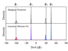
Figure 1: Demonstration of RJMCMC output. (top) Histogram of the posterior samples of the DoAs and (bottom) its Gaussian mixture approximation after relabeling. The data was generated from 4 sources with $\phi_{j}\in\{-60^{\circ},-15^{\circ},30^{\circ},45^{\circ}\}$ with a corresponding SNR of $\gamma_{j}\in\{-6\text{ dB},4\text{ dB},0\text{ dB},-4\text{ dB}\}$.

Estimation

Estimation can also be performed by inspecting the marginal density of the DoAs $\phi_{1},\ldots,\phi_{k}$ for any $k$, or the DoAs conditional on the output of the decision problem $\phi_{1},\ldots,\phi_{\widehat{k}}\mid\widehat{k}$. The former corresponds to performing Bayesian model averaging, while the latter corresponds to Bayesian model selection. This can be done using the same RJMCMC samples used for the detection problem. One issue when analyzing the DoAs through RJMCMC samples is that the individual DoA $\phi_{j}$ is subject to “label switching.” That is, for each posterior sample $\mathbfit{\theta}_{k}=(\mathbfit{\phi}_{1\text{:}k},\mathbfit{\gamma}_{1\text{:}k})$, there is no way to know to which source the DoAs $\phi_{1},\ldots,\phi_{k}$ belong to. Therefore, to analyze the parameters of a specific source, it is necessary to relabel each DoA $\phi_{j}$ and its local variable $\gamma_{j}$.

For relabeling, we use the mixture model fitting procedure proposed by Roodaki et al. [70]. This procedure assumes that the $k$ DoAs $\mathbfit{\phi}_{1\text{:}k}=(\phi_{1},\ldots,\phi_{k})$ in $\mathbfit{\theta}_{k}$ are sampled without replacement from a mixture of $\kappa\in\mathbb{N}_{>0}$ Gaussian components and a uniform component representing outliers. For $\kappa$, we choose the 90% percentile of the posterior of $k$, as proposed in [70]. An example is demonstrated in Fig. 1: In contrast to the “unlabeled” posterior (gray), the components of the mixture approximation (colored) can readily be used to quantify the uncertainty or obtain point estimates of the individual sources.

Reconstruction

The latent source signals can be reconstructed through the following sampling procedure:

$$k,\mathbfit{\phi}_{1\text{:}k},\mathbfit{\gamma}_{1\text{:}k} \sim\pi\left(k,\mathbfit{\phi}_{1\text{:}k},\mathbfit{\gamma}_{1\text{:}k}\mid\mathbfit{y},\alpha,\beta,\alpha_{\lambda},\alpha_{\beta}\right)$$ (20)

$$\mathbfit{x}_{1\text{:}k} \sim p\left(\mathbfit{x}_{1\text{:}k}\mid\mathbfit{y},k,\mathbfit{\phi}_{1\text{:}k},\mathbfit{\gamma}_{1\text{:}k}\right).$$ (21)

That is, for each RJMCMC sample, the closed-form conditional in Eq. 17 can be used to sample from the latent source signal posterior. The “labels” generated by the relabeling procedure of Roodaki et al. [70] can be used to register the source signal samples to their corresponding source.

IV-B Computing the Likelihood in the Frequency Domain

The collapsed likelihood in Eq. 16 involves matrix operations that are quite costly. For instance, naively computing $\mathbfit{P}_{\bot}$ has a complexity of $\mathcal{O}(N^{3}k^{3})$. We will now discuss how to improve this by leveraging the frequency domain representation of FIR filters.

Stripe Decomposition

The matrix representation of an FIR filter with periodic coefficients exhibits a structure known as a circulant matrix [49, §3]. Furthermore, a circulant matrix such as $\mathbfit{H}_{i,j}$ admits a spectral decomposition

$$\mathbfit{H}_{i,j}=\mathbfit{W}\mathbfit{S}_{i,j}\mathbfit{W}^{\dagger},$$ (22)

where $\mathbfit{S}_{i,j}$ is the spectrum of $h^{\prime}_{i,j}$, and $\mathbfit{W}^{\dagger},\mathbfit{W}\in\mathbb{C}^{N^{\prime}\times N^{\prime}}$ are the normalized $N^{\prime}$-point DFT matrix and its inverse. Recall that our choice of filter has a closed form DFT provided in [46]. Therefore, we can directly compute $\mathbfit{S}_{i,j}$ from $\phi_{j}$. From these facts, the concatenation $\mathbfit{H}\triangleq\mathbfit{H}_{1\text{:}M,1\text{:}k}$ admits a matrix decomposition we call a stripe decomposition through Proposition 1 in Appendix A. That is, there exists a matrix $\mathbfit{S}\in\mathbb{C}^{MN^{\prime}\times kN^{\prime}}$ such that

$$\mathbfit{H}=\mathbfit{\Phi}_{M}\,\mathbfit{S}\,\mathbfit{\Phi}_{k}^{\dagger},$$ (23)

where $\mathbfit{\Phi}_{M}^{\dagger}\in\mathbb{C}^{MN^{\prime}\times MN^{\prime}}$ is a block-wise DFT defined as

$$\mathbfit{\Phi}_{M}^{\dagger}\triangleq\mathrm{block\text{-}diagonal}_{M}\left(\mathbfit{W}^{\dagger},\ldots,\mathbfit{W}^{\dagger}\right),$$ (24)

is a unitary matrix, $\mathbfit{S}$ is a stripe matrix such that each $i,j$th block for $(i,j)\in[M]\times[k]$ is a diagonal matrix

$${[\mathbfit{S}]}_{i,j}\triangleq\mathbfit{S}_{i,j}=\mathrm{diagonal}\left(s_{i,j}[0],\ldots,s_{i,j}[N^{\prime}\text{-}1]\right),$$

where $s_{i,j}[0],\ldots,s_{i,j}[N^{\prime}-1]$ are the DFT coefficients of $h_{i,j}^{\prime}$. Again, for our choice of time delay filter (Section III-A), these have a closed form given $\phi_{j}$ [46]. Crucially, $\mathbfit{S}$ is not a diagonal matrix nor a block diagonal matrix, but a sparse structure referred to as (diagonally) striped by Smolarski [71]. We will refer to such structured matrix as a stripe matrix.

Similarly, our source signal covariance $\mathbfit{\Sigma}\triangleq\mathbfit{\Sigma}\left(\mathbfit{\gamma}_{1\text{:}k}\right)$ also admits a stripe decomposition

$$\mathbfit{\Sigma}=\mathbfit{\Phi}_{k}\mathbfit{T}\,\mathbfit{\Phi}_{k}^{\dagger},$$ (25)

where the stripe matrix $\mathbfit{T}\in\mathbb{R}^{kN^{\prime}\times kN^{\prime}}$ is symmetric block-diagonal where each $j$th block for $j\in[k]$ is given as

$${[\mathbfit{T}]}_{j,j}=\gamma_{j}\,\mathbf{I}_{N^{\prime}}.$$ (26)

We also point out that $\mathbfit{T}$ is positive definite (PD).

Stripe-decomposable matrices can be transposed, added, and multiplied efficiently in the space of stripe matrices. Furthermore, their inverse and determinant also directly follow from the inverse and determinant of the corresponding stripe matrix. (See Proposition 2 in Appendix A).

Approximate Collapsed Likelihood

Given Eq. 23, we can now represent the full system matrix using stripe matrices. That is,

$$\mathbfit{A}=\mathbfit{M}_{M}\,\mathbfit{\Phi}_{M}\mathbfit{S}\,\mathbfit{\Phi}_{k}^{\dagger}$$ (27)

Unfortunately, the truncation operation $\mathbfit{M}$ complicates computation as it does not admit a stripe decomposition. This is because truncation cannot be represented as an LTI system. Therefore, we further rely on the approximation

$$\mathbfit{M}_{M}^{\top}\mathbfit{M}_{M}\approx\mathbf{I}_{MN^{\prime}}.$$ (28)

Remark 1.

The basic consequence of the approximation in Eq. 28 is that the system does not ignore the zero padding in $\mathbfit{y}_{\mathcal{F}}$. Therefore, the non-causal part of the latent source signal will revert towards zero with high confidence.

Now, the collapsed likelihood is approximately given as

$$\text{\lx@cref{creftype~refnum}{eq:collapsed_likelihood}}\approx{\left(\mathrm{det}\left(\mathbfit{T}^{-1}\right)/\mathrm{det}\left(\mathbfit{T}^{-1}+\mathbfit{S}^{\dagger}\,\mathbfit{S}\right)\right)}^{\nicefrac{{1}}{{2}}}$$

$$\;\times{\left(\frac{\alpha}{2}+\mathbfit{y}^{\dagger}\mathbfit{y}-\mathbfit{y}_{\mathcal{F}}^{\dagger}\,\mathbfit{S}\,{\left(\mathbfit{T}^{-1}+\,\mathbfit{S}^{\dagger}\mathbfit{S}\right)}^{-1}\mathbfit{S}^{\dagger}\mathbfit{y}_{\mathcal{F}}\right)}^{-\nicefrac{{MN}}{{2}}+\beta},$$ (29)

where $\mathbfit{y}_{\mathcal{F}}\triangleq\mathbfit{\Phi}_{M}^{\dagger}\mathbfit{M}^{\top}_{M}\mathbfit{y}\in\mathbb{C}^{MN^{\prime}}$ is the padded blockwise-normalized-DFT of $\mathbfit{y}$. The full derivation of Eq. 29 is given in Appendix B.

Input: Stripe matrix $\mathbfit{R}\in\mathbb{C}^{kN^{\prime}\times kN^{\prime}}$ with $N^{\prime}\times N^{\prime}$ blocks.

for  $i=1,\ldots,k$  do

       $\mathbfit{D}_{ii}=\mathbfit{R}_{ii}-{\textstyle\sum^{j-1}_{k=1}}\mathbfit{L}_{jk}\mathbfit{D}_{kk}\mathbfit{L}_{jk}^{*}$

       for  $j=1,\ldots,k$  do

            

$$\mathbfit{L}_{ij} =\begin{cases}\;\;1&\;\text{if $i=j$}\\ \;\;\left(\mathbfit{R}_{ij}-{\textstyle\sum^{j-1}_{k=1}}\mathbfit{L}_{ik}\mathbfit{D}_{kk}\mathbfit{L}_{jk}^{*}\right)\,\mathbfit{D}_{ii}^{-1}&\;\text{if $i>j$}\\ \;\;0&\;\text{otherwise}\end{cases}$$

       end for

      

end for

Algorithm 1 Block-LDL^⊤ Decomposition

Computation with the LDL^⊤ Decomposition

Let

$$\mathbfit{R}\triangleq\mathbfit{T}^{-1}+\mathbfit{S}^{\dagger}\mathbfit{S}\qquad\text{and}\qquad\mathbfit{z}\triangleq\mathbfit{S}^{\dagger}\mathbfit{y}_{\mathcal{F}}$$ (30)

for clarity. Eq. 29 requires computing the determinant $\det\left(\mathbfit{R}\right)$ and quadratic form $\mathbfit{z}^{\dagger}\mathbfit{R}^{-1}\mathbfit{z}$, which is not trivial even with stripe matrices. For this, Ladaycia et al. [72] proposed to use the Schur complement recursively, which, for $\mathbfit{R}\in\mathbb{C}^{kN^{\prime}\times kN^{\prime}}$ comprised of $N^{\prime}\times N^{\prime}$ blocks, yields its inverse $\mathbfit{R}^{-1}$ and determinant $\det\mathbfit{R}$ in $\mathcal{O}\left(k^{3}N\right)$ time. Unfortunately, the recursive Schur complement is numerically unstable. Instead, since $\mathbfit{R}$ is always PD as $\mathbfit{T}$ is PD, we can consider decompositions specialized for PD matrices such as the Cholesky or LDL^⊤ decompositions. In our case, we observed that LDL^⊤ was numerically more stable. For a PD matrix such as $\mathbfit{R}$, the LDL^⊤ decomposition yields the unique lower triangular matrix $\mathbfit{L}\in\mathbb{C}^{kN^{\prime}\times kN^{\prime}}$ and diagonal matrix $\mathbfit{D}\in\mathbb{C}^{kN^{\prime}\times kN^{\prime}}$ such that

$$\mathbfit{R}=\mathbfit{L}\mathbfit{D}\mathbfit{L}^{\dagger}.$$ (31)

Conveniently, for stripe matrices, computing the block-LDL^⊤ decomposition [73, Algorithm 4.1], shown in Algorithm 1, yields the full LDL^⊤ decomposition (Proposition 3 in Appendix A), where $\mathbfit{L}$ has the same stripe matrix structure as $\mathbfit{R}$ in the lower triangular region. This takes $\mathcal{O}(k^{3}N)$ operations.

Equipped with the LDL^⊤ decomposition of $\mathbfit{R}$, we can now compute the quadratic form and determinants as

$$\mathbfit{z}^{\dagger}\mathbfit{R}^{-1}\mathbfit{z}={\left\lVert\mathbfit{L}^{-1}\mathbfit{z}\right\rVert}_{\mathbfit{D}^{-1}}^{2}\;\;\text{and}\;\;\mathrm{det}\left(\mathbfit{R}\right)={\textstyle\prod^{k}_{j=1}}\det\left(\mathbfit{D}_{jj}\right).$$ (32)

Similarly to Algorithm 1, $\mathbfit{L}^{-1}\mathbfit{z}$ can be computed through a block forward-substitution and the determinant of a diagonal matrix such as $\mathbfit{D}_{jj}$ is the product of the diagonal. This now completes computing Eq. 29. Whenever the LDL^⊤ decomposition fails, or the resulting likelihood is not strictly positive due to numerical errors, we set the likelihood as $0$ such that RJMCMC can reject the offending proposal.

Computational Complexity

The main bottleneck of computing Eq. 29 is computing the LDL^⊤ decomposition, which takes $\mathcal{O}(Nk^{3})$ operations. The forward substitution also takes $\mathcal{O}(Nk^{2})$ operations. Since $\mathbfit{y}_{\mathcal{F}}$ only needs to be computed once, the cost of the DFT is fully amortized. The products $\mathbfit{S}^{\dagger}\mathbfit{S}$ and $\mathbfit{S}^{\dagger}\mathbfit{y}_{\mathcal{F}}$ take $\mathcal{O}(k^{3}N)$ and $\mathcal{O}(NMk)$ operations, respectively. Therefore, the overall cost is $\mathcal{O}(Nk^{3}+NMk)$. Note that, $k\leq k_{\text{max}}<M$. Therefore, the worst-case complexity can be summarized to $\mathcal{O}(NM^{3})$. This is comparable to the cost of computing the likelihood of time-frequency models [1, Eq. 14.99, Eq. 14.102], which is $\mathcal{O}(BM^{2}k)$, where the pseudoinverse of the $M\times k$ “steering matrix” is computed for each of the $B$ frequency bins.

IV-C Inference with Non-Reversible Jump MCMC

Now, we will discuss how to draw samples from the posterior in Eq. 18. Let us denote a single collection of parameters for a sample as $\mathbfit{\theta}_{k}=\left(\mathbfit{\phi}_{1\text{:}k},\mathbfit{\gamma}_{1\text{:}k}\right)\in\mathbb{R}^{d_{k}}$ such that the target posterior is also denoted $\pi\left(k,\mathbfit{\theta}_{k}\right):\cup_{k\in\mathcal{K}}\{k\}\times\mathbb{R}^{d_{k}}\to\mathbb{R}_{\geq 0}$, where $\mathcal{K}=[k_{\mathrm{max}}]$. Unlike typical Bayesian analysis setups, the dimension of our posterior changes depending on $k$. Reversible jump Markov chain Monte Carlo (RJMCMC; [33, 35, 34, 36]) is a family of MCMC algorithms [66] specialized for such setting. In particular, we use the birth-death-update process [33] with its non-reversible extension proposed by Gagnon and Doucet [47].

Reversible Jump MCMC

Traditional RJMCMC [33] operates analogously to Metropolis-Hastings [74, 75], where, given a state of the Markov chain $(k,\mathbfit{\theta}_{k})$, a transition to a different model space $k^{\prime}$ may be proposed as

$$k^{\prime}\sim q\left(k,k^{\prime}\right).$$ (33)

When $k\neq k^{\prime}$, the proposal “jumps” to a different model space $k^{\prime}$. Therefore, such a proposal is referred to as a jump proposal and $q\left(k,k^{\prime}\right)$ is referred to a jump proposal kernel. The parameters in the model space of $k^{\prime}$ of the jump proposal are $\mathbfit{\theta}^{\prime}$ computed as

$$\left(\mathbfit{\theta}_{k^{\prime}},\mathbfit{u}_{k^{\prime}\mapsto k}\right)=\mathcal{T}_{k\mapsto k^{\prime}}\left(\mathbfit{\theta}_{k},\mathbfit{u}_{k\mapsto k^{\prime}}\right),$$ (34)

where $\mathbfit{u}_{k\mapsto k^{\prime}}$ are the auxiliary variables needed to enable the jump, which are sampled as

$$\mathbfit{u}_{k\mapsto k^{\prime}}\sim q_{k\mapsto k^{\prime}}\left(\mathbfit{u}_{k\mapsto k^{\prime}}\right).$$ (35)

The proposal $(k^{\prime},\mathbfit{\theta}_{k^{\prime}})$ is then accepted or rejected according to a Metropolis-Hastings step (MH) with probability

$$\alpha\left(\left(k^{\prime},\mathbfit{\theta}_{k^{\prime}}\right),\left(k,\mathbfit{\theta}_{k}\right)\right)=\min\left(1,r\right)$$ (36)

according to the Metropolis-Hastings-Green (MHG) ratio

$$r=\frac{\pi\left(k^{\prime},\mathbfit{\theta}_{k^{\prime}}\right)}{\pi\left(k,\mathbfit{\theta}_{k}\right)}\frac{q\left(k^{\prime},k\right)}{q\left(k,k^{\prime}\right)}\frac{q_{k^{\prime}\mapsto k}\left(\mathbfit{u}_{k^{\prime}\mapsto k}\right)}{q_{k\mapsto k^{\prime}}\left(\mathbfit{u}_{k\mapsto k^{\prime}}\right)}{J_{k\mapsto k^{\prime}}\left(\mathbfit{\theta}_{k},\mathbfit{u}_{k\mapsto k^{\prime}}\right)},$$

where $J_{k\mapsto k^{\prime}}$ denotes the absolute determinant of the Jacobian of $\mathcal{T}_{k\mapsto k^{\prime}}$. Since we use the birth-death-update process, which only adds or removes elements, $J_{k\mapsto k^{\prime}}=1$.

Input: update move probability $\tau\in(0,1)$.

$u\sim\mathsf{Uniform}\left[0,1\right]$

if $u<\tau$ then

       Execute update move

else

       $k^{\prime}=k+v$

       $\mathbfit{u}_{k\mapsto k^{\prime}}\sim q_{k\mapsto k^{\prime}}\left(\mathbfit{u}_{k\mapsto k^{\prime}}\right)$

       $\left(\mathbfit{\theta}_{k^{\prime}},\mathbfit{u}_{k^{\prime}\mapsto k}\right)\leftarrow\mathcal{T}_{k\mapsto k^{\prime}}\left(\mathbfit{\theta}_{k},\mathbfit{u}_{k\mapsto k^{\prime}}\right)$

       Compute $\alpha\leftarrow\min(1,r)$ with $r$ in Eq. 37

       Accept or reject $(k^{\prime},\mathbfit{\theta}_{k^{\prime}})$ with probability $\alpha$

       if  rejected  then

             $v\leftarrow-v$

            

       end if

      

end if

Algorithm 2 Non-Reversible Jump MCMC Transition

Non-Reversible Jump MCMC

Over the years, it has been shown that simulating non-reversible processes often result in faster mixing and lower autocorrelation [76]. For the RJMCMC setting, Gagnon and Doucet [47] proposed to apply a technique known as lifting, which augments the Markov chain with a binary random variable $v\in\{+1,-1\}$ such that the Markov chain is now ${\{(k^{t},\mathbfit{\theta}_{k^{t}}^{t},v^{t}))\}}_{t\geq 0}$. In the context of RJMCMC, at each MCMC step, the jump proposal is now deterministically chosen as $k^{\prime}=k+v$, and we proceed with the MH step with the ratio

$$r=\frac{\pi\left(k^{\prime},\mathbfit{\theta}_{k^{\prime}}\right)}{\pi\left(k,\mathbfit{\theta}_{k}\right)}\frac{q_{k^{\prime}\mapsto k}\left(\mathbfit{u}_{k^{\prime}\mapsto k}\right)}{q_{k\mapsto k^{\prime}}\left(\mathbfit{u}_{k\mapsto k^{\prime}}\right)}J_{k\mapsto k^{\prime}}\left(\mathbfit{\theta}_{k},\mathbfit{u}_{k\mapsto k^{\prime}}\right).$$ (37)

The “jump direction” $v$ is flipped whenever the proposal is rejected. The resulting chain is now a piecewise-deterministic Markov process (PDMP), which is non-reversible but preserves the correct stationary distribution and often results in lower autocorrelation both empirically [47] and theoretically [77]. The non-reversible jump MCMC (NRJMCMC) algorithm is described in detail in Algorithm 2.

Birth-Death-Update Process

For the jump moves, we use the classic birth-death-update process [33]. It alternates between the birth, death, and update moves, which correspond to the jump move proposed when $k^{\prime}=k+1$, $k^{\prime}=k-1$, and $k^{\prime}=k$ respectively. The birth move increases the model order through insertion:

$$\mathbfit{\phi}_{1\text{:}k}\oplus_{j}\phi^{\prime}=\left(\phi_{1},\ldots,\phi_{j-1},\phi^{\prime},\phi_{j},\ldots,\phi_{k}\right),$$ (38)

while the death move decreases the model order through removal

$$\mathbfit{\phi}_{1\text{:}k,-j}=\left(\phi_{1},\ldots,\phi_{j-1},\phi_{j+1},\ldots,\phi_{k}\right),$$ (39)

and the update move updates the parameters through a regular MCMC kernel without altering the model order.

Birth Move

During the birth move, a newborn $(\phi^{\prime},\gamma^{\prime})$ and its insertion position $j$ are proposed as

$$\phi^{\prime}\sim q\left(\phi\right),\quad\gamma^{\prime}\sim q\left(\gamma\right),\quad j\sim\mathsf{Uniform}\left\{0,\ldots,k\right\},$$

forming the auxiliary variable $\mathbfit{u}_{k\mapsto k+1}=\left(\phi^{\prime},\gamma^{\prime},j\right)$.

The birth proposal is then

$$\mathbfit{\theta}_{k+1}=\left(\mathbfit{\phi}_{1\text{:}k}\oplus_{j}\phi^{\prime},\;\;\mathbfit{\gamma}_{1\text{:}k}\oplus_{j}\gamma^{\prime}\right)=\mathcal{T}_{k\mapsto k+1}\left(\mathbfit{\theta}_{k},\mathbfit{u}_{k\mapsto k+1}\right).$$

The probability densities of the auxiliary variables for the forward and backward jumps of the birth move are given as

$$q_{k\mapsto k+1}\left(\mathbfit{u}_{k\mapsto k+1}\right) =\frac{1}{k+1}q\left(\phi^{\prime},\gamma^{\prime}\right),$$ (Birth Forward)

$$q_{k+1\mapsto k}\left(\mathbfit{u}_{k+1\mapsto k}\right) =\frac{1}{k+1}.$$ (Birth Reverse)

Previously, a common practice following [37] was to insert the newborn at the end of the vector. As demonstrated by Roodaki et al. [78], this breaks the symmetry between the birth and death moves, resulting in a biased RJMCMC procedure, hence the involvement of $j$ here.

Death Move

For the death move, we only have to select the index of the removal candidate

$$j\sim\mathsf{Uniform}\left\{1,\ldots,k\right\},$$ (40)

where it is then removed as

$$\mathbfit{\theta}_{k-1}=\left(\mathbfit{\phi}_{1\text{:}k,-j},\;\;\mathbfit{\gamma}_{1\text{:}k,-j}\right)=\mathcal{T}_{k\mapsto k-1}\left(\mathbfit{\theta}_{k},\mathbfit{u}_{k\mapsto k-1}\right).$$

The auxiliary variable is then $\mathbfit{u}_{k\mapsto k-1}=j$. The densities for the forward and backward auxiliary variables are given as

$$q_{k\mapsto k-1}\left(\mathbfit{u}_{k\mapsto k-1}\right) =\frac{1}{k},$$ (Death Forward)

$$q_{k-1\mapsto k}\left(\mathbfit{u}_{k-1\mapsto k}\right) =\frac{1}{k}q\left(\phi_{j},\gamma_{j}\right). \quad\text{(Death Reverse)}.$$

Update Move

For the update move, we apply the slice sampling algorithm by Neal [79]. Compared to independent or random-walk MH [75] used in previous works [44, 14, 38, 39, 40, 41, 42, 43], it achieves remarkable performance both in practice and in theory. (See [80] and references therein.) Furthermore, the posterior of the DoAs is multimodal, making gradient-based samplers ineffective. In contrast, we observe that slice sampling handles multimodality well, as long as the “search interval” is chosen to be wide enough. In this work, we use the “stepping-out” variant [79, Scheme 3] with an initial search interval of $w=2$, which is augmented into a coordinate-wise Gibbs scheme [81, 82] with random permutation scans [66, Alg. 42]. The update move selection probability is set as $\tau=0.1$.

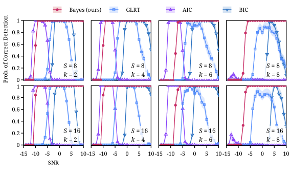
Figure 2: Wideband signal detection performance versus SNR, # of snapshots ($S$), and # of targets ($k$). The solid lines are the mean estimated from 100 replications, while the colored bands are $95\%$ bootstrap confidence intervals of the mean.

V Evaluation

V-A Experimental Setup

Implementation

We implemented our proposed scheme in the Julia language [83]. The probability distributions were provided by the Distributions.jl library [84] and the stripe matrix operations were implemented using the Tullio.jl [85] array programming framework. The correctness of our RJMCMC implementation was verified through the tests proposed by Gandy and Scott [86]. For the auxiliary jump variable proposal, we use the following generic choice:

$$q\left(\phi\right)=\mathsf{Uniform}\left(\phi;\left[-\nicefrac{{\pi}}{{2}},\nicefrac{{\pi}}{{2}}\right]\right);\;\;q\left(\gamma\right)=\mathsf{LogNormal}\left(\gamma;0,2\right).$$

To ensure $\gamma_{j}$ stays within $\mathbb{R}_{>0}$, we sample it in log space and apply a Jacobian adjustment to the joint likelihood. For the remaining hyperparameters, we set $\alpha=\beta=0$, which yields Jeffrey’s scale prior [57]. The maximum number of targets is $k_{\max}=M-1$. For the detection experiments, we draw $2^{12}$ posterior samples with NRJMCMC after discarding $2^{10}$ samples as burn-in and apply the procedure in Section IV-A.

All of the code used in this work is publicly available. Under our current implementation, for $k=4$ targets, $M=20$ sensors, and a received signal with $N=256$ samples, drawing $2^{12}$ RJMCMC samples takes roughly 18 seconds on a Dell XPS15 9520 laptop equipped with an Intel i7-12700H CPU.

Baselines

We consider the following baselines:

• GLRT: This is a GLRT-based detection method proposed by Chung et al. [23]. The $p$-values are obtained by bootstrapping [27] over the frequency bins, where multiple testing is performed according to the Benjamini-Hochberg procedure [87], which controls the false discovery rate $q\in(0,1)$. Following [23], we choose $q=0.1$.

• AIC, BIC: These are the classical information theoretic approaches as proposed by Akaike [88] using the AIC and BIC criteria, respectively [5, 6]. The BIC criterion was also commonly referred to as the minimum description length (MDL) criterion in the signal-processing literature.

Both approaches require solving a series of maximum likelihood problems over the range of models $k=1$ up to $k=k_{\mathrm{max}}$ We give a slight advantage to the baselines by narrowing down the range to $k_{\mathrm{max}}=10$ instead of $M-1$ as for RJMCMC. We use the likelihood of the deterministic signal model [1, §3.14.5.1.1, Eq. 14.99], which is maximized through the space alternating generalized expectation maximization (SAGE) algorithm [89] analyzed in [90]. (The general SAGE algorithm was originally proposed in [91].) To deal with multimodality, we initialize each linesearch with DIRECT [92] followed by refinement with L-BFGS [93].

Simulation Methodology

For each $j\in[k]$ for a true $k$, we generate $\mathbfit{x}_{j}$ by band-limiting white Gaussian noise to have a signal power of $P_{j}=\mathbb{E}\mathbfit{x}_{j}^{2}$. The signal is then delayed using the FIR delay filter by Pei and Lai [46]. Lastly, white Gaussian noise $\mathbfit{\eta}$ with power $\sigma^{2}$ is added over the channels as $\mathbfit{y}=\mathbfit{x}_{1\text{:}k}+\mathbfit{\eta}$, such that the $j$th source signal has an $\mathrm{SNR}=10\log_{10}P_{j}/\sigma^{2}$ [dB]. For ML-based methods that use the time-frequency model, the received signal $\mathbfit{y}$ is STFT-ed with $B=32$ frequency bins with a rectangular window and no overlap. Since we only use real-valued signals, a one-sided STFT is applied, resulting in 16 frequency bins after excluding the DC bin. The sampling frequency is $f_{s}=3$k Hz, the array is a ULA with 20 sensors, the sensor spacing is 0.5 m, and the propagation speed is $c=1500$ m/s.

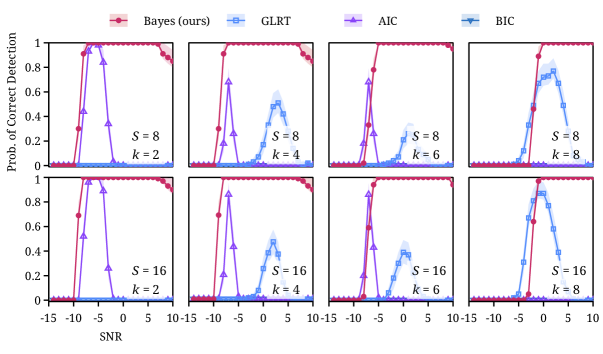
Figure 3: Narrowband signal detection performance versus SNR, # of snapshots ($S$), and # of targets ($k$). The solid lines are the mean estimated from 100 replications, while the colored bands are $95\%$ bootstrap confidence intervals of the mean.

V-B Wideband Signal Detection Performance

Setup

For the first experiment, we apply the considered detection methods on equally-spaced, equally-powered wideband signals with varying snapshots, targets, and SNR. For our Bayesian procedure (Bayes), which does not involve the STFT, we use the equivalent number of $N=B\cdot S$ samples. The bandwidths of the source signals were set to be [10 Hz, 1k Hz], which is slightly less than the half-wavelength constraint, making the problem more challenging.

Results

The results are shown in Fig. 2. AIC generally performs poorly due to the well-known issue of overestimating the number of sources. In contrast, GLRT and BIC maintain high accuracy for a wider range of SNRs, where GLRT is better in low SNRs, while BIC is better at high SNRs. Compared to these, our Bayesian detection procedure exhibits good low-SNR performance while maintaining high accuracy for the widest range of SNRs.

V-C Narrowband Signal Detection Performance

Setup

Next, we evaluate the performance of wideband detection methods faced with narrowband signals. Similarly to Section V-B, we consider equally-powered equally-spaced signals, where the bandwidth is set as [500 Hz, 600 Hz], which is close to a single frequency bin.

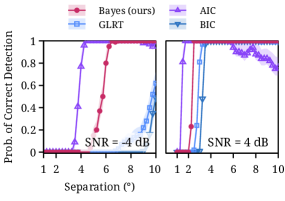
(a)

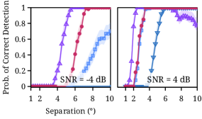
(b)

Figure 4: Detection performance versus angular separation and SNR. The solid lines are the mean estimated from 100 replications, while the colored bands are $95\%$ bootstrap confidence intervals of the mean.

Results

The results are shown in Fig. 3. For narrowband signals, information-theoretic methods perform much poorly. This is because the complexity penalty penalizes the complexity of modeling all the frequency bins, while the improvement in likelihood comes from only a single bin. In contrast, Bayes showed good performance for a wide range of SNR. However, unlike the wideband case, it required a higher SNR to transition to correctly detecting the targets. Meanwhile, GLRT underperformed compared to Bayes. While the performance of GLRT shown here is worse compared to the performance reported in [23], this is because, unlike in [23], we applied the wideband version of GLRT to a narrowband signal: the bins not containing the target signal reduce the overall power of the test procedure.

V-D Angular Resolution

Setup

We evaluate the effect of angular separation on the detection performance. We generate two equally powered signals and see how far the signals must be separated to correctly estimate the number of signals $k=2$. The experiments is performed for wideband (bandwidth of [10 Hz, 1k Hz]) and narrowband (bandwidth of [500 Hz, 600 Hz]) signals. We use $S=8$ snapshots in all cases.

Results

The results are shown in Fig. 4. Here, AIC is shown to be the most sensitive with respect to angular separation. From the results in Sections V-B and V-C, however, we have seen that this is at the cost of much worse performance in the high-SNR regime. Our Bayesian procedure comes out second, where the angular resolution at -4 dB is significantly better than BIC and GLRT. Clearly, the angular resolution of BIC and GLRT are significantly impacted by the SNRs, while Bayes is impacted much less.

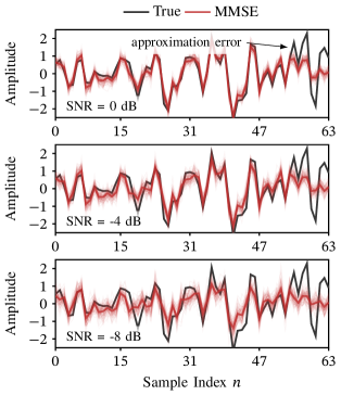
Figure 5: Reconstructions of a latent source signal. MMSE is the minimum mean-square error estimate, which is the posterior mean. The lightly shaded lines are 100 random samples from the posterior.

V-E Reconstruction

For the last experiment, we qualitatively evaluate the signal reconstruction performance. This is not only to evaluate the reconstruction capabilities of the proposed scheme but also to visually demonstrate the effect of the modeling assumptions imposed in Section III-B.

Setup

We generated a single wideband signal at $\phi=-\pi/4$ with bandwidth [10 Hz, 1k Hz] under varying SNRs. Then, we sampled $10^{3}$ MCMC samples (no jump moves) after $10^{3}$ burn-in steps. After that, the reconstruction procedure in Section IV-A was applied.

Results

The reconstructed signals are shown in Fig. 5. The signals are overall accurately reconstructed up to -4 dB, but are less accurate at -8 dB, which is the point where our methods started to break down as shown in the past experiments. Note the reconstruction past $n=50$ is inaccurate even at 0 dB. This is none other than the non-causal part of the signal. Due to the approximation in Eq. 28, the signal reverts to 0 with high confidence as mentioned in Remark 1. Without the approximation Eq. 28, the signals would have still reverted to 0, as it is the prior mean, but the uncertainty (posterior variance) would have increased. The negative impact of this misspecification can be seen in Fig. 3, where the accuracy starts to decrease at very high SNRs.

VI Discussions

In this work, we have exploited the full strength of the Bayesian framework for wideband signal processing: signal detection, DoA estimation, and signal reconstruction can all be done from a single probabilistic model. On the signal detection problem, our Bayesian approach outperformed frequentist and information-theoretic approaches. We also described techniques to accelerate the computation of our model, making the computation cost comparable to alternatives.

Limitations

The main limitation of our approach is the use of the approximation in Eq. 28. While this is necessary to keep all computations in the frequency domain, it leads to underestimation of the uncertainty of the non-causal part of the latent signal. As such, our model ends up being misspecified even for the synthetic data we used in Section V. In model comparison terms, we are operating in the “$\mathcal{M}$-completed” regime [94]: the model is misspecified, but comparing model posterior probabilities is still useful. Indeed, our approach showed good performance in Section V. However, the effect of misspecification can be noticed in Fig. 3 in the high SNR regime. Avoiding Eq. 28 while maintaining computational tractability would lead to a more powerful detection scheme in the high SNR-low snapshot regime.

Future Directions

The strength of the Bayesian paradigm is that it is easy to encode prior knowledge and assumptions into the model. Therefore, an immediate future direction is to investigate other signal priors as mentioned at the end of Section III-B or extend our model to incorporate colored noise [14], non-Gaussian noise, and non-uniform arrays. However, no matter how much modeling we do, any model will be misspecified when faced with real data. Therefore, investigating the benefit of Bayesian modeling comparison procedures targeting the “$\mathcal{M}$-open” regime [94] (e.g., [95, 96]), where traditional Bayesian model comparison breaks down, would be important. Lastly, the estimation performance of our proposed method is of independent interest, where evaluation against procedures specialized to DoA estimation such as those in [22, 19, 97, 98], and Cramer-Rao lower bounds as in [44], could be useful.

Appendix A Stripe-Decomposable Matrices

We discuss the definition and properties of stripe-decomposable matrices.

Definition 1.

We say a matrix $\mathbfit{A}\in\mathbb{C}^{ML\times NL}$ is stripe decomposable with $L\times L$ blocks if there exist a decomposition

$$\mathbfit{A}=\mathbfit{\Phi}_{M}\,\mathbfit{S}\,\mathbfit{\Phi}_{N}^{\dagger},$$

where, for any $K\in\mathbb{N}_{>0}$, $\mathbfit{\Phi}_{K}\in\mathbb{C}^{KL\times KL}$ is some unitary matrix such that $\mathbfit{\Phi}_{K}\mathbfit{\Phi}_{K}^{\dagger}=\mathbf{I}_{KL}$, and the corresponding “stripe matrix” $\mathbfit{S}\in\mathbb{C}^{ML\times NL}$ is structured as

$$\mathbfit{S}=\begin{bmatrix}\mathbfit{S}_{1,1}&\ldots&\mathbfit{S}_{1,N}\\ \vdots&\ddots&\vdots\\ \mathbfit{S}_{M,1}&\ldots&\mathbfit{S}_{M,N}\\ \end{bmatrix},$$

where $\mathbfit{S}_{i,j}\in\mathbb{C}^{L\times L}$ for $(i,j)\in[M]\times[N]$ is a diagonal matrix.

Proposition 1.

Let $\mathbfit{A}\in\mathbb{C}^{ML\times NL}$ be a block-structured matrix such that

$$\mathbfit{A}=\begin{bmatrix}\mathbfit{A}_{1,1}&\ldots&\mathbfit{A}_{1,L}\\ \vdots&\ddots&\vdots\\ \mathbfit{A}_{M,1}&\ldots&\mathbfit{A}_{M,L}\\ \end{bmatrix},$$

where each block $\mathbfit{A}_{i,j}\in\mathbb{R}^{L\times L}$ admits a spectral decomposition $\mathbfit{A}_{i,j}=\mathbfit{P}\mathbfit{D}_{i,j}\mathbfit{P}^{\dagger}$ for $(i,j)\in[M]\times[N]$ with the same unitary basis matrix $\mathbfit{P}$. Then, $\mathbfit{A}$ admits a stripe decomposition where the corresponding stripe matrix $\mathbfit{S}$ structured such that ${[\mathbfit{S}]}_{i,j}=\mathbfit{D}_{i,j}$ and $\mathbfit{\Phi}_{M}=\mathrm{block\text{-}diagonal}_{M}\left(\mathbfit{P},\ldots,\mathbfit{P}\right)$ and $\mathbfit{\Phi}_{N}=\mathrm{block\text{-}diagonal}_{N}\left(\mathbfit{P},\ldots,\mathbfit{P}\right)$.

Proof.

It suffices to check that

$${\left[\mathbfit{\Phi}_{M}\,\mathbfit{S}\,\mathbfit{\Phi}_{N}^{\dagger}\right]}_{i,j} =\sum_{k=1}^{M}\sum_{l=1}^{N}{\left[\mathbfit{\Phi}_{M}\right]}_{i,k}{\left[\mathbfit{S}\right]}_{k,l}{\left[\mathbfit{\Phi}_{M}^{\dagger}\right]}_{l,j}$$

$$=\sum_{k=1}^{M}\sum_{l=1}^{N}\mathbb{1}_{i=k}\mathbb{1}_{l=j}{\left[\mathbfit{\Phi}_{M}\right]}_{i,k}{\left[\mathbfit{S}\right]}_{k,l}{\left[\mathbfit{\Phi}_{M}^{\dagger}\right]}_{l,j}$$ (41)

$$={\left[\mathbfit{\Phi}_{M}\right]}_{i,i}{\left[\mathbfit{S}\right]}_{i,j}{\left[\mathbfit{\Phi}_{M}^{\dagger}\right]}_{j,j}$$

$$=\mathbfit{P}\,\mathbfit{D}_{i,j}\,\mathbfit{P}^{\dagger}$$

$$=\mathbfit{A}_{i,j}.$$

Eq. 41 is due to $\mathbfit{\Phi}_{M}$ and $\mathbfit{\Phi}_{N}$ being block-diagonal. ∎

Proposition 2.

Let $\mathbfit{A}=\mathbfit{\Phi}_{M}\,\mathbfit{S}\,\mathbfit{\Phi}_{N}^{\dagger}\in\mathbb{C}^{ML\times NL}$, $\mathbfit{B}=\mathbfit{\Phi}_{M}\,\mathbfit{T}\,\mathbfit{\Phi}_{N}^{\dagger}\in\mathbb{C}^{ML\times NL}$, $\mathbfit{C}=\mathbfit{\Phi}_{N}\,\mathbfit{U}\,\mathbfit{\Phi}_{K}^{\dagger}\in\mathbb{C}^{NL\times KL}$, and $\mathbfit{D}=\mathbfit{\Phi}_{M}\mathbfit{V}\mathbfit{\Phi}_{M}^{\dagger}\in\mathbb{C}^{ML\times ML}$, be stripe-decomposable matrices with $L\times L$ blocks, where $\mathbfit{D}$ is further assumed to be invertible. Then, the following properties hold:

$$\bullet \mathbfit{A}^{\dagger} =\,\mathbfit{\Phi}_{N}\,\mathbfit{S}^{\dagger}\,\mathbfit{\Phi}_{M}^{\dagger}$$ Hermitian Transpose:

$$\bullet \mathbfit{A}+\mathbfit{B} =\,\mathbfit{\Phi}_{M}\,\left(\mathbfit{S}+\mathbfit{T}\right)\,\mathbfit{\Phi}_{N}^{\dagger}$$ Addition:

$$\bullet \mathbfit{B}\,\mathbfit{C} =\,\mathbfit{\Phi}_{M}\,\mathbfit{T}\,\mathbfit{U}\,\mathbfit{\Phi}_{K}^{\dagger}$$ Multiplication:

$$\bullet \det\mathbfit{D} =\det\mathbfit{V}$$ Determinant:

$$\bullet \mathbfit{D}^{-1} =\,\mathbfit{\Phi}_{M}\,\mathbfit{V}^{-1}\,\mathbfit{\Phi}_{M}^{\dagger}.$$ Inverse:

Proof.

The transpose, addition, and multiplication relations are trivial.

Proof of Determinant

From the properties of the determinant, we have $\det\mathbfit{D}=\det\mathbfit{\Phi}_{M}\det\mathbfit{V}\det\mathbfit{\Phi}_{M}^{\dagger}=\det\mathbfit{V}$, where the last equality follows from the fact that $\mathbfit{\Phi}_{M}^{-1}=\mathbfit{\Phi}^{\dagger}_{M}$.

Proof of Inverse

Since $\mathbfit{D}$ is invertible, the matrix $\mathbfit{D}^{-1}$ such that $\mathbfit{D}\mathbfit{D}^{-1}=\mathbf{I}_{NL}$ exists and is unique. Also, from the fact that $\det\mathbfit{D}=\det\mathbfit{V}\neq 0$ it is evident that $\mathbfit{V}$ is invertible such that $\mathbfit{V}^{-1}$ uniquely exists. Now let $\mathbfit{E}\triangleq\mathbfit{\Phi}_{M}\mathbfit{V}^{-1}\mathbfit{\Phi}_{M}^{\dagger}$. It follows that

$$\mathbfit{D}\mathbfit{E} =\left(\mathbfit{\Phi}_{M}\mathbfit{V}\mathbfit{\Phi}_{M}^{\dagger}\right)\left(\mathbfit{\Phi}_{M}\mathbfit{V}^{-1}\mathbfit{\Phi}_{M}^{\dagger}\right)$$

$$=\mathbfit{\Phi}_{M}\mathbfit{V}\mathbfit{V}^{-1}\mathbfit{\Phi}_{M}^{\dagger}$$

$$=\mathbfit{\Phi}_{M}\mathbfit{\Phi}_{M}^{\dagger}$$

$$=\mathbf{I}_{ML}.$$

Therefore, it is clear that $\mathbfit{D}^{-1}=\mathbfit{E}$.

∎

Proposition 3.

Let $\mathbfit{S}\in\mathbb{C}^{NL\times NL}$ be a positive definite stripe matrix with $L\times L$ diagonal blocks. Applying Algorithm 1 to $\mathbfit{S}$ yields the block-LDL^⊤ decomposition

$$\mathbfit{S}=\mathbfit{L}\mathbfit{D}\mathbfit{L}^{\dagger}.$$

This is also the unique LDL^⊤ decomposition of $\mathbfit{S}$.

Proof.

Since $\mathbfit{S}$ is positive definite, its LDL^⊤ decomposition is unique. Now, since all the blocks of $\mathbfit{S}$ are diagonal matrices and $\mathbfit{L}$ has the same structure for the block-lower-triangular region, its upper-triangular, excluding the diagonal, is full of zeros. Therefore, $\mathbfit{L}$ is already a lower-triangular matrix and similarly, $\mathbfit{D}$ is already a diagonal matrix. Therefore, $\mathbfit{L}\mathbfit{D}\mathbfit{L}^{\dagger}$ is coincidentally the unique LDL^⊤ decomposition of $\mathbfit{S}$. ∎

Appendix B Derivation of Eq. 29

Recall that Eq. 16 is comprised as follows:

$${\underbrace{\mathrm{det}\left(\mathbfit{P}_{\bot}\right)}_{T_{\text{det}}}}^{-\nicefrac{{1}}{{2}}}{\big{(}\nicefrac{{\alpha}}{{2}}+\underbrace{\mathbfit{y}^{\dagger}\mathbfit{P}_{\bot}\mathbfit{y}}_{T_{\text{quad}}}\big{)}}^{-MN/2+\beta}.$$ (42)

Derivation of $T_{\mathrm{quad}}$

From the definition of $\mathbfit{P}_{\bot}$ in Eq. 15,

$$T_{\mathrm{quad}}=\mathbfit{y}^{\dagger}\mathbfit{P}_{\bot}\mathbfit{y}=\mathbfit{y}^{\dagger}\mathbfit{y}+\mathbfit{y}^{\dagger}\mathbfit{A}{\left(\mathbfit{\Sigma}^{-1}+\mathbfit{A}^{\dagger}\mathbfit{A}\right)}^{-1}\mathbfit{A}^{\dagger}\mathbfit{y}.$$ (43)

From Eq. 27, we have

$${\left(\mathbfit{\Sigma}^{-1}+\mathbfit{A}^{\dagger}\mathbfit{A}\right)}^{-1}$$

$$\;={\left({\left(\mathbfit{\Phi}_{k}\,\mathbfit{T}\,\mathbfit{\Phi}_{k}^{\dagger}\right)}^{-1}+{\left(\mathbfit{M}_{M}\,\mathbfit{\Phi}_{M}\,\mathbfit{S}\,\mathbfit{\Phi}_{k}^{\dagger}\right)}^{\dagger}\mathbfit{M}_{M}\,\mathbfit{\Phi}_{M}\,\mathbfit{S}\,\mathbfit{\Phi}_{k}^{\dagger}\right)}^{-1}$$

$$\;=\mathbfit{\Phi}_{k}{\left(\mathbfit{T}^{-1}+\mathbfit{S}^{\dagger}\mathbfit{\Phi}_{M}\mathbfit{M}_{M}^{\top}\mathbfit{M}_{M}\,\mathbfit{\Phi}_{M}^{\dagger}\,\mathbfit{S}\right)}^{-1}\mathbfit{\Phi}_{k}^{\dagger},$$

where, applying the approximation in Eq. 28,

$$\;\approx\mathbfit{\Phi}_{k}{\left(\mathbfit{T}^{-1}+\mathbfit{S}^{\dagger}\mathbfit{\Phi}_{M}\,\mathbfit{\Phi}^{\dagger}_{M}\,\mathbfit{S}\right)}^{-1}\mathbfit{\Phi}_{k}^{\dagger}$$

$$\;=\mathbfit{\Phi}_{k}{\left(\mathbfit{T}^{-1}+\mathbfit{S}^{\dagger}\,\mathbfit{S}\right)}^{-1}\mathbfit{\Phi}_{k}^{\dagger}.$$

Therefore,

$$T_{\mathrm{quad}}$$

$$\;\approx\mathbfit{y}^{\dagger}\mathbfit{A}\,\mathbfit{\Phi}_{k}{\left(\mathbfit{T}^{-1}+\mathbfit{S}^{\dagger}\,\mathbfit{S}\right)}^{-1}\mathbfit{\Phi}_{k}^{\dagger}\,\mathbfit{A}^{\dagger}\mathbfit{y}$$

$$\;=\mathbfit{y}^{\dagger}\,\left(\mathbfit{M}_{M}\,\mathbfit{\Phi}_{M}\,\mathbfit{S}\,\mathbfit{\Phi}_{k}^{\dagger}\right)\,\mathbfit{\Phi}_{k}{\left(\mathbfit{T}^{-1}+\mathbfit{S}^{\dagger}\,\mathbfit{S}\right)}^{-1}\mathbfit{\Phi}_{k}^{\dagger}\,{\left(\mathbfit{M}_{M}\,\mathbfit{\Phi}_{M}\,\mathbfit{S}\,\mathbfit{\Phi}_{k}^{\dagger}\right)}^{\dagger}\mathbfit{y}$$

$$\;=\mathbfit{y}^{\dagger}\,\mathbfit{M}_{M}\,\mathbfit{\Phi}_{M}\,\mathbfit{S}\,\left(\mathbfit{\Phi}_{k}^{\dagger}\mathbfit{\Phi}_{k}\right){\left(\mathbfit{T}^{-1}+\mathbfit{S}^{\dagger}\,\mathbfit{S}\right)}^{-1}\left(\mathbfit{\Phi}_{k}^{\dagger}\,\mathbfit{\Phi}_{k}\right)\mathbfit{S}^{\dagger}\mathbfit{\Phi}_{M}^{\dagger}\mathbfit{M}_{M}^{\top}\mathbfit{y}$$

$$\;=\mathbfit{y}^{\dagger}\,\mathbfit{M}_{M}\,\mathbfit{\Phi}_{M}\,\mathbfit{S}\,{\left(\mathbfit{T}^{-1}+\mathbfit{S}^{\dagger}\,\mathbfit{S}\right)}^{-1}\mathbfit{S}^{\dagger}\,\mathbfit{\Phi}^{\dagger}_{M}\mathbfit{M}_{M}^{\top}\mathbfit{y}$$

$$\;=\mathbfit{y}_{\mathcal{F}}^{\dagger}\mathbfit{S}\,{\left(\mathbfit{T}^{-1}+\mathbfit{S}^{\dagger}\,\mathbfit{S}\right)}^{-1}\mathbfit{S}^{\dagger}\,\mathbfit{y}_{\mathcal{F}}.$$

Derivation of $T_{\mathrm{det}}$

From the matrix determinant lemma and the definition of $\mathbfit{P}_{\bot}$ in in Eq. 15,

$$T_{\mathrm{det}} =\mathrm{det}\left(\mathbfit{A}\mathbfit{\Sigma}\mathbfit{A}^{\dagger}+\mathbf{I}\right)$$

$$=\mathrm{det}\left(\mathbfit{\Sigma}^{-1}\right)/\mathrm{det}\left(\mathbfit{\Sigma}^{-1}+\mathbfit{A}^{\dagger}\mathbfit{A}\right)$$

$$\;=\mathrm{det}\left(\mathbfit{\Sigma}^{-1}\right)/{\mathrm{det}\left(\mathbfit{\Phi}_{k}\left(\mathbfit{T}^{-1}+\,\mathbfit{S}^{\dagger}\mathbfit{M}_{M}^{\top}\mathbfit{M}_{M}\,\mathbfit{S}\right)\mathbfit{\Phi}_{k}^{\dagger}\right)},$$

and applying the approximation in Eq. 28,

$$\;\approx\mathrm{det}\left(\mathbfit{\Sigma}^{-1}\right)/{\mathrm{det}\left(\mathbfit{\Phi}_{k}\left(\mathbfit{T}^{-1}+\,\mathbfit{S}^{\dagger}\mathbfit{S}\right)\mathbfit{\Phi}_{k}^{\dagger}\right)}$$

$$\;=\mathrm{det}\left(\mathbfit{T}^{-1}\right)/{\mathrm{det}\left(\mathbfit{T}^{-1}+\,\mathbfit{S}^{\dagger}\mathbfit{S}\right)}.$$

Kyurae Kim (Member, IEEE) received the B.S. degree from the Dept. of Electronics Engineering, Sogang University, Seoul, South Korea, in 2021. He is working towards his Ph.D. with the Dept. of Computer and Information Sciences, University of Pennsylvania, Philadelphia, U.S. From 2017 to 2020, he worked as an undergraduate researcher at Samsung Seoul Hospital in Seoul, South Korea. He was a Research Associate at the Department of Electrical Engineering and Electronics, University of Liverpool, Liverpool, U.K., from 2021 to 2022. His research interests include Bayesian inference methods, stochastic optimization, and their signal-processing applications. Kim is a member of the Association for Computing Machinery (ACM) and the International Society for Bayesian Analysis (ISBA).

Philip T. Clemson received the M.Phys. and Ph.D. degrees in physics from Lancaster University, Lancaster, U.K., in 2009 and 2013 respectively. From 2019 to 2023, he was a research associate with the Dept. of Electrical Engineering and Electronics, University of Liverpool, Liverpool. He is now a research associate at the Physics Department, Lancaster University, Lancaster, U.K. His research interests include time series analysis of non-autonomous dynamical systems and their application to biomedical data, as well as Bayesian approaches applied to signal processing.

James P. Reilly (Life Member, IEEE) received the B.A.Sc. degree from the University of Waterloo, Waterloo, ON, Canada, in 1973, and the M.Eng. and Ph.D. degrees from McMaster University, Hamilton, ON, Canada, in 1977 and 1980, respectively, all in electrical engineering. He was employed in the telecommunications industry for a total of 7 years and was then appointed to the Dept. of Elec. & Comp. Eng. at McMaster University in 1985. He has been a visiting academic at the University of Canterbury, New Zealand, and the University of Melbourne, Australia. His research interests include several aspects of signal processing, specifically machine learning, EEG signal analysis, Bayesian methods, blind signal separation, blind identification, and array signal processing. He has contributed pioneering work in the use of machine learning and signal processing to the characterization of various forms of brain disorders.

Jason F. Ralph received the B.Sc. degree in physics with mathematics from the University of Southampton, Southampton, U.K., in 1989, and the D.Phil. degree from the University of Sussex, Brighton, U.K., in 1993. He is currently a Professor with the Dept. of Electrical Engineering and Electronics, University of Liverpool, Liverpool, U.K., and served as the Head of the Department from 2012 to 2015. His research interests include quantum technologies, guidance and navigation, and target-tracking algorithms.

Simon Maskell (Member, IEEE) received the M.A., M.Eng., and Ph.D. degrees in engineering from the University of Cambridge, Cambridge, U.K., in 1998, 1999, and 2003, respectively. Before 2013, he was a Technical Manager of command, control and information systems with QinetiQ, U.K. Since 2013, he has been a Professor of Autonomous Systems with the University of Liverpool, Liverpool, U.K. His research interests include Bayesian inference applied to signal processing, multitarget tracking, data fusion, and decision support with particular emphasis on the application of sequential Monte Carlo methods in challenging data science contexts. He was an Associate Editor for IEEE Transactions of Aerospace and Electronic Systems and IEEE Signal Processing Letters and is now a Dstl/Royal Academy of Engineering Chair in Information Fusion. Prof. Maskell also served as President of the International Society of Information Fusion (ISIF) and is now the Secretary.

References

- Chung et al. [2014] P.-J. Chung, M. Viberg, and J. Yu, “DOA estimation methods and algorithms,” in Array and Statistical Signal Processing, ser. Academic Press Library Signal Process. Elsevier, 2014, no. 3, pp. 599–650.
- Van Trees [2002] H. L. Van Trees, Optimum Array Processing, ser. Detection, Estimation, Modulation Theory. New York, NY: Wiley, 2002, no. 4.
- Krim and Viberg [1996] H. Krim and M. Viberg, “Two decades of array signal processing research: The parametric approach,” IEEE Signal Process. Mag., vol. 13, no. 4, pp. 67–94, 1996.
- Koivunen and Ollila [2014] V. Koivunen and E. Ollila, “Model order selection,” in Academic Press Library Signal Process. Elsevier, 2014, vol. 3, pp. 9–25.
- Stoica and Selen [2004] P. Stoica and Y. Selen, “Model-order selection,” IEEE Signal Process. Mag., vol. 21, no. 4, pp. 36–47, 2004.
- Ding et al. [2018] J. Ding, V. Tarokh, and Y. Yang, “Model Selection Techniques: An Overview,” IEEE Signal Process. Mag., vol. 35, no. 6, pp. 16–34, 2018.
- Wax et al. [1984] M. Wax, T.-J. Shan, and T. Kailath, “Spatio-temporal spectral analysis by eigenstructure methods,” IEEE Trans. Acoust., Speech, Signal Process., vol. 32, no. 4, pp. 817–827, 1984.
- Wax and Kailath [1985] M. Wax and T. Kailath, “Detection of signals by information theoretic criteria,” IEEE Trans. Acoust. Speech Signal Process., vol. 33, no. 2, pp. 387–392, 1985.
- Kritchman and Nadler [2009] S. Kritchman and B. Nadler, “Non-parametric detection of the number of signals: Hypothesis testing and random matrix theory,” IEEE Trans. Signal Process., vol. 57, no. 10, pp. 3930–3941, 2009.
- Brcich et al. [2002] R. Brcich, A. Zoubir, and P. Pelin, “Detection of sources using bootstrap techniques,” IEEE Trans. Signal Process., vol. 50, no. 2, pp. 206–215, 2002.
- Viberg et al. [1991] M. Viberg, B. Ottersten, and T. Kailath, “Detection and estimation in sensor arrays using weighted subspace fitting,” IEEE Trans. Signal Process., vol. 39, no. 11, pp. 2436–2449, 1991.
- Ottersten et al. [1993] B. Ottersten, M. Viberg, P. Stoica, and A. Nehorai, “Exact and large sample maximum likelihood techniques for parameter estimation and detection in array processing,” in Radar Array Processing, ser. Springer Ser. Inf. Sci., S. Haykin, J. Litva, and T. J. Shepherd, Eds. Berlin, Heidelberg: Springer, 1993, pp. 99–151.
- Chen et al. [1991] W. Chen, K. Wong, and J. Reilly, “Detection of the number of signals: A predicted eigen-threshold approach,” IEEE Trans. Signal Process., vol. 39, no. 5, pp. 1088–1098, 1991.
- Larocque and Reilly [2002] J.-R. Larocque and J. Reilly, “Reversible jump MCMC for joint detection and estimation of sources in colored noise,” IEEE Trans. Signal Process., vol. 50, no. 2, pp. 231–240, 2002.
- Nielsen et al. [2014] J. K. Nielsen, M. G. Christensen, A. T. Cemgil, and S. H. Jensen, “Bayesian model comparison with the g-prior,” IEEE Trans. Signal Process., vol. 62, no. 1, pp. 225–238, 2014.
- Zijian Tang et al. [2011] Zijian Tang, G. Blacquiere, and G. Leus, “Aliasing-free wideband beamforming using sparse signal representation,” IEEE Trans. Signal Process., vol. 59, no. 7, pp. 3464–3469, 2011.
- Baggeroer and Cox [1999] A. Baggeroer and H. Cox, “Passive sonar limits upon nulling multiple moving ships with large aperture arrays,” in Proc. Conf. Record Asilomar Conf. on Signals, Syst. Comput., vol. 1. Pacific Grove, CA, USA: IEEE, 1999, pp. 103–108.
- Wang and Kaveh [1985] H. Wang and M. Kaveh, “Coherent signal-subspace processing for the detection and estimation of angles of arrival of multiple wide-band sources,” IEEE Trans. Acoust., Speech, Signal Process., vol. 33, no. 4, pp. 823–831, 1985.
- di Claudio and Parisi [2001] E. di Claudio and R. Parisi, “WAVES: Weighted average of signal subspaces for robust wideband direction finding,” IEEE Trans. Signal Process., vol. 49, no. 10, pp. 2179–2191, 2001.
- Valaee and Kabal [1995] S. Valaee and P. Kabal, “Wideband array processing using a two-sided correlation transformation,” IEEE Trans. Signal Process., vol. 43, no. 1, pp. 160–172, 1995.
- Amirsoleimani and Olfat [2020] S. Amirsoleimani and A. Olfat, “Wideband modal orthogonality: A New approach for broadband DOA estimation,” Signal Process., vol. 176, p. 107696, 2020.
- Yoon et al. [2006] Y.-S. Yoon, L. Kaplan, and J. McClellan, “TOPS: New DOA estimator for wideband signals,” IEEE Trans. Signal Process., vol. 54, no. 6, pp. 1977–1989, 2006.
- Chung et al. [2007] P.-J. Chung, J. F. Bohme, C. F. Mecklenbrauker, and A. O. Hero, “Detection of the number of signals using the Benjamini-Hochberg procedure,” IEEE Trans. Signal Process., vol. 55, no. 6, pp. 2497–2508, 2007.
- Schweppe [1968] F. Schweppe, “Sensor-array data processing for multiple-signal sources,” IEEE Trans. Inform. Theory, vol. 14, no. 2, pp. 294–305, 1968.
- Ziskind and Wax [1988] I. Ziskind and M. Wax, “Maximum likelihood localization of multiple sources by alternating projection,” IEEE Trans. Acoust., Speech, Signal Process., vol. 36, no. 10, pp. 1553–1560, 1988.
- Boehme [1995] J. F. Boehme, “Statistical array signal processing of measured sonar and seismic data,” in Adv. Signal Process. Algorithms, F. T. Luk, Ed., vol. 2563. San Diego, CA: SPIE, 1995, pp. 2–20.
- Zoubir and Iskander [2001] A. M. Zoubir and D. R. Iskander, Bootstrap Techniques for Signal Processing, 1st ed. Cambridge Univ. Press, 2001.
- Maiwald and Bohme [1994] D. Maiwald and J. Bohme, “Multiple testing for seismic data using bootstrap,” in Proc. IEEE Int. Conf. Acoust., Speech Signal Process., vol. 6. Adelaide, SA, Australia: IEEE, 1994, pp. 89–92.
- Casella and Berger [2001] G. Casella and R. L. Berger, Statistical Inference, 2nd ed. Cengage Learning, 2001.
- Jeffreys [1998] H. Jeffreys, Theory of Probability, 3rd ed., ser. Oxford Classic Texts Physical Sci. Oxford Univ. Press, 1998.
- Kass and Raftery [1995] R. E. Kass and A. E. Raftery, “Bayes factors,” J. Amer. Statistical Assoc., vol. 90, no. 430, pp. 773–795, 1995.
- Robert [2001] C. P. Robert, The Bayesian Choice: From Decision-Theoretic Foundations to Computational Implementation, 2nd ed., ser. Springer Texts Statist. New York: Springer Verlag, 2001.
- Green [1995] P. J. Green, “Reversible jump Markov chain Monte Carlo computation and Bayesian model determination,” Biometrika, vol. 82, no. 4, pp. 711–732, 1995.
- Hastie and Green [2012] D. I. Hastie and P. J. Green, “Model choice using reversible jump Markov chain Monte Carlo,” Statistica Neerlandica, vol. 66, no. 3, pp. 309–338, 2012.
- Green [2003] P. J. Green, “Trans-dimensional Markov chain Monte Carlo,” in Highly Structured Stochastic Systems, ser. Oxford Statist. Sci. Ser. Oxford: Oxford Univ. Press, 2003, no. 27, pp. 179–198.
- Sisson [2005] S. A. Sisson, “Transdimensional Markov chains: A decade of progress and future perspectives,” J. Amer. Statistical Assoc., vol. 100, no. 471, pp. 1077–1089, 2005.
- Andrieu and Doucet [1999] C. Andrieu and A. Doucet, “Joint Bayesian model selection and estimation of noisy sinusoids via reversible jump MCMC,” IEEE Trans. Signal Process., vol. 47, no. 10, pp. 2667–2676, 1999.
- Copsey et al. [2002] K. Copsey, N. Gordon, and A. Marrs, “Bayesian analysis of generalized frequency-modulated signals,” IEEE Trans. Signal Process., vol. 50, no. 3, pp. 725–735, 2002.
- Davy et al. [2006] M. Davy, S. Godsill, and J. Idier, “Bayesian analysis of polyphonic western tonal music,” J. Acoust. Soc. Amer., vol. 119, no. 4, pp. 2498–2517, 2006.
- Eches et al. [2010] O. Eches, N. Dobigeon, and J.-Y. Tourneret, “Estimating the number of endmembers in hyperspectral images using the normal compositional model and a hierarchical Bayesian algorithm,” IEEE J. Sel. Top. Signal Process., vol. 4, no. 3, pp. 582–591, 2010.
- Davy et al. [2002] M. Davy, C. Doncarli, and J.-Y. Tourneret, “Classification of chirp signals using hierarchical Bayesian learning and MCMC methods,” IEEE Trans. Signal Process., vol. 50, no. 2, pp. 377–388, 2002.
- Liu et al. [2022] C. Liu, S. Suvorova, R. J. Evans, B. Moran, and A. Melatos, “Bayesian detection of a sinusoidal signal with randomly varying frequency,” IEEE Open J. Signal Process., vol. 3, pp. 246–260, 2022.
- Amrouche et al. [2022] M. Amrouche, H. Carfantan, and J. Idier, “Efficient sampling of Bernoulli-Gaussian-mixtures for sparse signal restoration,” IEEE Trans. Signal Process., vol. 70, pp. 5578–5591, 2022.
- Ng et al. [2005] W. Ng, J. Reilly, T. Kirubarajan, and J.-R. Larocque, “Wideband array signal processing using MCMC methods,” IEEE Trans. Signal Process., vol. 53, no. 2, pp. 411–426, 2005.
- Pei and Lai [2012] S.-C. Pei and Y.-C. Lai, “Closed form variable fractional time delay using FFT,” IEEE Signal Process. Lett., vol. 19, no. 5, pp. 299–302, 2012.
- Pei and Lai [2014] S.-C. Pei and Y.-C. Lai, “Closed form variable fractional delay using FFT with transition band trade-off,” in Proc. IEEE Int. Symp. Circuits. Syst. Melbourne VIC, Australia: IEEE, 2014, pp. 978–981.
- Gagnon and Doucet [2021] P. Gagnon and A. Doucet, “Nonreversible jump algorithms for Bayesian nested model selection,” J. Comput. Graphical Statist., vol. 30, no. 2, pp. 312–323, 2021.
- Oppenheim and Schafer [2010] A. V. Oppenheim and R. W. Schafer, Discrete-Time Signal Processing, 3rd ed., ser. Prentice Hall Signal Processing. Pearson, 2010.
- Gray [2006] R. M. Gray, “Toeplitz and circulant matrices: A review,” Found. Trends Commun. Inf. Theory, vol. 2, no. 3, pp. 155–239, 2006.
- Blok [2013] M. Blok, “Comments on “Closed form variable fractional time delay using FFT”,” IEEE Signal Process. Lett., vol. 20, no. 8, pp. 747–750, 2013.
- Roodaki et al. [2010] A. Roodaki, J. Bect, and G. Fleury, “On the joint Bayesian model selection and estimation of sinusoids via Reversible Jump MCMC in low SNR situations,” in Proc. Int. Conf. Inf. Sci, Signal Process. Appl. Kuala Lumpur, Malaysia: IEEE, 2010, pp. 5–8.
- Shumway [1983] R. Shumway, “Replicated time-series regression: An approach to signal estimation and detection,” in Handbook of Statistics. Elsevier, 1983, vol. 3, pp. 383–408.
- Zellner [1986] A. Zellner, “On assessing prior distributions and Bayesian regression analysis with g prior distributions,” in Bayesian Inference and Decision Techniques: Essays in Honor of Bruno de Finetti, ser. Stud. Bayesian Econometrics Statist. New York: Elsevier, 1986, no. 6, pp. 233–243.
- Sparks et al. [2015] D. K. Sparks, K. Khare, and M. Ghosh, “Necessary and sufficient conditions for high-dimensional posterior consistency under g-priors,” Bayesian Anal., vol. 10, no. 3, 2015.
- Liang et al. [2008] F. Liang, R. Paulo, G. Molina, M. A. Clyde, and J. O. Berger, “Mixtures of priors for Bayesian variable selection,” J. Amer. Statistical Assoc., vol. 103, no. 481, pp. 410–423, 2008.
- Nielsen et al. [2013] J. K. Nielsen, M. G. Christensen, and S. H. Jensen, “Bayesian model comparison and the BIC for regression models,” in IEEE Int. Conf. Acoust. Speech Signal Process. Vancouver, BC, Canada: IEEE, 2013, pp. 6362–6366.
- Consonni et al. [2018] G. Consonni, D. Fouskakis, B. Liseo, and I. Ntzoufras, “Prior distributions for objective Bayesian analysis,” Bayesian Anal., vol. 13, no. 2, 2018.
- Godsill [2014] S. Godsill, “Bayesian computational methods in signal processing,” in Array and Statistical Signal Processing, ser. Academic Press Library Signal Process. Elsevier, 2014, no. 3, pp. 143–185.
- Maruyama and George [2011] Y. Maruyama and E. I. George, “Fully Bayes factors with a generalized -prior,” Ann. Statist., vol. 39, no. 5, 2011.
- Baragatti and Pommeret [2012] M. Baragatti and D. Pommeret, “A study of variable selection using -prior distribution with ridge parameter,” Comput. Statist. Data Anal., vol. 56, no. 6, pp. 1920–1934, 2012.
- Gupta and Ibrahim [2009] M. Gupta and J. G. Ibrahim, “An information matrix prior for Bayesian analysis in generalized linear models with high dimensional data,” Statistica Sinica, vol. 19, no. 4, pp. 1641–1663, 2009.
- Som [2014] A. Som, “Paradoxes and priors in Bayesian regression,” Ph.D. dissertation, Ohio State Univ., 2014.
- Wilson and Adams [2013] A. Wilson and R. Adams, “Gaussian process kernels for pattern discovery and extrapolation,” in Proc. Int. Conf. Mach. Learn., ser. PMLR. JMLR, 2013, pp. 1067–1075.
- Remes et al. [2017] S. Remes, M. Heinonen, and S. Kaski, “Non-stationary spectral kernels,” in Advances Neural Inf. Process. Syst., vol. 30. Curran Associates, Inc., 2017.
- Tobar [2019] F. Tobar, “Band-limited Gaussian processes: The sinc kernel,” in Advances Neural Inf. Process. Syst., vol. 32. Curran Associates, Inc., 2019.
- Robert and Casella [2004] C. P. Robert and G. Casella, Monte Carlo Statistical Methods, ser. Springer Texts in Statistics. Springer, 2004.
- Murphy [2012] K. P. Murphy, Machine Learning: A Probabilistic Perspective, 1st ed., ser. Adaptive Computation Mach. Learn. Ser. The MIT Press, 2012.
- Barbieri and Berger [2004] M. M. Barbieri and J. O. Berger, “Optimal predictive model selection,” Ann. Statist., vol. 32, no. 3, 2004.
- Ghosh [2015] J. Ghosh, “Bayesian model selection using the median probability model,” WIREs Comput. Statist., vol. 7, no. 3, pp. 185–193, 2015.
- Roodaki et al. [2014] A. Roodaki, J. Bect, and G. Fleury, “Relabeling and summarizing posterior distributions in signal decomposition problems when the number of components is unknown,” IEEE Trans. Signal Process., vol. 62, no. 16, pp. 4091–4104, 2014.
- Smolarski [2006] D. C. Smolarski, “Diagonally-striped matrices and approximate inverse preconditioners,” J. Computat. Appl. Math., vol. 186, no. 2, pp. 416–431, 2006.
- Ladaycia et al. [2017] A. Ladaycia, A. Mokraoui, K. Abed-Meraim, and A. Belouchrani, “Performance bounds analysis for semi-blind channel estimation in MIMO-OFDM communications systems,” IEEE Trans. Wireless Commun., vol. 16, no. 9, pp. 5925–5938, 2017.
- Fang [2011] H.-r. Fang, “Stability analysis of block LDLT factorization for symmetric indefinite matrices,” IMA J. Numer. Anal., vol. 31, no. 2, pp. 528–555, 2011.
- Metropolis et al. [1953] N. Metropolis, A. W. Rosenbluth, M. N. Rosenbluth, A. H. Teller, and E. Teller, “Equation of state calculations by fast computing machines,” J. Chem. Phys., vol. 21, no. 6, pp. 1087–1092, 1953.
- Hastings [1970] W. K. Hastings, “Monte Carlo sampling methods using Markov chains and their applications,” Biometrika, vol. 57, no. 1, pp. 97–109, 1970.
- Diaconis et al. [2000] P. Diaconis, S. Holmes, and R. M. Neal, “Analysis of a nonreversible Markov chain sampler,” Ann. Appl. Probab., vol. 10, no. 3, pp. 726–752, 2000.
- Gagnon and Maire [2024] P. Gagnon and F. Maire, “Theoretical guarantees for lifted samplers,” arXiv, Tech. Rep. arXiv:2405.15952, 2024.
- Roodaki et al. [2013] A. Roodaki, J. Bect, and G. Fleury, “Comments on “Joint Bayesian model selection and estimation of noisy sinusoids via reversible jump MCMC”,” IEEE Trans. Signal Process., vol. 61, no. 14, pp. 3653–3655, 2013.
- Neal [2003] R. M. Neal, “Slice sampling,” Ann. Statist., vol. 31, no. 3, pp. 705–767, 2003.
- Power et al. [2024] S. Power, D. Rudolf, B. Sprungk, and A. Q. Wang, “Weak Poincaré inequality comparisons for ideal and hybrid slice sampling,” arXiv, Tech. Rep. arXiv:2402.13678, 2024.
- Geman and Geman [1984] S. Geman and D. Geman, “Stochastic relaxation, Gibbs distributions, and the Bayesian restoration of images,” IEEE Trans. Pattern Anal. Mach. Intell., vol. 6, no. 6, pp. 721–741, 1984.
- Gelfand and Smith [1990] A. E. Gelfand and A. F. M. Smith, “Sampling-based approaches to calculating marginal densities,” J. Amer. Statist. Assoc., vol. 85, no. 410, pp. 398–409, 1990.
- Bezanson et al. [2017] J. Bezanson, A. Edelman, S. Karpinski, and V. B. Shah, “Julia: A fresh approach to numerical computing,” SIAM Rev., vol. 59, no. 1, pp. 65–98, 2017.
- Lin et al. [2024] D. Lin et al., “JuliaStats/Distributions.jl: V0.25.111,” Zenodo, 2024.
- Abbott et al. [2023] M. Abbott et al., “Mcabbott/Tullio.jl: V0.3.7,” Zenodo, 2023.
- Gandy and Scott [2021] A. Gandy and J. Scott, “Unit testing for MCMC and other Monte Carlo methods,” arXiv, Tech. Rep. arXiv:2001.06465, 2021.
- Benjamini and Hochberg [1995] Y. Benjamini and Y. Hochberg, “Controlling the false discovery rate: A practical and powerful approach to multiple testing,” J. Roy. Statist. Soc.: B, vol. 57, no. 1, pp. 289–300, 1995.
- Akaike [1974] H. Akaike, “A new look at the statistical model identification,” IEEE Trans. Automat. Contr., vol. 19, no. 6, pp. 716–723, 1974.
- Cadalli and Arikan [1999] N. Cadalli and O. Arikan, “Wideband maximum likelihood direction finding and signal parameter estimation by using the tree-structured EM algorithm,” IEEE Trans. Signal Process., vol. 47, no. 1, pp. 201–206, 1999.
- Chung and Bohme [2001] P. J. Chung and J. Bohme, “Comparative convergence analysis of EM and SAGE algorithms in DOA estimation,” IEEE Trans. Signal Process., vol. 49, no. 12, pp. 2940–2949, 2001.
- Fessler and Hero [1994] J. Fessler and A. Hero, “Space-alternating generalized expectation-maximization algorithm,” IEEE Tran. Signal Process., vol. 42, no. 10, pp. 2664–2677, 1994.
- Jones et al. [1993] D. R. Jones, C. D. Perttunen, and B. E. Stuckman, “Lipschitzian optimization without the Lipschitz constant,” J. Optim. Theory Appl., vol. 79, no. 1, pp. 157–181, 1993.
- Liu and Nocedal [1989] D. C. Liu and J. Nocedal, “On the limited memory BFGS method for large scale optimization,” Math. Program., vol. 45, no. 1-3, pp. 503–528, 1989.
- Bernardo and Smith [2004] J. M. Bernardo and A. F. M. Smith, Bayesian Theory, repr ed., ser. Wiley Ser. Probability Statist. Wiley, 2004.
- O’Hagan [1995] A. O’Hagan, “Fractional Bayes factors for model comparison,” J. Roy. Statist. Soc.: B, vol. 57, no. 1, pp. 99–118, 1995.
- Piironen and Vehtari [2017] J. Piironen and A. Vehtari, “Comparison of Bayesian predictive methods for model selection,” Stat. Comput., vol. 27, no. 3, pp. 711–735, 2017.
- Wang et al. [2016] L. Wang et al., “Novel wideband DOA estimation based on sparse Bayesian learning with Dirichlet process priors,” IEEE Trans. Signal Process., vol. 64, no. 2, pp. 275–289, 2016.
- Zhang et al. [2022] J. Zhang, M. Bao, X.-P. Zhang, Z. Chen, and J. Yang, “DOA estimation for heterogeneous wideband sources based on adaptive space-frequency joint processing,” IEEE Trans. Signal Process., vol. 70, pp. 1657–1672, 2022.