SMMF: Square-Matricized Momentum Factorization for Memory-Efficient Optimization

Abstract

We propose SMMF (Square-Matricized Momentum Factorization), a memory-efficient optimizer that reduces the memory requirement of the widely used adaptive learning rate optimizers, such as Adam, by up to 96%. SMMF enables flexible and efficient factorization of an arbitrary rank (shape) of the first and second momentum tensors during optimization, based on the proposed square-matricization and one-time single matrix factorization. From this, it becomes effectively applicable to any rank (shape) of momentum tensors, i.e., bias, matrix, and any rank-$d$ tensors, prevalent in various deep model architectures, such as CNNs (high rank) and Transformers (low rank), in contrast to existing memory-efficient optimizers that applies only to a particular (rank-2) momentum tensor, e.g., linear layers. We conduct a regret bound analysis of SMMF, which shows that it converges similarly to non-memory-efficient adaptive learning rate optimizers, such as AdamNC, providing a theoretical basis for its competitive optimization capability. In our experiment, SMMF takes up to 96% less memory compared to state-of-the-art memory-efficient optimizers, e.g., Adafactor, CAME, and SM3, while achieving comparable model performance on various CNN and Transformer tasks.

1 Introduction

To identify the optimal weight parameters of deep neural networks, various optimization methods (Abdulkadirov, Lyakhov, and Nagornov 2023; Martens 2016; Amari 2010; Liu and Nocedal 1989) have been studied. One of the most popular approaches is SGD (Stochastic Gradient Descent) (Ruder 2016) which takes the weight update direction towards the current gradient with a learning rate uniformly applied to all weight parameters. To further improve SGD’s optimization performance, many adaptive learning rate optimizers, such as Adam (Kingma and Ba 2014) and RMSProp (Hinton, Srivastava, and Swersky 2012), have been proposed to leverage 1) history of the gradients to compute the momentum direction (Ruder 2016) and 2) the squared gradients to compute the adaptive learning rate for each weight parameter. Despite their lack of theoretical convergence guarantee in non-convex settings of many deep learning tasks, those adaptive learning rate optimizers have been empirically found to outperform SGD in practice.

However, since the momentum value of each weight parameter, which linearly increases over the size of a deep learning model, should be maintained in memory during the whole training process, the adaptive learning rate optimizers can easily limit the size of models that can be trained on memory-constrained platforms, e.g., embedded systems. Even when training small models like Transformer-base (Vaswani et al. 2017), 1.4 GiB of memory is required. This means it would be unusable in environments with extremely limited memory devices, such as Raspberry Pi (1 GiB). To tackle the memory challenge of the adaptive learning rate optimization, several memory-efficient optimizers have been proposed. Adafactor (Shazeer and Stern 2018) and CAME (Luo et al. 2023) factorize the $2^{nd}$ momentum in the form of a matrix into a set of vectors to decrease the memory space required to store momentums, achieving comparable performance to Adam. SM3 (Anil et al. 2019) reduces memory usage by approximating the similar elements of the $2^{nd}$ momentum into a smaller set of variables. Although they effectively reduce the memory space of adaptive learning rate optimizers by projecting a gradient tensor onto several rank-one vectors, 1) they apply only to a specific rank (shape) and pattern of momentum tensors, 2) their memory space is still huge (1.1 GiB) making them unsuitable for memory constrained devices, and 3) their optimization performance has not been theoretically analyzed and compared to that of Adam family (Kingma and Ba 2014).

In this paper, we propose SMMF (Square-Matricized Momentum Factorization), a memory-efficient optimizer amicable to an arbitrary rank (shape) and pattern of both the $1^{st}$ and $2^{nd}$ momentum tensors, i.e., a vector, matrix, and rank-$d$ tensor, which reduces the amount of memory required in model optimization by up to 96% compared to existing memory-efficient optimizers, e.g., Adafactor, CAME, and SM3. Unlike such existing memory-efficient optimizers, either confined to a particular 1) momentum rank (shape) (i.e., a rank-2 matrix) and/or 2) momentum pattern (i.e., a set of similar elements in a matrix) (Anil et al. 2019), the proposed SMMF performs competitive optimization without being restricted by the rank (shape) and pattern of momentums allowing the models to be trained on extremely memory constrained embedded systems from $\sim$0.001 to $\sim$1 GiB.

Given a rank-$d$ momentum tensor as $\mathbb{R}^{n_{1}\times\ldots\times n_{d}}$, SMMF first finds $\hat{n},\hat{m}=\arg\min_{n,m}\lvert n-m\rvert$ such that $nm=\prod_{r=1}^{d}n_{r}$. Next, it converts the momentum $\mathbb{R}^{n_{1}\times\ldots\times n_{d}}$ into a matrix closest to square matrix $\mathbb{R}^{\hat{n}\times\hat{m}}$ with $\hat{n}$ and $\hat{m}$, which we call square-matricization. Then, the matrix $\mathbb{R}^{\hat{n}\times\hat{m}}$ is factorized into two vectors, $\mathbb{R}^{\hat{n}\times 1}$ and $\mathbb{R}^{1\times\hat{m}}$ at one go, by using NNMF (Non-Negative Matrix Factorization) (Finesso and Spreij 2006). Since SMMF only stores the resulting two vectors $\mathbb{R}^{\hat{n}\times 1}$ and $\mathbb{R}^{1\times\hat{m}}$ in memory, factorized from both the $1^{st}$ and $2^{nd}$ momentum $\mathbb{R}^{\hat{n}\times\hat{m}}$ that has been squared-matricized from the original rank-$d$ momentum $\mathbb{R}^{n_{1}\times\ldots\times n_{d}}$, it can decrease more memory when given high-rank momentums, e.g., the rank-4 weight tensors in CNNs. It is different from existing memory-efficient optimizers, e.g., Adafactor and CAME, that store $\prod_{r=1}^{d-2}n_{r}$ pairs of vectors factorized from a rank-$d$ momentum $\mathbb{R}^{n_{1}\times\ldots\times n_{d}}$ in memory.

We analyze the regret bound of the proposed SMMF, proving that its optimization performance in a convex setup is similar to one of the Adam-based optimizers, i.e., AdamNC (Reddi, Kale, and Kumar 2019) that applies the beta schedule to Adam. To the best of our knowledge, SMMF is the first factorization-based memory-efficient optimizer that conducts a regret bound analysis; none of the existing memory-efficient optimizers, e.g., Adafactor and CAME, provides such a theoretical study. The experiments on various CNN and Transformer models (Section 5) show the competitive results substantiating our analysis.

2 Related Work

Adafactor (Shazeer and Stern 2018) factorizes the $2^{nd}$ momentum matrix via Non-Negative Matrix Factorization (NNMF) (Finesso and Spreij 2006) that decomposes a non-negative matrix into two vectors by differentiating the I-divergence (Lee and Seung 1999). Theoretically, it reduces the memory complexity of the $2^{nd}$ momentum in the form of a non-negative matrix, i.e., $\boldsymbol{V}\in\mathbb{R}^{n\times m}$, from $\mathcal{O}(nm)$ to $\mathcal{O}(n+m)$ with the two factorized vectors. Empirically, it shows comparable optimization to Adam on Transformers.

CAME (Luo et al. 2023), a variant of Adafactor, is proposed as a memory-efficient optimizer for large batch optimization. To alleviate the unstable behavior of Adafactor, it introduces the factorized confidence term that guides the optimization direction, empirically achieving faster convergence on language models (Raffel et al. 2020; Radford et al. 2019) at the cost of using more memory than Adafactor. Since CAME also requires a momentum to be a non-negative matrix to be factorized with NNMF, it slices a high-rank weight tensor, appearing in CNN models such as MobileNet (Dong et al. 2020), into multiple matrices and factorize them separately. Hence, given a rank-$d$ $2^{nd}$ momentum $\boldsymbol{V}$$\in$$\mathbb{R}^{n_{1}\times\ldots\times n_{d}}$, the memory complexity of CAME becomes $\mathcal{O}((n_{d-1}+n_{d})\prod_{r=1}^{d-2}n_{r})$, which is similar to Adafactor.

SM3 (Anil et al. 2019), unlike Adafactor and its variants such as CAME, applies the min-max scheme to approximate the similar elements of the $2^{nd}$ momentum to a smaller set of variables. It shows competitive optimization performance to Adam and Adafactor on Transformers that exhibit a grid pattern of similar elements in their weight matrices. Given a rank-$d$ momentum tensor $\mathbb{R}^{n_{1}\times\ldots\times n_{d}}$, the memory complexity of SM3 becomes $\mathcal{O}(\sum_{r=1}^{d}n_{r})$ if similar elements appear on each axis of the weight tensor, which can be found in some Transformer weight matrices (Anil et al. 2019).

Although those existing memory-efficient optimizers effectively reduce the memory requirement and perform competitive optimization primarily on the Transformer architectures (Vaswani et al. 2017; Devlin et al. 2018; Radford et al. 2019; Raffel et al. 2020) by projecting the gradient onto rank-1 vectors, each optimizer has limitations. First, since Adafactor and CAME rely on matrix factorization (Finesso and Spreij 2006), a momentum tensor should be first sliced into multiple matrices before being factorized, degrading the memory reduction effect given a high-rank momentum tensor. Next, SM3 needs sets of similar elements in a momentum tensor to perform effective optimization, neither easy nor guaranteed to find in the huge weight parameter space of many deep neural networks. However, unlike Adafactor and CAME, the proposed SMMF applies one-time single matrix factorization to any rank (shape) of momentum tensors based on the proposed square-matricization without the memory increase caused by tensor-to-matrices slice. Also, since the proposed SMMF utilizes NNMF, it does not require strong patterns on the weight parameter space, readily applying to an arbitrary pattern of weight tensors, in contrast to SM3 that assumes the existence of specific element patterns on each axis in a weight tensor.

3 SMMF
(Square-Matricized Momentum Factorization)

Algorithm 1 Overall SMMF applied to each layer. The elements of $\boldsymbol{r}$, $\boldsymbol{c}$, $\boldsymbol{M}$, $\boldsymbol{V}$, and $\boldsymbol{S}$ are initially set to zeros.

 Input: Step $t$, total step $T$, model $f(\cdot)$ with rank-$d$ weight tensor $\boldsymbol{W}_{t}\in\mathbb{R}^{n_{1}\times\ldots\times n_{d}}$, learning-rate $\eta_{t}$, regularization constant $\epsilon$, $1^{st}$ and $2^{nd}$ momentum hyper-parameters $\beta_{1,t}$ and $\beta_{2,t}$.

 for $t=1$ to $T$ do

  $\boldsymbol{G}_{t}=\nabla f(\boldsymbol{W}_{t-1})$

  $\bar{\boldsymbol{G}}_{t}=$ Square-Matricization($\boldsymbol{G}_{t}$, $n_{1}\ldots n_{d}$)      [Algo 2]

  $\hat{\boldsymbol{M}}_{t-1}=$ Decompression($\boldsymbol{r}_{\boldsymbol{M}_{t-1}}$, $\boldsymbol{c}_{\boldsymbol{M}_{t-1}}$, $\boldsymbol{S}_{\boldsymbol{M}_{t-1}}$) [Algo 3]

  $\hat{\boldsymbol{V}}_{t-1}=$ Decompression($\boldsymbol{r}_{\boldsymbol{V}_{t-1}}$, $\boldsymbol{c}_{\boldsymbol{V}_{t-1}}$, $\boldsymbol{1}$)     [Algo 3]

  $\boldsymbol{M}_{t}=\beta_{1,t}\hat{\boldsymbol{M}}_{t-1}+(1-\beta_{1,t})\bar{\boldsymbol{G}}_{t}$

  $\boldsymbol{V}_{t}=\beta_{2,t}\hat{\boldsymbol{V}}_{t-1}+(1-\beta_{2,t})\bar{\boldsymbol{G}}_{t}^{2}$

  ($\boldsymbol{r}_{\boldsymbol{M}_{t}}$, $\boldsymbol{c}_{\boldsymbol{M}_{t}}$, $\boldsymbol{S}_{\boldsymbol{M}_{t}}$) = Compression($\boldsymbol{M}_{t}$)        [Algo 4]

  ($\boldsymbol{r}_{\boldsymbol{V}_{t}}$, $\boldsymbol{c}_{\boldsymbol{V}_{t}}$, .) = Compression($\boldsymbol{V}_{t}$)          [Algo 4]

  $\boldsymbol{U}$ = Reshape($\boldsymbol{M}_{t}/\sqrt{\boldsymbol{V}_{t}+\epsilon}$, $n_{1}\ldots n_{d}$)

  $\boldsymbol{W}_{t}$ = $\boldsymbol{W}_{t-1}-\eta_{t}\boldsymbol{U}$

 end for

Algorithm 1 shows the overall procedure of the proposed SMMF (Square-Matricized Momentum Factorization), applied to the weight tensor (momentum) at each layer of the model. In short, given the $1^{st}$ and $2^{nd}$ momentum tensors as $\boldsymbol{M},\boldsymbol{V}\in\mathbb{R}^{n_{1}\times\ldots\times n_{d}}$, SMMF reduces the memory complexity required for optimization into $\mathcal{O}_{M}(\hat{n}+\hat{m})$ and $\mathcal{O}_{V}(\hat{n}+\hat{m})$ for $\boldsymbol{M}$ and $\boldsymbol{V}$, respectively, with $\hat{n},\hat{m}=\arg\min_{n,m}\lvert n-m\rvert$ such that $nm=\prod_{r=1}^{d}n_{r}$ where $n_{r},n,m,\hat{n}$, and $\hat{m}$ are in $\mathbb{N}$. It first transforms $\boldsymbol{M},\boldsymbol{V}\in\mathbb{R}^{n_{1}\times\ldots\times n_{d}}$ into a matrix closest to the square (square-matricization), i.e., $\boldsymbol{M},\boldsymbol{V}\in\mathbb{R}^{\hat{n}\times\hat{m}}$ where $\hat{n}\simeq\hat{m}$, and then applies NNMF (Algorithm 5) to $\boldsymbol{M},\boldsymbol{V}\in\mathbb{R}^{\hat{n}\times\hat{m}}$ as one-time single matrix factorization (compression). Since the $1^{st}$ momentum $\boldsymbol{M}$ can be negative, unlike the $2^{nd}$ momentum $\boldsymbol{V}$ that is non-negative, we apply NNMF to the absolute values of $\boldsymbol{M}$ and store the sign of each element of $\boldsymbol{M}$ as a separate set of binary values (1-bit). Although it incurs extra memory overhead $\mathcal{O}_{M}(\hat{n}\hat{m})$ on top of $\mathcal{O}_{M}(\hat{n}+\hat{m})$ and $\mathcal{O}_{V}(\hat{n}+\hat{m})$, its memory footprint is 32 times smaller than storing the original $\boldsymbol{M}$ with the 32-bit floating-point format. The following subsections describe each step of SMMF.

Algorithm 2 Square-Matricization. It needs to be calculated only once before starting model training (optimization).

 Input: Rank-$d$ tensor $\boldsymbol{G}\in\mathbb{R}^{n_{1}\times\ldots\times n_{d}}$ and the length of each axis $n_{1}\ldots n_{d}$

 Output: Reshaped matrix $\bar{\boldsymbol{G}}\in\mathbb{R}^{\hat{n}\times\hat{m}}$

 $N=\prod_{i=1}^{d}n_{i}$; $s=\lfloor\sqrt{N}\rfloor$

 for $i=s$ to $1$ do

  if ($N$ mod $i$) == 0 then

   $\bar{\boldsymbol{G}}=$ Reshape($\boldsymbol{G}$, $\hat{n}$, $\hat{m}$) where $\hat{n}=N/i$ and $\hat{m}=i$; break

  end if

 end for

3.1 Square-Matricization

In Algorithm 1, SMMF first obtains a rank-$d$ gradient $\boldsymbol{G}_{t}\in\mathbb{R}^{n_{1}\times\ldots\times n_{d}}$ for the weight and bias tensor at each layer of the model and converts it into a matrix closest to a square matrix $\bar{\boldsymbol{G}}_{t}\in\mathbb{R}^{\hat{n}\times\hat{m}}$ where $\hat{n}\simeq\hat{m}$, for factorization, naturally leading to the square-matricization of the $1^{st}$ and $2^{nd}$ momentum, $\boldsymbol{M}$ and $\boldsymbol{V}$. To this end, we propose a square-matricization method that reshapes $\boldsymbol{G}_{t}\in\mathbb{R}^{n_{1}\times\ldots\times n_{d}}$ into a matrix closest to a square matrix $\bar{\boldsymbol{G}}_{t}\in\mathbb{R}^{\hat{n}\times\hat{m}}$ such that $nm=\prod_{r=1}^{d}n_{r}$ and $(\hat{n},\hat{m})=\arg\min_{n,m}(n+m)=\arg\min_{n,m}\lvert n-m\rvert$, where $\hat{n},\hat{m},n,m\in\mathbb{N}$. Following theorems show that the square-matricization of $\bar{\boldsymbol{G}}_{t}\in\mathbb{R}^{\hat{n}\times\hat{m}}$, i.e., having $\hat{n}\simeq\hat{m}$, also minimizes $\hat{n}+\hat{m}$.

Theorem 3.1.

Given $n_{r}\in\mathbb{N}$, $r\in[1,d]$, and a constant $N=\prod_{r=1}^{d}n_{r}$, then $\prod_{r=1}^{d-2}n_{r}(n_{d-1}+n_{d})$ decreases if both $n_{d-1}$ and $n_{d}$ increase (Proof provided in Appendix C).

Corollary 3.1.1.

Given $N=\prod_{r=1}^{d}n_{r}$, there exist $N=\hat{n}\hat{m}$ such that $\hat{n}+\hat{m}=\min\prod_{r=1}^{d-2}n_{r}(n_{d-1}+n_{d})$, $(\hat{n},\hat{m})\in\mathbb{N}$.

Theorem 3.2.

Given $n_{r},n,m\in\mathbb{N}$, $r\in[1,d]$, $N=\prod_{r=1}^{d}n_{r}=nm$, and $n\leq m$, then $\hat{n},\hat{m}=\arg\min_{n,m}(n+m)=\arg\min_{n,m}\lvert n-m\rvert$ (Proof provided in Appendix D).

From Corollary 3.1.1, square-matricizing $\boldsymbol{G}_{t}\in\mathbb{R}^{n_{1}\times\ldots\times n_{d}}$ into $\bar{\boldsymbol{G}}_{t}\in\mathbb{R}^{\hat{n}\times\hat{m}}$ reduces the memory complexity since $\prod_{r=1}^{d-2}n_{r}(n_{d-1}+n_{d})\leq\prod_{r=1}^{d}n_{r}$. Also, based on Theorem 3.2, minimizing $\lvert n-m\rvert$ is equivalent to minimizing $n+m$. From this, we derive the square-matricization algorithm (Algorithm 2) that finds $\hat{n}$ and $\hat{m}$, which minimizes $\hat{n}+\hat{m}$ by solving $(\hat{n},\hat{m})=\arg\min_{n,m}\lvert n-m\rvert$. By reshaping a rank-$d$ gradient into a matrix closest to a square matrix through square-matricization, it becomes able to perform one-time single matrix factorization, which minimizes the memory complexity of $\mathcal{O}_{M,V}(\hat{n}+\hat{m})$ for the $1^{st}$ and $2^{nd}$ momentum $\boldsymbol{M}$ and $\boldsymbol{V}$. Thus, the memory usage of SMMF becomes smaller than those of existing memory-efficient optimizers (Shazeer and Stern 2018; Luo et al. 2023) that should slice a high-rank tensor into a bunch of matrices for multiple factorizations, i.e., $\mathcal{O}(\prod_{r=1}^{d-2}n_{r}(n_{d-1}+n_{d}))$ given $\boldsymbol{V}\in\mathbb{R}^{n_{1}\times\ldots\times n_{d}}$. That is, the memory complexity of CNNs having high-rank gradient tensors grows over the rank of gradients (Shazeer and Stern 2018; Luo et al. 2023), whereas that of SMMF does not.

3.2 Decompression and Compression

Decompression $\rightarrow$ Compression. After square-matricizing the gradient, SMMF decompresses the $1^{st}$ and $2^{nd}$ momentum from two vectors factorized at the previous step $t{-}1$ to update the momentums, as in Algorithm 1. Then, it compresses the momentums obtained at step $t$ into vectors and updates the weight $\boldsymbol{W}$ using the decompressed momentums. We call this process the $decompression\rightarrow compression$ scheme, in which the gradient $\bar{\boldsymbol{G}}_{t}$ at the current step $t$ is reflected to the $1^{st}$ and $2^{nd}$ momentum before it is factorized, enabling the precise update of the weight.

The significance of information in the current gradient, e.g., tensor patterns, has been emphasized in some previous works (Anil et al. 2019). Since reshaping and factorization of the gradient may ruin some potentially important patterns of the momentums contained in the previous gradient $\boldsymbol{G}_{\tau<t}$, reflecting the current gradient $\boldsymbol{G}_{t}$ (and its pattern) is crucial in model performance. Thus, by performing decompression with $\boldsymbol{G}_{t}$ prior to updating and compressing (factorizing) $\boldsymbol{M}_{t}$ and $\boldsymbol{V}_{t}$, it is expected to improve the optimization performance. On the contrary, existing optimizers, such as Adafactor, first compress $\boldsymbol{G}_{t}$ and then updates momentums through decompression, which we call the $compression\rightarrow decompression$ scheme. In this scheme, some useful information of $\boldsymbol{G}_{t}$ would be lost by compression (factorization), implying that an optimizer can hardly utilize the intact state of $\boldsymbol{G}_{t}$, likely to degrade the model performance.

Algorithm 3 Decompression.

 Input: Factorized vectors $\boldsymbol{r}\in\mathbb{R}^{\hat{n}\times 1}$ and $\boldsymbol{c}\in\mathbb{R}^{1\times\hat{m}}$, and a binary sign matrix $\boldsymbol{S}\in\{0,1\}^{\hat{n}\times\hat{m}}$. [$M_{i,j}$ is $i^{th}$ row and $j^{th}$ column element in a matrix $\boldsymbol{M}\in\mathbb{R}^{\hat{n}\times\hat{m}}$]

 Output: Decompressed matrix $\boldsymbol{M}\in\mathbb{R}^{\hat{n}\times\hat{m}}$

 $\boldsymbol{M}=\boldsymbol{r}\otimes\boldsymbol{c}$    [$\otimes$ is the outer product operator]

 $M_{i,j}=\begin{cases}M_{i,j},&$if $S_{i,j}=1\\ -M_{i,j},&$otherwise$\end{cases}$

Decompression. First, in the decompression phase (Algorithm 3), the $1^{st}$ and $2^{nd}$ momentum, {$\hat{\lvert\boldsymbol{M}}_{t-1}\rvert$, $\hat{\boldsymbol{V}}_{t-1}$} $\in\mathbb{R}^{\hat{n}\times\hat{m}}$, are defactorized from the two vectors for each, i.e., {$\boldsymbol{r}_{\boldsymbol{M}_{t-1}},\boldsymbol{c}_{\boldsymbol{M}_{t-1}}$} for $\lvert\hat{\boldsymbol{M}}_{t-1}\rvert$ and $\{\boldsymbol{r}_{\boldsymbol{V}_{t-1}}$, $\boldsymbol{c}_{\boldsymbol{V}_{t-1}}\}$ for $\hat{\boldsymbol{V}}_{t-1}$, which have been factorized from the square-matricized momentums at the previous step $t$$-$$1$, by performing outer product between them. To apply NNMF to the $1^{st}$ momentum $\boldsymbol{\hat{M}}_{t}$, its sign values are stored as a binary matrix $\boldsymbol{S}_{\boldsymbol{M}_{t-1}}$$\in$$\{0,1\}^{\hat{n}\times\hat{m}}$ in the compression phase and restored back to the defactorized $1^{st}$ momentum $\boldsymbol{\hat{M}}_{t}$ in an element-wise manner. Then, $\boldsymbol{M}_{t}$ and $\boldsymbol{V}_{t}$ are updated by using two coefficients $\beta_{1,t}$ and $\beta_{2,t}$.

Algorithm 4 Compression. $\boldsymbol{1}_{d}$ is a vector that all elements are one and its length is $d$.

 Input: Matrix $\boldsymbol{M}\in\mathbb{R}^{\hat{n}\times\hat{m}}$ to be factorized

 Output: Factorized vectors $\boldsymbol{r}\in\mathbb{R}^{\hat{n}\times 1}$ and $\boldsymbol{c}\in\mathbb{R}^{1\times\hat{m}}$, and binary sign matrix $\boldsymbol{S}\in\{0,1\}^{\hat{n}\times\hat{m}}$

 $S_{i,j}=\begin{cases}1,&ifM_{i,j}\geq 0\\ 0,&otherwise\end{cases},\quad(\boldsymbol{r},\boldsymbol{c})=(|\boldsymbol{M}|\boldsymbol{1}_{\hat{m}},\boldsymbol{1}_{\hat{n}}^{\top}|\boldsymbol{M}|)$

 $\boldsymbol{r}=\begin{cases}\boldsymbol{r}/(\boldsymbol{1}_{\hat{n}}^{\top}\boldsymbol{r}),&$if $\hat{n}\leq\hat{m}\\ \boldsymbol{r},&$otherwise$\end{cases},\quad\boldsymbol{c}=\begin{cases}\boldsymbol{c}/(\boldsymbol{c}\boldsymbol{1}_{\hat{m}}),&$if $\hat{n}>\hat{m}\\ \boldsymbol{c},&$otherwise$\end{cases}$

Compression. Next, in the compression phase (Algorithm 4), the sign values of $\boldsymbol{M}_{t}$ is stored as a binary sign matrix $\boldsymbol{S}_{\boldsymbol{M}_{t}}$ for the next step of optimization, and both $\lvert\boldsymbol{M}_{t}\rvert$ and $\boldsymbol{V}_{t}$ are factorized into two vectors for each, i.e., $\{\boldsymbol{r}_{M_{t}},\boldsymbol{c}_{M_{t}}\}$ and $\{\boldsymbol{r}_{V_{t}},\boldsymbol{c}_{V_{t}}\}$, respectively. To reduce the computation required for compression, it determines whether to normalize $\boldsymbol{r}$ or $\boldsymbol{c}$ based on the shape of the matrix.

Weight Update. Lastly, the weight update term $\boldsymbol{U}\in\mathbb{R}^{\hat{n}\times\hat{m}}$ is computed as $\boldsymbol{M}_{t}/\sqrt{\boldsymbol{V}_{t}+\epsilon}$ and reshaped back into the original dimension of the gradient $\boldsymbol{G}_{t}\in\mathbb{R}^{n_{1}\times\ldots\times n_{d}}$ to update the weight $\boldsymbol{W}_{t}$.

3.3 Time (Computation) Complexity of SMMF

The time complexity of SMMF consists of two parts, i.e., square-matricization and decompression/compression. First, computing $\hat{n}$ and $\hat{m}$ for square-matricization (Algorithm 2) is $\mathcal{O}(\sqrt{N})$, where $N$ is the number of elements in the momentum tensor. However, this computational overhead is negligible since $\hat{n}$ and $\hat{m}$ are calculated only once before starting model training (optimization). Next, the time complexity of decompression (Algorithm 3) and compression (Algorithm 4) are both $\mathcal{O}(N)$, which is asymptotically equivalent to existing memory-efficient optimizers, i.e., Adafactor and CAME. While taking a similar computational complexity to existing memory-efficient optimizers (Shazeer and Stern 2018; Luo et al. 2023), SMMF is able to save up to 96% of memory, as shown in Section 5.

4 Regret Bound Analysis

We analyze the convergence of SMMF by deriving the upper bound of the regret that indicates an optimizer’s convergence (Kingma and Ba 2014). The regret $R(T)$ is defined as the sum of differences between two convex functions $f_{t}(\boldsymbol{w}_{t})$ and $f_{t}(\boldsymbol{w}^{*})$ for all $t\in[1,T]$, where $\boldsymbol{w}^{*}$ is an optimal point.

$$R(T)=\sum_{t=1}^{T}(f_{t}(\boldsymbol{w}_{t})-f_{t}(\boldsymbol{w}^{*}))$$ (1)

Since SMMF factorizes (compresses) the momentum tensors, unlike Adam, we introduce some compression error terms in our analysis as follows. First, $\hat{\boldsymbol{m}}_{t}$ and $\hat{\boldsymbol{v}}_{t}$ are the decompressed and vectorized vectors of the $1^{st}$ and $2^{nd}$ momentum $\boldsymbol{M}_{t}$ and $\boldsymbol{V}_{t}$, containing $\boldsymbol{e}_{m,t}$ and $\boldsymbol{e}_{v,t}$, which denote compression errors of $\boldsymbol{M}_{t}$ and $\boldsymbol{V}_{t}$, respectively, i.e., $\boldsymbol{e}_{m,t}=\hat{\boldsymbol{m}}_{t}-\boldsymbol{m}_{t}$ and $\boldsymbol{e}_{v,t}=\hat{\boldsymbol{v}}_{t}-\boldsymbol{v}_{t}$. Similarly, we also define $\tilde{\boldsymbol{e}}_{m,t}$, $\tilde{\boldsymbol{e}}_{v,t}$, $\tilde{\boldsymbol{g}}_{m,t}$, $\tilde{\boldsymbol{g}}_{v,t}$, and $\hat{\boldsymbol{g}}_{m,t}$. The detailed definitions are given in Lemmas E.3 and E.4 in Appendix E.

Theorem 4.1.

Let $\boldsymbol{w}_{t}$ and $\boldsymbol{v}_{t}$ be the vectorized $\boldsymbol{W}_{t}$ and $\boldsymbol{V}_{t}$, respectively, in Algorithm 1, and $\eta_{t}=\eta/\sqrt{t}$, $\beta_{1}=\beta_{1,1}$, $\beta_{2}=\beta_{2,1}$, $\beta_{1,t}\leq\beta_{1}$ for all $t\in[1,T]$, and $\zeta_{1}>0$. We assume that $\lvert\lvert\boldsymbol{w}_{t}-\boldsymbol{w}^{*}\rvert\rvert_{2}\leq D$, $\lvert\lvert\boldsymbol{w}_{k}-\boldsymbol{w}_{l}\rvert\rvert_{\infty}\leq D_{\infty}$, and all $\boldsymbol{w}$ is in $\mathcal{F}$ where $D$ is the diameter of the feasible space $\mathcal{F}$. Furthermore, let $\beta_{1,t}$ and $\beta_{2,t}$ follow the following conditions, where the conditions (a) and (b) are from (Reddi, Kale, and Kumar 2019).

$$(a)~\eta_{t-1}\sqrt{\boldsymbol{v}_{t,i}}\geq\eta_{t}\sqrt{\boldsymbol{v}_{t-1,i}}$$

$$(b)~\dfrac{1}{\eta_{t}}\sqrt{\sum_{j=1}^{t}\prod_{k=1}^{t-j}\beta_{2,t-k+1}(1-\beta_{2,j}\tilde{\boldsymbol{g}}_{v,j,i})}\geq\dfrac{1}{\zeta_{2}}\sqrt{\sum_{j=1}^{t}\tilde{\boldsymbol{g}}_{v,j,i}}$$

$$\quad\,for\,some\,\zeta_{2}>0\,and\,all\,t\in[:T]$$

Given the above conditions, the upper bound of the regret $R(T)$ on a convex function becomes:

$$R(T) \leq\sum_{i=1}^{d}\dfrac{D^{2}\sqrt{\boldsymbol{v}_{T,i}}}{2\eta_{T}(1-\beta_{1})}+\sum_{t=1}^{T}\sum_{i=1}^{d}\dfrac{\beta_{1,t}D_{\infty}^{2}\sqrt{\boldsymbol{v}_{t,i}}}{2\eta_{t}(1-\beta_{1,t})}$$ (2)

$$\quad+\dfrac{\zeta_{1}\zeta_{2}(1+\beta_{1})\sqrt{d}}{(1-\beta_{1})^{3}}\sqrt{\sum_{i=1}^{d}\lvert\lvert\boldsymbol{g}_{1:T,i}\rvert\rvert_{2}}~.$$

The full proof of Theorem 4.1 is provided in Appendix E. It shows that SMMF has a similar regret bound ratio to AdamNC (Reddi, Kale, and Kumar 2019) (a variant of Adam), i.e., $\mathcal{O}(\sqrt{T})$ where $T$ is the total optimization steps, under the conditions (a) and (b). It allows SMMF to perform consistent optimization comparable to Adam-based and existing memory-efficient optimizers, as shown in the experiment (Section 5). The conditions (a) and (b) can be satisfied by properly scheduling $\beta_{2,t}$ (Reddi, Kale, and Kumar 2019).

5 Experiment

We implement the proposed SMMF using PyTorch (Paszke et al. 2017), which is available both on an GitHub and in Appendix M. For evaluation, we compare the memory usage and optimization performance of SMMF against four (memory-efficient) optimizers, i.e., Adam, Adafactor, SM3, and CAME, with two types of deep learning tasks: 1) CNN models for image tasks and 2) Transformer models for NLP tasks. The detailed experimental setups and training configurations are provided in Appendix L.

CNN-based Models and Tasks. We apply the five optimizers, including SMMF, to two representative image tasks, i.e., image classification and object detection, and evaluate them by 1) training ResNet-50 (He et al. 2016) and MobileNetV2 (Dong et al. 2020) on CIFAR100 (Krizhevsky, Hinton et al. 2009) and ImageNet (Russakovsky et al. 2015), and 2) training YOLOv5s and YOLOv5m (Ultralytics 2021) on COCO (Lin et al. 2015).

Transformer-based Models and Tasks. For NLP tasks, we train several Transformer-based models from small scale to large scale with three training methods, i.e., full-training, pre-training, and fine-tuning. We 1) full-train Transformer-base and big models (Vaswani et al. 2017) on WMT32k (Bojar et al. 2014), 2) pre-train BERT (Devlin et al. 2018), GPT-2 (Radford et al. 2019), and T5 (Raffel et al. 2020) on BookCorpus (Zhu et al. 2015) & Wikipedia, and 3) fine-tune BERT, GPT-2, T5-small, and LLaMA-7b (Touvron et al. 2023a) on QNLI, MNLI, QQP, STSB, and MRPC (Wang et al. 2018) datasets. To fine-tune LLaMA-7b, we use LoRA (Hu et al. 2021). Additionally, we train various Transformer models on other NLP tasks such as question-answering (Rajpurkar et al. 2016; Rajpurkar, Jia, and Liang 2018), translation (Bojar et al. 2016), and summarization (Nallapati et al. 2016; Narayan, Cohen, and Lapata 2018; Landro et al. 2022a). Due to the page limit, we provide the detailed experiment results in Appendix K.

Optimization Time Measurement. We measure the optimization time of five optimizers with the CNN and Transformer models, i.e., 1) MobileNetV2 and ResNet-50 on ImageNet, 2) Transformer-base and big on WMT32K.

CNN Models and Tasks
(Optimizer and End-to-End Memory [MiB]), Model Performance
Dataset	(1) CIFAR100 (Image Classification)
Model	Adam			Adafactor			SM3			CAME			SMMF
MobileNet	(	18,	36)	(	26,	43)	(	9,	27)	(	43,	60)	(	0.7,	19)
(V2)	73.6			69.4			70.0			66.2			74.1
ResNet	(	184,	366)	(	215,	397)	(	93,	227)	(	340,	526)	(	3.5,	185)
(50)	72.4			72.9			73.8			67.2			74.5
Dataset	(2) ImageNet (Image Classification)
MobileNet	(	27,	54)	(	30,	58)	(	14,	41)	(	47,	75)	(	0.8,	28)
(V2)	68.6			69.3			67.6			69.5			69.5
ResNet	(	195,	394)	(	220,	419)	(	99,	298)	(	346,	546)	(	3.7,	197)
(50)	73.7			69.5			75.8			72.3			73.7
Dataset	(3) COCO (Object Detection)
YOLO	(	57,	121)	(	61,	92)	(	28,	92)	(	94,	159)	(	1.4,	65)
(v5s)	52.7			53.6			50.3			53.3			54.1
YOLO	(	168,	340)	(	174,	258)	(	84,	260)	(	267,	438)	(	3.4,	176)
(v5m)	58.0			58.8			57.0			59.3			59.6

Table 1: (First and second tables) Image classification: the optimizer memory usage (MiB) including the binary sign matrix $\boldsymbol{S}_{\boldsymbol{M}}$, end-to-end training (one-batch) memory usage (MiB) at 100 iterations, and top-1 validation accuracy of MobileNetV2 and ResNet-50 on CIFAR100 and ImageNet. (Third table) Object detection: the optimizer memory usage (MiB) including $\boldsymbol{S}_{\boldsymbol{M}}$, end-to-end training (one-batch) memory usage (MiB) at 100 iterations, and validation mAP50 of YOLO (v5s and v5m) on COCO.

5.1 CNN-based Models and Tasks

Image Classification. The first and second tables of Table 1 summarize the optimizer memory usage, end-to-end training (one-batch) memory usage, and top-1 classification accuracy of MobileNetV2 and ResNet-50 on CIFAR100 and ImageNet, respectively, showing that SMMF achieves comparable accuracy among the five optimizers with the lowest memory footprint. For instance, for ResNet-50 on ImageNet, SMMF substantially reduces the optimizer memory usage from 220 to 3.7 MiB (59x smaller) compared to Adafactor while achieving a higher accuracy (73.7%). Its memory usage is also smaller than the other two memory-efficient optimizers, i.e., SM3 (99 vs. 3.7 MiB) and CAME (346 vs. 3.7 MiB). On the other hand, both Adafactor and CAME take more memory than not only SMMF but also Adam due to the overhead of slicing the momentum tensor into multiple matrices for factorization based on the last two rank of the tensor corresponding to the size of a CNN kernel (i.e., $C^{i}_{k}\times C^{o}_{k}\times H_{k}\times W_{k}$). Since $H_{k}$ and $W_{k}$ are usually small, e.g., $H_{k}=W_{k}=1$, $3$ or $5$, whereas $C^{i}_{k}$ and $C^{o}_{k}$ are large, e.g., $512$, the memory reduction effect of both Adafactor and CAME becomes marginal in CNNs. Figure 1 (left) plots the top-1 validation accuracy of MobileNetV2 on ImageNet over training steps.

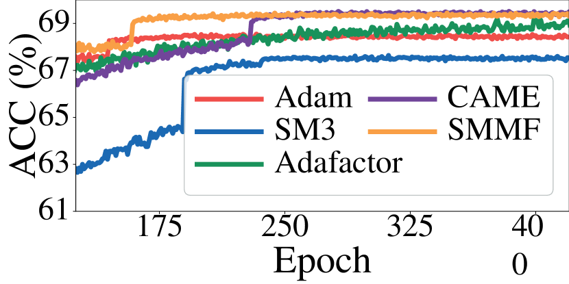
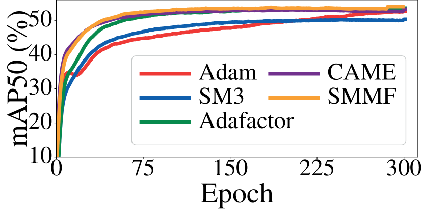
Figure 1: (Left) The validation top-1 accuracy of MobileNetV2 on ImageNet. (Right) The validation mAP50 of YOLOv5s on COCO of the five optimizers.

Object Detection. The third table of Table 1 summarizes the optimizer memory usage, end-to-end training (one-batch) memory usage, and the model performance metric (i.e., mAP50) of YOLOv5s and YOLOv5m on the COCO object detection task. Figure 1 (right) shows the mAP50 of YOLOv5s on COCO over training steps. Similar to image classification tasks, SMMF achieves comparable mAP50, e.g., 59.6 in YOLOv5m and 54.1 in YOLOv5s, over all the four optimizers with the lowest memory up to 78x reduction, e.g., 267 vs. 3.4 MiB. This result implies that YOLOv5s (65 MiB) can be trained on an off-the-shelf memory-constrained device, e.g., Coral Dev Micro (64 MiB) (Google 2022), along with other memory-efficient training methods such as gradient checkpointing (Chen et al. 2016).

These experiment results show that SMMF performs consistent and reliable optimization for both image classification and object detection tasks with different CNN models, taking the smallest memory compared to existing memory-efficient optimizers, i.e., Adafactor, SM3, and CAME.

Transformer Models and Tasks (Full-Trining)
(Optimizer and End-to-End Memory [GiB]), Model Performance
Dataset	WMT32k
Model	Adam			Adafactor			SM3			CAME			SMMF
Transformer	(	0.7,	1.4)	(	0.4,	1.1)	(	0.4,	1.1)	(	0.4,	1.1)	(	.01,	0.8)
(base)	6.6			6.6			7.8			6.6			6.7
Transformer	(	2.1,	4.2)	(	1.1,	3.2)	(	1.1,	3.2)	(	1.1,	3.2)	(	.04,	2.1)
(big)	6.9			6.6			7.9			7.5			6.8

Table 2: Full-training: the optimizer memory usage (GiB), including the $\boldsymbol{S}_{\boldsymbol{M}}$, end-to-end training (one-batch) memory usage (GiB) at 100 iterations, and test perplexity of the Transformer-base and big models on WMT32k.

5.2 Transformer-based Models and Tasks

Full-training. As shown in Table 2, SMMF achieves comparable perplexity with up to 70x smaller optimizer memory when full-training (i.e., training models from scratch) both the Transformer-base and big models. Since SMMF square-matricizes both the $1^{st}$ and $2^{nd}$ momentums and factorizes them, its memory usage is at least half lower than the other memory-efficient optimizers, i.e., Adafactor, SM3, and CAME. Given that most Transformer architectures consist of two-dimensional matrices, e.g., attention and linear layers, the memory reduction effect of SM3 that is good at compressing a high-rank tensor, becomes insignificant, making its memory usage similar to Adafactor and CAME. On the other hand, SMMF can effectively reduce memory required to factorize a two-dimensional matrix with square-matricization, e.g., saving 69% of memory for the embedding weight matrix of BERT, as the weight matrix in $\mathbb{R}^{30522\times 768}$ becomes $\mathbb{R}^{5087\times 4608}$. Although the square-matricization may spoil the gradient pattern of the Transformer’s weight parameters (Anil et al. 2019), SMMF performs comparable optimization (e.g., 6.7 perplexity for WMT32k) using much less memory by fully utilizing the intact latest gradient before it is compressed. It is possible by taking the proposed $decompression$$\rightarrow$$compression$ scheme that first reflects the intact gradient pattern, if any, to the momentum and then performs factorization, unlike existing optimizers, e.g., Adafactor, SM3, and CAME, which apply the $compression$$\rightarrow$$decompression$ scheme. Figure 2 (left) shows the test perplexity of the Transformer-base model full-trained on WMT32k from scratch.

Transformer Models and Tasks (Pre-Training)
(Optimizer and End-to-End Memory [GiB]), Model Performance
Dataset	Book Corpus & Wikipedia
Model	Adam			Adafactor			SM3			CAME			SMMF
BERT	(	2.5,	6.3)	(	1.3,	5.0)	(	1.3,	5.0)	(	1.3,	5.0)	(	.04,	3.8)
	16.1			30.6			27.5			20.1			20.4
GPT-2	(	2.6,	6.7)	(	1.3,	5.3)	(	1.3,	5.3)	(	1.3,	5.3)	(	.04,	4.0)
	19.2			NaN			19.4			19.1			19.2
T5	(	1.7,	4.2)	(	0.8,	3.4)	(	0.8,	3.4)	(	0.9,	3.4)	(	.03,	2.5)
	2.6			2.6			2.8			2.6			2.6

Table 3: Pre-training: the optimizer memory usage (GiB), including the $\boldsymbol{S}_{\boldsymbol{M}}$, end-to-end training (one-batch) memory usage (GiB) at 100 iterations, and test perplexity of BERT, GPT-2, and T5. We use Adam without the bias correction term to obtain lower perplexity.

Pre-training. Table 3 shows the optimizer memory usage including $\boldsymbol{S}_{\boldsymbol{M}}$, end-to-end training (one-batch) memory usage, and the perplexity of BERT, GPT-2, and T5 pre-trained for the BookCorpus & Wikipedia dataset. For GPT-2 pre-trained with Adafactor, we failed to obtain its perplexity since it diverged (NaN) even with multiple trials of various settings, e.g., different machines, hyper parameters, seeds, etc. On the other hand, SMMF performs competitive optimization for all pre-training of BERT, GPT-2, and T5 using up to 60x lower optimizer memory. Figure 2 (right) shows that SMMF (yellow) curtails the optimizer memory usage in the pre-training of BERT about 1.26 GiB (from 1.3 to 0.04 GiB) while exhibiting the similar test perplexity trajectory to CAME (purple) taking much more memory to maintain the similar optimization performance. Overall, Adafactor, CAME, and SMMF show similar perplexity trajectories, confirming that SMMF retains the optimization performance in pre-training of Transformers with the lowest memory, enabled by 1) square-matricization of any rank (shape) of momentums (e.g., a vector, matrix, tensor, etc.) and 2) the $decompression$$\rightarrow$$compression$ scheme that uses the uncompressed gradients at the current update step. They jointly allow it to pre-train Transformers aptly during a massive number of pre-training steps by persistently conducting effective and efficient optimization over a long time horizon.

That being said, SMMF also exhibits some occasional loss spike (Takase et al. 2024; Zhang and Xu 2023) at the early steps of optimization (training), which stabilizes as the training proceeds. It is a well-known phenomenon that commonly occurs in the pre-training of many large language models (Raffel et al. 2020; Radford et al. 2019) optimized with existing optimizers, such as Adam, Adafactor, SM3, and CAME. We discuss it in more detail in Section 6.

Fine-tuning. Table 4 summarizes the optimization memory usage including $\boldsymbol{S}_{\boldsymbol{M}}$, end-to-end training(one-batch) memory usage, and the model performance of GPT-2, T5-small, and LLaMA-7b, which are fine-tuned for the QNLI, MNLI, QQP, STSB, and MRPC datasets from pre-trained models. As shown in the table, SMMF achieves comparable model performance in the six datasets compared to the other four optimizers with the lowest memory usage. For instance, SMMF provides similar accuracy (90.6%) for GPT-2 on QQP compared to CAME, using much smaller optimizer and end-to-end training memory, respectively (16 vs. 489 MiB and 0.96 vs. 1.43 GiB). It demonstrates that SMMF is also apt at fine-tuning Transformer models, which entails delicate and intricate updates of weight parameters, otherwise likely to degrade the learning performance for downstream tasks. In practice, it suggests that some Transformer models, such as T5, would be fine-tuned on a low-end device, e.g., Raspberry Pi Zero (0.5 GiB), with similar model performance to CAME (i.e., 83.0% vs. 82.8%), as SMMF curtails the end-to-end training memory requirement of fine-tuning down to 0.47 GiB. On the other way around, SMMF can scale up training of Transformers by enabling memory-efficient optimization of enormous Transformer models that require a gigantic amount of memory, e.g., hundreds of GiB.

Similar to the CNN-based models and tasks, the experimental results of Transformers demonstrate that SMMF steadily performs competitive optimization for a wide range of Transformer models, tasks, and training methods (i.e., full-, pre-, and fine-tuning) with the smallest memory usage.

Transformer Models and Tasks (Fine-Tuning)
(Optimizer Memory [MiB] and End-to-End Memory [GiB]), Model Performance
Optimizer	Model	QNLI (ACC)				MNLI (ACC)				QQP (ACC)				STSB (Pearson)				MRPC (ACC)
Adam		(	957,	1.89)	84.5	(	952,	1.89)	72.4	(	973,	1.89)	86.4	(	962,	1.89)	83.2	(	861,	1.89)	81.4
Adafactor		(	478,	1.43)	74.7	(	478,	1.43)	71.7	(	488,	1.43)	80.1	(	481,	1.43)	84.4	(	481,	1.43)	82.6
SM3	GPT-2	(	478,	1.43)	88.0	(	478,	1.43)	81.1	(	487,	1.43)	88.8	(	481,	1.43)	84.1	(	481,	1.43)	83.3
CAME		(	468,	1.43)	88.6	(	479,	1.43)	81.9	(	489,	1.43)	90.6	(	481,	1.43)	86.4	(	478,	1.43)	83.3
SMMF		(	16,	0.96)	88.9	(	16,	0.96)	82.2	(	16,	0.96)	90.6	(	16,	0.96)	83.8	(	16,	0.96)	81.6
Adam		(	464,	0.92)	88.4	(	464,	0.92)	77.5	(	434,	0.92)	86.8	(	456,	0.92)	84.7	(	464,	0.92)	77.5
Adafactor		(	233,	0.70)	90.1	(	233,	0.70)	80.3	(	233,	0.70)	88.7	(	233,	0.70)	87.9	(	233,	0.70)	80.3
SM3	T5	(	233,	0.70)	88.8	(	233,	0.70)	79.4	(	233,	0.70)	88.1	(	233,	0.70)	79.4	(	233,	0.70)	79.4
CAME	(small)	(	233,	0.70)	90.7	(	234,	0.70)	83.0	(	233,	0.70)	90.4	(	233,	0.70)	87.5	(	234,	0.70)	83.0
SMMF		(	8,	0.47)	90.6	(	8,	0.47)	82.8	(	8,	0.47)	90.2	(	8,	0.47)	84.7	(	8,	0.47)	82.8
Adam		(	153,	24.9)	93.0	(	153,	24.9)	87.5	(	153,	24.9)	84.4	(	153,	24.9)	96.6	(	153,	24.9)	90.6
Adafactor		(	86,	24.9)	93.8	(	86,	24.9)	84.4	(	86,	24.9)	93.0	(	86,	24.9)	96.3	(	86,	24.9)	85.9
SM3	LLaMA-7b	(	86,	24.9)	65.6	(	86,	24.9)	64.8	(	86,	24.9)	71.9	(	86,	24.9)	34.9	(	86,	24.9)	70.3
CAME		(	86,	24.9)	69.5	(	86,	24.9)	43.0	(	86,	24.9)	75.8	(	86,	24.9)	34.8	(	86,	24.9)	70.3
SMMF		(	3.9,	24.8)	91.4	(	3.9,	24.8)	87.5	(	3.9,	24.8)	90.6	(	3.9,	24.8)	96.5	(	3.9,	24.8)	89.8

Table 4: Fine-tuning: the optimizer and end-to-end training (one-batch) memory usage [MiB, GiB] at 100 iterations including $\boldsymbol{S}_{\boldsymbol{M}}$, and the performance of GPT-2, T5-small, and LLaMA-7b fine-tuned on QNLI, MNLI, QQP, STSB, and MRPC.

Optimization Time (ms) for a Single Training Step (Iteration)
Model	Adam		Adafactor		SM3		CAME		SMMF
MobileNetV2	127$\pm$	16	168$\pm$	16	140$\pm$	17	160$\pm$	17	205$\pm$	13
ResNet-50	273$\pm$	16	316$\pm$	14	286$\pm$	14	307$\pm$	20	349$\pm$	15
Transformer-base	129$\pm$	7	160$\pm$	7	134$\pm$	7	156$\pm$	7	171$\pm$	7
Transformer-big	321$\pm$	18	372$\pm$	18	325$\pm$	18	369$\pm$	18	389$\pm$	18

Table 5: The single optimization time (milliseconds) per step of the four optimizers, and SMMF (8-bit format $\boldsymbol{S_{M}}$ in Algorithm 3 and 4): 1) MobileNetV2 and ResNet-50 on ImageNet, and 2) Transformer-base and big on WMT32k.

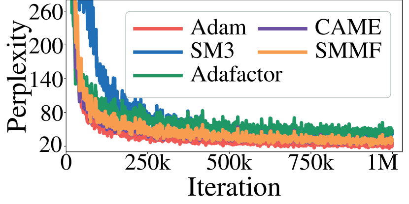
Figure 2: The test perplexity of the Transformer-base model on WMT32k during full-training steps (Left) and BERT on BookCorpus & Wikipedia during pre-training steps (Right)

5.3 Optimization Time Measurement

Table 5 shows the optimization time measured for a single training step of the five optimizers when training MobileNetV2 and ResNet-50 on ImageNet, and Transformer-base and big on WMT32k. Except for Adam, the four optimizers take similar optimization times, where SMMF takes a little more time than the other three. That is because it trades off the memory space and optimization time, i.e., the time required for square-matricization and the sign matrix operations for the $1^{st}$ momentum (Algorithms 3 and 4). However, SMMF offers huge memory reduction compared to the amount of the increased optimization time, e.g., 7.9x memory reduction vs. 1.2x time increase for Adam and SMMF with the 8-bit format $\boldsymbol{S_{M}}$ in Algorithms 3 and 4 applied to Transformer-big on WMT32k, and 7.8x vs. 1.6x for Adam and SMMF with $\boldsymbol{S_{M}}$ applied to ResNet-50 on ImageNet.

6 Limitations and Discussions

Overhead of Binary Signs. It is not easy to effectively factorize the $1^{st}$ momentum $\boldsymbol{M}$ having negative elements. While SMMF circumvents this by storing the binary sign matrix (1-bit) that is much smaller than the original matrix (32-bit), there are some methods that can further reduce the memory required to store the sign matrix. For instance, Binary Matrix Factorization (Kumar et al. 2019; Shi, Wang, and Shi 2014) can be employed to factorize the binary matrix into two lower-rank matrices, reducing the memory space for storing the binary matrix with a high restoration rate.

Optimization Time. Section 3.3 finds that the time complexity of SMMF is similar to existing memory-efficient optimizers, e.g., Adafactor, showing that SMMF effectively saves a significant amount of memory (up to 96%) compared to them with slightly increased optimization time.

Loss Spike at Initial Training Steps. We observe some loss spike at the initial training steps, especially in Transformer models, which is a well-known issue commonly observed in other works (Takase et al. 2024; Zhang and Xu 2023) and many optimizers, i.e., Adam (with the bias correction term), Adafactor, SM3, and CAME. With appropriate hyper-parameter tuning, e.g., learning rate and weight-decay, it can be stabilized as the training proceeds, like other optimizers.

Extremely Large Models and Other Tasks. Due to the limited computing resources, we have not been able to experiment SMMF with extremely large models, e.g, GPT-4 (OpenAI et al. 2024), LLaMA-2 70B (Touvron et al. 2023b), and diffusion models (Rombach et al. 2022). From our theoretical study and empirical result, we expect SMMF to perform competitive optimization with them. We hope to have a chance to test SMMF with them.

7 Conclusion

We introduce SMMF, a memory-efficient optimizer that decreases the memory requirement of adaptive learning rate optimization methods, e.g., Adam and Adafactor. Given arbitrary-rank momentum tensors, SMMF reduces the optimization memory usage through the proposed square-matricization and matrix compression of the first and second momentums. The empirical evaluation shows that SMMF reduces up to 96% of optimization memory when compared to existing memory-efficient optimizers, i.e., Adafactor, SM3, and CAME, with competitive optimization performance on various models (i.e., CNNs and Transformers) and tasks (i.e., image classification, object detection, and NLP tasks over full-training, pre-training, and fine-tuning). Our analysis of regret bound proves that SMMF converges in a convex function with a similar bound of AdamNC.

Appendix A Relative Training Time comparison

As described in Table 5, SMMF trades off training time for memory efficiency to minimize the substantial memory consumption incurred by optimizer states, such as momentum tensors. This means that training time may increase slightly to achieve higher memory efficiency. While we have already compared the training time of the five optimizers, including Adam, Adafactor, SM3, CAME, and SMMF, we present detailed training time figures for two tasks: image classification of MobileNetV2 on ImageNet and full-training a Transformer-base on WMT32k. These results demonstrate that SMMF offers significant memory saving despite a slight increase in training time.

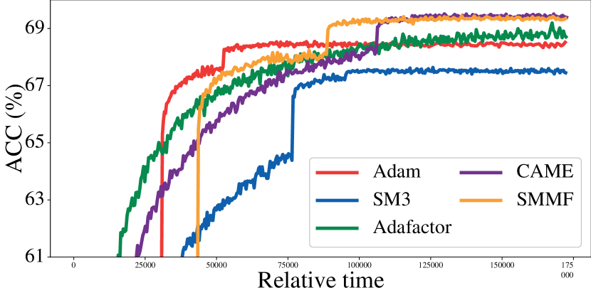
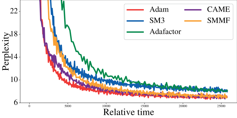
Figure 3: (Left) The validation top-1 accuracy of MobileNetV2 on ImageNet. (Right) The test perplexity of the Transformer-base model on WMT32k during full-training steps.

The graphs, based on measurements from the Wandb  platform, show the training time for two tasks, i.e., image classification and full-training . The left graph corresponds to training MobileNetV2 on ImageNet, and the right graph corresponds to training the Transformer-base model on WMT32k. As can be seen from both graphs, SMMF is slower than Adam (Figures 1 and 2 for reference). This is because SMMF trades off computation and memory. Although SMMF is on average 1.4 times slower than Adam (Table 5 for reference), it compresses memory by approximately 96%, making it an algorithm that significantly reduces memory usage relative to its speed.

Appendix B NNMF (Non-Negative Matrix Factorization)

Algorithm 5 Non-Negative Matrix Factorization (NNMF) (Shazeer and Stern 2018)

 Input: Non-negative matrix $\boldsymbol{M}\in\mathbb{R}^{n\times m}$

 Output: Factorized two vectors, $\boldsymbol{r}\in\mathbb{R}^{n\times 1}$ and $\boldsymbol{c}\in\mathbb{R}^{1\times m}$

 $\boldsymbol{r}=\boldsymbol{M}\boldsymbol{1}_{m}$

 $\boldsymbol{c}=\boldsymbol{1}_{n}^{\top}\boldsymbol{M}$

 $\boldsymbol{c}=\dfrac{\boldsymbol{c}}{\boldsymbol{c}\boldsymbol{1}_{m}}$

Appendix C Proof of Theorem 3.1

Proof.

Let $N^{\prime}=\prod_{r=1}^{d-2}n_{r}$. Then we have:

$$\prod_{r=1}^{d-2}n_{r}(n_{d-1}+n_{d})=N^{\prime}(n_{d-1}+n_{d})$$ (3)

Since $N=N^{\prime}(n_{d-1}\times n_{d})$, we can rewrite the above equation:

$$\prod_{r=1}^{d-2}n_{r}(n_{d-1}+n_{d}) =N\dfrac{(n_{d-1}+n_{d})}{n_{d-1}\times n_{d}}$$ (4)

$$=N\left(\dfrac{1}{n_{d}}+\dfrac{1}{n_{d-1}}\right)$$ (5)

From Lemma C.1, we have the function, $f(n_{d},n_{d-1})=\frac{1}{n_{d}}+\frac{1}{n_{d-1}}$, which is symmetric with respect to $n_{d}=n_{d-1}$ and a convex function where the Hessian matrix is positive definite and asymptotically converges to zero as $n_{d}$ and $n_{d-1}$ grow. It means the function decreases as $n_{d-1}\simeq n_{d}$ (i.e., $\arg\min(n_{d-1}-n_{d}))$ and both $n_{d}$ and $n_{d-1}$ increase. ∎

Lemma C.1.

Given $f(x,y)=\frac{1}{x}+\frac{1}{y}$ where $x,y>0$, then the function $f(x,y)$ is a convex function.

Proof.

In order to prove that a function $f(x,y)$ is a convex function, we have to show the Hessian matrix of $f(x,y)$ is positive semi-definite. The following is the Hessian of the function.

$$\boldsymbol{H}=\begin{bmatrix}\dfrac{\partial^{2}f}{\partial x^{2}}&\dfrac{\partial^{2}f}{\partial x\partial y}\\ \dfrac{\partial^{2}f}{\partial y\partial x}&\dfrac{\partial^{2}f}{\partial y^{2}}\\ \end{bmatrix}=\begin{bmatrix}\dfrac{2}{x^{3}}&0\\ 0&\dfrac{2}{y^{3}}\\ \end{bmatrix}$$ (6)

Since $x$ and $y$ are greater than 0, the eigenvalues of the Hessian matrix, $\boldsymbol{H}$, are positive, which means the matrix is positive definite and the function $f(x,y)$ is a convex function. ∎

Appendix D Proof of Theorem 3.2

Proof.

Let the function, $f_{-}(n,m)$, be $m-n$ and the function, $f_{+}(n,m)$ be $m+n$. As rewritten in Theorem D.1 proof, $f_{-}(n,m)$ is $f_{-}(m)=m-\frac{N}{m}$ and $f_{+}(n,m)$ is $f_{+}(m)=m+\frac{m}{m}$. Since the given conditions are under the condition of Theorem D.1, Theorem 3.2 is proved. Also, we can prove the theorem using Lemmas D.1 and D.2. The both lemmas show that the two functions, $f_{-}(n,m)$ and $f_{+}(n,m)$ are strictly monotonically increasing function under the given conditions, which means that the directions to the minima are equal (i.e., the sign values of each function’s gradient are positive) and minimizing one function leads to minimizing another function. ∎

Theorem D.1.

Given $n_{r},n$, and $m\in\mathbb{R}^{+}$, $r\in[1,d]$, $N=\prod_{r=1}^{d}n_{r}=nm$, and $n\leq m$, then the following holds:

$$\arg\min_{n,m}(m-n)=\arg\min_{n,m}(m+n)$$ (7)

Proof.

In order to prove Theorem D.1, $n$ and $m$ at the minima of the function, $f_{-}(n,m)=m-n$, and the function, $f_{+}(n,m)=m+n$, should be same under the given condition. Since $n$ depends on the $m$ and given constant $N$, the function, $f_{-}(n,m)$, becomes $f_{-}(m)=m-\frac{N}{m}$ and the function, $f_{+}(n,m)$, becomes $f_{+}(m)=m+\frac{N}{m}$. For the function, $f_{-}(m)$, $m$ at the minima of the function is always $\sqrt{N}$ since the function is strictly increasing function via Lemma D.1, and the minima of the function is $0$ where $m=\sqrt{N}=n$ since the function is greater than or equals to $0$ under the given condition. Fot the function, $f_{+}(m)$, $m$ at the minima of the function is also always $\sqrt{N}$ since the function is a convex function and has only one $m$ which satisfies $\frac{df_{+}(m)}{dm}=0$ via Lemma D.2. ∎

Lemma D.1.

Given $N\in\mathbb{Z}$ and $0<x<\infty$, then the function, $f(x):\mathbb{R}\rightarrow\mathbb{R}=x-\frac{N}{x}$, is a strictly increasing function.

Proof.

In order to determine that the function, $f(x)$, is strictly increasing with respect to $x$, the following should be satisfied:

$$\dfrac{df(x)}{dx}>0$$ (8)

The differentiation of the function, $f(x)=x-\frac{N}{x}$, with respect to $x$ is:

$$\dfrac{df(x)}{dx}=1+\dfrac{N}{x^{2}}$$ (9)

Under the given condition, $0<x<\infty$, Equation 9 is always positive. ∎

Lemma D.2.

Given $N\in\mathbb{Z}$ and $0<x<\infty$, the function, $f(x):\mathbb{R}\rightarrow\mathbb{R}=x+\frac{N}{x}$, is a convex function where the number of $x$ which satisfies $\frac{df(x)}{dx}=0$ is one.

Proof.

In order to show that the function, $f(x)=x+\frac{N}{x}$, is a convex function, the second derivative of the function should be greater than or equal to zero:

$$\dfrac{d^{2}f(x)}{dx^{2}}=\dfrac{2N}{x^{3}}$$ (10)

Under the given condition, $0<x<\infty$, Equation 10 is always greater than zero.

In order to prove that the number of $x$ which satisfies $\frac{df(x)}{dx}=0$ is one, we need the derivative of the function, $f(x)$:

$$\dfrac{df(x)}{dx}=1-\dfrac{N}{x^{2}}=0$$ (11)

The $x$ which satisfies Equation 11 are $\pm\sqrt{N}$, but the feasible $x$ is $x=\sqrt{N}$ under the given condition, $0<x<\infty$, so that the number of possible $x$ is one. ∎

Appendix E Proof of Theorem 4.1

Proof.

From Lemma E.2 we have:

$$R(T)=\sum_{t=1}^{T}(f_{t}(\boldsymbol{w}_{t})-f_{t}(\boldsymbol{w}^{*}))\leq\sum_{t=1}^{T}\sum_{i=1}^{d}f(\boldsymbol{w}_{t})_{i}(\boldsymbol{w}_{t}-\boldsymbol{w}^{*})_{i}$$ (12)

From the update rule of Algorithm 1 without $\epsilon$ for simple proof, we have:

$$\boldsymbol{w}_{t+1} =\boldsymbol{w}_{t}-\eta_{t}\dfrac{\boldsymbol{m}_{t}}{\sqrt{\boldsymbol{v}_{t}}}$$ (13)

$$=\boldsymbol{w}_{t}-\eta_{t}\left\{\dfrac{\beta_{1,t}}{\sqrt{\boldsymbol{v}_{t}}}\boldsymbol{m}_{t-1}+\dfrac{(1-\beta_{1,t})}{\sqrt{\boldsymbol{v}_{t}}}\boldsymbol{g}_{t}\right\}$$ (14)

In order to make the form of Equation 12, we subtract $\boldsymbol{w}^{*}$ and square both sides of the equation, and write the equation focusing on the $i^{th}$ element in the vector $\boldsymbol{w}_{t}$.

$$(\boldsymbol{w}_{t+1,i}-\boldsymbol{w}_{,i}^{*})^{2} =(\boldsymbol{w}_{t,i}-\boldsymbol{w}_{,i}^{*})^{2}-2\eta_{t}\left\{\dfrac{\beta_{1,t}}{\sqrt{\boldsymbol{v}_{t,i}}}\boldsymbol{m}_{t-1,i}+\dfrac{(1-\beta_{1,t})}{\sqrt{\boldsymbol{v}_{t,i}}}\boldsymbol{g}_{t,i}\right\}(\boldsymbol{w}_{t,i}-\boldsymbol{w}_{,i}^{*})$$ (15)

$$+\eta_{t}^{2}\left(\dfrac{\boldsymbol{m}_{t,i}}{\sqrt{\boldsymbol{v}_{t,i}}}\right)^{2}$$ (16)

By rearranging the equation, we have:

$$\boldsymbol{g}_{t,i}(\boldsymbol{w}_{t,i}-\boldsymbol{w}_{,i}^{*}) =\dfrac{\sqrt{\boldsymbol{v}_{t,i}}}{2\eta_{t}(1-\beta_{1,t})}\left\{(\boldsymbol{w}_{t,i}-\boldsymbol{w}_{,i}^{*})^{2}-(\boldsymbol{w}_{t+1,i}-\boldsymbol{w}_{,i}^{*})^{2}\right\}$$ (17)

$$+\dfrac{\eta_{t}\sqrt{\boldsymbol{v}_{t,i}}}{2(1-\beta_{1,t})}\left(\dfrac{\boldsymbol{m}_{t,i}}{\sqrt{\boldsymbol{v}_{t,i}}}\right)^{2}-\dfrac{\beta_{1,t}}{(1-\beta_{1,t})}\hat{\boldsymbol{m}}_{t-1,i}(\boldsymbol{w}_{t,i}-\boldsymbol{w}_{,i}^{*})$$ (18)

By applying Young’s inequality, we have:

$$\boldsymbol{g}_{t,i}(\boldsymbol{w}_{t,i}-\boldsymbol{w}_{,i}^{*}) \leq\dfrac{\sqrt{\boldsymbol{v}_{t,i}}}{2\eta_{t}(1-\beta_{1,t})}\left\{(\boldsymbol{w}_{t,i}-\boldsymbol{w}_{,i}^{*})^{2}-(\boldsymbol{w}_{t+1,i}-\boldsymbol{w}_{,i}^{*})^{2}\right\}$$ (19)

$$+\dfrac{\beta_{1,t}}{2\eta_{t-1}(1-\beta_{1,t})}(\boldsymbol{w}_{,i}^{*}-\boldsymbol{w}_{t,i})^{2}\sqrt{\boldsymbol{v}_{t-1,i}}+\dfrac{\eta_{t-1}\beta_{1,t}}{2(1-\beta_{1,t})}\dfrac{\hat{\boldsymbol{m}}_{t-1,i}^{2}}{\sqrt{\boldsymbol{v}_{t-1,i}}}$$ (20)

$$+\dfrac{\eta_{t}\sqrt{\boldsymbol{v}_{t,i}}}{2(1-\beta_{1,t})}\left(\dfrac{\boldsymbol{m}_{t,i}}{\sqrt{\boldsymbol{v}_{t,i}}}\right)^{2}$$ (21)

Since we want to compute regret, we compute the below inequality by applying Lemma E.5 and Lemma E.6:

$$\sum_{t=1}^{T}\sum_{i=1}^{d}\boldsymbol{g}_{t,i}(\boldsymbol{w}_{t,i}-\boldsymbol{w}_{,i}^{*}) \leq\sum_{t=1}^{T}\sum_{i=1}^{d}\dfrac{\sqrt{\boldsymbol{v}_{t,i}}}{2\eta_{t}(1-\beta_{1,t})}\left\{(\boldsymbol{w}_{t,i}-\boldsymbol{w}_{,i}^{*})^{2}-(\boldsymbol{w}_{t+1,i}-\boldsymbol{w}_{,i}^{*})^{2}\right\}$$ (22)

$$+\sum_{t=1}^{T}\sum_{i=1}^{d}\dfrac{\beta_{1,t}}{2\eta_{t-1}(1-\beta_{1,t})}(\boldsymbol{w}_{,i}^{*}-\boldsymbol{w}_{t,i})^{2}\sqrt{\boldsymbol{v}_{t-1,i}}$$ (23)

$$+\dfrac{\zeta_{1}\zeta_{2}(1+\beta_{1})\sqrt{d}}{(1-\beta_{1})^{3}}\sqrt{\sum_{i=1}^{d}\sum_{t=1}^{T}\boldsymbol{g}_{t,i}^{2}}$$ (24)

under the given condition $\beta_{1}=\beta_{1,1}$ and $\beta_{1,t}\leq\beta_{1}$.

By rearranging the inequality and using the condition $\eta_{t-1}\sqrt{\boldsymbol{v}_{t,i}}\geq\eta_{t}\sqrt{\boldsymbol{v}_{t-1,i}}$, we have:

$$\sum_{t=1}^{T}\sum_{i=1}^{d}\boldsymbol{g}_{t,i}(\boldsymbol{w}_{t,i}-\boldsymbol{w}_{,i}^{*}) \leq\sum_{i=1}^{d}\dfrac{1}{2\eta_{1}(1-\beta_{1,1})}(\boldsymbol{w}_{1,i}-\boldsymbol{w}_{,i}^{*})^{2}\sqrt{\boldsymbol{v}_{1,i}}$$ (25)

$$+\sum_{t=2}^{T}\sum_{i=1}^{d}\dfrac{1}{2(1-\beta_{1,t})}(\boldsymbol{w}_{t,i}-\boldsymbol{w}_{,i}^{*})^{2}\left(\dfrac{\sqrt{\boldsymbol{v}_{t,i}}}{\eta_{t}}-\dfrac{\sqrt{\boldsymbol{v}_{t-1,i}}}{\eta_{t-1}}\right)$$ (26)

$$+\sum_{t=1}^{T}\sum_{i=1}^{d}\dfrac{\beta_{1,t}}{2\eta_{t}(1-\beta_{1,t})}(\boldsymbol{w}_{,i}^{*}-\boldsymbol{w}_{t,i})^{2}\sqrt{\boldsymbol{v}_{t,i}}$$ (27)

$$+\dfrac{\zeta_{1}\zeta_{2}(1+\beta_{1})\sqrt{d}}{(1-\beta_{1})^{3}}\sqrt{\sum_{i=1}^{d}\sum_{t=1}^{T}\boldsymbol{g}_{t,i}^{2}}$$ (28)

Using the assumption $\lvert\lvert\boldsymbol{w}_{t}-\boldsymbol{w}^{*}\rvert\rvert_{2}\leq D$ and $\lvert\lvert\boldsymbol{w}_{t}-\boldsymbol{w}^{*}\rvert\rvert_{\infty}\leq D_{\infty}$, we have:

$$R(T) \leq\dfrac{D^{2}}{2\eta_{T}(1-\beta_{1})}\sum_{i=1}^{d}\sqrt{\boldsymbol{v}_{T,i}}$$ (29)

$$+\sum_{t=1}^{T}\sum_{i=1}^{d}\dfrac{\beta_{1,t}}{2\eta_{t}(1-\beta_{1,t})}D_{\infty}^{2}\sqrt{\boldsymbol{v}_{t,i}}$$ (30)

$$+\dfrac{\zeta_{1}\zeta_{2}(1+\beta_{1})\sqrt{d}}{(1-\beta_{1})^{3}}\sqrt{\sum_{i=1}^{d}\sum_{t=1}^{T}\boldsymbol{g}_{t,i}^{2}}$$ (31)

∎

Lemma E.1.

Let a function $f:\mathbb{R}^{d}\rightarrow\mathbb{R}$ be a convex function. Given $\forall\boldsymbol{x}\in\mathbb{R}^{d}$, $\forall\boldsymbol{y}\in\mathbb{R}^{d}$, and $\rho\in[0,1]$, then the following holds:

$$\rho f(\boldsymbol{x})+(1-\rho)f(\boldsymbol{y})\geq f(\rho\boldsymbol{x}+(1-\rho)\boldsymbol{y})$$ (32)

Lemma E.2.

Let a function $f:\mathbb{R}^{d}\rightarrow\mathbb{R}$ be a convex function. Given $\forall\boldsymbol{x}\in\mathbb{R}^{d}$ and $\forall\boldsymbol{y}\in\mathbb{R}^{d}$, then the following holds:

$$f(\boldsymbol{y}) \geq f(\boldsymbol{x})+\nabla f(\boldsymbol{x})^{\top}(\boldsymbol{y}-\boldsymbol{x})$$ (33)

$$=f(\boldsymbol{x})+\sum_{i=1}^{d}\nabla f(\boldsymbol{x})_{i}(\boldsymbol{y}-\boldsymbol{x})_{i}$$ (34)

where $\nabla f(\boldsymbol{x})$ is the $i^{th}$ element in the vector $\nabla f(\boldsymbol{x})$ and $(\boldsymbol{y}-\boldsymbol{x})_{i}$ is the $i^{th}$ element in the vector.

Lemma E.3.

Let $\hat{\boldsymbol{m}}_{t}$, $\hat{\boldsymbol{v}}_{t}$, $\boldsymbol{m}_{t}$, $\boldsymbol{v}_{t}$, and $\boldsymbol{g}_{t}$ are respectively vectorized $\hat{\boldsymbol{M}}_{t}$, $\hat{\boldsymbol{V}}_{t}$, $\boldsymbol{M}_{t}$, $\boldsymbol{V}_{t}$, and $\boldsymbol{G}_{t}$, in Algorithm 1. Given $\beta_{1,j}$ and $\beta_{2,j}$ at $j=t$ in the algorithm, the followings are satisfied:

$$\hat{\boldsymbol{m}}_{t}-\boldsymbol{m}_{t} =\boldsymbol{e}_{m,t}$$ (35)

$$\hat{\boldsymbol{v}}_{t}-\boldsymbol{v}_{t} =\boldsymbol{e}_{v,t}$$ (36)

$$\hat{\boldsymbol{g}}_{m,t} =\left(\boldsymbol{g}_{t}+\dfrac{\boldsymbol{e}_{m,t}}{(1-\beta_{1,t})}\right)$$ (37)

$$\hat{\boldsymbol{g}}_{v,t} =\left(\boldsymbol{g}_{t}^{2}+\dfrac{\boldsymbol{e}_{v,t}}{(1-\beta_{2,t})}\right)$$ (38)

$$\hat{\boldsymbol{m}}_{t} =\sum_{j=1}^{t}(1-\beta_{1,j})\prod_{k=1}^{t-j}\beta_{1,t-k+1}\hat{\boldsymbol{g}}_{m,j}=\boldsymbol{m}_{t}+\boldsymbol{e}_{m,t}$$ (39)

$$\hat{\boldsymbol{v}}_{t} =\sum_{j=1}^{t}(1-\beta_{2,j})\prod_{k=1}^{t-j}\beta_{2,t-k+1}\hat{\boldsymbol{g}}_{m,j}=\boldsymbol{v}_{t}+\boldsymbol{e}_{v,t}$$ (40)

where $\boldsymbol{e}_{m,t}$ and $\boldsymbol{e}_{v,t}$ are $decompression\rightarrow compression$ errors at $t\in[1,T]$ such that $\hat{\boldsymbol{m}}_{t}-\boldsymbol{m}_{t}=\boldsymbol{e}_{m,t}$ and $\hat{\boldsymbol{v}}_{t}-\boldsymbol{v}_{t}=\boldsymbol{e}_{v,t}$.

Proof.

Following Algorithm 1, we have:

$$\boldsymbol{m}_{1} =(1-\beta_{1,1})\boldsymbol{g}_{1}$$ (41)

$$\hat{\boldsymbol{m}}_{1} =\boldsymbol{m}_{1}+\boldsymbol{e}_{m,1}=(1-\beta_{m,1})\left(\boldsymbol{g}_{1}+\dfrac{\boldsymbol{e}_{m,1}}{(1-\beta_{1,1})}\right)$$ (42)

$$=(1-\beta_{1,1})\hat{\boldsymbol{g}}_{m,1}$$ (43)

$$\boldsymbol{m}_{2} =\beta_{1,2}\hat{\boldsymbol{m}}_{1}+(1-\beta_{1,2})\boldsymbol{g}_{2}$$ (44)

$$\hat{\boldsymbol{m}}_{2} =\boldsymbol{m}_{2}+\boldsymbol{e}_{m,2}$$ (45)

$$=\beta_{1,2}\hat{\boldsymbol{m}}_{1}+(1-\beta_{m,2})\hat{\boldsymbol{g}}_{m,2}$$ (46)

$$\vdots$$

$$\hat{\boldsymbol{m}}_{t} =\sum_{j=1}^{t}(1-\beta_{1,j})\prod_{k=1}^{t-j}\beta_{1,t-k+1}\hat{\boldsymbol{g}}_{m,j}$$ (47)

We can apply the proof to $\hat{\boldsymbol{v}}_{t}$ momentum using similar way. ∎

Lemma E.4.

Let $j$ be in $[1:\tau]$ (from initial step to current step) and let $\tilde{\boldsymbol{e}}_{m,j}$ and $\tilde{\boldsymbol{e}}_{v,j}$ follow:

$$\tilde{\boldsymbol{e}}_{m,j} =\begin{dcases*}\boldsymbol{0},&if $j=\tau$\\ \boldsymbol{e}_{m,j},&otherwise\end{dcases*}$$ (48)

$$\tilde{\boldsymbol{e}}_{v,j} =\begin{dcases*}\boldsymbol{0},&if $j=\tau$\\ \boldsymbol{e}_{v,j},&otherwise\end{dcases*}$$ (49)

Then the following holds:

$$\tilde{\boldsymbol{g}}_{m,j} =\boldsymbol{g}_{j}+\frac{\tilde{\boldsymbol{e}}_{m,j}}{(1-\beta_{1,j})}$$ (50)

$$\tilde{\boldsymbol{g}}_{v,j} =\boldsymbol{g}_{j}^{2}+\frac{\tilde{\boldsymbol{e}}_{v,j}}{(1-\beta_{2,j})}$$ (51)

$$\boldsymbol{m}_{t} =\sum_{j=1}^{t}(1-\beta_{1,j})\prod_{k=1}^{t-j}\beta_{1,t-k+1}\tilde{\boldsymbol{g}}_{m,j}$$ (52)

$$\boldsymbol{v}_{t} =\sum_{j=1}^{t}(1-\beta_{2,j})\prod_{k=1}^{t-j}\beta_{2,t-k+1}\tilde{\boldsymbol{g}}_{m,j}$$ (53)

Proof.

From Equation 39, we have:

$$\boldsymbol{m}_{t}=\sum_{j=1}^{t}(1-\beta_{1,j})\prod_{k=1}^{t-j}\beta_{1,t-k+1}\hat{\boldsymbol{g}}_{m,j}-\boldsymbol{e}_{m,t}$$ (54)

By the definition of $\hat{\boldsymbol{g}}_{m,j}$ at Lemma E.3, we have:

$$\boldsymbol{m}_{t} =\sum_{j=1}^{t}(1-\beta_{1,j})\prod_{k=1}^{t-j}\beta_{1,t-k+1}\left(\boldsymbol{g}_{j}+\dfrac{\boldsymbol{e}_{m,j}}{(1-\beta_{1,j})}\right)-\boldsymbol{e}_{m,t}$$ (55)

$$=\sum_{j=1}^{t}(1-\beta_{1,j})\prod_{k=1}^{t-j}\beta_{1,t-k+1}\boldsymbol{g}_{j}+\sum_{j=1}^{t}\prod_{k=1}^{t-j}\beta_{1,t-k+1}\boldsymbol{e}_{m,j}-\boldsymbol{e}_{m,t}$$ (56)

$$=\sum_{j=1}^{t}(1-\beta_{1,j})\prod_{k=1}^{t-j}\beta_{1,t-k+1}\boldsymbol{g}_{j}+\sum_{j=1}^{t-1}\prod_{k=1}^{t-j}\beta_{1,t-k+1}\boldsymbol{e}_{m,j}$$ (57)

By introducing the definition of $\tilde{\boldsymbol{e}}_{m,j}$, we have:

$$\boldsymbol{m}_{t} =\sum_{j=1}^{t}(1-\beta_{1,j})\prod_{k=1}^{t-j}\beta_{1,t-k+1}\boldsymbol{g}_{j}+\sum_{j=1}^{t}\prod_{k=1}^{t-j}\beta_{1,t-k+1}\tilde{\boldsymbol{e}}_{m,j}$$ (58)

$$=\sum_{j=1}^{t}(1-\beta_{1,j})\prod_{k=1}^{t-j}\beta_{1,t-k+1}\tilde{\boldsymbol{g}}_{m,j}$$ (59)

We can apply the proof to $\boldsymbol{v}_{t}$ using similar way. ∎

Lemma E.5.

Given the conditions and notations in Theorem 4.1, we have:

$$\sum_{i=1}^{d}\sum_{t=1}^{T}\eta_{t}\dfrac{\boldsymbol{m}_{t,i}^{2}}{\sqrt{\boldsymbol{v}_{t,i}}} \leq\dfrac{2\zeta_{1}\zeta_{2}}{(1-\beta_{1})^{2}}\sqrt{\sum_{i=1}^{d}\sum_{t=1}^{T}\boldsymbol{g}_{t,i}^{2}}$$ (60)

Proof.

$$\sum_{i=1}^{d}\sum_{t=1}^{T}\eta_{t}\dfrac{\boldsymbol{m}_{t,i}^{2}}{\sqrt{\boldsymbol{v}_{t,i}}} =\sum_{i=1}^{d}\sum_{t=1}^{T-1}\eta_{t}\dfrac{\boldsymbol{m}_{t,i}^{2}}{\sqrt{\boldsymbol{v}_{t,i}}}+\sum_{i=1}^{d}\eta_{T}\dfrac{\boldsymbol{m}_{T,i}^{2}}{\sqrt{\boldsymbol{v}_{T,i}}}$$ (61)

$$=\sum_{i=1}^{d}\sum_{t=1}^{T-1}\eta_{t}\dfrac{\boldsymbol{m}_{t,i}^{2}}{\sqrt{\boldsymbol{v}_{t,i}}}+\eta_{T}\sum_{i=1}^{d}\dfrac{\left\{\sum_{j=1}^{T}(1-\beta_{1,j})\prod_{k=1}^{T-j}\beta_{1,T-k+1}\tilde{\boldsymbol{g}}_{m,j,i}\right\}^{2}}{\sqrt{\sum_{j=1}^{T}(1-\beta_{2,j})\prod_{k=1}^{T-j}\beta_{2,T-k+1}\tilde{\boldsymbol{g}}_{v,j,i}}}$$ (62)

$$\leq\sum_{i=1}^{d}\sum_{t=1}^{T-1}\eta_{t}\dfrac{\boldsymbol{m}_{t,i}^{2}}{\sqrt{\boldsymbol{v}_{t,i}}}$$ (63)

$$+\eta_{T}\sum_{i=1}^{d}\dfrac{\left\{\sum_{j=1}^{T}(1-\beta_{1,j})^{2}\prod_{k=1}^{T-j}\beta_{1,T-k+1}\right\}\left\{\sum_{j=1}^{T}\prod_{k=1}^{T-j}\beta_{1,T-k+1}\tilde{\boldsymbol{g}}_{m,j,i}^{2}\right\}}{\sqrt{\sum_{j=1}^{T}(1-\beta_{2,j})\prod_{k=1}^{T-j}\beta_{2,T-k+1}\tilde{\boldsymbol{g}}_{v,j,i}}}$$ (64)

$$\leq\sum_{i=1}^{d}\sum_{t=1}^{T-1}\eta_{t}\dfrac{\boldsymbol{m}_{t,i}^{2}}{\sqrt{\boldsymbol{v}_{t,i}}}$$ (65)

$$+\eta_{T}\sum_{i=1}^{d}\dfrac{\left\{\sum_{j=1}^{T}\prod_{k=1}^{T-j}\beta_{1,T-k+1}\right\}\left\{\sum_{j=1}^{T}\prod_{k=1}^{T-j}\beta_{1,T-k+1}\tilde{\boldsymbol{g}}_{m,j,i}^{2}\right\}}{\sqrt{\sum_{j=1}^{T}(1-\beta_{2,j})\prod_{k=1}^{T-j}\beta_{2,T-k+1}\tilde{\boldsymbol{g}}_{v,j,i}}}$$ (66)

$$\leq\sum_{i=1}^{d}\sum_{t=1}^{T-1}\eta_{t}\dfrac{\boldsymbol{m}_{t,i}^{2}}{\sqrt{\boldsymbol{v}_{t,i}}}+\eta_{T}\sum_{i=1}^{d}\dfrac{\left(\sum_{j=1}^{T}\beta_{1}^{T-j}\right)\left\{\sum_{j=1}^{T}\beta_{1}^{T-j}\tilde{\boldsymbol{g}}_{m,j,i}^{2}\right\}}{\sqrt{\sum_{j=1}^{T}(1-\beta_{2,j})\prod_{k=1}^{T-j}\beta_{2,T-k+1}\tilde{\boldsymbol{g}}_{v,j,i}}}$$ (67)

$$\leq\sum_{i=1}^{d}\sum_{t=1}^{T-1}\eta_{t}\dfrac{\boldsymbol{m}_{t,i}^{2}}{\sqrt{\boldsymbol{v}_{t,i}}}+\dfrac{\eta_{T}}{1-\beta_{1}}\sum_{i=1}^{d}\dfrac{\left\{\sum_{j=1}^{T}\beta_{1}^{T-j}\tilde{\boldsymbol{g}}_{m,j,i}^{2}\right\}}{\sqrt{\sum_{j=1}^{T}(1-\beta_{2,j})\prod_{k=1}^{T-j}\beta_{2,T-k+1}\tilde{\boldsymbol{g}}_{v,j,i}}}$$ (68)

The first inequality comes from Cauchy-Schwarz inequality, the thrid inequality comes from the condition, i.e., $\beta_{1,T-k+1}\leq\beta_{1}$ and $\prod_{k=1}^{T-j}\beta_{1}=\beta_{1}^{T-j}$. The last inequality comes from $\sum_{j=1}^{T}\beta_{1}^{T-j}\leq\frac{1}{1-\beta_{1}}$. Subsequently, using the definition of $\zeta_{1}$ and $\zeta_{2}$ in the condition, for some $\zeta_{1}>0$ and $\zeta_{2}>0$, we have:

$$\sum_{i=1}^{d}\sum_{t=1}^{T}\eta_{t}\dfrac{\boldsymbol{m}_{t,i}^{2}}{\sqrt{\boldsymbol{v}_{t,i}}} \leq\sum_{i=1}^{d}\sum_{t=1}^{T-1}\eta_{t}\dfrac{\boldsymbol{m}_{t,i}^{2}}{\sqrt{\boldsymbol{v}_{t,i}}}+\dfrac{\zeta_{2}}{1-\beta_{1}}\sum_{i=1}^{d}\dfrac{\sum_{j=1}^{T}\beta_{1}^{T-j}\tilde{\boldsymbol{g}}_{m,j,i}^{2}}{\sqrt{\sum_{j=1}^{T}\tilde{\boldsymbol{g}}_{v,j,i}}}$$ (69)

$$\leq\sum_{i=1}^{d}\sum_{t=1}^{T-1}\eta_{t}\dfrac{\boldsymbol{m}_{t,i}^{2}}{\sqrt{\boldsymbol{v}_{t,i}}}+\dfrac{\zeta_{1}\zeta_{2}}{1-\beta_{1}}\sum_{i=1}^{d}\sum_{j=1}^{T}\dfrac{\beta_{1}^{T-j}\tilde{\boldsymbol{g}}_{v,j,i}}{\sqrt{\sum_{k=1}^{j}\tilde{\boldsymbol{g}}_{v,k,i}}}$$ (70)

$$\leq\dfrac{\zeta_{1}\zeta_{2}}{1-\beta_{1}}\sum_{i=1}^{d}\sum_{j=1}^{T}\dfrac{\sum_{l=0}^{T-j}\beta_{1}^{l}{\tilde{\boldsymbol{g}}_{v,j,i}}}{\sqrt{\sum_{k=1}^{j}\tilde{\boldsymbol{g}}_{v,k,i}}}$$ (71)

$$\leq\dfrac{\zeta_{1}\zeta_{2}}{(1-\beta_{1})^{2}}\sum_{i=1}^{d}\sum_{j=1}^{T}\dfrac{\tilde{\boldsymbol{g}}_{v,j,i}}{\sqrt{\sum_{k=1}^{j}\tilde{\boldsymbol{g}}_{v,k,i}}}$$ (72)

since $\tilde{\boldsymbol{g}}_{m,j,i}^{2}$ and $\tilde{\boldsymbol{g}}_{v,j,i}$ are positive. he last inequality comes from $\sum_{l=0}^{T-j}\beta_{1}^{l}\leq\frac{1}{1-\beta_{1}}$. Using Lemma E.8, the last inequality becomes:

$$\sum_{i=1}^{d}\sum_{t=1}^{T}\eta_{t}\dfrac{\boldsymbol{m}_{t,i}^{2}}{\sqrt{\boldsymbol{v}_{t,i}}} \leq\dfrac{2\zeta_{1}\zeta_{2}}{(1-\beta_{1})^{2}}\sum_{i=1}^{d}\sqrt{\sum_{t=1}^{T}\tilde{\boldsymbol{g}}_{v,t,i}}$$ (73)

$$\leq\dfrac{2\zeta_{1}\zeta_{2}\sqrt{d}}{(1-\beta_{1})^{2}}\sqrt{\sum_{i=1}^{d}\sum_{t=1}^{T}\tilde{\boldsymbol{g}}_{v,t,i}}$$ (74)

$$=\dfrac{2\zeta_{1}\zeta_{2}\sqrt{d}}{(1-\beta_{1})^{2}}\sqrt{\sum_{i=1}^{d}\sum_{t=1}^{T}\boldsymbol{g}_{t,i}^{2}}$$ (75)

where the second inequality comes from a concave property and the equation comes from Lemma E.7. ∎

Lemma E.6.

Given the conditions and notations in Theorem 4.1, using similar way Lemma E.5 we have:

$$\sum_{i=1}^{d}\sum_{t=1}^{T}\eta_{t}\dfrac{\hat{\boldsymbol{m}}_{t,i}^{2}}{\sqrt{\boldsymbol{v}_{t,i}}} \leq\dfrac{2\zeta_{1}\zeta_{2}\sqrt{d}}{(1-\beta_{1})^{2}}\sqrt{\sum_{i=1}^{d}\sum_{t=1}^{T}\boldsymbol{g}_{t,i}^{2}}$$ (76)

Lemma E.7.

Let $\boldsymbol{E}\in\mathbb{R}^{n\times m}$ be a $decompression\rightarrow compression$ error matrix from NNMF algorithm (Shazeer and Stern 2018) and $\boldsymbol{e}$ is a vectorized vector of $\boldsymbol{E}$. Then, the followings hold:

$$\sum_{i=1}^{n}\sum_{j=1}^{m}E_{i,j}=\sum_{i=1}^{n\times m}e_{t}=0\text{, where }\boldsymbol{e}=\bar{\text{vec}}(\boldsymbol{E})$$ (77)

Proof.

Let $\boldsymbol{U}$ be in $\mathbb{R}^{n\times m}$, $U_{i,j}$ be the element of $\boldsymbol{U}$ at $(i,j)$, and $U_{i,j}\geq 0$. Let summation of all elements in the matrix be not zero. Then, the element of decompressed matrix, $\hat{\boldsymbol{U}}$ satisfies:

$$\hat{U}_{i,j} =\dfrac{\sum_{l=1}^{m}U_{i,l}\sum_{k=1}^{n}U_{k,j}}{\sum_{l=1}^{m}\sum_{k=1}^{n}U_{k,l}}$$ (78)

$$=U_{i,j}+E_{i,j}$$ (79)

where the Equation 78 comes from the Adafactor NNMF (Shazeer and Stern 2018).

By rearranging the above equation, we have:

$$U_{i,j}=\dfrac{\sum_{l=1}^{m}U_{i,l}\sum_{k=1}^{n}U_{k,j}}{\sum_{l=1}^{m}\sum_{k=1}^{n}U_{k,l}}-E_{i,j}$$ (80)

By adding all elements in $\boldsymbol{U}$, we have:

$$\sum_{i=1}^{n}\sum_{j=1}^{m}U_{i,j}=\sum_{i=1}^{n}\sum_{j=1}^{m}\dfrac{\sum_{l=1}^{m}U_{i,l}\sum_{k=1}^{n}U_{k,j}}{\sum_{l=1}^{m}\sum_{k=1}^{n}U_{k,l}}-\sum_{i=1}^{n}\sum_{j=1}^{m}E_{i,j}$$ (81)

Since the denominator exactly equals to the left term, by multiplying the denominator we have:

$$\left(\sum_{i=1}^{n}\sum_{j=1}^{m}U_{i,j}\right)^{2}=\sum_{i=1}^{n}\sum_{j=1}^{m}\sum_{l=1}^{m}U_{i,l}\sum_{k=1}^{n}U_{k,j}-\sum_{l=1}^{m}\sum_{k=1}^{n}U_{k,l}\sum_{i=1}^{n}\sum_{j=1}^{m}E_{i,j}$$ (82)

By rearranging the above equation, we have:

$$\left(\sum_{i=1}^{n}\sum_{j=1}^{m}U_{i,j}\right)^{2}-\sum_{i=1}^{n}\sum_{l=1}^{m}U_{i,l}\sum_{k=1}^{n}\sum_{j=1}^{m}U_{k,j}=-\sum_{l=1}^{m}\sum_{k=1}^{n}U_{k,l}\sum_{i=1}^{n}\sum_{j=1}^{m}E_{i,j}$$ (83)

Since the left term is zero, the right term becomes zero.

$$0=-\sum_{l=1}^{m}\sum_{k=1}^{n}U_{k,l}\sum_{i=1}^{n}\sum_{j=1}^{m}E_{i,j}$$ (84)

Since the summation of all elements in $\boldsymbol{U}$ is not zero, the only solution is:

$$\sum_{i=1}^{n}\sum_{j=1}^{m}E_{i,j}=0$$ (85)

∎

Lemma E.8.

(Reddi, Kale, and Kumar 2019) For all $y_{t}\in\mathbb{R}^{+},\forall{t}\in[T]$, the following is satisfied

$$\sum_{i=1}^{t}\dfrac{y_{i}}{\sqrt{\sum_{j=1}^{i}y_{i}}}\leq 2\sqrt{\sum_{i=1}^{t}y_{i}}$$ (86)

Appendix F Hyper-parameters and Sensitivity

Learning-rate.

Throughout extensive experiment, we found that the proper learning-rate of SMMF follows the learning-rate of Adam (Kingma and Ba 2014), i.e., 0.001. This is because the convergence proof of SMMF follows the similar proof of Adam and the proof shows that the convergence of SMMF is similar to the variant of Adam. That means, the other hyper-parameters such as weight-decay can be similar to that of SMMF. In fact, the weight-decay, which is similar to Adam, is used for SMMF.

Decay-rate.

We observe that SMMF is sensitive to $\gamma$, decay-rate in Appendix L. From several experiments, we observe that as $\gamma$ approaches -0.5, the stability and performance tends to improve. However, the performance depends on the model architecture. The recommended range for $\gamma$ is between -0.5 and -0.8, with -0.8 being used in Adafactor (Shazeer and Stern 2018). Throughout the experiments on CNN models and Transformers based models, the suitable decay-rate is -0.5 for CNN and -0.8 for Transformer based models.

Weight-decay.

The provided code implements SMMF with weight-decay used in Adam (Kingma and Ba 2014) and weight-decay used in AdamW (Loshchilov and Hutter 2019). From several experiments, we observe that the weight-decay is 1000 to 2000 times smaller than AdamW when using Adam’s weight-decay method. If you use huge weight-decay, the optimizers, i.e., Adam, Adafactor, SM3, CAME, and SMMF tend to show loss spike.

Appendix G Optimization Temporal Memory

Definition G.1.

Temporary Variable is necessary for the operation of an algorithm, but it can safely disappear entirely when a step of the algorithm is completed.

The temporary variables themselves are considered overhead and are not taken into account when measuring optimizer memory complexity.

Definition G.2.

Temporary Memory refers to the memory allocated to store temporary variables, which is released once those variables disappear.

In neural network optimization algorithms, temporary variables are removed and memory allocation is freed after updating one step, i.e., one layer. In Algorithm 1, $\bar{\boldsymbol{G}}_{t},\hat{\boldsymbol{M}_{t-1}},\hat{\boldsymbol{V}}_{t-1},\boldsymbol{M}_{t},\boldsymbol{V}_{t}$, and $\boldsymbol{U}$ represent temporary variables, which are cleared from memory after updating one layer. In the case of SMMF, when computing the update term $\boldsymbol{U}$, operations are carried out in an inplace manner, resulting in temporary memory usage equivalent to adaptive learning-rate optimizers, e.g., Adam (Kingma and Ba 2014), Adafactor (Shazeer and Stern 2018), SM3 (Anil et al. 2019), and CAME (Luo et al. 2023) since the four optimizers have update term, $\boldsymbol{U}$ having same shape of $\boldsymbol{W}$,s to update the weight tensor, matrix, and vector, $\boldsymbol{W}$. However, when it comes to non-temporary variables, i.e., optimizer memory (optimizer state), the memory footprint of the four optimizer differs. Memory-efficient optimizers, i.e., Adafactor, SM3, and CAME reduce the non-temporary variables (optimizer state) so that the memory complexity of them is less than Adam. In the same vein, SMMF can be considered memory-efficient because it uses significantly less memory than Adam, Adafactor, SM3, and CAME, particularly in high-rank tensor situations, for non-temporary variables, i.e., $\boldsymbol{r}_{\{M,V\}},\boldsymbol{c}_{\{M,V\}}$, and $\boldsymbol{S}_{\boldsymbol{M}}$, resulting reduced memory complexity.

Appendix H Low Rank Compression

In this section, we use the meaning of ”rank” as used in linear algebra, i.e., ”rank of a matrix”, rather than the meaning associated with dimensions used in the main text.

Deep neural networks such as CNN or Transformers have improved model performance by increasing the complexity of the model structure, the number of the learnable parameters, and the depth of layers. However, these deep neural network models are prone to be over-parameterized. Recent papers (Anil et al. 2019; Hu et al. 2021; Li et al. 2018; Aghajanyan, Zettlemoyer, and Gupta 2020) have pointed out the over-parameterization of deep neural network models, demonstrating that fully trained over-parameterized models in fact reside in low-rank spaces.

Adafactor, SM3, and CAME have shown that beyond low-rank compression, through compression algorithms, they can achieve optimization performance comparable to Adam using rank-1 compression. Since low rank compression where the rank is bigger than $1$ takes more memory compared to rank-1 compression, those optimizers which use rank-1 compression effectively reduce more memory footprint. Inspired by the rank-1 compression, SMMF can achieve optimization performance comparable to Adam like rank-1 memory-efficient optimizers, i.e., Adafactor, SM3, and CAME, while reducing more memory usage by introducing proposed square-matricization algorithm and momentum compression algorithm.

Even though the model parameter is not in low rank space, unlike the previous optimizers, i.e., Adafactor, SM3, and CAME, which use $compression\rightarrow decompression$ scheme, SMMF can alleviate the degrade of the model performance by using $decompression\rightarrow compression$ scheme fully adding the current gradient (i.e., full rank matrix) to the weight matrix using much lower optimizer state memory with same temporal memory defined at Appendix G.

Appendix I Condition of Non-Negative Matrix Factorization

Since Non-Negative Matrix Factorization (NNMF) doesn’t need strong condition such as grid pattern in weight matrix being the base condition of SM3 (Anil et al. 2019). The only condition of NNMF regarding the pattern of weight parameter is specified in Theorem I.1. From the theorem, given a non-negative matrix $\boldsymbol{U}\in\mathbb{R}^{n\times m}$, the only condition under which NNMF fails is $\boldsymbol{U}_{i,j}=0$ or almost zero (underflow) for all $(i,j)$ elements, which is practically an impossible condition during training steps since the the probability is extremely low (e.g., $2^{-32\times n\times m}$) except for the initial step of Algorithm 1.

Theorem I.1.

Given non-negative matrix $\boldsymbol{U}\in\mathbb{R}^{n\times m}$, the only condition that the compressed matrix $\hat{\boldsymbol{U}}$ becomes $\boldsymbol{0}$ is $\boldsymbol{U}_{i,j}=0$ for all $(i,j)$ elements.

Proof.

From Algorithm 5 (NNMF) we can write $\hat{\boldsymbol{U}}_{i,j}$ as:

$$\hat{U}_{i,j} =\dfrac{\sum_{l=1}^{m}U_{i,l}\sum_{k=1}^{n}U_{k,j}}{\sum_{l=1}^{m}\sum_{k=1}^{n}U_{k,l}}$$ (87)

If and only if the $\hat{\boldsymbol{U}}$ is $\boldsymbol{0}$, the summation of all elements in the matrix should be $0$ since the matrix is non-negative matrix.

$$\sum_{i=1}^{n}\sum_{j=1}^{m}\hat{U}_{i,j}=\sum_{i=1}^{n}\sum_{j=1}^{m}\dfrac{\sum_{l=1}^{m}U_{i,l}\sum_{k=1}^{n}U_{k,j}}{\sum_{l=1}^{m}\sum_{k=1}^{n}U_{k,l}}=0$$ (88)

Focusing on the denominator, we have

$$\sum_{i=1}^{n}\sum_{j=1}^{m}\sum_{l=1}^{m}U_{i,l}\sum_{k=1}^{n}U_{k,j} =0$$ (89)

$$\sum_{i=1}^{n}\sum_{l=1}^{m}U_{i,l}\sum_{j=1}^{m}\sum_{k=1}^{n}U_{k,j} =0$$ (90)

$$\left(\sum_{i=1}^{n}\sum_{j=1}^{m}U_{k,j}\right)^{2} =0$$ (91)

Since $\boldsymbol{U}$ is non-negative matrix, the only condition is $U_{i,j}=0$ for all $(i,j)$ elements in $\boldsymbol{U}$. Even the above equation violates the condition of denominator, it also means that the only condition under which NNMF fails is the above equation. ∎

Appendix J Dataset

In the experiment, we use representative datasets, i.e., ImageNet-1k (Russakovsky et al. 2015) and CIFAR100 (Krizhevsky, Hinton et al. 2009) for image classification task. ImageNet-1k which is one of the largest image dataset consists of over 14 million images, and the images are classified into 1k classes with different image size. CIFAR100 consists of around 60,000 images, and the images are classified into 100 classes with same image size, 32x32. For the object detection task, we use COCO (Lin et al. 2015) consisting of over 118,000 images with annotation. The three datasets are representative datasets in image modality. WMT32k (Bojar et al. 2014) which is representative De-En translation dataset and used for full-training is consists of multiple translation datasets, e.g., News Commentary v13, Europarl v7, Common Crawl corpus originated from tensor2tensor github. BookCorpus (Zhu et al. 2015) & Wikipedia dataset used for pre-training is a representative text dataset that consists of 11,038 book dataset wikipedia English text data. QNLI, MNLI, QQP, STSB, and MRPC (Wang et al. 2018) dataset are sub-datasets of GLUE (Wang et al. 2018) used for fine-tuning (text-classification task). SQuAD (Rajpurkar et al. 2016) and SQuADv2 (Rajpurkar, Jia, and Liang 2018) are datasets used for fine-tuning (question & answering task). WMT16 Ro-En (Bojar et al. 2016) which is a representative translation dataset and used for fine-tuning T5-small (Raffel et al. 2020) and Marian which is a variant of BART (Lewis et al. 2019) where the layer normalization at embedding layer is removed. Il-Post (Landro et al. 2022a) (Landro et al. 2022a) used for summarization task contains news articles taken from IlPost and consists of multiple languages. Fanpage (Landro et al. 2022b) which is a kind of multilingual news article dataset from Fanpage used for multilingual summarization task is used for fine-tuning mBART (Liu et al. 2020). Alpaca (Taori et al. 2023) is a dataset consisting of over 50k human instruction pairs. It commonly used for tuning the Large-Language Model for human instructions such as ”What is the capital of French?”. The reasons for all the datasets used in the experiments are 1) publicly accessible, 2) sufficient amount of samples to check the generalization performance of the five optimizers in the main context, and representative datasets used in each task, i.e., image classification, object detection, translation, text pre-training, text classification, question-answering, and summarization.

Appendix K Finetuning performance

In this section, we show the additional experiment on various datasets, tasks, and transformer based models. In most of cases, SMMF shows comparable performance with lowest optimization memory and lowest end-to-end memory including 1-bit $\boldsymbol{S}_{\boldsymbol{M}}$. We fine-tune LLaMA-7b (Touvron et al. 2023a) on COLA and RTE dataset (Wang et al. 2018) (text-classification task), and RoBERTa (Liu et al. 2019), ALBERT base v2 (Lan et al. 2020), BERT (Devlin et al. 2018), and GPT-2 (Radford et al. 2019) on SQuAD (Rajpurkar et al. 2016) (question-answering task), and T5-small (Raffel et al. 2020) on SQuADv2 (Rajpurkar, Jia, and Liang 2018) (question-answering task), and T5-small, and MarianMT which is a variant of BART (Lewis et al. 2019) where the layer normalization at embedding layer is removed on WMT16 En-to-Ro (translation task), and T5-small, and BART-base on CNN/Daily Mail (Nallapati et al. 2016) and XSUM (Narayan, Cohen, and Lapata 2018), and mBART (Liu et al. 2020) on Il-Post (Landro et al. 2022a) and Fanpage (Landro et al. 2022b) (multilingual summarization task) dataset.

Additionally, we show the performance of fine-tuned BERT on QNLI, MNLI, QQP, STSB, and MRPC as an extension of Table 4 (See Table 6)

Transformer Models and Tasks (Fine-Tuning)
(Optimizer Memory [MiB] and End-to-End Memory [GiB]), Model Performance
Optimizer	Model	QNLI (ACC)				MNLI (ACC)				QQP (ACC)				STSB (Pearson)				MRPC (ACC)
Adam		(	849,	1.65)	91.0	(	837,	1.65)	82.5	(	848,	1.65)	89.8	(	846,	1.65)	89.7	(	854,	1.65)	86.5
Adafactor		(	425,	1.24)	90.4	(	420,	1.24)	80.4	(	424,	1.24)	88.8	(	424,	1.24)	88.5	(	428,	1.24)	84.3
SM3	BERT	(	425,	1.24)	90.8	(	420,	1.24)	83.7	(	423,	1.24)	90.9	(	424,	1.24)	88.3	(	428,	1.24)	84.6
CAME		(	426,	1.24)	81.9	(	421,	1.24)	84.4	(	425,	1.24)	91.3	(	425,	1.24)	89.0	(	429,	1.24)	82.8
SMMF		(	15,	0.83)	91.8	(	15,	0.83)	84.1	(	15,	0.83)	91.8	(	15,	0.83)	88.8	(	15,	0.83)	85.0

Table 6: Fine-tuning: the optimizer and end-to-end training (one-batch) memory usage [MiB]/[GiB] at 100 iterations including $\boldsymbol{S}_{\boldsymbol{M}}$, and the performance of BERT fine-tuned on QNLI, MNLI, QQP, STSB, and MRPC.

Training LLaMA-7b on COLA and RTE using LoRA
(Optimizer Memory [MiB] and End-to-End Memory [GiB]), Model Performance
Dataset	Adam				Adafactor				SM3				CAME				SMMF
COLA (Matthew correlation)	(	153,	24.9)	66.1	(	86,	24.9)	60.4	(	86,	24.9)	x	(	96,	24.9)	x	(	3.9,	24.8)	67.0
RTE (ACC)	(	153,	24.9)	85.2	(	86,	24.9)	88.3	(	86,	24.9)	56.3	(	96,	24.9)	52.3	(	3.9,	24.8)	85.9

Table 7: The optimizer memory (MiB) including $\boldsymbol{S}_{\boldsymbol{{M}}}$, end-to-end memory training (one-batch) memory usage at 100 iterations, and the test performance of LLaMA-7b (Touvron et al. 2023a) fine-tuned on the two datasets COLA and RTE (Wang et al. 2018) using LoRA (Hu et al. 2021). The x means that the model performance is lower than 20%. We train the model using learning-rate 5E-5 and 1E-4, which are normal LoRA learning-rate during the five epochs, and choose the best performance.

Training RoBERTa, ALBERT, BERT, and GPT-2 on SQuAD
(Optimizer and End-to-End Memory [MiB]), Model Performance (F1)
Model	Adam				Adafactor				SM3				CAME				SMMF
RoBERTa	(	972,	1440)	91.7	(	488,	967)	91.7	(	488,	968)	89.8	(	488,	967)	91.7	(	16.3,	507)	91.8
ALBERT base v2	(	85,	146)	90.7	(	43,	102)	90.9	(	43,	102)	86.5	(	43,	103)	89.6	(	1.5,	61)	90.8
BERT	(	856,	1270)	86.5	(	430,	850)	86.4	(	430,	850)	84.9	(	430,	850)	87.0	(	14,	450)	86.6
GPT-2	(	957,	1454)	78.1	(	483,	983)	78.4	(	483,	983)	72.9	(	484,	983)	78.0	(	16,	522)	79.1

Table 8: The optimizer memory (MiB) including $\boldsymbol{S}_{\boldsymbol{{M}}}$, end-to-end memory training (one-batch) memory usage at 100 iterations, and the test performance of RoBERTa (Liu et al. 2019), ALBERT (Lan et al. 2020), BERT (Devlin et al. 2018), and GPT-2 (Radford et al. 2019) fine-tuned on SQuAD (Rajpurkar et al. 2016). We use pre-trained RoBERTa from (https://huggingface.co/FacebookAI/roberta-base), and ALBERT from (https://huggingface.co/albert/albert-base-v2)

Training T5-small on SQuADv2
(Optimizer and End-to-End Memory [MiB]), Model Performance (Perplexity)
Model	Adam				Adafactor				SM3				CAME				SMMF
T5-small	(	463,	706)	2.013	(	233,	481)	2.013	(	234,	481)	2.261	(	234,	481)	2.172	(	8,	256)	2.013

Table 9: The optimizer memory (MiB) including $\boldsymbol{S}_{\boldsymbol{{M}}}$, end-to-end memory training (one-batch) memory usage at 100 iterations, and the test performance of T5-small (Raffel et al. 2020) fine-tuned on SQuADv2 (Rajpurkar, Jia, and Liang 2018).

Training T5-small and MarianMT on WMT16 En-to-Ro Translation Task
(Optimizer and End-to-End Memory [MiB]), Model Performance (BLEU score)
Model	Adam				SMMF
T5-small	(	462,	719)	26.7	(	8.3,	265)	26.7
MarianMT	(	569,	875)	27.0	(	10.2,	316)	26.9

Table 10: The optimizer memory (MiB) including $\boldsymbol{S}_{\boldsymbol{{M}}}$, end-to-end memory training (one-batch) memory usage at 100 iterations, and the test performance of T5-small (Raffel et al. 2020) and MarianMT fine-tuned on WMT16 En-to-Ro Task (Bojar et al. 2016) during the 190740 steps using the learning-rate 0.00005 and batch size 64. MarianMT is a variant of BART (Lewis et al. 2019) where the layer normalization at embedding layer is removed.

Training T5-small on CNN/Daily Mail (Summarization)
Optimizer	Optimizer	End-to-End	ROUGE1	ROUGE2	ROUGE-L	ROUGE-L-Sum
	Memory [MiB]	Memory [MiB]
Adam	462	750	41.4	19.0	29.3	38.6
SMMF	8.3	294	41.5	19.1	29.4	38.7
Training T5-small on XSUM (Summarization)
Adam	462	740	34.5	11.9	27.1	27.1
SMMF	8.3	260	34.5	12.0	27.2	27.1

Table 11: The optimizer memory (MiB) including $\boldsymbol{S}_{\boldsymbol{{M}}}$, end-to-end memory training (one-batch) memory usage at 100 iterations, and the test performance of T5-small (Raffel et al. 2020) fine-tuned on CNN/Daily Mail (Nallapati et al. 2016) during 107670 steps and XSUM (Narayan, Cohen, and Lapata 2018) during 255060 steps using the learning-rate 0.00005 and batch size 8.

Training BART-base on CNN/Daily Mail (Summarization)
Optimizer	Optimizer	End-to-End	ROUGE1	ROUGE2	ROUGE-L	ROUGE-L-Sum
	Memory [MiB]	Memory [MiB]
Adam	1068	1639	43.5	20.1	30.0	40.8
SMMF	18.5	582	43.4	19.9	30.1	40.8
Training BART-base on XSUM (Summarization)
Adam	1071	1620	40.6	17.8	32.9	32.9
SMMF	18.5	575	40.8	17.8	32.8	32.8

Table 12: The optimizer memory (MiB) including $\boldsymbol{S}_{\boldsymbol{{M}}}$, end-to-end memory training (one-batch) memory usage at 100 iterations, and the test performance of BART-base (Lewis et al. 2019) fine-tuned on CNN/Daily Mail (Nallapati et al. 2016) during 717800 steps and XSUM (Narayan, Cohen, and Lapata 2018) during 510120 steps using the learning-rate 0.00005 and batch size 8.

Training mBART on Il-Post (Summarization)
Optimizer	Optimizer	End-to-End	ROUGE1	ROUGE2	ROUGE-L	ROUGE-L-Sum
	Memory [MiB]	Memory [MiB]
Adam	4661	7046	41.0	24.4	34.6	37.4
SMMF	77.8	2477	41.3	24.4	34.8	37.6
Training mBART on Fanpage (Summarization)
Adam	4663	7093	37.7	19.0	27.8	31.7
SMMF	77.5	2499	37.6	18.9	27.7	31.6

Table 13: The optimizer memory (MiB) including $\boldsymbol{S}_{\boldsymbol{{M}}}$, end-to-end memory training (one-batch) memory usage at 100 iterations, and the test performance of mBART (Liu et al. 2020) fine-tuned on Il-Post (Landro et al. 2022a) during 88020 steps and Fanpage (Landro et al. 2022b) using the learning-rate 0.00005 and batch size 8.

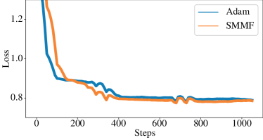
Figure 4: The loss graph of LLaMA-2-7B with LoRA fine-tuned on Alpaca dataset during the 1000 steps. The blue line indicates the Adam’s performance and the oriange line indicates the SMMF’s performance.

Figure 4 shows the loss graph of LLaMA-2-7B (Touvron et al. 2023b) fine-tuned on Alpaca (Taori et al. 2023) with LoRA (Hu et al. 2021) during the 1160 steps. Adam (Kingma and Ba 2014) shows better performance (i.e., lower loss) than SMMF at the initial few steps, but SMMF shows comparable/better performance after the initial few steps with much less memory consumption.

Appendix L Training Configurations

Since there are two types of weight decay: 1) Adam (Kingma and Ba 2014) and 2) AdamW (Loshchilov and Hutter 2019), we implement the two weight decay method (Algorithms 6 and 7). In this training configurations, we follow the weight decay method of Adam (Algorithm 6). As default schedulers for $\beta_{1,t}$ and $\beta_{2,t}$, we use the Algorithm 8. The scheduler for $\beta_{1,t}$ is from AdamNC (Kingma and Ba 2014) and the scheduler for $\beta_{2,t}$ is from Adafactor (Shazeer and Stern 2018) for stable training. The rest of tables are the training configurations using the default $beta$ schedulers. To train LLaMA-7b (Touvron et al. 2023a), we train the model using LoRA (Hu et al. 2021) with two learning-rate 5E-5 and 1E-4 which are default LoRA fine-tuning learning-rate, and choose the best result. We conduct the experiments on Ubuntu OS using PyTorch (Paszke et al. 2017) framework and NumPy (Harris et al. 2020).

Algorithm 6 Adam’s weight decay method.

 Input: Weight decay coefficient ($c$), weight parameter $\boldsymbol{W}_{t}$, and gradient $\boldsymbol{G}_{t}$ at step t.

 Take gradient $\boldsymbol{G}_{t}$

 $\boldsymbol{G}_{t}\leftarrow\boldsymbol{G}_{t}+c\times\boldsymbol{W}_{t}$

 Update momentums and weight

Algorithm 7 AdamW’s weight decay method.

 Input: Weight decay coefficient ($c$), weight parameter $\boldsymbol{W}_{t}$ at step t.

 Take gradient

 $\boldsymbol{W}_{t}\leftarrow\boldsymbol{W}_{t}-c\times\boldsymbol{W}_{t}$

 Update momentums and weight

Algorithm 8 The default schedulers for $\beta_{1,t}$ and $\beta_{2,t}$

 Input: Current step $t$, $1^{st}$ momentum coefficient $\beta_{1}$, $1^{st}$ momentum growth rate $\lambda$, $2^{nd}$ momentum decay- rate $\gamma$. The recommended growth rate is 0.999 and the decay-rate is -0.5 for CNN models (stable learning) and -0.8 for Transformer based models (better performance)

 $\beta_{1t}=\beta_{1}\lambda^{t-1}$

 $\beta_{2t}=1-t^{\gamma}$

Training Configurations of MobileNetV2 and ResNet50 on CIFAR100
Using Adam, Adafactor, SM3, CAME, and SMMF
Model	Configurations	Adam	Adafactor	SM3	CAME	SMMF
	epochs	200	200	200	200	200
	batch size	128	128	128	128	128
	warmup-steps	100	x	100	100	100
	learning-rate	0.001	x	0.001	0.001	0.001
	weight-decay	0.0005	0.0005	0.0005	0.0005	0.0005
	$\beta_{1}$	0.9	0.9	0.9	0.9	0.9
	$\beta_{2}$	0.999	x	0.999	0.999	x
	$\beta_{3}$	x	x	x	0.9999	x
	$\gamma$	x	-0.8	x	x	-0.5
	$d$	x	1	x	1	x
	$\lambda$	x	x	x	x	0.999
	$\epsilon_{1}$	1.00E-08	1.00E-30	1.00E-30	1.00E-30	1.00E-08
MobileNetV2	$\epsilon_{2}$	x	1.00E-03	x	1.00E-16	x
	epochs	200	200	200	200	200
	batch size	128	128	128	128	128
	warmup-steps	100	x	100	100	100
	learning-rate	0.001	x	0.001	0.001	0.001
	weight-decay	0.0005	0.0005	0.0005	0.0005	0.0005
	$\beta_{1}$	0.9	0.9	0.9	0.9	0.9
	$\beta_{2}$	0.999	x	0.999	0.999	x
	$\beta_{3}$	x	x	x	0.9999	x
	$\gamma$	x	-0.8	x	x	-0.5
	$d$	x	1	x	1	x
	$\lambda$	x	x	x	x	0.999
	$\epsilon_{1}$	1.00E-08	1.00E-30	1.00E-30	1.00E-30	1.00E-08
ResNet50	$\epsilon_{2}$	x	1.00E-03	x	1.00E-16	x

Table 14: The training configurations of MobileNetV2 and ResNet50 on CIFAR100 using Adam, Adafactor, SM3, CAME, and SMMF. $\lambda$ means the growth-rate, $\gamma$ means the decay-rate, $d$ means the clip-threshold. We use cosine learning-rate scheduler for 200 epochs and use an A6000 GPU.

Training Configurations of MobileNetV2 and ResNet50 on ImageNet
Using Adam, Adafactor, SM3, CAME, and SMMF
Model	Configurations	Adam	Adafactor	SM3	CAME	SMMF
	epochs	500	500	500	500	500
	batch size	128	128	128	128	128
	warmup-epochs	1	x	1	1	1
	learning-rate	0.001	x	0.001	0.001	0.001
	weight-decay	0.0005	0.0005	0.0005	0.0005	0.0005
	$\beta_{1}$	0.9	0.9	0.9	0.9	0.9
	$\beta_{2}$	0.999	x	0.999	0.999	x
	$\beta_{3}$	x	x	x	0.9999	x
	$\gamma$	x	-0.8	x	x	-0.5
	$d$	x	1	x	1	x
	$\lambda$	x	x	x	x	0.999
	$\epsilon_{1}$	1.00E-08	1.00E-30	1.00E-30	1.00E-30	1.00E-08
MobileNetV2	$\epsilon_{2}$	x	1.00E-03	x	1.00E-16	x
	epochs	500	500	500	500	500
	batch size	128	128	128	128	128
	warmup-epochs	1	x	1	1	1
	learning-rate	0.001	x	0.001	0.001	0.001
	weight-decay	0.0005	0.0005	0.0005	0.0005	0.0005
	$\beta_{1}$	0.9	0.9	0.9	0.9	0.9
	$\beta_{2}$	0.999	x	0.999	0.999	x
	$\beta_{3}$	x	x	x	0.9999	x
	$\gamma$	x	-0.8	x	x	-0.5
	$d$	x	1	x	1	x
	$\lambda$	x	x	x	x	0.999
	$\epsilon_{1}$	1.00E-08	1.00E-30	1.00E-30	1.00E-30	1.00E-08
ResNet50	$\epsilon_{2}$	x	1.00E-03	x	1.00E-16	x

Table 15: The training configurations of MobileNetV2 and ResNet50 on ImageNet using Adam, Adafactor, SM3, CAME, and SMMF. $\lambda$ means the growth-rate, $\gamma$ means the decay-rate, $d$ means the clip-threshold. We use ReduceLROnPlateau scheduler for 500 epochs and use four 3090 GPUs.

Training Configurations of YOLOv5s and YOLOv5m on COCO
Using Adam, Adafactor, SM3, CAME, and SMMF
Model	Configurations	Adam	Adafactor	SM3	CAME	SMMF
	epochs	300	300	300	300	300
	batch size	64	64	64	64	64
	warmup-epochs	3	x	3	3	3
	learning-rate0	0.001	x	0.001	0.001	0.001
	weight-decay	0.0005	0.0005	0.0005	0.0005	0.0005
	$\beta_{1}$	0.937	0.937	0.937	0.937	0.937
	$\beta_{2}$	0.999	x	0.999	0.999	x
	$\beta_{3}$	x	x	x	0.9999	x
	$\gamma$	x	-0.8	x	x	-0.5
	$d$	x	1	x	1	x
	$\lambda$	x	x	x	x	0.999
	$\epsilon_{1}$	1.00E-08	1.00E-30	1.00E-30	1.00E-30	1.00E-08
YOLOv5s	$\epsilon_{2}$	x	1.00E-03	x	1.00E-16	x
	epochs	200	200	200	200	200
	batch size	40	40	40	40	40
	warmup-epochs	3	x	3	3	3
	learning-rate0	0.001	x	0.001	0.001	0.001
	weight-decay	0.0005	0.0005	0.0005	0.0005	0.0005
	$\beta_{1}$	0.937	0.937	0.937	0.937	0.937
	$\beta_{2}$	0.999	x	0.999	0.999	x
	$\beta_{3}$	x	x	x	0.9999	x
	$\gamma$	x	-0.8	x	x	-0.8
	$d$	x	1	x	1	x
	$\lambda$	x	x	x	x	0.99
	$\epsilon_{1}$	1.00E-08	1.00E-30	1.00E-30	1.00E-30	1.00E-08
YOLOv5m	$\epsilon_{2}$	x	1.00E-03	x	1.00E-16	x

Table 16: The training configurations of YOLOv5s and YOLOv5m on COCO using Adam, Adafactor, SM3, CAME, and SMMF. $\lambda$ means the growth-rate, $\gamma$ means the decay-rate, $d$ means the clip-threshold. We use recommended configurations in YOLOv5 official code and an A6000 GPU.

Full-Training Configurations of Transformer-base and big on WMT32k
Using Adam, Adafactor, SM3, CAME, and SMMF
Model	Configurations	Adam	Adafactor	SM3	CAME	SMMF
	epochs	400	400	400	400	400
	batch size	4096	4096	4096	4096	4096
	warmup-steps	16000	x	16000	16000	16000
	weight-decay	0	0	0	0	0
	$\beta_{1}$	0.9	0.9	0.9	0.9	0.9
	$\beta_{2}$	0.997	x	0.997	0.997	x
	$\beta_{3}$	x	x	x	0.9999	x
	$\gamma$	x	-0.8	x	x	-0.5
	$d$	x	1	x	1	x
	$\lambda$	x	x	x	x	0.999
	$\epsilon_{1}$	1.00E-08	1.00E-30	1.00E-30	1.00E-30	1.00E-08
	$\epsilon_{2}$	x	1.00E-03	x	1.00E-16	x
Transformer-base	label-smoothing	0.1	0.1	0.1	0.1	0.1
	epochs	400	400	400	400	400
	batch size	4096	4096	4096	4096	4096
	warmup-steps	16000	x	16000	16000	16000
	weight-decay	0	0	0	0	0
	$\beta_{1}$	0.9	0.9	0.9	0.9	0.9
	$\beta_{2}$	0.997	x	0.997	0.997	x
	$\beta_{3}$	x	x	x	0.9999	x
	$\gamma$	x	-0.8	x	x	-0.5
	$d$	x	1	x	1	x
	$\lambda$	x	x	x	x	0.999
	$\epsilon_{1}$	1.00E-08	1.00E-30	1.00E-30	1.00E-30	1.00E-08
	$\epsilon_{2}$	x	1.00E-03	x	1.00E-16	x
Transformer-big	label-smoothing	0.1	0.1	0.1	0.1	0.1

Table 17: The full-training configurations of Transformer-base and big on WMT32k using Adam, Adafactor, SM3, CAME, and SMMF. $\lambda$ means the growth-rate, $\gamma$ means the decay-rate, $d$ means the clip-threshold. We use an A6000 GPU.

Pre-Training Configurations of BERT, GPT-2, and T5 on BookCorpus & Wikipedia-EN
Using Adam, Adafactor, SM3, CAME and SMMF
Model	Configurations	Adam	Adafactor	SM3	CAME	SMMF
	scheduler	linear
	iterations	1,000,000	1,000,000	1,000,000	1,000,000	1,000,000
	micro-batch size	4	4	4	4	4
	global-batch size	32	32	32	32	32
	warmup-steps	10,000	10,000	10,000	10,000	10,000
	learning-rate	0.0001	0.0001	0.0001	0.0001	0.0001
	weight-decay	0.01	0.01	0.01	0.01	0.01
	$\beta_{1}$	0.9	0.9	0.9	0.9	0.9
	$\beta_{2}$	0.999	x	0.999	0.999	x
	$\beta_{3}$	x	x	x	0.9999	x
	$\gamma$	x	-0.8	x	x	-0.5
	$d$	x	1	x	1	x
	$\lambda$	x	x	x	x	0.999
	$\epsilon_{1}$	1.00E-08	1.00E-30	1.00E-30	1.00E-30	1.00E-08
BERT	$\epsilon_{2}$	x	1.00E-03	x	1.00E-16	x
	scheduler	cosine
	iterations	500,000	500,000	500,000	500,000	500,000
	micro-batch size	4	4	4	4	4
	global-batch size	64	64	64	64	64
	warmup-steps	5000	5000	5000	5000	5000
	learning-rate	0.00015	0.00015	0.00015	0.00015	0.00015
	weight-decay	0.01	0.01	0.01	0.01	0.01
	$\beta_{1}$	0.9	0.9	0.9	0.9	0.9
	$\beta_{2}$	0.999	x	0.999	0.999	x
	$\beta_{3}$	x	x	x	0.9999	x
	$\gamma$	x	-0.8	x	x	-0.5
	$d$	x	1	x	1	x
	$\lambda$	x	x	x	x	0.999
	$\epsilon_{1}$	1.00E-08	1.00E-30	1.00E-30	1.00E-30	1.00E-08
GPT-2	$\epsilon_{2}$	x	1.00E-03	x	1.00E-16	x
	scheduler	linear
	iterations	1,000,000	1,000,000	1,000,000	1,000,000	1,000,000
	micro-batch size	16	16	16	16	16
	global-batch size	128	128	128	128	128
	warmup-steps	10,000	10,000	10,000	10,000	10,000
	learning-rate	0.0001	0.0001	0.0001	0.0001	0.0001
	weight-decay	0.01	0.01	0.01	0.01	0.01
	$\beta_{1}$	0.9	0.9	0.9	0.9	0.9
	$\beta_{2}$	0.999	x	0.999	0.999	x
	$\beta_{3}$	x	x	x	0.9999	x
	$\gamma$	x	-0.8	x	x	-0.5
	$d$	x	1	x	1	x
	$\lambda$	x	x	x	x	0.999
	$\epsilon_{1}$	1.00E-08	1.00E-30	1.00E-30	1.00E-30	1.00E-08
T5	$\epsilon_{2}$	x	1.00E-03	x	1.00E-16	x

Table 18: The pre-training configurations of BERT, GPT2 and T5 on BookCorpus & Wikipedia-EN using Adam, Adafactor, SM3, CAME, and SMMF. $\lambda$ means the growth-rate, $\gamma$ means the decay-rate, $d$ means the clip-threshold. We use four A6000 GPUs to train BERT, four 3090 GPUs to train T5, and four A100 to train GPT-2. We also use NVIDIA Megatron-LM code. In this task, we use low-precision weight parameter used in the Megatron-LM code.

Fine-tuning Configurations of BERT, GPT-2, and T5-small on QNLI
Using Adam, Adafactor, SM3, CAME, and SCMF
Model	Configurations	Adam	Adafactor	SM3	CAME	SMMF
	scheduler	linear
	epochs	50	50	50	50	50
	batch size	128	128	128	128	128
	warmup-steps	10	10	10	10	10
	learning-rate	2.00E-05	2.00E-05	2.00E-05	2.00E-05	2.00E-05
	weight-decay	0.0005	0.0005	0.0005	0.0005	0.0005
	$\beta_{1}$	0.9	0.9	0.9	0.9	0.9
	$\beta_{2}$	0.999	x	0.999	0.999	x
	$\beta_{3}$	x	x	x	0.9999	x
	$\gamma$	x	-0.8	x	x	-0.8
	$d$	x	1	x	1	x
	$\lambda$	x	x	x	x	0.999
	$\epsilon_{1}$	1.00E-08	1.00E-30	1.00E-30	1.00E-30	1.00E-08
BERT	$\epsilon_{2}$	x	1.00E-03	x	1.00E-16	x
	scheduler	linear
	epochs	50	50	50	50	50
	batch size	128	128	128	128	128
	warmup-steps	100	100	100	100	100
	learning-rate	2.00E-05	2.00E-05	2.00E-05	2.00E-05	2.00E-05
	weight-decay	0.0005	0.0005	0.0005	0.0005	0.0005
	$\beta_{1}$	0.9	0.9	0.9	0.9	0.9
	$\beta_{2}$	0.999	x	0.999	0.999	x
	$\beta_{3}$	x	x	x	0.9999	x
	$\gamma$	x	-0.8	x	x	-0.8
	$d$	x	1	x	1	x
	$\lambda$	x	x	x	x	0.999
	$\epsilon_{1}$	1.00E-08	1.00E-30	1.00E-30	1.00E-30	1.00E-08
GPT2	$\epsilon_{2}$	x	1.00E-03	x	1.00E-16	x
	scheduler	linear
	epochs	50	50	50	50	50
	batch size	128	128	128	128	128
	warmup-steps	100	100	100	100	100
	learning-rate	2.00E-05	2.00E-05	2.00E-05	2.00E-05	2.00E-05
	weight-decay	0.0005	0.0005	0.0005	0.0005	0.0005
	$\beta_{1}$	0.9	0.9	0.9	0.9	0.9
	$\beta_{2}$	0.999	x	0.999	0.999	x
	$\beta_{3}$	x	x	x	0.9999	x
	$\gamma$	x	-0.8	x	x	-0.8
	$d$	x	1	x	1	x
	$\lambda$	x	x	x	x	0.999
	$\epsilon_{1}$	1.00E-08	1.00E-30	1.00E-30	1.00E-30	1.00E-08
T5 (small)	$\epsilon_{2}$	x	1.00E-03	x	1.00E-16	x

Table 19: The fine-tuning configurations of BERT, GPT-2, and T5-small on QNLI using Adam, Adafactor, SM3, CAME, and SMMF. $\lambda$ means the growth-rate, $\gamma$ means the decay-rate, $d$ means the clip-threshold. We use a 3090 GPU. We use Hugging Face’s BERT (https://huggingface.co/bert-base-uncased), GPT-2 (https://huggingface.co/gpt2), and T5-small (https://huggingface.co/t5-small).

Fine-tuning Configurations of BERT, GPT-2, and T5-small on MNLI
Using Adam, Adafactor, SM3, CAME, and SCMF
Model	Configurations	Adam	Adafactor	SM3	CAME	SMMF
	scheduler	linear
	epochs	50	50	50	50	50
	batch size	128	128	128	128	128
	warmup-steps	100	100	100	100	100
	learning-rate	2.00E-05	2.00E-05	2.00E-05	2.00E-05	2.00E-05
	weight-decay	0.0005	0.0005	0.0005	0.0005	0.0005
	$\beta_{1}$	0.9	0.9	0.9	0.9	0.9
	$\beta_{2}$	0.999	x	0.999	0.999	x
	$\beta_{3}$	x	x	x	0.9999	x
	$\gamma$	x	-0.8	x	x	-0.8
	$d$	x	1	x	1	x
	$\lambda$	x	x	x	x	0.999
	$\epsilon_{1}$	1.00E-08	1.00E-30	1.00E-30	1.00E-30	1.00E-08
BERT	$\epsilon_{2}$	x	1.00E-03	x	1.00E-16	x
	scheduler	linear
	epochs	50	50	50	50	50
	batch size	128	128	128	128	128
	warmup-steps	100	100	100	100	100
	learning-rate	2.00E-05	2.00E-05	2.00E-05	2.00E-05	2.00E-05
	weight-decay	0.0005	0.0005	0.0005	0.0005	0.0005
	$\beta_{1}$	0.9	0.9	0.9	0.9	0.9
	$\beta_{2}$	0.999	x	0.999	0.999	x
	$\beta_{3}$	x	x	x	0.9999	x
	$\gamma$	x	-0.8	x	x	-0.8
	$d$	x	1	x	1	x
	$\lambda$	x	x	x	x	0.999
	$\epsilon_{1}$	1.00E-08	1.00E-30	1.00E-30	1.00E-30	1.00E-08
GPT2	$\epsilon_{2}$	x	1.00E-03	x	1.00E-16	x
	scheduler	linear
	epochs	50	50	50	50	50
	batch size	128	128	128	128	128
	warmup-steps	100	100	100	100	100
	learning-rate	2.00E-05	2.00E-05	2.00E-05	2.00E-05	2.00E-05
	weight-decay	0.0005	0.0005	0.0005	0.0005	0.0005
	$\beta_{1}$	0.9	0.9	0.9	0.9	0.9
	$\beta_{2}$	0.999	x	0.999	0.999	x
	$\beta_{3}$	x	x	x	0.9999	x
	$\gamma$	x	-0.8	x	x	-0.8
	$d$	x	1	x	1	x
	$\lambda$	x	x	x	x	0.999
	$\epsilon_{1}$	1.00E-08	1.00E-30	1.00E-30	1.00E-30	1.00E-08
T5 (small)	$\epsilon_{2}$	x	1.00E-03	x	1.00E-16	x

Table 20: The fine-tuning configurations of BERT, GPT-2, and T5-small on MNLI using Adam, Adafactor, SM3, CAME, and SMMF. $\lambda$ means the growth-rate, $\gamma$ means the decay-rate, $d$ means the clip-threshold. We use a 3090 GPU. We use Hugging Face’s BERT (https://huggingface.co/bert-base-uncased), GPT-2 (https://huggingface.co/gpt2), and T5-small (https://huggingface.co/t5-small).

Fine-tuning Configurations of BERT, GPT-2, and T5-small on QQP
Using Adam, Adafactor, SM3, CAME, and SCMF
Model	Configurations	Adam	Adafactor	SM3	CAME	SMMF
	scheduler	linear
	epochs	50	50	50	50	50
	batch size	128	128	128	128	128
	warmup-steps	100	100	100	100	100
	learning-rate	2.00E-05	2.00E-05	2.00E-05	2.00E-05	2.00E-05
	weight-decay	0.0005	0.0005	0.0005	0.0005	0.0005
	$\beta_{1}$	0.9	0.9	0.9	0.9	0.9
	$\beta_{2}$	0.999	x	0.999	0.999	x
	$\beta_{3}$	x	x	x	0.9999	x
	$\gamma$	x	-0.8	x	x	-0.8
	$d$	x	1	x	1	x
	$\lambda$	x	x	x	x	0.999
	$\epsilon_{1}$	1.00E-08	1.00E-30	1.00E-30	1.00E-30	1.00E-08
BERT	$\epsilon_{2}$	x	1.00E-03	x	1.00E-16	x
	scheduler	linear
	epochs	50	50	50	50	50
	batch size	128	128	128	128	128
	warmup-steps	100	100	100	100	100
	learning-rate	2.00E-05	2.00E-05	2.00E-05	2.00E-05	2.00E-05
	weight-decay	0.0005	0.0005	0.0005	0.0005	0.0005
	$\beta_{1}$	0.9	0.9	0.9	0.9	0.9
	$\beta_{2}$	0.999	x	0.999	0.999	x
	$\beta_{3}$	x	x	x	0.9999	x
	$\gamma$	x	-0.8	x	x	-0.8
	$d$	x	1	x	1	x
	$\lambda$	x	x	x	x	0.999
	$\epsilon_{1}$	1.00E-08	1.00E-30	1.00E-30	1.00E-30	1.00E-08
GPT2	$\epsilon_{2}$	x	1.00E-03	x	1.00E-16	x
	scheduler	linear
	epochs	50	50	50	50	50
	batch size	128	128	128	128	128
	warmup-steps	100	100	100	100	100
	learning-rate	2.00E-05	2.00E-05	2.00E-05	2.00E-05	2.00E-05
	weight-decay	0.0005	0.0005	0.0005	0.0005	0.0005
	$\beta_{1}$	0.9	0.9	0.9	0.9	0.9
	$\beta_{2}$	0.999	x	0.999	0.999	x
	$\beta_{3}$	x	x	x	0.9999	x
	$\gamma$	x	-0.8	x	x	-0.8
	$d$	x	1	x	1	x
	$\lambda$	x	x	x	x	0.999
	$\epsilon_{1}$	1.00E-08	1.00E-30	1.00E-30	1.00E-30	1.00E-08
T5 (small)	$\epsilon_{2}$	x	1.00E-03	x	1.00E-16	x

Table 21: The fine-tuning configurations of BERT, GPT-2, and T5-small on QQP using Adam, Adafactor, SM3, CAME, and SMMF. $\lambda$ means the growth-rate, $\gamma$ means the decay-rate, $d$ means the clip-threshold. We use a 3090 GPU. We use Hugging Face’s BERT (https://huggingface.co/bert-base-uncased), GPT-2 (https://huggingface.co/gpt2), and T5-small (https://huggingface.co/t5-small).

Fine-tuning Configurations of BERT, GPT-2, and T5-small on STSB
Using Adam, Adafactor, SM3, CAME, and SCMF
Model	Configurations	Adam	Adafactor	SM3	CAME	SMMF
	scheduler	linear
	epochs	50	50	50	50	50
	batch size	128	128	128	128	128
	warmup-steps	100	100	100	100	100
	learning-rate	2.00E-05	2.00E-05	2.00E-05	2.00E-05	2.00E-05
	weight-decay	0.0005	0.0005	0.0005	0.0005	0.0005
	$\beta_{1}$	0.9	0.9	0.9	0.9	0.9
	$\beta_{2}$	0.999	x	0.999	0.999	x
	$\beta_{3}$	x	x	x	0.9999	x
	$\gamma$	x	-0.8	x	x	-0.8
	$d$	x	1	x	1	x
	$\lambda$	x	x	x	x	0.999
	$\epsilon_{1}$	1.00E-08	1.00E-30	1.00E-30	1.00E-30	1.00E-08
BERT	$\epsilon_{2}$	x	1.00E-03	x	1.00E-16	x
	scheduler	linear
	epochs	50	50	50	50	50
	batch size	128	128	128	128	128
	warmup-steps	100	100	100	100	100
	learning-rate	2.00E-05	2.00E-05	2.00E-05	2.00E-05	2.00E-05
	weight-decay	0.0005	0.0005	0.0005	0.0005	0.0005
	$\beta_{1}$	0.9	0.9	0.9	0.9	0.9
	$\beta_{2}$	0.999	x	0.999	0.999	x
	$\beta_{3}$	x	x	x	0.9999	x
	$\gamma$	x	-0.8	x	x	-0.8
	$d$	x	1	x	1	x
	$\lambda$	x	x	x	x	0.999
	$\epsilon_{1}$	1.00E-08	1.00E-30	1.00E-30	1.00E-30	1.00E-08
GPT2	$\epsilon_{2}$	x	1.00E-03	x	1.00E-16	x
	scheduler	linear
	epochs	50	50	50	50	50
	batch size	128	128	128	128	128
	warmup-steps	100	100	100	100	100
	learning-rate	2.00E-05	2.00E-05	2.00E-05	2.00E-05	2.00E-05
	weight-decay	0.0005	0.0005	0.0005	0.0005	0.0005
	$\beta_{1}$	0.9	0.9	0.9	0.9	0.9
	$\beta_{2}$	0.999	x	0.999	0.999	x
	$\beta_{3}$	x	x	x	0.9999	x
	$\gamma$	x	-0.8	x	x	-0.8
	$d$	x	1	x	1	x
	$\lambda$	x	x	x	x	0.999
	$\epsilon_{1}$	1.00E-08	1.00E-30	1.00E-30	1.00E-30	1.00E-08
T5 (small)	$\epsilon_{2}$	x	1.00E-03	x	1.00E-16	x

Table 22: The fine-tuning configurations of BERT, GPT-2, and T5-small on STSB using Adam, Adafactor, SM3, CAME, and SMMF. $\lambda$ means the growth-rate, $\gamma$ means the decay-rate, $d$ means the clip-threshold. We use a 3090 GPU. We use Hugging Face’s BERT (https://huggingface.co/bert-base-uncased), GPT-2 (https://huggingface.co/gpt2), and T5-small (https://huggingface.co/t5-small).

Fine-tuning Configurations of BERT, GPT-2, and T5-small on MRPC
Using Adam, Adafactor, SM3, CAME, and SCMF
Model	Configurations	Adam	Adafactor	SM3	CAME	SMMF
	scheduler	linear
	epochs	50	50	50	50	50
	batch size	128	128	128	128	128
	warmup-steps	100	100	100	100	100
	learning-rate	2.00E-05	2.00E-05	2.00E-05	2.00E-05	2.00E-05
	weight-decay	0.0005	0.0005	0.0005	0.0005	0.0005
	$\beta_{1}$	0.9	0.9	0.9	0.9	0.9
	$\beta_{2}$	0.999	x	0.999	0.999	x
	$\beta_{3}$	x	x	x	0.9999	x
	$\gamma$	x	-0.8	x	x	-0.8
	$d$	x	1	x	1	x
	$\lambda$	x	x	x	x	0.999
	$\epsilon_{1}$	1.00E-08	1.00E-30	1.00E-30	1.00E-30	1.00E-08
BERT	$\epsilon_{2}$	x	1.00E-03	x	1.00E-16	x
	scheduler	linear
	epochs	50	50	50	50	50
	batch size	128	128	128	128	128
	warmup-steps	100	100	100	100	100
	learning-rate	2.00E-05	2.00E-05	2.00E-05	2.00E-05	2.00E-05
	weight-decay	0.0005	0.0005	0.0005	0.0005	0.0005
	$\beta_{1}$	0.9	0.9	0.9	0.9	0.9
	$\beta_{2}$	0.999	x	0.999	0.999	x
	$\beta_{3}$	x	x	x	0.9999	x
	$\gamma$	x	-0.8	x	x	-0.8
	$d$	x	1	x	1	x
	$\lambda$	x	x	x	x	0.999
	$\epsilon_{1}$	1.00E-08	1.00E-30	1.00E-30	1.00E-30	1.00E-08
GPT2	$\epsilon_{2}$	x	1.00E-03	x	1.00E-16	x
	scheduler	linear
	epochs	50	50	50	50	50
	batch size	128	128	128	128	128
	warmup-steps	100	100	100	100	100
	learning-rate	2.00E-05	2.00E-05	2.00E-05	2.00E-05	2.00E-05
	weight-decay	0.0005	0.0005	0.0005	0.0005	0.0005
	$\beta_{1}$	0.9	0.9	0.9	0.9	0.9
	$\beta_{2}$	0.999	x	0.999	0.999	x
	$\beta_{3}$	x	x	x	0.9999	x
	$\gamma$	x	-0.8	x	x	-0.8
	$d$	x	1	x	1	x
	$\lambda$	x	x	x	x	0.999
	$\epsilon_{1}$	1.00E-08	1.00E-30	1.00E-30	1.00E-30	1.00E-08
T5 (small)	$\epsilon_{2}$	x	1.00E-03	x	1.00E-16	x

Table 23: The fine-tuning configurations of BERT, GPT-2, and T5-small on MRPC using Adam, Adafactor, SM3, CAME, and SMMF. $\lambda$ means the growth-rate, $\gamma$ means the decay-rate, $d$ means the clip-threshold. We use a 3090 GPU. We use Hugging Face’s BERT (https://huggingface.co/bert-base-uncased), GPT-2 (https://huggingface.co/gpt2), and T5-small (https://huggingface.co/t5-small).

Fine-tuning Configurations of BERT and GPT-2 on SQuAD
Using Adam, Adafactor, SM3, CAME, and SCMF
Model	Configurations	Adam	Adafactor	SM3	CAME	SMMF
	scheduler	linear
	epochs	2	2	2	2	2
	batch size	12	12	12	12	12
	warmup-steps	0	0	0	0	0
	learning-rate	1.00E-05	1.00E-05	2.5E-03	1.00E-05	1.00E-05
	weight-decay	0.0	0.0	0.0	0.0	0.0
	$\beta_{1}$	0.9	0.9	0.9	0.9	0.9
	$\beta_{2}$	0.999	x	0.999	0.999	x
	$\beta_{3}$	x	x	x	0.9999	x
	$\gamma$	x	-0.8	x	x	-0.5
	$d$	x	1	x	1	x
	$\lambda$	x	x	x	x	0.999
	$\epsilon_{1}$	1.00E-08	1.00E-30	1.00E-30	1.00E-30	1.00E-08
BERT	$\epsilon_{2}$	x	1.00E-03	x	1.00E-16	x
	scheduler	linear
	epochs	2	2	2	2	2
	batch size	12	12	12	12	12
	warmup-steps	0	0	0	0	0
	learning-rate	3.00E-04	3.00E-04	2.50E-03	1.00E-05	3.00E-04
	weight-decay	0.0	0.0	0.0	0.0	0.0
	$\beta_{1}$	0.9	0.9	0.9	0.9	0.9
	$\beta_{2}$	0.999	x	0.999	0.999	x
	$\beta_{3}$	x	x	x	0.9999	x
	$\gamma$	x	-0.8	x	x	-0.5
	$d$	x	1	x	1	x
	$\lambda$	x	x	x	x	0.999
	$\epsilon_{1}$	1.00E-08	1.00E-30	1.00E-30	1.00E-30	1.00E-08
GPT2	$\epsilon_{2}$	x	1.00E-03	x	1.00E-16	x

Table 24: The fine-tuning configurations of BERT and GPT-2 on SQuAD using Adam, Adafactor, SM3, CAME, and SMMF. $\lambda$ means the growth-rate, $\gamma$ means the decay-rate, $d$ means the clip-threshold. We use a A6000 GPU. We use Hugging Face’s BERT (https://huggingface.co/bert-base-uncased) and GPT-2 (https://huggingface.co/gpt2).

Fine-tuning Configurations of T5-small on SQuADv2
Using Adam, Adafactor, SM3, CAME, and SCMF
Model	Configurations	Adam	Adafactor	SM3	CAME	SMMF
	scheduler	linear
	epochs	2	2	2	2	2
	batch size	12	12	12	12	12
	warmup-steps	0	0	0	0	0
	learning-rate	3.00E-04	3.00E-04	2.50E-03	1.00E-05	3.00E-04
	weight-decay	0.0	0.0	0.0	0.0	0.0
	$\beta_{1}$	0.9	0.9	0.9	0.9	0.9
	$\beta_{2}$	0.999	x	0.999	0.999	x
	$\beta_{3}$	x	x	x	0.9999	x
	$\gamma$	x	-0.8	x	x	-0.5
	$d$	x	1	x	1	x
	$\lambda$	x	x	x	x	0.999
	$\epsilon_{1}$	1.00E-08	1.00E-30	1.00E-30	1.00E-30	1.00E-08
T5 (small)	$\epsilon_{2}$	x	1.00E-03	x	1.00E-16	x

Table 25: The fine-tuning configurations of T5-small on SQuADv2 using Adam, Adafactor, SM3, CAME, and SMMF. $\lambda$ means the growth-rate, $\gamma$ means the decay-rate, $d$ means the clip-threshold. We use a A6000 GPU. We use Hugging Face’s T5-small (https://huggingface.co/t5-small).

Appendix M Code

We implement SMMF using PyTorch framework at github. Here is the code:

⬇

1import torch

2from typing import Optional

3

4class SMMF(torch.optim.Optimizer):

5 def __init__(

6 self, params, lr:float=1e-3, beta:Optional[float]=0.9, eps:float=1e-8, weight_decay:float=0.0,

7 decay_rate:float=-0.5, growth_rate:Optional[float]=0.999, vector_reshape:bool=True, weight_decay_mode=’adamw’

8 ):

9 if not (0.0 <= lr):

10 raise ValueError(f’Learning-rate should be greater than or equal to 0.0. Current: {lr}’)

11 if beta != None:

12 if not (0.0 <= beta and beta <= 1.0):

13 raise ValueError(f’Beta should be in [0.0, 1.0]. Current: {beta}’)

14 if not (0.0 <= eps):

15 raise ValueError(f’Epilson should be greater than or equal to 0.0. Current: {eps}’)

16 if not (0.0 <= weight_decay):

17 raise ValueError(f’Weight-decay should be greater than or equal to 0.0. Current: {weight_decay}’)

18 if not (-1.0 <= decay_rate and decay_rate <= 0.0):

19 raise ValueError(f’Decay-rate should be in [-1.0, 0.0]. Current: {decay_rate}’)

20 if not (0.0 <= growth_rate and growth_rate <= 1.0):

21 raise ValueError(f’Growth-rate should be in [0.0, 1.0]. Current: {growth_rate}’)

22

23 if (beta == None) and (growth_rate != None):

24 Warning("Beta is not used, but growth_rate is defined.")

25 defaults = dict(

26 lr=lr, beta=beta, eps=eps, weight_decay=weight_decay,

27 decay_rate=decay_rate, growth_rate=growth_rate, vector_reshape=vector_reshape

28 )

29 super(SMMF, self).__init__(params, defaults)

30 self.weight_decay_mode = weight_decay_mode

31

32 @torch.no_grad()

33 def step(self, closure=None):

34 ’’’Implements SMMF Algorithm.

35 Args:

36 params (iterable): Iterable of parameters to optimize or dicts defining parameter groups

37 lr: Learning-rate (default: 1e-3)

38 beta: Coefficient used for computing running average of gradient (default: 0.9)

39 eps: Regularization constant for square gradient (default: 1e-8)

40 weight_decay: Weight-decay (default: 0.0)

41 decay_rate: Decay-rate coefficient used for computing running average of gradient (default: -0.8)

42 growth_rate: Growth-rate coefficient used for computing running average of square gradient (default: 0.999)

43 vector_reshape: Vector Square-Matricization (default: True)

44 ’’’

45 loss = None

46 if closure is not None:

47 with torch.enable_grad():

48 loss = closure()

49

50 for group in self.param_groups:

51 for params in group[’params’]:

52 grad = params.grad

53 if grad is None:

54 continue

55

56 if group[’weight_decay’] != 0.0 and self.weight_decay_mode == ’adam’:

57 grad = grad.add(params, alpha=group[’weight_decay’])

58 elif group[’weight_decay’] != 0.0 and self.weight_decay_mode == ’adamw’:

59 params.mul_(1 - group[’lr’] * group[’weight_decay’])

60

61 dimension = len(grad.squeeze().shape)

62 factorization = not (dimension == 1 and (not group[’vector_reshape’]))

63

64 if factorization:

65 update = self._factorized_adam(params, group)

66 else:

67 update = self._adam(params, group)

68

69 params.add_(update, alpha=-group[’lr’])

70 return loss

71

72 @torch.no_grad()

73 def _factorized_adam(self, params, group):

74 beta = group[’beta’]

75 eps = group[’eps’]

76 decay_rate = group[’decay_rate’]

77 growth_rate = group[’growth_rate’]

78

79 grad = params.grad

80 state = self.state[params]

81 original_shape = grad.shape

82 device = grad.device

83

84 if len(state) == 0:

85 state[’step’] = 1

86 state[’effective_shape’] = self._get_effective_shape(params.numel())

87 if beta != None:

88 state[’momentum_m’] = (

89 torch.zeros(state[’effective_shape’][0], device=device),

90 torch.zeros(state[’effective_shape’][1], device=device),

91 )

92 state[’sign’] = torch.zeros(state[’effective_shape’], dtype=torch.bool, device=device)

93 state[’momentum_v’] = (

94 torch.zeros(state[’effective_shape’][0], device=device),

95 torch.zeros(state[’effective_shape’][1], device=device),

96 )

97

98 if not grad.is_contiguous():

99 grad = grad.contiguous()

100 grad = grad.view(state[’effective_shape’])

101

102 # Decompressing

103 if beta != None:

104 update_m = self._decompression(state, ’momentum_m’)

105 update_v = self._decompression(state, ’momentum_v’)

106

107 # Update

108 if beta != None:

109 beta_m = beta * growth_rate ** (state[’step’] - 1.0)

110 update_m.mul_(beta_m).add_(grad, alpha=(1.0 - beta_m))

111 beta_v = 1.0 - state[’step’] ** decay_rate

112 update_v.mul_(beta_v).add_(grad ** 2, alpha=(1.0 - beta_v))

113

114 # Compressing

115 if beta != None:

116 self._compression(update_m, state, ’momentum_m’)

117 self._compression(update_v, state, ’momentum_v’)

118

119 # Compute and Reshape

120 if beta != None:

121 update = update_m / (update_v.sqrt() + eps)

122 else:

123 update = grad / (update_v.sqrt() + eps)

124 update = update.contiguous().view(original_shape)

125

126 state[’step’] += 1.0

127 return update

128

129 @torch.no_grad()

130 def _adam(self, params, group):

131 beta = group[’beta’]

132 eps = group[’eps’]

133 decay_rate = group[’decay_rate’]

134 growth_rate = group[’growth_rate’]

135

136 grad = params.grad

137 state = self.state[params]

138

139 if len(state) == 0:

140 state[’step’] = 1

141 if beta != None:

142 state[’momentum_m’] = torch.zeros_like(params)

143 state[’momentum_v’] = torch.zeros_like(params)

144

145 if beta != None:

146 update_m = state[’momentum_m’]

147 update_v = state[’momentum_v’]

148

149 if beta != None:

150 beta_m = beta * growth_rate ** (state[’step’] - 1.0)

151 update_m.mul_(beta_m).add_(grad, alpha=(1.0 - beta_m))

152 beta_v = 1.0 - state[’step’] ** decay_rate

153 update_v.mul_(beta_v).add_(grad ** 2, alpha=(1.0 - beta_v))

154

155 if beta != None:

156 state[’momentum_m’] = update_m

157 state[’momentum_v’] = update_v

158

159 if beta != None:

160 update = update_m / (update_v.sqrt() + eps)

161 else:

162 update = grad / (update_v.sqrt() + eps)

163

164 state[’step’] += 1.0

165 return update

166

167 @torch.no_grad()

168 def _get_effective_shape(self, numel:int)->tuple:

169 sqrt_num = int(numel ** 0.5) ** 2

170

171 if numel == sqrt_num:

172 sqrt_num = int(numel ** 0.5)

173 return (sqrt_num, sqrt_num)

174

175 reversed_range = reversed(range(1, int(numel **0.5) + 1))

176 for i in reversed_range:

177 if numel % i == 0:

178 return (numel // i, i)

179

180 return (numel, 1)

181

182 @torch.no_grad()

183 def _decompression(self, state, momentum:str)->torch.Tensor:

184 update = self._unnmf(state[momentum])

185 if momentum == ’momentum_m’:

186 sign = state[’sign’]

187 if sign.dtype != torch.bool:

188 sign = sign.type(torch.bool)

189 torch.where(sign, update, -update, out=update)

190 return update

191

192 @torch.no_grad()

193 def _compression(self, matrix:torch.Tensor, state, momentum:str)->tuple:

194 if momentum == ’momentum_m’:

195 state[’sign’] = matrix > 0

196 self._nnmf(torch.abs(matrix), out=state[momentum] )

197 else:

198 self._nnmf(matrix, out=state[momentum])

199 return state[momentum]

200

201 @torch.no_grad()

202 def _unnmf(self, row_col:tuple)->torch.Tensor:

203 return torch.outer(row_col[0], row_col[1])

204

205 @torch.no_grad()

206 def _nnmf(self, matrix:torch.Tensor, out)->tuple:

207 shape = matrix.shape

208 torch.sum(matrix, dim=1, out=out[0])

209 torch.sum(matrix, dim=0, out=out[1])

210

211 if shape[0] < shape[1]:

212 scale = out[0].sum()

213 if scale != 0:

214 torch.div(out[0], scale, out=out[0])

215 else:

216 scale = out[1].sum()

217 if scale != 0:

218 torch.div(out[1], scale, out=out[1])

219

220 return out

References

- Abdulkadirov, Lyakhov, and Nagornov (2023) Abdulkadirov, R.; Lyakhov, P.; and Nagornov, N. 2023. Survey of Optimization Algorithms in Modern Neural Networks. Mathematics, 11(11): 2466.
- Aghajanyan, Zettlemoyer, and Gupta (2020) Aghajanyan, A.; Zettlemoyer, L.; and Gupta, S. 2020. Intrinsic Dimensionality Explains the Effectiveness of Language Model Fine-Tuning. arXiv:2012.13255.
- Amari (2010) Amari, S.-i. 2010. Information geometry in optimization, machine learning and statistical inference. Frontiers of Electrical and Electronic Engineering in China, 5: 241–260.
- Anil et al. (2019) Anil, R.; Gupta, V.; Koren, T.; and Singer, Y. 2019. Memory Efficient Adaptive Optimization. In Wallach, H.; Larochelle, H.; Beygelzimer, A.; d'Alché-Buc, F.; Fox, E.; and Garnett, R., eds., Advances in Neural Information Processing Systems, volume 32. Curran Associates, Inc.
- Bojar et al. (2014) Bojar, O.; Buck, C.; Federmann, C.; Haddow, B.; Koehn, P.; Leveling, J.; Monz, C.; Pecina, P.; Post, M.; Saint-Amand, H.; et al. 2014. Findings of the 2014 workshop on statistical machine translation. In Proceedings of the ninth workshop on statistical machine translation, 12–58.
- Bojar et al. (2016) Bojar, O. r.; Chatterjee, R.; Federmann, C.; Graham, Y.; Haddow, B.; Huck, M.; Jimeno Yepes, A.; Koehn, P.; Logacheva, V.; Monz, C.; Negri, M.; Neveol, A.; Neves, M.; Popel, M.; Post, M.; Rubino, R.; Scarton, C.; Specia, L.; Turchi, M.; Verspoor, K.; and Zampieri, M. 2016. Findings of the 2016 Conference on Machine Translation. In Proceedings of the First Conference on Machine Translation, 131–198. Berlin, Germany: Association for Computational Linguistics.
- Chen et al. (2016) Chen, T.; Xu, B.; Zhang, C.; and Guestrin, C. 2016. Training deep nets with sublinear memory cost. arXiv preprint arXiv:1604.06174.
- Devlin et al. (2018) Devlin, J.; Chang, M.-W.; Lee, K.; and Toutanova, K. 2018. Bert: Pre-training of deep bidirectional transformers for language understanding. arXiv preprint arXiv:1810.04805.
- Dong et al. (2020) Dong, K.; Zhou, C.; Ruan, Y.; and Li, Y. 2020. MobileNetV2 Model for Image Classification. In 2020 2nd International Conference on Information Technology and Computer Application (ITCA), 476–480.
- Finesso and Spreij (2006) Finesso, L.; and Spreij, P. 2006. Nonnegative matrix factorization and I-divergence alternating minimization. Linear Algebra and its Applications, 416(2): 270–287.
- Google (2022) Google. 2022. Coral Dev Board Micro. Https://coral.ai/products/dev-board-micro/.
- Harris et al. (2020) Harris, C. R.; Millman, K. J.; van der Walt, S. J.; Gommers, R.; Virtanen, P.; Cournapeau, D.; Wieser, E.; Taylor, J.; Berg, S.; Smith, N. J.; Kern, R.; Picus, M.; Hoyer, S.; van Kerkwijk, M. H.; Brett, M.; Haldane, A.; del Río, J. F.; Wiebe, M.; Peterson, P.; Gérard-Marchant, P.; Sheppard, K.; Reddy, T.; Weckesser, W.; Abbasi, H.; Gohlke, C.; and Oliphant, T. E. 2020. Array programming with NumPy. Nature, 585(7825): 357–362.
- He et al. (2016) He, K.; Zhang, X.; Ren, S.; and Sun, J. 2016. Deep Residual Learning for Image Recognition. In 2016 IEEE Conference on Computer Vision and Pattern Recognition (CVPR), 770–778.
- Hinton, Srivastava, and Swersky (2012) Hinton, G.; Srivastava, N.; and Swersky, K. 2012. Neural networks for machine learning lecture 6a overview of mini-batch gradient descent. Cited on, 14(8): 2.
- Hu et al. (2021) Hu, E. J.; Shen, Y.; Wallis, P.; Allen-Zhu, Z.; Li, Y.; Wang, S.; Wang, L.; and Chen, W. 2021. LoRA: Low-Rank Adaptation of Large Language Models. arXiv:2106.09685.
- Kingma and Ba (2014) Kingma, D. P.; and Ba, J. 2014. Adam: A method for stochastic optimization. arXiv preprint arXiv:1412.6980.
- Krizhevsky, Hinton et al. (2009) Krizhevsky, A.; Hinton, G.; et al. 2009. Learning multiple layers of features from tiny images.
- Kumar et al. (2019) Kumar, R.; Panigrahy, R.; Rahimi, A.; and Woodruff, D. 2019. Faster Algorithms for Binary Matrix Factorization. In Chaudhuri, K.; and Salakhutdinov, R., eds., Proceedings of the 36th International Conference on Machine Learning, volume 97 of Proceedings of Machine Learning Research, 3551–3559. PMLR.
- Lan et al. (2020) Lan, Z.; Chen, M.; Goodman, S.; Gimpel, K.; Sharma, P.; and Soricut, R. 2020. ALBERT: A Lite BERT for Self-supervised Learning of Language Representations. arXiv:1909.11942.
- Landro et al. (2022a) Landro, N.; Gallo, I.; La Grassa, R.; and Federici, E. 2022a. Two New Datasets for Italian-Language Abstractive Text Summarization. Information, 13(5).
- Landro et al. (2022b) Landro, N.; Gallo, I.; La Grassa, R.; and Federici, E. 2022b. Two New Datasets for Italian-Language Abstractive Text Summarization. Information, 13(5).
- Lee and Seung (1999) Lee, D. D.; and Seung, H. S. 1999. Learning the parts of objects by non-negative matrix factorization. Nature, 401(6755): 788–791.
- Lewis et al. (2019) Lewis, M.; Liu, Y.; Goyal, N.; Ghazvininejad, M.; Mohamed, A.; Levy, O.; Stoyanov, V.; and Zettlemoyer, L. 2019. BART: Denoising Sequence-to-Sequence Pre-training for Natural Language Generation, Translation, and Comprehension. arXiv:1910.13461.
- Li et al. (2018) Li, C.; Farkhoor, H.; Liu, R.; and Yosinski, J. 2018. Measuring the Intrinsic Dimension of Objective Landscapes. arXiv:1804.08838.
- Lin et al. (2015) Lin, T.-Y.; Maire, M.; Belongie, S.; Bourdev, L.; Girshick, R.; Hays, J.; Perona, P.; Ramanan, D.; Zitnick, C. L.; and Dollár, P. 2015. Microsoft COCO: Common Objects in Context. arXiv:1405.0312.
- Liu and Nocedal (1989) Liu, D. C.; and Nocedal, J. 1989. On the limited memory BFGS method for large scale optimization. Mathematical programming, 45(1-3): 503–528.
- Liu et al. (2020) Liu, Y.; Gu, J.; Goyal, N.; Li, X.; Edunov, S.; Ghazvininejad, M.; Lewis, M.; and Zettlemoyer, L. 2020. Multilingual Denoising Pre-training for Neural Machine Translation. arXiv:2001.08210.
- Liu et al. (2019) Liu, Y.; Ott, M.; Goyal, N.; Du, J.; Joshi, M.; Chen, D.; Levy, O.; Lewis, M.; Zettlemoyer, L.; and Stoyanov, V. 2019. RoBERTa: A Robustly Optimized BERT Pretraining Approach. arXiv:1907.11692.
- Loshchilov and Hutter (2019) Loshchilov, I.; and Hutter, F. 2019. Decoupled Weight Decay Regularization. arXiv:1711.05101.
- Luo et al. (2023) Luo, Y.; Ren, X.; Zheng, Z.; Jiang, Z.; Jiang, X.; and You, Y. 2023. CAME: Confidence-guided Adaptive Memory Efficient Optimization. In Rogers, A.; Boyd-Graber, J.; and Okazaki, N., eds., Proceedings of the 61st Annual Meeting of the Association for Computational Linguistics (Volume 1: Long Papers), 4442–4453. Toronto, Canada: Association for Computational Linguistics.
- Martens (2016) Martens, J. 2016. Second-order optimization for neural networks. University of Toronto (Canada).
- Nallapati et al. (2016) Nallapati, R.; Zhou, B.; dos santos, C. N.; Gulcehre, C.; and Xiang, B. 2016. Abstractive Text Summarization Using Sequence-to-Sequence RNNs and Beyond. arXiv:1602.06023.
- Narayan, Cohen, and Lapata (2018) Narayan, S.; Cohen, S. B.; and Lapata, M. 2018. Don’t Give Me the Details, Just the Summary! Topic-Aware Convolutional Neural Networks for Extreme Summarization. ArXiv, abs/1808.08745.
- OpenAI et al. (2024) OpenAI; Achiam, J.; Adler, S.; Agarwal, S.; Ahmad, L.; Akkaya, I.; Aleman, F. L.; Almeida, D.; Altenschmidt, J.; Altman, S.; Anadkat, S.; Avila, R.; Babuschkin, I.; Balaji, S.; Balcom, V.; Baltescu, P.; Bao, H.; Bavarian, M.; Belgum, J.; Bello, I.; Berdine, J.; Bernadett-Shapiro, G.; Berner, C.; Bogdonoff, L.; Boiko, O.; Boyd, M.; Brakman, A.-L.; Brockman, G.; Brooks, T.; Brundage, M.; Button, K.; Cai, T.; Campbell, R.; Cann, A.; Carey, B.; Carlson, C.; Carmichael, R.; Chan, B.; Chang, C.; Chantzis, F.; Chen, D.; Chen, S.; Chen, R.; Chen, J.; Chen, M.; Chess, B.; Cho, C.; Chu, C.; Chung, H. W.; Cummings, D.; Currier, J.; Dai, Y.; Decareaux, C.; Degry, T.; Deutsch, N.; Deville, D.; Dhar, A.; Dohan, D.; Dowling, S.; Dunning, S.; Ecoffet, A.; Eleti, A.; Eloundou, T.; Farhi, D.; Fedus, L.; Felix, N.; Fishman, S. P.; Forte, J.; Fulford, I.; Gao, L.; Georges, E.; Gibson, C.; Goel, V.; Gogineni, T.; Goh, G.; Gontijo-Lopes, R.; Gordon, J.; Grafstein, M.; Gray, S.; Greene, R.; Gross, J.; Gu, S. S.; Guo, Y.; Hallacy, C.; Han, J.; Harris, J.; He, Y.; Heaton, M.; Heidecke, J.; Hesse, C.; Hickey, A.; Hickey, W.; Hoeschele, P.; Houghton, B.; Hsu, K.; Hu, S.; Hu, X.; Huizinga, J.; Jain, S.; Jain, S.; Jang, J.; Jiang, A.; Jiang, R.; Jin, H.; Jin, D.; Jomoto, S.; Jonn, B.; Jun, H.; Kaftan, T.; Łukasz Kaiser; Kamali, A.; Kanitscheider, I.; Keskar, N. S.; Khan, T.; Kilpatrick, L.; Kim, J. W.; Kim, C.; Kim, Y.; Kirchner, J. H.; Kiros, J.; Knight, M.; Kokotajlo, D.; Łukasz Kondraciuk; Kondrich, A.; Konstantinidis, A.; Kosic, K.; Krueger, G.; Kuo, V.; Lampe, M.; Lan, I.; Lee, T.; Leike, J.; Leung, J.; Levy, D.; Li, C. M.; Lim, R.; Lin, M.; Lin, S.; Litwin, M.; Lopez, T.; Lowe, R.; Lue, P.; Makanju, A.; Malfacini, K.; Manning, S.; Markov, T.; Markovski, Y.; Martin, B.; Mayer, K.; Mayne, A.; McGrew, B.; McKinney, S. M.; McLeavey, C.; McMillan, P.; McNeil, J.; Medina, D.; Mehta, A.; Menick, J.; Metz, L.; Mishchenko, A.; Mishkin, P.; Monaco, V.; Morikawa, E.; Mossing, D.; Mu, T.; Murati, M.; Murk, O.; Mély, D.; Nair, A.; Nakano, R.; Nayak, R.; Neelakantan, A.; Ngo, R.; Noh, H.; Ouyang, L.; O’Keefe, C.; Pachocki, J.; Paino, A.; Palermo, J.; Pantuliano, A.; Parascandolo, G.; Parish, J.; Parparita, E.; Passos, A.; Pavlov, M.; Peng, A.; Perelman, A.; de Avila Belbute Peres, F.; Petrov, M.; de Oliveira Pinto, H. P.; Michael; Pokorny; Pokrass, M.; Pong, V. H.; Powell, T.; Power, A.; Power, B.; Proehl, E.; Puri, R.; Radford, A.; Rae, J.; Ramesh, A.; Raymond, C.; Real, F.; Rimbach, K.; Ross, C.; Rotsted, B.; Roussez, H.; Ryder, N.; Saltarelli, M.; Sanders, T.; Santurkar, S.; Sastry, G.; Schmidt, H.; Schnurr, D.; Schulman, J.; Selsam, D.; Sheppard, K.; Sherbakov, T.; Shieh, J.; Shoker, S.; Shyam, P.; Sidor, S.; Sigler, E.; Simens, M.; Sitkin, J.; Slama, K.; Sohl, I.; Sokolowsky, B.; Song, Y.; Staudacher, N.; Such, F. P.; Summers, N.; Sutskever, I.; Tang, J.; Tezak, N.; Thompson, M. B.; Tillet, P.; Tootoonchian, A.; Tseng, E.; Tuggle, P.; Turley, N.; Tworek, J.; Uribe, J. F. C.; Vallone, A.; Vijayvergiya, A.; Voss, C.; Wainwright, C.; Wang, J. J.; Wang, A.; Wang, B.; Ward, J.; Wei, J.; Weinmann, C.; Welihinda, A.; Welinder, P.; Weng, J.; Weng, L.; Wiethoff, M.; Willner, D.; Winter, C.; Wolrich, S.; Wong, H.; Workman, L.; Wu, S.; Wu, J.; Wu, M.; Xiao, K.; Xu, T.; Yoo, S.; Yu, K.; Yuan, Q.; Zaremba, W.; Zellers, R.; Zhang, C.; Zhang, M.; Zhao, S.; Zheng, T.; Zhuang, J.; Zhuk, W.; and Zoph, B. 2024. GPT-4 Technical Report. arXiv:2303.08774.
- Paszke et al. (2017) Paszke, A.; Gross, S.; Chintala, S.; Chanan, G.; Yang, E.; DeVito, Z.; Lin, Z.; Desmaison, A.; Antiga, L.; and Lerer, A. 2017. Automatic Differentiation in PyTorch. In NIPS 2017 Workshop on Autodiff.
- Radford et al. (2019) Radford, A.; Wu, J.; Child, R.; Luan, D.; Amodei, D.; Sutskever, I.; et al. 2019. Language models are unsupervised multitask learners. OpenAI blog, 1(8): 9.
- Raffel et al. (2020) Raffel, C.; Shazeer, N.; Roberts, A.; Lee, K.; Narang, S.; Matena, M.; Zhou, Y.; Li, W.; and Liu, P. J. 2020. Exploring the limits of transfer learning with a unified text-to-text transformer. The Journal of Machine Learning Research, 21(1): 5485–5551.
- Rajpurkar, Jia, and Liang (2018) Rajpurkar, P.; Jia, R.; and Liang, P. 2018. Know What You Don’t Know: Unanswerable Questions for SQuAD. arXiv:1806.03822.
- Rajpurkar et al. (2016) Rajpurkar, P.; Zhang, J.; Lopyrev, K.; and Liang, P. 2016. SQuAD: 100,000+ Questions for Machine Comprehension of Text. arXiv:1606.05250.