Efficient Reinforcement Learning for Optimal Control with Natural Images

Abstract

Reinforcement learning solves optimal control and sequential decision problems widely found in control systems engineering, robotics, and artificial intelligence. This work investigates optimal control over a sequence of natural images. The problem is formalized, and general conditions are derived for an image to be sufficient for implementing an optimal policy. Reinforcement learning is shown to be efficient only for certain types of image representations. This is demonstrated by developing a reinforcement learning benchmark that scales easily with number of states and length of horizon, and has optimal policies that are easily distinguished from suboptimal policies. Image representations given by overcomplete sparse codes are found to be computationally efficient for optimal control, using fewer computational resources to learn and evaluate optimal policies. For natural images of fixed size, representing each image as an overcomplete sparse code in a linear network is shown to increase network storage capacity by orders of magnitude beyond that possible for any complete code, allowing larger tasks with many more states to be solved. Sparse codes can be generated by devices with low energy requirements and low computational overhead.

Keywords Natural image sequences  $\cdot$ Overcomplete sparse codes  $\cdot$ Optimal policies  $\cdot$ Sufficient statistics

1 Introduction

Many interesting and complex tasks can be described using natural image sequences. Each image of the sequence corresponds to a particular state of the environment, and choosing an action or applying a control at the current state takes the environment to its next state, and leads to the next image in the sequence. A natural question is then: given an image, what is the best control to apply? Although the answer will depend on the particular task at hand a general framework can be identified. As a simple example, consider moving through a rainforest and taking images of flowers in order to locate a particular species of plant. In this case, each image describes a state of the environment, and the state changes depending on the location of the next image. Each image also has a cost or reward associated with it: an image of the sought-after flower will receive a high reward, while an image without any flowers may receive a low (or even negative) reward. To perform this task well, the choice of control leading to the location of the next image does not necessarily give the best chance of obtaining an image of the sought-after flower at the next time period, rather, it should also lead to a good chance of obtaining such images at future time periods as you move through the rainforest. Planning over a sequence of time periods is the defining characteristic of sequential decision problems and optimal control, and is clearly a requirement of any intelligent system.

Natural images are a high-dimensional dataset with a great deal of expressive power. For some tasks, images may include enough task-dependent information to determine an optimal policy. In this case an image is similar to a belief state in a partially observed Markov decision process, and we will derive the general conditions for an image to be sufficient for implementing an optimal policy. Similar to other types of ecological data, it is well-known that the statistical properties of natural images distinguish them from artificially generated images (Field, 1987, 1994; Ruderman and Bialek, 1994; Ruderman, 1997; Simoncelli and Olshausen, 2001; Hyvärinen et al., 2009; Hosseini et al., 2010). We exploit these statistical properties to find efficient image representations that significantly decrease the computational resources required for finding optimal policies.

The aim of this work is to develop a general framework for the efficient solution of Markov decision processes and optimal control tasks involving natural image sequences. This includes developing a new reinforcement learning benchmark for comparing the performance and efficiency of different image representations. The benchmark must be scalable so the number of states and time periods can easily be increased; and optimal solutions must easily be distinguishable from suboptimal solutions. Scalability of the benchmark is necessary for determining which image representations will perform best over long horizons and for large numbers of states.

Most reinforcement learning is done with synthetic data of limited complexity, and previous work in this area has suggested that more work should be done to extend the paradigm of reinforcement learning to real-world data such as natural images and natural video (Zhang et al., 2018). Past examples of these efforts include using image representations to integrate unsupervised training of deep neural networks into reinforcement learning; specifically for visual navigation (Lange and Riedmiller, 2010), and simulated autonomous driving tasks (Zhang et al., 2021). In order to obtain better policies with neural networks on standard classic control tasks, previous work has also investigated the use of sparse coding and sparse representations in reinforcement learning (Le et al., 2017; Liu et al., 2018; Rafati and Noelle, 2019). Although none of these works considered images or other high-dimensional datasets, and computational efficiency was not investigated. The closest previous work to that presented here is in Loxley (2021), where sparse image representations were shown to significantly decrease the computational resources required for finding optimal policies. However, this work was limited by a small video dataset, which meant that extending results to large numbers of states and long horizons was not possible. Further, only a deterministic optimal control task was considered rather than a general Markov decision process, and the overcomplete sparse representations investigated were very small. In this work, a more general approach to optimal control is taken, and the development of a new reinforcement learning benchmark allows results for image representations to be significantly scaled up by orders of magnitude.

In this work, natural images are represented as overcomplete sparse codes. Statistical dependencies in natural images lead to redundancy, making it possible to obtain an efficient representation using an appropriate encoding scheme such as sparse coding (Daugman, 1988, 1989; Olshausen and Field, 1996, 1997). A sparse code is efficient in the sense of being a low bit-rate (low entropy) representation of a high-dimensional dataset. As shown here, an overcomplete sparse code also turns out to be computationally efficient for finding optimal policies in reinforcement learning. A sparse code for natural images can be generated in many different ways – from simple constructions using multiresolution wavelet bases and autoencoders (Daugman, 1988; Loxley, 2017, 2021), through to heavy-duty approaches that apply deep neural networks (Papyan et al., 2017; Li et al., 2024). The ICA algorithm (Bell and Sejnowski, 1997; Hyvärinen et al., 2009) is another well-know method for generating sparse codes; however, it cannot be applied here as it does not generate overcomplete sparse codes, which are key to this work. Sparse codes may also be generated directly from hardware using purpose built low-power neuromorphic computer chips (Fair et al., 2019).

The structure of this paper is as follows. In Sec. 2, the reinforcement learning methodology is briefly summarized, and the problem of optimal control over a sequence of natural images is formalized. Following this, a new reinforcement learning benchmark is developed step by step. In Sec. 3, results for the reinforcement learning benchmark are presented, and different image representations are compared. A detailed discussion of results and conclusions is given in Sec. 4.

2 Reinforcement Learning over Natural Image Sequences

Consider a general optimal control task involving a discrete-time dynamical system with a finite number of states and controls (Bertsekas, 2017, 2019). During any time period $k$ the environment is described by a state $i_{k}$ taken from a state-space $S_{k}$, and a control $u_{k}$ is selected from a set of available controls $U_{k}(i_{k})\subset C_{k}$. The state of the environment changes when a controller chooses control $u$ during the current time period, so that state $i$ updates to the successor state $j$ according to the transition probabilities $p_{ij}(u)$ of a controllable Markov chain. The controller can choose different controls depending on the current state of the environment as well as the time period under consideration: the controller’s choice is then described by a policy $\pi=\{\mu_{0},...,\mu_{N-1}\}$, which is a sequence of functions $\mu_{k}$ that map states into controls: $\mu_{k}(i_{k})=u_{k}$, for each state $i_{k}$ at each time period $k$. The cost of being in state $i_{k}$ at time period $k$, choosing control $u_{k}$, then moving to state $i_{k+1}$, is denoted by $g_{k}(i_{k},u_{k},i_{k+1})$. The key quantity of interest is the expected total cost. Given a policy $\pi$ and an initial state $i_{0}$, the expected total cost is the expected value of the sum of costs:

$$J_{\pi}(i_{0})={\mathbb{E}}\left\{g_{N}(i_{N})+\sum_{k=0}^{N-1}g_{k}(i_{k},\mu_{k}(i_{k}),i_{k+1})\right\},$$ (1)

where $g_{N}(i_{N})$ is the terminal cost incurred at the end of the task ($k=N$); and the expectation is taken over the states $i_{1},...,i_{N-1}$ using the transition probabilities $p_{ij}(\mu_{k}(i))$, the initial state $i_{0}$, and the chosen policy $\pi=\{\mu_{0},...,\mu_{N-1}\}$. The goal of optimal control is to choose a policy so as to minimize the expected total cost; i.e.,

$$\text{minimize}\ \ \ J_{\pi}(i_{0}),$$ (2)

$$\text{subject to}\ \ \ \mu_{k}(i)\in U_{k}(i)\ \ \ \ \ \ \forall k,i.$$

The finite-horizon optimal control task outlined in Eqs. (1) and (2) can be solved exactly using the Dynamic Programming Algorithm, leading to the optimal cost-to-go $J_{k}^{*}$ (this algorithm is called Value Iteration in the case of infinite horizon tasks, and converges to $J^{*}$ for discounted problems with stationary policies). The optimal policy $\mu_{k}^{*}(i)$ can then be found from the following minimization:

$$\underset{u\in U_{k}(i)}{\operatorname{min}}\ \sum_{j}p_{ij}(u)\left(g_{k}(i,u,j)+J_{k+1}^{*}(j)\right),$$ (3)

by choosing the minimizing control $u^{*}$ in Eq. (3) for each state $i$ and each time period $k$.

Optimal control over natural image sequences has additional issues to address; such as how to represent natural images as states, what information to include in a state to allow for optimal decision-making, and how to include natural images into optimal control algorithms. In the simplest case, each state $i_{k}\in S_{k}$ in an optimal control task becomes a natural image $\phi_{k}(i)\in S_{k}^{\prime}$; where $S_{k}^{\prime}\subset\mathbb{R}^{p}$ so that each image is represented as a $p$-dimensional vector. The cost-to-go can then be described using a parametric function approximator $\bar{J}_{k}(\phi_{k}(i),r_{k})$ that approximates the optimal cost-to-go $J_{k}^{*}$. This can be done by using a neural network architecture that accepts images $\phi_{k}(i)$ as input, and adjusting the network parameters $r_{k}\in\mathbb{R}^{p}$ (called “weights”) to approximate $J_{k}^{*}$ by $\bar{J}_{k}$. When neural network training includes all states at each time period and the neural network is below its memory capacity, $\bar{J}_{k}$ may provide an accurate description of $J_{k}^{*}$. The optimal policy $\mu_{k}^{*}(i)$ can then be found from the following minimization:

$$\underset{u\in U_{k}(i)}{\operatorname{min}}\ \sum_{j}p_{ij}(u)\left(g_{k}(i,u,j)+\bar{J}_{k+1}(\phi_{k+1}(j),r_{k+1}^{*})\right),$$ (4)

by choosing the minimizing control $u^{*}$ in expression (4) for each state $i$ and each time period $k$.

A key issue to address is what information to include in a state. Any state that includes all necessary information for optimal control is called a sufficient statistic (Bertsekas, 2017). A natural image $\phi_{k}$ is a sufficient statistic, provided $U_{k}(i),p_{ij}(u)$, and $g_{k}(i,u,j)$ in Eq. (4) depend on $i$ or $j$ only through $\phi_{k}(i)$ or $\phi_{k+1}(j)$, respectively. The optimal policy can then be written as

$$\mu_{k}^{*}(i)=\bar{\mu}_{k}(\phi_{k}(i)),$$ (5)

where $\bar{\mu}_{k}$ is some appropriate function. The most striking consequence of $\phi_{k}$ as a sufficient statistic is the form the transition probabilities now take:

$$p_{ij}(u)=\bar{p}(\phi_{k+1}(j)|\phi_{k}(i),u),$$ (6)

so that given a current image $\phi_{k}(i)$, selecting control $u$ leads to a new image $\phi_{k+1}(j)$ at the next time period (with some probability). Therefore, the transition probabilities describe an “image generator”. We derive a simple image generator in the next section.

To approximate the optimal cost-to-go $J_{k}^{*}(i)$ using $\bar{J}_{k}(\phi_{k}(i),r_{k})$, the weights $r_{k}$ can be found using Fitted Value Iteration. To start the iteration, we go to the end of the task at $k=N-1$, and make use of the known terminal cost $\bar{J}_{N}(\phi_{N}(i),r_{N})=g_{N}(i)$. The following pair of expressions are then evaluated to yield $\bar{J}_{N-1}(\phi_{N-1}(i),r_{N-1})$:

$$\beta_{k}^{i}=\underset{u\in U_{k}(i)}{\operatorname{min}}\ \sum_{j}p_{ij}(u)\left(g_{k}(i,u,j)+\bar{J}_{k+1}(\phi_{k+1}(j),r_{k+1})\right),\ \ \ \ \ \forall i\in S_{k}$$ (7)

$$\text{minimize}\ \ \ \sum_{i\in S_{k}}(\bar{J}_{k}(\phi_{k}(i),r_{k})-\beta_{k}^{i})^{2},$$ (8)

$$\text{subject to}\ \ \ r_{k}\in\mathbb{R}^{p}.$$

This process is continued by iterating backwards from $k=N-2$ to $k=0$, yielding the cost-to-goes $\bar{J}_{N-2},...,\bar{J}_{0}$ required in (4) for finding an optimal policy. The first expression (7) performs the minimization given in Eq. (4) for each of the states using the parametric function $\bar{J}_{k+1}(\phi_{k+1}(j),r_{k+1})$ for the cost-to-go of image $\phi_{k+1}(j)$ at time period $k+1$. This results in the cost-to-go $\beta_{k}^{i}$ for image $\phi_{k}(i)$ at time period $k$. In the second expression (8), the state and cost-to-go pair $(i,\beta_{k}^{i})$ from Eq. (7) is used to fit the parametric function $\bar{J}_{k}(\phi_{k}(i),r_{k})$ to the cost-to-go of image $\phi_{k}(i)$ at time period $k$ by adjusting the weights $r_{k}$ to minimize the sum of squares.

2.1 A Scalable Benchmark for Efficient Image Representations

We would now like to design a simple and robust benchmark for the purpose of assessing alternative image representations for reinforcement learning with natural image sequences. The number of states of the benchmark should scale to arbitrarily large numbers, its cost structure should be simple and easy to implement over long horizons, and its transition probabilities should correspond to a natural image generator that is easy to implement.

The number of states of the benchmark can scale to arbitrarily large numbers by working with image patches. Image patches are arbitrarily-sized image regions extracted from a larger parent image. Discretizing the $k$th parent image into a regular grid pattern yields a set of image patches $S_{k}^{\prime}$, with each image patch denoted by $\phi_{k}(i)$; where $i\in\mathbb{Z}^{2}$ is a unique pair of coordinates giving the location of the image patch within its parent image (for example, each coordinate pair could give the coordinates of the top-left corner of an image patch). The number of image patches can be increased by decreasing the size of each image patch, similar to the case of discretizing a continuous variable where decreasing the step size increases the number of steps. The following proposition then shows the number of states of the benchmark is scalable.

Proposition 1.

A state of the benchmark can be described by $i_{k}$ or $\phi_{k}(i)$, and either state is a sufficient statistic.

Proof.

Given any image patch $\phi_{k}(i)\in S_{k}^{\prime}$, it is possible to determine state $i\in S_{k}$ as

$$\hat{i}=\underset{m}{\operatorname{argmin}}\lVert\phi_{k}(m)-\phi_{k}(i)\rVert_{2}^{2},$$

provided each image patch is unique. Alternatively, given state $i$, it is possible to determine state $\phi_{k}(i)$ by looking up the $i$th element of $S_{k}^{\prime}=\{\phi_{k}(1),...,\phi_{k}(n)\}$. The same is true for both $\phi_{k+1}(j)\in S_{k+1}^{\prime}$ and $j\in S_{k+1}$. Therefore, given $p_{ij}(u)$, $g_{k}(i,u,j)$, and $U_{k}(i)$; it is possible to determine $\bar{p}(\phi_{k+1}(j)|\phi_{k}(i),u)=p_{ij}(u)$, $\bar{g}_{k}(\phi_{k}(i),u,\phi_{k+1}(j))=g_{k}(i,u,j)$, and $\bar{U}_{k}(\phi_{k}(i))=U_{k}(i)$. Alternatively, given $\bar{p}(\phi_{k+1}(j)|\phi_{k}(i),u)$, $\bar{g}_{k}(\phi_{k}(i),u,\phi_{k+1}(j))$, and $\bar{U}_{k}(\phi_{k}(i))$; it is possible to determine $p_{ij}(u)=\bar{p}(\phi_{k+1}(j)|\phi_{k}(i),u)$, $g_{k}(i,u,j)=\bar{g}_{k}(\phi_{k}(i),u,\phi_{k+1}(j))$, and $U_{k}(i)=\bar{U}_{k}(\phi_{k}(i))$. But this means $i$ or $\phi_{k}(i)$ is sufficient for determining $u$ from the minimization in Eq. (4). ∎

The proof of Proposition 1 describes a very simple natural image generator $\bar{p}(\phi_{k+1}(j)|\phi_{k}(i),u)$ constructed from the transition probabilities $p_{ij}(u)$ and the image patch set $S_{k}^{\prime}$. A non-trivial model for $p_{ij}(u)$ is presented in the next sections.

The cost structure and transition probabilities of the benchmark are motivated by dragonfly tracking in videos (Loxley, 2021). The tracking task requires a tracker to follow a target as closely as possible over many time periods using a set of discrete controls that determines the dynamics of the tracker (see Fig. 1). Letting the image patch coordinates be related to the distance between the tracker and target allows this distance to be used to assign a cost to each image patch at each time period. Moving from one image patch to another changes this distance, and therefore the cost. An optimal policy corresponds to the optimal choice of controls for tracking the target starting from any image patch during any time period. This task is easily scalable to long horizons and many states provided the target dynamics scales well. Next, a scalable model for the target dynamics is presented.

2.1.1 Target Dynamics

The target dynamics for the benchmark has two key requirements: 1) the target must be difficult enough to track so that simple algorithms such as greedy search perform suboptimally, and 2) the dynamics must easily scale to long horizons and many states. Both points can be addressed by introducing a simple generative model for the target dynamics.

Motivated by the dragonfly video dataset used for optimal control in Loxley (2021), the following type of scenario is proposed. The target (T) starts on the bottom row of a $3\times 3$ grid (shown in Fig 1, first grid). The target and the tracker can both move up, left, or right at each time period. However, the target (but not the tracker) can also make an “evade” move by moving diagonally to evade the tracker. The tracker must therefore carefully plan its sequence of moves to follow the target closely.

During the first time period (second grid in Fig 1) the target remains where it is, while at the beginning of the second time period (third grid in Fig 1) it makes a diagonal move. An optimal tracker (blue square) anticipates a diagonal move immediately following a time period where the target is stationary, and pays a small cost to move up one square during the first time period (second grid in Fig 1). Whether the target next moves diagonally-left or diagonally-right, the optimal tracker is now able to reach the target during the next time period (third grid in Fig 1). On the other hand, a tracker applying a greedy algorithm (red squares) tries to stay as close to the target as possible during each time period, allowing the target to “evade” the greedy tracker when it makes its diagonal move, and the greedy tracker falls one move behind the target (third and fourth grids in Fig 1). A greedy tracker will always be suboptimal for this sequence.

Figure 1: A target tracking sequence (from left to right) showing optimal and suboptimal trackers. A tracker can move either “up” or “right”, while the target can move “up”, “right”, or “diagonally”. The suboptimal tracker (red square) follows the target (T) as closely as possible at each step (a greedy approach), causing it to fall behind when the target moves diagonally. The optimal tracker (blue square) follows the target by anticipating a diagonal move following a time period where the target is stationary.

The sequence of target moves in Fig 1 can be generalized and modelled as a regular language (Sipser, 2012). The alphabet of target-moves is $\{\mathrm{s,d,r}\}$; where $\mathrm{s}\rightarrow(0,0)$, $\mathrm{d}\rightarrow(1,1)\ \text{or}\ (-1,1)$, and $\mathrm{r}\rightarrow(0,1)\ \text{or}\ (-1,0)\ \text{or}\ (1,0)$. Each symbol in the alphabet represents a change in the target coordinates, $\Delta t$, as the target moves from its current position to its next position. The regular expression given by $\mathrm{r}^{*}\cup(\mathrm{sdr})^{*}$ generates all strings in this language, representing all possible target dynamics. For example, the string given by “$\mathrm{sdr}$” represents the sequence in Fig 1: $\Delta t_{1}=(0,0)$; $\Delta t_{2}=(1,1)$; and $\Delta t_{3}=(0,1)$. According to this sequence, a target starting at $(2,1)$ stays at $(2,1)$ during the first time period; then moves to $(3,2),$ and $(3,3)$ in the second, and third time periods, respectively (see Fig 1).

A Markov chain can be constructed to generate stochastic dynamics obeying this language. To parameterize the Markov chain, we see the only degree of freedom available in the regular expression is whether a symbol of a substring begins with an “$\mathrm{r}$” or an “$\mathrm{s}$”. This can be parameterized using the probability $p$, leading to the Makov chain shown in Fig 2.

Figure 2: A Markov chain for generating the target dynamics shown in Fig 1. In Fig 1, the states $\mathrm{s,d,}$ and $\mathrm{r}$ correspond to “same position”, “diagonal move”, and “up” or “right”, respectively. The non-zero transition probabilities are: $p(\Delta t_{k}=\mathrm{d}|\Delta t_{k-1}=\mathrm{s})=1$, $p(\Delta t_{k}=\mathrm{r}|\Delta t_{k-1}=\mathrm{d})=1$, $p(\Delta t_{k}=\mathrm{s}|\Delta t_{k-1}=\mathrm{r})=1-p$, and $p(\Delta t_{k}=\mathrm{r}|\Delta t_{k-1}=\mathrm{r})=p$.

Different values of $p$ give different steady-state distributions for this Markov chain. When $p=0$ or 1, the target dynamics is a deterministic repeating sequence: $(\mathrm{sdr})^{*}$ for $p=0$, and $\mathrm{r}^{*}$ for $p=1$. When $0<p<1$, the Markov chain is recurrent and non-periodic: i.e., when $p=0.5$ the steady-state probabilities of $\mathrm{s,d,}$ and $\mathrm{r}$ are $1/4$, $1/4$, and $1/2$, respectively; and a typical sequence looks like $\mathrm{sdrrsdrrrrsdr}$.

2.1.2 Target Tracking

It is now possible to specify the reinforcement learning benchmark in terms of a target tracking task. This task requires two dynamical variables $t_{k},c_{k}\in\mathbb{Z}^{2}$ representing the discrete two-dimensional coordinates of a target, and a controller (tracker), respectively, at time period $k$. Changes to the environment are described by the discrete dynamical system:

$$t_{k+1}=t_{k}+\Delta t_{k},$$ (9)

$$c_{k+1}=c_{k}+u_{k}.$$ (10)

A target updates its position from $t_{k}$ to $t_{k+1}$ according to the transition probabilities of the Markov chain presented in Sec. 2.1.1. In order to follow the target as closely as possible a controller updates its position from $c_{k}$ to $c_{k+1}$ by choosing a control $u_{k}$ from the set $U$ of available controls. Complete state information required for choosing optimal controls is given when the state is defined to be:

$$i_{k}=(c_{k}-t_{k},\Delta t_{k-1})\in D\times T,$$ (11)

where $c_{k}-t_{k}\in D$, and $\Delta t_{k-1}\in T$; so that $S_{k}=D\times T$. Here, $D,T,U\subset\mathbb{Z}^{2}$ are finite sets of integer pairs. In order to derive the transition probabilities of the corresponding controllable Markov chain, $p_{ij}(u)$, we proceed as follows. According to Eq. (11), and making use of Eqs. (9) and (10), the state update is given by

$$i_{k+1} =(c_{k+1}-t_{k+1},\Delta t_{k}),$$

$$=(c_{k}-t_{k}+u_{k}-\Delta t_{k},\Delta t_{k}).$$ (12)

Denoting the state $i=i_{k}$ and its successor $j=i_{k+1}$ in terms of their individual components:

$$i=(a_{1},b_{1}),\ \ \ \ j=(a_{2},b_{2}),$$ (13)

and equating with Eqs. (11) and (12), then leads to $a_{1}=c_{k}-t_{k},b_{1}=\Delta t_{k-1},a_{2}=a_{1}+u_{k}-\Delta t_{k},$ and $b_{2}=\Delta t_{k}$. These equations can be viewed as constraints on the allowed values of $j$ via $a_{2}$ and $b_{2}$, and represented as $\delta(a_{2}-(a_{1}+u_{k}-\Delta t_{k}))$ and $\delta(b_{2}-\Delta t_{k})$; where $\delta(k)=1$ if $k=0$, and $\delta(k)=0$ otherwise. The controllable Markov chain is governed by the the Markov chain from Fig. 2 describing the target dynamics: $p(\Delta t_{k}|\Delta t_{k-1})$, as well as the constraints on $j$, giving:

$$p_{ij}(u) =\sum_{\Delta t_{k}}p(\Delta t_{k}|b_{1})\delta(a_{2}-(a_{1}+u-\Delta t_{k}))\delta(b_{2}-\Delta t_{k}),$$ (14)

$$=p(b_{2}|b_{1})\delta(a_{2}-(a_{1}+u-b_{2})).$$ (15)

The cost per time period is the distance between the tracker and the target at each time period, and is given by

$$g_{k}(i,u,j)=\lVert a_{1}\rVert_{2}^{2},$$ (16)

where $\lVert.\rVert_{2}$ is the Euclidean distance. An optimal policy for the benchmark can be found after substituting these choices into Expression (4), leading to:

$$\underset{u\in U}{\operatorname{min}}\ \sum_{b_{2}}p(b_{2}|b_{1})\bar{J}_{k+1}(\phi_{k+1}(a_{1}+u-b_{2},b_{2}),r_{k+1}^{*}),$$ (17)

which is evaluated at each state $(a_{1},b_{1})\in D\times T$ and each time period $k$. The final choice for the benchmark is the form of the parametric function $\bar{J}_{k}$. A simple choice is a network architecture that is linear in the weights $r_{k}$ and given by the following scalar product:

$$\bar{J}_{k}(\phi_{k}(i),r_{k})=r^{\top}_{k}\phi_{k}(i),$$ (18)

where $\top$ is the vector transpose. The Eq. (18) makes it clear that once the weights $r_{k}$ are determined through training, $\bar{J}_{k}$ depends only on the input image $\phi_{k}$.

The benchmark is now completely specified by Eqs. (17) and (18), with Eqs. (7) and (8) used for determining $r_{k}^{*}$. The advantage of set notation is that once the sets $D,T$, and $U$ are specified, all that remains is to choose an initial state $(a_{1},b_{1})\in D\times T$ and evaluate the benchmark.

Applying the target dynamics from Sec. 2.1.1 with uniform probabilities over the “or” choices results in tracking tasks that become too uncertain over time, leading to degenerate policies that preform poorly. It is therefore necessary to work with a simpler dynamics given by $\mathrm{s}=(0,0)$, $\mathrm{d}=(1,1)$, and $\mathrm{r}=(0,1)$. The sets $T$ and $U$ then become $T=\{(0,0),(1,1),(0,1)\}$ and $U=\{(0,0),(1,0),(0,1)\}$; while the set $D$ depends on the number of coordinate differences (i.e., distances) chosen between the target and the controller. Therefore, the number of states of the benchmark is determined by choice of the size of $D$.

3 Results

Results for the reinforcement learning benchmark developed in Section 2 are now presented. We begin by looking at the optimal and greedy policies for target tracking.

3.1 Optimal and Greedy Policies in the Reinforcement-Learning Benchmark

The evasive target dynamics in the benchmark leads to different policies for optimal and greedy tracking. When $p=0$ in the Markov chain, the target dynamics is deterministic and periodic and given by the repeating sequence $(\mathrm{sdr})^{*}$. The optimal policy from Eq. (17) is given in Table 1 when the chain is initially in state $\mathrm{s}$, and cycles between three states: $i_{k}=((0,1),(0,0))$, $i_{k+1}=((0,0),(1,1))$, and $i_{k+2}=((0,0),(0,1))$.

State	Control	Cost
$((0,1),(0,0))$	$(1,0)$	1
$((0,0),(1,1))$	$(0,1)$	0
$((0,0),(0,1))$	$(0,1)$	0

Table 1: Optimal policy $\mu^{*}$ and cost per time period $g$.

Only the first state has a non-zero cost, and therefore the total cost of the optimal policy increases by one every three time periods. This is shown in Fig 3 for $p=0$.

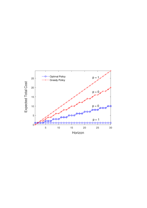
Figure 3: Expected total cost of the optimal policy from Table 1 (blue circles), and the greedy policy from Table 2 (red pluses), as the horizon goes from $N=1$ to 30 time periods for $p=0$ and $p=1$.

The greedy policy can be found by replacing $\bar{J}_{k+1}$ in Eq. (17) with $g_{k+1}$, leading to the simpler expression:

$$\underset{u^{G}\in U}{\operatorname{min}}\ \sum_{b_{2}}p(b_{2}|b_{1})\lVert a_{1}+u^{G}-b_{2}\rVert_{2}^{2}.$$ (19)

According to Eq. (19), a greedy tracker chooses $u^{G}$ as close as possible to $b_{2}-a_{1}$ (so that $c_{k+1}$ is as close as possible to $t_{k+1}$ at the next time period), without regard for what may happen at future time periods. That is, a greedy tracker has no scope for planning ahead. The greedy policy from Eq. (19) is given in Table 2.

State	Control	Cost
$((0,0),(0,0))$	$(1,0)$	0
$((0,-1),(1,1))$	$(0,1)$	1
$((0,-1),(0,1))$	$(0,1)$	1

Table 2: Greedy policy $\mu^{G}$ and cost per time period $g$.

The greedy policy also cycles between three states, with a total cost that increases by two every three time periods, as shown in Fig 3 for $p=0$. This means the greedy policy has twice the total cost of the optimal policy when $p=0$, over any number of complete cycles.

When $p=1$, the target dynamics is given by the repeating sequence $\mathrm{r}^{*}$. The optimal policy in Table 1 is now $\mu^{*}((0,0),(0,1))=(0,1)$, with cost per time period $g((0,0),(0,1))=0$. Similarly, the greedy policy in Table 2 is now $\mu^{G}((0,-1),(0,1))=(0,1)$, with cost per time period $g((0,-1),(0,1))=1$. The ratio of total costs of the greedy and optimal policies is therefore $N-1$ to 1, so the greedy policy always has a cost $N-1$ times larger than that of the optimal policy, as seen in Fig. 3 for $p=1$.

When $0<p<1$, the target dynamics is stochastic, recurrent, and non-periodic: at the next time period, state $\mathrm{r}$ has probability $p$ of staying in the same state, and probability $1-p$ of going to state $\mathrm{s}$. The expected total cost of the optimal policy in Table 1 now lies somewhere between the curves for the optimal policies with $p=1$ and $p=0$ in Fig. 3. Similarly, the expected total cost of the greedy policy in Table 2 now lies between the curves for the greedy policies with $p=0$ and $p=1$ in Fig. 3. The optimal policy and its expected total cost were found using both fitted value iteration and the dynamic programming algorithm, with both approaches yielding the same results. Results for the greedy policy were found directly from Eq. (1) with $\mu_{k}(i)=\mu_{k}^{G}(i)$ from Eq. (19) using an efficient algorithm described in the Appendix. These results were also confirmed using policy evaluation; that is, solving $J_{k}(i)=\sum_{j}p_{ij}(\mu_{k}^{G}(i))(g_{k}(i,\mu_{k}^{G}(i),j)+J_{k+1}(j))$ using dynamic programming iterations. In this case, $J_{N}(i)$ was set to the terminal cost as for fitted value iteration and dynamic programming.

3.2 Benchmark Performance with Length of Horizon

The optimal and greedy policies given in Tables 1 and 2 turn out to be stationary policies for all values of $p$. This is confirmed using an infinite horizon analysis. The cost of each policy is found in the Appendix by introducing a discount factor and applying policy evaluation in the infinite horizon limit ($N\rightarrow\infty$). These calculations are in complete agreement with value iteration applied to the discounted problem (not shown). In addition, the ratio of costs of the greedy and optimal policies in Tables 1 and 2 is given in the Appendix for the case of an infinite horizon, and the result is completely consistent with our discussion of these policies for finite horizons. For example, in the infinite horizon limit the expected total cost ratio of greedy and optimal policies becomes 2 when $p=0$, 5 when $p=0.75$, and diverges when $p=1$. For finite horizons, the first result ($p=0$) is most easily seen in Fig 3 when $N=30$; giving a ratio of $20/10=2$. The final result ($p=1$) is also seen in Fig 3 when $N=30$, giving a ratio of $29/1=29$; which will clearly diverge as $N\rightarrow\infty$. The result for $p=0.75$ can be seen from the ratio of expected total costs of the greedy and optimal results in Fig 7.

The optimal and greedy policies undergo more complicated dynamics over shorter horizons when different initial states are chosen. For an initial state given by $((0,1),(0,0))$ (i.e., where the tracker starts close to the target) the bottom pair of curves in Fig. 4 reach the stationary optimal and greedy policies in Tables 1 and 2 at very short horizons. As the initial distance between the tracker and target increases for positive coordinates (middle and top pairs of curves in Fig. 4), the optimal and greedy policies take longer and longer to reach these stationary policies. For example, the top pair of curves has not reached their stationary policies until the horizon is around 14 time periods. These results suggest the dynamics of all initial states with one positive coordinate and one non-negative coordinate eventually reach the stationary policies in Tables 1 and 2 provided the horizon is long enough.

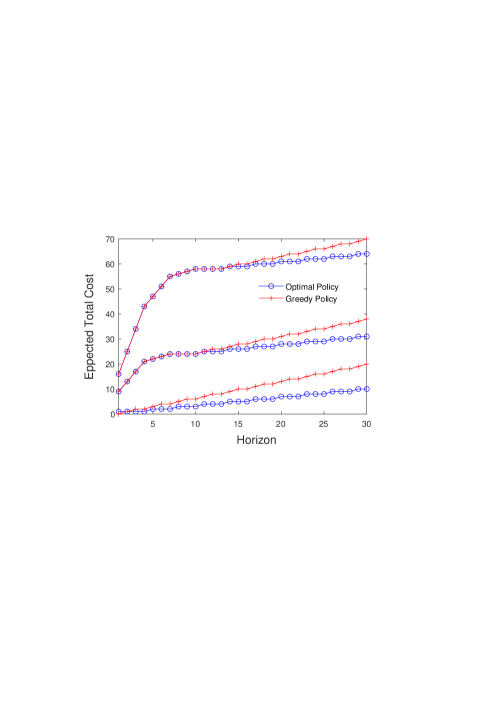
Figure 4: Expected total cost of optimal and greedy policies as the horizon goes from $N=1$ to $N=30$ time periods for $p=0$ with different initial states. The bottom pair of curves start at state $((0,1),(0,0))$; the middle pair start at state $((3,0),(0,0))$; and the top pair start at state $((4,0),(0,0))$.

In Fig. 4, the greedy policy is shown to be an optimal policy when the initial state of the tracker is far from the target. Reaching a stationary policy only happens when the tracker gets close enough to the target (within a distance of one). Once the tracker is close to the target the greedy policy is no longer optimal (as shown for longer horizons in Fig. 4). For initial states where both coordinates are negative, the tracker is always behind the target and can never catch up. A simple greedy approach is then sufficient to follow the target, ensuring that the greedy policy is an optimal policy in this case. A more detailed discussion of initial state dependence is given in Sec. 3.5.

3.3 Efficient Image Representations for Reinforcement Learning

To find efficient representations for natural image sequences used in reinforcement learning, image patches from the benchmark were transformed into overcomplete sparse codes and whitened complete codes. A set of 48 natural images was taken from the database “Natural Scene Statistics in Vision Science” by Geisler and Perry (2011). Each image was cropped to $2844\times 2844$ pixels to make it square, then converted to grayscale and double precision using the Matlab functions rgb2gray and im2double, and subsequently discretized into square image patches of side-length $a$ (in pixels). The number of image patches in a single image was $\lfloor 2844/a\rfloor^{2}$; where the function $\lfloor.\rfloor$ rounds down to the nearest integer.

Overcomplete sparse codes were constructed using the method described in Loxley (2021) and summarized in the Appendix. This method relies on the two-dimensional Gabor function, originally used to model simple-cell receptive field profiles in the primary visual cortex (Hubel and Wiesel, 1959; Jones and Palmer, 1987; Daugman, 1985, 1989). The Gabor function parameters are chosen by drawing samples from a tractable multivariate probability distribution that well-approximates natural image statistics (Loxley, 2017). A sparse code is given by the hidden-layer activities of an autoencoder with an input/output that comprises the same image patch, and connection weights given by 2D Gabor functions adapted to natural image statistics. The encoding requires solving a linear least-squares problem, while decoding is a simple matrix-vector multiplication. The size of the sparse code depends on the number of Gabor functions used to generate the code. To generate a $\times 64$ overcomplete sparse code, the number of Gabor functions required is $64\times a^{2}$ for an image patch of $a^{2}$ pixels. For reasons that will become apparent, we would like to choose $a$ to maximize the number of image patches available in a $2844\times 2844$ image, whilst ensuring the size of a $\times 64$ overcomplete sparse code is larger than this number; i.e., $64\times a^{2}>\lfloor 2844/a\rfloor^{2}$. The unique solution to this problem is $a=19$, leading to 22201 image patches of 361 pixels each.

A more traditional method of pixel decorrelation (whitening) was used to construct complete codes: where the representation has the same number of pixels as the image patch it was derived from. This method was carried out by setting the mean pixel values (taken over all image patches) to zero, and diagonalizing the corresponding covariance matrix. This method does not generalize to overcomplete codes.

3.4 Benchmark Performance with Number of States

Training a neural network on efficient image representations takes fewer computational resources than training it directly on images (Loxley, 2021). This is shown in Figs. 5 and 6, where the number of least-squares iterations required to store a given number of cost-to-go values in a linear network is shown for network inputs given by image patches and image-patch representations. Each state of the benchmark corresponds to a unique image patch and its associated cost-to-go value. By adjusting the network weights during training, this association is stored in the network in order to determine an optimal policy. In a linear network, the number of network weights determines the storage capacity of the network; that is, the maximum number of cost-to-go values it can store. In turn, the number of weights is equal to the number of pixel inputs to the network; since each input is multiplied by its corresponding weight and summed together to yield the network output. Therefore, the storage capacity of a network can be increased by increasing the number of pixel inputs and network weights. One way to do this for a fixed-sized image patch is to generate an overcomplete representation of the image patch, and use this as input to the network instead. This approach will be used to solve the benchmark tracking task as the number of states, and therefore, the number of stored cost-to-go values, increases. Network training is carried out using the Matlab lsqr function running on an Nvidia GPU, with the number of least-squares iterations until convergence (within $1\times 10^{-6}$ of the least-squares objective), averaged over 48 independent trials, shown along the vertical axis.

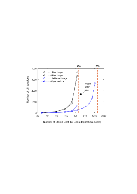
Figure 5: Number of least-squares iterations to store a number of cost-to-go values in a linear network using different image-patch representations (see legend). The least-squares objective is found within a tolerance of $1\times 10^{-6}$, and the number of iterations are averaged over 48 independent trials. Each image patch is 400 pixels.

In Fig. 5, the size of each image patch was chosen to be 400 pixels instead of 361 pixels for visualization purposes when the number of stored cost-to-goes is relatively small. When the input is either an image patch or a complete representation of an image patch, a linear network will have exactly 400 inputs and 400 weight parameters, allowing it to store a maximum of 400 cost-to-go values. The curve with black circles ($\times 1$ raw image), and the curve with blue circles ($\times 1$ whitened image) show each of these cases, and both curves get close to 400 stored cost-to-goes. However, input given by a whitened image generally takes far fewer least-squares iterations to store the same number of cost-to-goes as input given by a raw image, making it an efficient image representation. The curve with black triangles ($\times 4$ raw image) shows results for a natural image patch that has been upscaled by a factor of four using bicubic interpolation via Matlab’s imresize function, while the curve with blue triangles ($\times 4$ sparse code) shows results for an overcomplete sparse code. Each of these representations has 1600 pixels (i.e., $4\times 400$ pixels, treating Gabor coefficients in a sparse code the same as double-precision pixels in an image). Increasing the number of weights to 1600 allows a linear network to store a maximum of 1600 cost-to-go values. However, the best result for the $\times 4$ resized image remains below 400 stored cost-to-goes, and uses approximately the same number of least-squares iterations as the best result for the $\times 4$ sparse code; which gets close to 1600 stored cost-to-goes (the best result in Fig. 5 is at 1323 cost-to-goes for 2701 least-squares iterations). These results confirm that an efficient image representation must be both overcomplete and sparse in order to increase the storage capacity of a linear network. The key role of sparsity is discussed in Loxley (2021), where it is shown how a sparse code that decorrelates neighbouring pixels can lead to an increase in the column-space dimension of the design matrix for the least-squares problem.

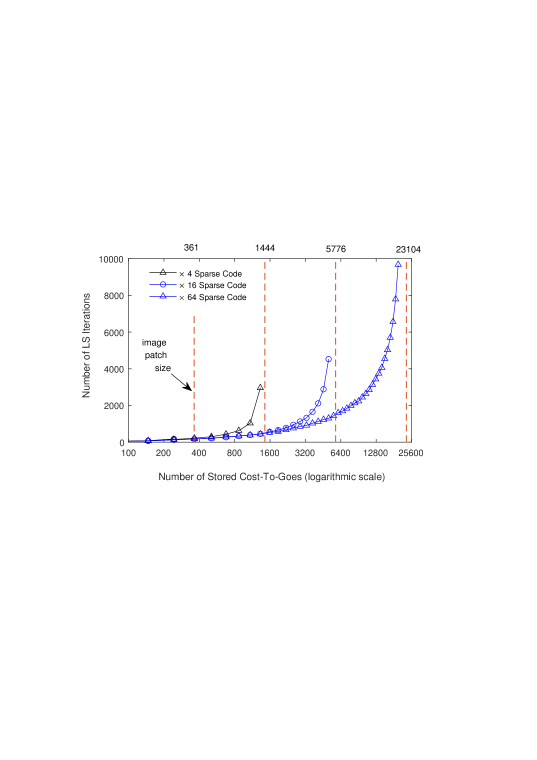
Figure 6: Number of least-squares iterations to store a number of cost-to-go values in a linear network using different image-patch representations (see legend). The least-squares objective is found within a tolerance of $1\times 10^{-6}$, and the number of iterations are averaged over 48 independent trials. Each image patch is 361 pixels.

Surprisingly, if we continue to increase the overcompleteness of image representations, the network storage capacity continues to increase. This is shown in Fig 6 for network inputs given by $\times 4$, $\times 16$, and $\times 64$ overcomplete sparse codes. The size of each image patch is 361 pixels; so the $\times 4$ sparse code has $4\times 361=1444$ pixels, the $\times 16$ sparse code has $16\times 361=5776$ pixels, and the $\times 64$ sparse code has $64\times 361=23104$ pixels. These quantities are shown as dashed vertical lines in Fig 6. The general result in Fig 6 is that the number of stored cost-to-goes (i.e., the network storage capacity) increases as the overcompleteness of an image representation increases. The first vertical dashed line at 361 cost-to-go values corresponds to the maximum storage capacity for a linear network with inputs given by complete codes. The other vertical dashed lines correspond to maximum storage capacities for inputs given by $\times 4,\ \times 16,$ and $\times 64$ overcomplete sparse codes, respectively.

The best result for each representation in Fig 6 is summarized in Table 3. An extra data point is given in Table 3 to show the limit of our calculation at 21675 stored cost-to-go values (not shown in Fig 6). This limit holds because we have a maximum of 22201 image patches, while the parameterization of the benchmark set $D$ implemented here means the next data point is a benchmark with 22707 states – more than the available number of image patches.

Representation	$\#$ LS Iterations	$\#$ Stored Cost-To-Goes
$\times 1$ whitened image	177	243
$\times 4$ sparse code	2963	1323
$\times 16$ sparse code	4527	5043
$\times 64$ sparse code	9679	19683
$\times 64$ sparse code	20009	21675

Table 3: (Top) Four data points in Fig 6. (Bottom) One data point not shown in Fig  6.

Some variation in the average number of least-squares iterations can be seen in Table 3, particularly for the $\times 4$ sparse code. This is due to the relative proximity of each data point to its limiting case given by each of the vertical dashed lines. For example, the best result for the $\times 4$ sparse code is the data point at 1323 stored cost-to-go values, which is closer to its limiting value of 1444 than any other image representation is to its limiting value, and hence requires a relatively large number of least-squares iterations as a result of the larger condition number of its Hessian matrix.

Now we are in a position to look at how the benchmark performs as the number of states increases. Increasing the number of states increases the size of the region for target tracking, and the number of stored cost-to-go values required for an optimal solution. Following from the results in Fig 6, we would expect that efficient image representations should increase the number of states over which optimal target tracking is possible. Fig 7 shows this result: the expected total cost of tracking a target with $p=0.75$ over thirty time periods is shown for various image representations as the number of states of the benchmark is increased. The initial states are $((0,1),(0,0))$ for the optimal tracker, and $((0,0),(0,0))$ for the greedy tracker. For comparison, the exact expected total costs for optimal and greedy target tracking are shown as the two right columns in Fig 7.

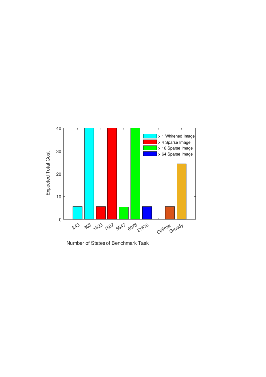
Figure 7: Expected total cost of tracking a target over 30 time periods with $p=0.75$ versus number of states of the benchmark, for different image-patch representations (see legend). Exact expected total costs for optimal and greedy target tracking (right columns) are shown for comparison.

According to Fig 7, a representation given by a $\times 1$ whitened image can solve the benchmark optimally for 243 states, but not for 363 states – where the expected total cost exceeds that for greedy target tracking. The reason is, as in Fig 6, a complete code stores a maximum of 361 cost-to-go values – which is less than 363. Similarly, a $\times 4$ sparse code can solve the benchmark optimally for 1323 states, but not for 1587 ($>1444$) states; a $\times 16$ sparse code can solve the benchmark optimally for 5547 states, but not for 6075 ($>5776$) states; and a $\times 64$ sparse code can solve the benchmark optimally for 21675 states. This number was the largest number of image patches tested in this work. Values for the numbers of states shown in Fig 7 result from the parameterization of the benchmark set $D$ implemented here, as previously mentioned.

3.5 Benchmark Performance for Different Initial States

We now look at the effect of starting at different initial states in the reinforcement learning benchmark. This is done by starting the benchmark in an initial state, and then running it with optimal and greedy policies until reaching the horizon. The total cost of the optimal and greedy policies can then be compared. This is repeated for each state of the benchmark.

Training the benchmark with a $\times 64$ sparse code leads to 21675 possible initial states. The expected total cost of optimal and greedy policies is shown in Fig 8 for each initial state leading to a suboptimal greedy policy. These initial states are indexed from 1 to 10880, comprising roughly half of the 21675 available initial states. For the remaining 10795 initial states (not shown) the greedy policy is the optimal policy. The benchmark horizon is 200 time periods, and the Markov chain parameter is $p=0.4$. The policy found using fitted value iteration exactly matches the optimal policy found using dynamic programming, as shown in Fig 8 (Inset) for initial states indexed from 4000 to 4050. Fig 9 shows the distribution of cost differences, given by the cost of the greedy policy minus the cost of the optimal policy, for each initial state in Fig 8. These cost differences increase further for longer horizons.

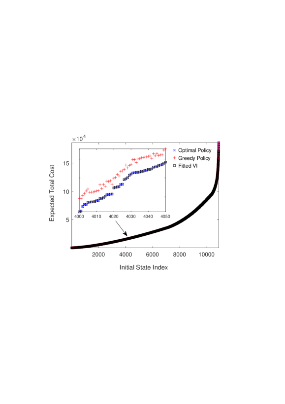
Figure 8: Expected total cost of optimal and greedy policies for each initial state leading to a suboptimal greedy policy. These initial states are indexed from 1 to 10880. Fitted VI is the policy found using fitted value iteration. Inset shows a close-up of initial states indexed from 4000 to 4050. The benchmark horizon is 200 time periods, and $p=0.4$ (see Text for details).

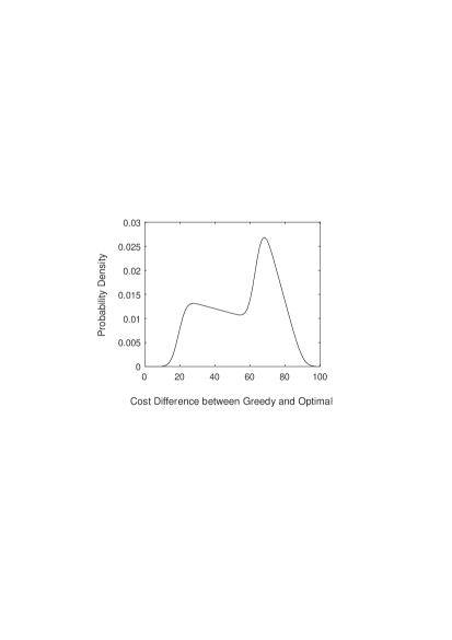
Figure 9: Fitted distribution of cost differences, given by the cost of the greedy policy minus the cost of the optimal policy, for each initial state in Fig 8. The fitted distribution is a kernel density estimate using the Gaussian distribution with bandwidth = 3.47.

Looking at a few specific initial states helps to understand Fig 8. The lowest cost optimal policy starts at state $((0,0),(1,1))$ and has an expected total cost of 54. Since this state is part of the stationary policy in Table 1, we can find its total cost for $p=0$; which is $(200-2)/3\times 1=66$. From Fig 3, we also know the optimal cost for $p=0.4$ would be less than that for $p=0$, justifying the order relation $54<66$. Further, making use of the infinite horizon result from the Appendix, we predict an approximate value for the expected total cost of the greedy policy as: $(1+1/(1-p))\times 54=144$ for $p=0.4$. This exactly matches the value in Fig 8.

Now that we have a reasonable theoretical justification for the lowest cost policy in Fig 8, let us attempt to understand the highest cost policy. This policy starts at state $((42,-42),(1,1))$ and has an expected total cost of $185870$ for the optimal policy, and $185890$ for the greedy policy. We can understand this as follows. Each coordinate for $c_{k}-t_{k}$ in the benchmark has the range $[-42,42]$ when the number of states is 21675. Starting at state $((42,-42),(1,1))$ means the tracker is very far behind the target, but it is also very far to the right of the target. Consider the corresponding situation when $p=0$: during three time periods, the target will move right once and up twice. If the tracker simply moves up three times over the same three time periods, it can reach the target within $42\times 3=126$ time periods, and apply the stationary optimal policy thereafter. There is no other initial state with a suboptimal greedy policy that can have a larger expected total cost. The same argument holds approximately when $p=0.4$.

For the remaining 10795 initial states where the greedy policy is the optimal policy, the lowest cost policy starts at state $((0,0),(0,0))$ and has an expected total cost of 145. This is close to the expected total cost of the greedy policy for the initial state $((0,0),(1,1))$ just discussed. Predictably, the highest cost policy starts with the tracker as far behind the target as possible, in state $((-42,-42),(1,1))$, and has an expected total cost of $701100$.

3.6 Benchmark Performance with Alternative Sampling Strategies

Now we consider sampling strategies where only some of the states (image patches) of the benchmark are used to train the network. One possibility would be to focus training on initial states that have a suboptimal greedy policy. However, under an optimal policy states outside this set are visited. A better approach makes use of the findings in the previous section. Sampling from states with at least one non-negative coordinate for $c_{k}-t_{k}$ in the benchmark corresponds to training on the set of states where the tracker is not both behind and to the left of the target. Many of these states are independent of the set of states where the tracker is behind and to the left of the target: in this case the tracker never reaches the target. The result is a partition of the benchmark states. When states partition in this way, it is possible to focus training on the relevant partition to achieve optimal performance, as demonstrated in Fig 10.

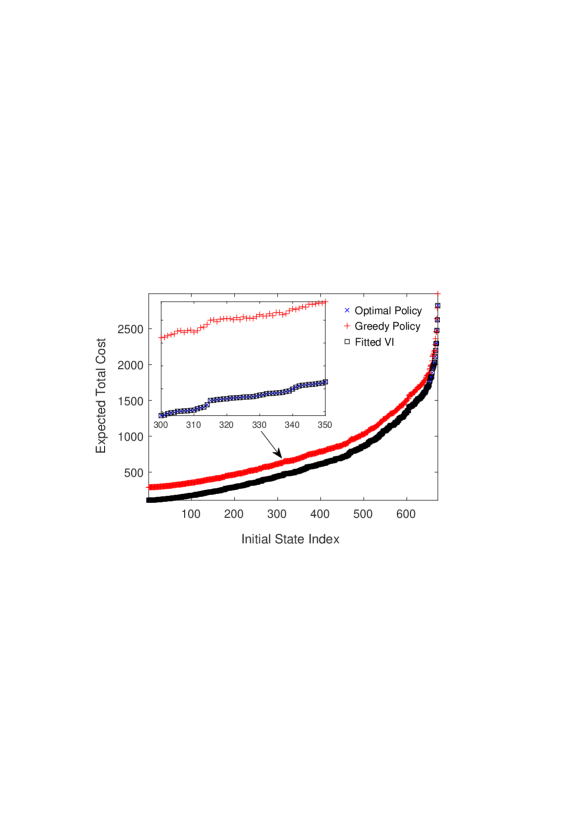
Figure 10: Expected total cost of optimal and greedy policies for each initial state with a suboptimal greedy policy when only 78% of the training set is used (see Text for details). Initial states are indexed from 1 to 672. Fitted VI remains optimal (Inset). The benchmark horizon is 400 time periods, and $p=0.4$.

In Fig 10, the benchmark is used with a $\times 4$ sparse code leading to 1323 states (a small number of states is used here as it is easier to visualize graphically). Of these, 1031 states have at least one non-negative coordinate (i.e., 78% of the total number of states). These states are used as the training set. Fitted value iteration is then applied to find optimal policies for the 672 initial states with suboptimal greedy policies. Fig 10 shows these policies remain optimal policies under the proposed sampling strategy. However, decreasing the training set below 78% of the total number of states rapidly degrades performance as states from the relevant partition start to be left out of the training set. The benchmark provides an ideal testing ground to investigate these types of behaviours.

4 Discussion and Conclusions

This work provides three main new contributions to the reinforcement learning methodology for solving Markov decision processes and optimal control tasks.

Defining an optimal control problem for a sequence of natural images requires understanding how the problem can be formulated, and what types of solution we can expect. We derived the general conditions for an image to be sufficient for implementing an optimal policy by drawing on an analogy with belief states in partially observed Markov decision processes. The first, and most obvious, condition is that an image must contain all task-dependent information required for the optimal control task at hand so that the cost or reward of each time period can be determined. The second, less obvious, condition is that we must have access to a mechanism for generating new images, where the next image is determined by the current image and the control we choose at the current time period. An image generator such as this is necessary for capturing the dynamics of moving through an environment under a sequential decision process when each state of the environment is an image.

This work also contributed a novel reinforcement learning benchmark for comparing different image representations. The benchmark scales easily so that large numbers of states can be considered for both finite and infinite horizons. This was necessary to convincingly demonstrate the scalability of efficient image representations to large tasks with many states. The benchmark implements a particularly simple image generator, making use of natural image patches and generative stochastic dynamics motivated by target tracking in natural video. This approach allows a simple cost per time period to be implemented, and optimal policies to be easily distinguished from suboptimal policies. More generally, a useful practical image generator might comprise a camera attached to an autonomous vehicle with kinematic controls, or a future generative AI technology that can generate natural images or video frames given some partial information about the environment.

The main contribution of this work was to propose and demonstrate the effectiveness of overcomplete sparse codes as natural image representations that are computationally efficient for optimal control. This work is a significant extension of previous results in this area achieved without a scalable benchmark (Loxley, 2021). When a linear network is used to find optimal policies for image sequences, computationally efficient image representations were shown to lead to faster network training with fewer least-squares iterations, and to minimal-sized networks for storing the input-output associations in training sets. Therefore, these representations use fewer computational resources to learn and evaluate optimal policies. As a result, it now becomes possible to consider larger tasks with more states. The best result presented here was finding an optimal policy for a task with 21675 natural images at each time period, with each image of size 361 pixels. This result was achieved using a $\times 64$ sparse code (at 94% efficiency), with the size of the task approximately three orders of magnitude larger (in base 4) than could be achieved using any complete code; for example, one generated using independent component analysis.

Computationally efficient representations were shown to be both overcomplete and sparse. By considering an overcomplete natural image, it was demonstrated that overcompleteness alone is not sufficient for increasing the storage capacity of a linear network. Similarly, sparseness alone is not sufficient. Only by combining both properties to get an overcomplete sparse code is this computational efficiency exhibited. The underlying reason is due to the form of the design matrix for the least-squares problem of network training. Provided the number of states is not larger than the size of the overcomplete sparse code, the design matrix is approximately square. Sparsity then approximately decorrelates neighbouring pixels in the input image, maximizing the rank of the design matrix. In turn, this maximizes the storage capacity of the network and leads to a more favourable condition number for the Hessian matrix.

An interesting question now becomes: what is the limit to overcompleteness for sparse image representations? In this work, we looked at $\times 4$, $\times 16$, and $\times 64$ overcomplete sparse codes. Might it be possible to continue to increase the degree of overcompleteness, and thereby continue to increase the storage capacity of a linear network for an input of fixed size? Achieving this may require a more sophisticated approach to sparsity. Here, we employed a very simple method for generating overcomplete sparse codes. It is possible to achieve sparser codes with alternative algorithms, such as those described in Olshausen (2013), and Rehn and Sommer (2007).

In this work, we also used the benchmark to explore affects due to the length of the horizon, alternative sampling strategies, and the partition of states into greedy optimal and suboptimal policies. We showed it was not necessary to train on all states in order to find suboptimal greedy policies. We also showed that for some initial states, suboptimal greedy policies only develop as the length of the horizon increases. An infinite horizon analysis confirmed the existence of stationary policies that are suboptimal. The benchmark provides an ideal testing ground to investigate these types of behaviours.

The work presented here is highly relevant to anyone interested in developing efficient solution methods for Markov decision processes or optimal control tasks involving natural image sequences or natural video frames. It may also be relevant more generally for optimal control with other types of high-dimensional data that lead naturally to sparse codes. Sparse codes can be generated by devices with low energy requirements (Fair et al., 2019), and have a much lower computational overhead when compared with competing AI methodologies such as deep learning. This makes overcomplete sparse codes worthy of consideration for optimal control applications.

Appendix A1: Method for generating overcomplete sparse codes

The method used here to generate overcomplete sparse codes of a natural images is taken from Loxley (2017, 2021), and starts with the (real-valued) two-dimensional (2D) Gabor function given by:

$$G({r},{r}^{\prime})=A\exp{\left[-\frac{1}{2}\left(\frac{\tilde{i}^{2}}{\sigma_{x}({r}^{\prime})^{2}}+\frac{\tilde{j}^{2}}{\sigma_{y}({r}^{\prime})^{2}}\right)\right]}\cos{\left[k({r}^{\prime})\tilde{j}+\varphi({r}^{\prime})\right]},$$ (20)

and

$$(\tilde{i},\tilde{j})=\left(\begin{array}[]{cc}\cos{\phi({r}^{\prime})}&-\sin{\phi({r}^{\prime})}\\ \sin{\phi({r}^{\prime})}&\cos{\phi({r}^{\prime})}\\ \end{array}\right)\left(\begin{array}[]{c}i-x_{0}({r}^{\prime})\\ j-y_{0}({r}^{\prime})\\ \end{array}\right),$$ (21)

where $k({r}^{\prime})=2\pi/\lambda({r}^{\prime})$; and where ${r}=(i,j)$ and ${r}^{\prime}=(i^{\prime},j^{\prime})$ are discrete two-dimensional coordinates. When the 2D Gabor function is adapted to natural image statistics, the three spatial Gabor parameters $\sigma_{x},\sigma_{y},$ and $\lambda$ are found to be strongly correlated and have heavy-tailed distributions (Loxley, 2017). The joint probability density of these parameter values is approximated using the sampling scheme in Table 4, and described by a Gaussian copula with Pareto marginal distributions.

Gabor Parameter(s)	Sample Transformation
$\sigma_{x}^{\prime},\sigma_{y}^{\prime},\lambda^{\prime}$	$(\sigma_{x}^{\prime},\sigma_{y}^{\prime},\lambda^{\prime})=(1,1,\rho)z$
$\sigma_{x}$	$\sigma_{x}={\cal{PCDF}}^{-1}({\cal{NCDF}}(\sigma_{x}^{\prime}|0,1)|\alpha_{1},\beta_{1})$
$\sigma_{y}$	$\sigma_{y}={\cal{PCDF}}^{-1}({\cal{NCDF}}(\sigma_{y}^{\prime}|0,1)|\alpha_{2},\beta_{2})$
$\lambda$	$\lambda={\cal{PCDF}}^{-1}({\cal{NCDF}}(\lambda^{\prime}|0,1)|\alpha_{3},\beta_{3})$

Table 4: Sampling scheme for the three spatial Gabor function parameters: sample $z\sim{\cal{N}}(0,1)$ from the standard normal distribution, then apply the parameter transformations listed in the table. Here, $\rho,\alpha_{i}$, and $\beta_{i}$ are model parameters, ${\cal{PCDF}}^{-1}(x|\alpha,\beta)=\frac{\beta}{(1-x)^{1/\alpha}}$ is the inverse CDF for the Pareto distribution, and ${\cal{NCDF}}(x|0,1)$ denotes the CDF for the standard normal distribution.

Due to the Pareto marginal distributions the sampling scheme is length scale invariant. Scale invariance is a key property of natural images. The resulting set of randomly generated Gabor functions are therefore self-similar and multiscale in the same way as self-similar multiresolution wavelet schemes. All other Gabor parameters are sampled uniformly over their respective ranges.

In the first step, a sample is collected for each of the seven Gabor parameters $(\phi,\varphi,\sigma_{x},\sigma_{y},\lambda,x_{0},y_{0})$, leading to a single 2D Gabor function indexed by a value of ${r}^{\prime}$. This step is repeated $m$ times; leading to $m$ Gabor functions indexed by $m$ unique values of ${r}^{\prime}$. Two-dimensional Gabor functions are not orthogonal. However, given an image $I({r})\in\mathbb{R}^{d}$, it is possible to find its sparse code $a({r}^{\prime})\in\mathbb{R}^{m}$ using a least-squares approximation. Letting $G\in\mathbb{R}^{d\times m}$ be a matrix with elements $G({r},{r}^{\prime})$, the sparse code $a({r}^{\prime})$ is found by solving the least-squares problem,

$$\text{minimize}\ \ \ \lVert Ga-I\rVert_{2}^{2}$$

$$\text{subject to}\ \ \ a\in\mathbb{R}^{m}.$$

When $m>d$, the sparse code is overcomplete; meaning that there are more Gabor function coefficients than image pixels.

Appendix A2: Infinite horizon policy evaluation

A stationary policy is a policy that does not change with each time period $k$, and can therefore be written as $\pi=\{\mu(i),\mu(i),...\}$. In Sec. 3.1, we identified two stationary policies. We would now like to find the their expected total costs in the infinite horizon limit (i.e., as $N\rightarrow\infty$). To work in this limit, we must introduce a discount factor $0<\alpha\leq 1$ that prevents total costs from becoming infinite. For any stationary policy $\mu$, the expected total costs $J_{\mu}(1),...,J_{\mu}(n)$ are then found as the unique solution to the following system of linear equations:

$$J_{\mu}(i)=g(i)+\alpha\sum_{j}p_{ij}(\mu(i))J_{\mu}(j).$$ (22)

The stationary optimal policy identified in Sec. 3.1 is given by $\mu^{*}((0,1),(0,0))=(1,0)$, $\mu^{*}((0,0),(1,1))=(0,1)$, and $\mu^{*}((0,0),(0,1))=(0,1)$. These states have a cost per time period given by $g((0,1),(0,0))=1$, $g((0,0),(1,1))=0$, and $g((0,0),(0,1))=0$. After rearranging Eq. (22) as

$$\sum_{j}\big{(}\delta_{ij}-\alpha p_{ij}(\mu(i))\big{)}J_{\mu}(j)=g(i),$$ (23)

the linear system can be written as $\boldsymbol{AJ}_{\mu}=\boldsymbol{g}$, where

$$\boldsymbol{A}=\begin{bmatrix}1&-\alpha&0\\ 0&1&-\alpha\\ -\alpha(1-p)&0&1-\alpha p\end{bmatrix},$$ (24)

so that $\det{(\boldsymbol{A})}=1-\alpha p-\alpha^{3}(1-p)$. For the stationary optimal policy, $\boldsymbol{g}$ is given by $[1,0,0]^{\top}$, and it is easily confirmed that $\boldsymbol{AJ}_{\mu}^{*}=[1,0,0]^{\top}$ is solved by

$$\boldsymbol{J}_{\mu}^{*}=\begin{bmatrix}1-\alpha p\\ \alpha^{2}(1-p)\\ \alpha(1-p)\end{bmatrix}\times(1-\alpha p-\alpha^{3}(1-p))^{-1}.$$ (25)

The stationary greedy policy identified in Sec. 3.1 is given by $\mu^{G}((0,0),(0,0))=(1,0)$, $\mu^{G}((0,-1),(1,1))=(0,1)$, and $\mu^{G}((0,-1),(0,1))=(0,1)$. These states have a cost per time period given by $g((0,0),(0,0))=0$, $g((0,-1),(1,1))=1$, and $g((0,-1),(0,1))=1$. Now $\boldsymbol{g}$ is given by $[0,1,1]^{\top}$. It can then be confirmed that $\boldsymbol{AJ}_{\mu}^{G}=[0,1,1]^{\top}$ is solved by

$$\boldsymbol{J}_{\mu}^{G}=\begin{bmatrix}\alpha+\alpha^{2}(1-p)\\ 1+\alpha(1-p)\\ 1+\alpha^{2}(1-p)\end{bmatrix}\times(1-\alpha p-\alpha^{3}(1-p))^{-1}.$$ (26)

The expected total cost ratio $\boldsymbol{J}_{\mu}^{G}/\boldsymbol{J}_{\mu}^{*}$, for the first greedy state $i^{G}_{1}=(0,0),(0,0)$, and the first optimal state $i^{*}_{1}=(0,1),(0,0)$, is

$$\frac{J_{\mu}^{G}(i^{G}_{1})}{J_{\mu}^{*}(i^{*}_{1})}=\alpha+\frac{\alpha^{2}}{1-\alpha p}.$$ (27)

Taking the limit of zero discounting (i.e., $\alpha\rightarrow 1$), Eq. (27) becomes

$$\lim_{\alpha\rightarrow 1}\frac{J_{\mu}^{G}(i^{G}_{1})}{J_{\mu}^{*}(i^{*}_{1})}=1+\frac{1}{1-p}.$$ (28)

This ratio describes the gap in the expected total cost between the greedy and optimal policies in the infinite horizon limit, and is useful for comparing with the finite horizon results of Sec 3.1. Some useful values include: 2 (when $p=0$), 5 (when $p=0.75$), and $1/(1-p)$ as $p\rightarrow 1$. Alternatively, for $p=1$, the original expression (27) gives $1/(1-\alpha)$ as $\alpha\rightarrow 1$.

Appendix A3: Efficient evaluation of the expected total cost

An efficient method is now presented for evaluating the expected total cost,

$${\mathbb{E}}\left\{\sum_{k=0}^{N-1}g_{k}(i_{k},\mu_{k}(i_{k}),i_{k+1})\right\}.$$

The key to an efficient evaluation is to make use of the Markov property to decompose the joint probability distribution $p(i_{0},i_{1},...,i_{N})$ into a product of transition probabilities: $p_{i_{0}}p_{i_{0}i_{1}}p_{i_{1}i_{2}}...p_{i_{N-1}i_{N}}$; where each transition probability $p_{i_{k}i_{k+1}}(\mu_{k}(i_{k}))$ has been abbreviated as $p_{i_{k}i_{k+1}}$. It is then possible to write the expected total cost as:

$${\mathbb{E}}\left\{\sum_{k=0}^{N-1}g_{k}(i_{k},\mu_{k}(i_{k}),i_{k+1})\right\}$$

$$=\sum_{i_{0}}p_{i_{0}}\sum_{i_{1}}p_{i_{0}i_{1}}g_{0}(i_{0},\mu_{0}(i_{0}),i_{1})$$

$$\ \ \ \ +\sum_{i_{0}}p_{i_{0}}\sum_{i_{1}}p_{i_{0}i_{1}}\sum_{i_{2}}p_{i_{1}i_{2}}g_{1}(i_{1},\mu_{1}(i_{1}),i_{2})$$

$$\ \ \ \ +...+\sum_{i_{0}}p_{i_{0}}...\sum_{i_{N-1}}p_{i_{N-2}i_{N-1}}\sum_{i_{N}}p_{i_{N-1}i_{N}}g_{N-1}(i_{N-1},\mu_{N-1}(i_{N-1}),i_{N}).$$

The number of evaluations here is formidable: the last term is a product of $N$ sums, each over $|S|$ states; leading to $|S|^{N}$ evaluations. We can do much better than this by taking advantage of the Markov property of the transition probabilities. Defining the following recurrence relation:

$$f_{i_{0}} =p_{i_{0}},$$ (29)

$$f_{i_{k}} =\sum_{i_{k-1}}f_{i_{k-1}}p_{i_{k-1}i_{k}},$$ (30)

allows the previous equation to be written as:

$${\mathbb{E}}\left\{\sum_{k=0}^{N-1}g_{k}(i_{k},\mu_{k}(i_{k}),i_{k+1})\right\}$$

$$=\sum_{i_{0}}f_{i_{0}}\sum_{i_{1}}p_{i_{0}i_{1}}g_{0}(i_{0},\mu_{0}(i_{0}),i_{1})$$

$$\ \ \ \ +\sum_{i_{1}}f_{i_{1}}\sum_{i_{2}}p_{i_{1}i_{2}}g_{1}(i_{1},\mu_{1}(i_{1}),i_{2})$$

$$\ \ \ \ +...+\sum_{i_{N-1}}f_{i_{N-1}}\sum_{i_{N}}p_{i_{N-1}i_{N}}g_{N-1}(i_{N-1},\mu_{N-1}(i_{N-1}),i_{N}),$$

$$=\sum_{k=0}^{N-1}\sum_{i_{k}}f_{i_{k}}\sum_{i_{k+1}}p_{i_{k}i_{k+1}}g_{k}(i_{k},\mu_{k}(i_{k}),i_{k+1}).$$

Now we only need to perform $O(N|S|^{2})$ evaluations given by the product of two sums over $|S|$ states, followed by a sum over $N$ time periods. However, when the number of states $|S|$ is large, $O(N|S|^{2})$ evaluations is still inefficient. A further simplification of the total expected cost results for our particular form of the cost per time period $g_{k}$, leading to:

$${\mathbb{E}}\left\{\sum_{k=0}^{N-1}g_{k}(i_{k})\right\}=\sum_{k=0}^{N-1}\sum_{i_{k}}f_{i_{k}}g_{k}(i_{k}).$$ (31)

Upon defining $i_{k-1}=(a_{1},b_{1})$ and $i_{k}=(a_{2},b_{2})$, Eq. (30) can be written as

$$f_{(a_{2},b_{2})}=\sum_{a_{1},b_{1}}f_{(a_{1},b_{1})}p(b_{2}|b_{1})\delta(a_{2}-(a_{1}+\mu(a_{1},b_{1})-b_{2})),$$

where Eq. (15) was used for $p_{i_{k-1}i_{k}}$. Multiplying by $g_{k}(i_{k})$, and summing over $i_{k}=(a_{2},b_{2})$, then leads to

$$\sum_{i_{k}}f_{i_{k}}g_{k}(i_{k})=\sum_{a_{1},b_{1},b_{2}}f_{(a_{1},b_{1})}p(b_{2}|b_{1})g_{k}(a_{1}+\mu(a_{1},b_{1})-b_{2},b_{2}).$$

Since $a_{1}\in D$ and $b_{1},b_{2}\in T$, this sum is $O(|S|)$ because the number of states can be written as $|S|=|D||T|$; and $|T|=3$. Using this sum in Eq. (31), we see that the total number of evaluations required to determine the expected total cost is $O(N|S|)$.

References

- Bell and Sejnowski [1997] Anthony J. Bell and Terrence J. Sejnowski. The “independent components” of natural scenes are edge filters. Vision Research, 37(23):3327–3338, 1997.
- Bertsekas [2017] D. P. Bertsekas. Dynamic programming and optimal control vol 1, 4th ed. Athena Scientific, 2017.
- Bertsekas [2019] D. P. Bertsekas. Reinforcement learning and optimal control. Athena Scientific, 2019.
- Daugman [1988] J.G. Daugman. Complete discrete 2-d gabor transforms by neural networks for image analysis and compression. IEEE Transactions on Acoustics, Speech, and Signal Processing, 36(7):1169–1179, 1988.
- Daugman [1989] J.G. Daugman. Entropy reduction and decorrelation in visual coding by oriented neural receptive fields. IEEE Trans. Biomed. Eng., 36:107–114, 1989.
- Daugman [1985] John G. Daugman. Uncertainty relation for resolution in space, spatial frequency, and orientation optimized by two-dimensional visual cortical filters. J. Opt. Soc. Am. A, 2(7):1160–1169, 1985.
- Fair et al. [2019] Kaitlin L. Fair, Daniel R. Mendat, Andreas G. Andreou, Christopher J. Rozell, Justin Romberg, and David V. Anderson. Sparse coding using the locally competitive algorithm on the truenorth neurosynaptic system. Frontiers in Neuroscience, 13, 2019.
- Field [1987] David J. Field. Relations between the statistics of natural images and the response properties of cortical cells. J. Opt. Soc. Am. A, 4(12):2379–2394, Dec 1987.
- Field [1994] David J. Field. What is the goal of sensory coding? Neural Computation, 6(4):559–601, 1994.
- Geisler and Perry [2011] Wilson Geisler and Jeff Perry. Statistics for optimal point prediction in natural images. Journal of vision, 11:14, 10 2011. doi: 10.1167/11.12.14.
- Hosseini et al. [2010] Reshad Hosseini, Fabian Sinz, and Matthias Bethge. Lower bounds on the redundancy of natural images. Vision Research, 50(22):2213–2222, 2010.
- Hubel and Wiesel [1959] D. H. Hubel and T. N. Wiesel. Receptive fields of single neurones in the cat’s striate cortex. The Journal of Physiology, 148(3):574–591, 1959.
- Hyvärinen et al. [2009] A. Hyvärinen, J. Hurri, and P. O. Hoyer. Natural Image Statistics. Springer-Verlag, 2009.
- Jones and Palmer [1987] J. P. Jones and L. A. Palmer. An evaluation of the two-dimensional gabor filter model of simple receptive fields in cat striate cortex. Journal of Neurophysiology, 58(6):1233–1258, 1987.
- Lange and Riedmiller [2010] Sascha Lange and Martin Riedmiller. Deep auto-encoder neural networks in reinforcement learning. pages 1–8, 09 2010.
- Le et al. [2017] Lei Le, Raksha Kumaraswamy, and Martha White. Learning sparse representations in reinforcement learning with sparse coding. In Proceedings of the Twenty-Sixth International Joint Conference on Artificial Intelligence, IJCAI-17, pages 2067–2073, 2017. doi: 10.24963/ijcai.2017/287.
- Li et al. [2024] Jianfei Li, Han Feng, and Ding-Xuan Zhou. Convergence analysis for deep sparse coding via convolutional neural networks, 2024. URL https://arxiv.org/abs/2408.05540.
- Liu et al. [2018] Vincent Liu, Raksha Kumaraswamy, Lei Le, and Martha White. The utility of sparse representations for control in reinforcement learning, 2018. URL https://arxiv.org/abs/1811.06626.
- Loxley [2017] P. N. Loxley. The Two-Dimensional Gabor Function Adapted to Natural Image Statistics: A Model of Simple-Cell Receptive Fields and Sparse Structure in Images. Neural Computation, 29(10):2769–2799, 2017.
- Loxley [2021] P. N. Loxley. A sparse code increases the speed and efficiency of neuro-dynamic programming for optimal control tasks with correlated inputs. Neurocomputing, 426:1–13, 2021.
- Olshausen and Field [1996] Bruno Olshausen and David Field. Emergence of simple-cell receptive field properties by learning a sparse code for natural images. Nature, 381:607–9, 07 1996.
- Olshausen [2013] Bruno A. Olshausen. Highly overcomplete sparse coding. In Bernice E. Rogowitz, Thrasyvoulos N. Pappas, and Huib de Ridder, editors, Human Vision and Electronic Imaging XVIII, volume 8651 of Society of Photo-Optical Instrumentation Engineers (SPIE) Conference Series, page 86510S, March 2013.
- Olshausen and Field [1997] Bruno A. Olshausen and David J. Field. Sparse coding with an overcomplete basis set: A strategy employed by v1? Vision Research, 37(23):3311–3325, 1997.
- Papyan et al. [2017] Vardan Papyan, Yaniv Romano, and Michael Elad. Convolutional neural networks analyzed via convolutional sparse coding. J. Mach. Learn. Res., 18(1):2887–2938, January 2017. ISSN 1532-4435.
- Rafati and Noelle [2019] Jacob Rafati and David C. Noelle. Learning sparse representations in reinforcement learning, 2019. URL https://arxiv.org/abs/1909.01575.
- Rehn and Sommer [2007] Martin Rehn and Friedrich T Sommer. A network that uses few active neurones to code visual input predicts the diverse shapes of cortical receptive fields. Journal of Computational Neuroscience, 22(2):135–146, 2007.
- Ruderman [1997] Daniel L. Ruderman. Origins of scaling in natural images. Vision Research, 37(23):3385–3398, 1997.
- Ruderman and Bialek [1994] Daniel L. Ruderman and William Bialek. Statistics of natural images: Scaling in the woods. Phys. Rev. Lett., 73:814–817, 1994.
- Simoncelli and Olshausen [2001] E. P. Simoncelli and B. Olshausen. Natural image statistics and neural representation. Annual Review of Neuroscience, 24:1193–1216, 2001.
- Sipser [2012] Michael Sipser. Introduction to the Theory of Computation. Course Technology, third edition, 2012.
- Zhang et al. [2018] Amy Zhang, Yuxin Wu, and Joelle Pineau. Natural environment benchmarks for reinforcement learning. arXiv, 2018. doi: 10.48550/arXiv.1811.06032.
- Zhang et al. [2021] Amy Zhang, Rowan McAllister, Roberto Calandra, Yarin Gal, and Sergey Levine. Learning invariant representations for reinforcement learning without reconstruction. arXiv, 2021. doi: 10.48550/arXiv.2006.10742.