LV-CadeNet: Long View Feature Convolution-Attention Fusion Encoder-Decoder Network for Clinical MEG Spike Detection

Abstract

It is widely acknowledged that the epileptic foci can be pinpointed by source localizing interictal epileptic discharges (IEDs) via Magnetoencephalography (MEG). However, manual detection of IEDs, which appear as spikes in MEG data, is extremely labor intensive and requires considerable professional expertise, limiting the broader adoption of MEG technology. Numerous studies have focused on automatic detection of MEG spikes to overcome this challenge, but these efforts often validate their models on synthetic datasets with balanced positive and negative samples. In contrast, clinical MEG data is highly imbalanced, raising doubts on the real-world efficacy of these models. To address this issue, we introduce LV-CadeNet, a Long View feature Convolution-Attention fusion Encoder-Decoder Network, designed for automatic MEG spike detection in real-world clinical scenarios. Beyond addressing the disparity between training data distribution and clinical test data through semi-supervised learning, our approach also mimics human specialists by constructing long view morphological input data. Moreover, we propose an advanced convolution-attention module to extract temporal and spatial features from the input data. LV-CadeNet significantly improves the accuracy of MEG spike detection, boosting it from 42.31% to 54.88% on a novel clinical dataset sourced from Sanbo Brain Hospital Capital Medical University. This dataset, characterized by a highly imbalanced distribution of positive and negative samples, accurately represents real-world clinical scenarios.

1 Introduction

Magnetoencephalography (MEG) facilitates the precise and non-invasive localization of epileptic foci by meticulously identifying and mapping the origins of epileptic spikes [1, 2]. This technique plays a pivotal role in the thorough preoperative diagnostic evaluation for patients being considered for surgical removal of epileptogenic lesions. In the current clinical workflow for localizing epileptic foci using MEG, manually annotating spikes from vast amounts of MEG data is the most time-consuming step. Thus, while the high temporal-spatial resolution of MEG offers the advantage of precise lesion localization for clinical purposes, it also imposes a significant burden on healthcare professionals who manually review MEG data. Consequently, automating the spike detection process holds considerable clinical value.

Many studies have investigated the automation of epileptic spike detection in MEG and Electroencephalogram (EEG) data over the past two decades [3]. Early works in this field focus on feature engineering, extracting information from the raw data in both the time and frequency domains, or a combination thereof, to construct the input for traditional machine learning models such as linear models and Support vector machines. These models are then employed to classify the input as either containing an epileptic spike or not [4, 5, 6]. While these approaches offer high interpretability of their decision-making processes, they often struggle with generalization due to the need for rigid parameter settings tailored to specific datasets. Recently, deep learning techniques have propelled MEG and EEG spike detection to new levels of performance. For example, the networks EMS-Net and FAMED proposed in [7, 8] have refined their convolutional neural network architectures to enhance feature extraction from the input MEG slice data, resulting in high detection precision on a large-scale MEG test dataset. In the realm of EEG spike detection, a variety of deep learning research has flourished. In addition to the convolutional architectures like SpikeNet [9], studies have also employed recurrent neural network [10] and graph neural network [11] to enhance detection capabilities. Furthermore, hybrid models that integrate convolutional and attention mechanisms [12] as well as multimodal approaches that concatenate diverse input sources [13, 14] have been developed for spike detection. These approaches have yielded promising results in the field of EEG spike detection.

However, a pivotal issue arises from the fact that nearly all previous studies have primarily validated their MEG spike detection models on data sets with a balanced distribution of positive and negative samples. In stark contrast, clinical data encountered in practical settings are severely imbalanced. For example, within a one-minute (60,000ms) MEG data file in our dataset, there are, on average, as few as five spike segments according to the clinical data we have collected. If each spike segment lasts for 200ms, this translates to 295 non-spike segments, creating an overwhelmingly lopsided positive to negative sample ratio of 5:295. This raises doubts about the real-world applicability of current state-of-the-art (SOTA) models. To address this challenge, we assessed a range of SOTA MEG spike detection models on a real-world dataset collected from Sanbo Brain Hospital, Capital Medical University. This dataset includes data from 26 patients, with each MEG file containing a 10-minute continuous recording of a single patient’s examination. Using this dataset, the effectiveness of the SOTA models could be truly assessed. Regrettably, we found that almost all existing networks are challenged in achieving satisfactory results. These findings suggest that there remains a substantial gap before these models can reliably supplant the manual annotation of MEG spikes.

In order to truely serve the clinical practice, we propose a novel deep learning framework to improve the performance of MEG spike detection in real-world data from multiple perspectives.

Firstly, we have designed six input features that measure the morphological significance of the input signal segment over an extended time duration, augmenting the input signal segment needing to be classified as a spike event or not. We will term this strategy as constructing long view morphological input data throughout the subsequent content of this study. This approach mirrors the meticulous manual annotation process of human experts, who typically identify MEG spikes ranging from 27ms to 120ms [15] within a 5-10 second MEG signal context. In Contrast, current SOTA MEG spike detection models predominantly utilize short-time-span signal clips as their exclusive input. To the best of the authors’ knowledge, the longest clip length employed is one second, as introduced in SpikeNet [9] and FAMED [8]. This limitation makes it challenging for the model to differentiate spikes from background waves within such a short time window. By integrating the enhanced significance features from the broader perspective with the raw input segment, we effectively capture the key characteristics of spikes across a wider temporal spectrum, while avoiding the introduction of extraneous noise within the extended view.

Secondly, we introduce an advanced convolution and attention fusion module designed to extract features. This module leverages convolutional operations to extract temporal features and the attention mechanism to adeptly capture spatial information from the input. In clinical settings, spatial dipole (equivalent current dipole, ECD) features are just as vital as temporal features for the identification of MEG spikes [16, 17]. While previous research has primarily focused on temporal feature extraction for spike detection, with only a handful of studies considering spatial dipole features, our approach addresses this gap. EEG spike detection works such as EEG-ConvTransformer [13] and V2IED [14] have explored spatial topological features but necessitated multimodal inputs and were not directly applicable to MEG data. Additionally, Satelight [12] employed serial convolution and attention mechanisms but did not specifically focus on spatial information extraction. Our solution, however, integrates a multi-dimensional feature extraction block that concurrently captures both temporal waveform and spatial dipole features, enhancing the performance of MEG spike identification.

Thirdly, to alleviate the the disparity between training data distribution and clinical test data, we have implemented a semi-supervised learning strategy to adjust the distribution of training data and leverage knowledge distillation to steer the model fine-tuning process. As far as the authors know, this is the first study utilizing semi-supervised learning to regulate the training data distribution for MEG spike detection.

Table 1: Statistics of The Training and Test sets

Dataset	Subjects	MEG files	Spikes	Non-Spikes	Duration (hours)	Others
Sanbo-CMR	119	468	14780	17511	65.5	1146709 unannoted
Sanbo-Clinic	26	28	957	63931	3.68	755“ignored points”+2min “ignored intervals”

Figure 1: Distribution of spike counts for each patient within the test dataset Sanbo-Clinic.

2 Materials and method

2.1 Data acquisition and pre-processing

2.1.1 Datasets

The training data employed for this investigation, Sanbo-CMR, was collected from the Sanbo Brain Hospital Capital Medical University and the Center for MRI Research Peking University. It includes MEG files that are annotated with both spikes and non-spikes in a nearly balanced ratio, similar to previous MEG spike detection studies, alongside a significant portion of unannotated data. For the test data, we utilized a novel dataset Sanbo-Clinic collected from Sanbo Brain Hospital, where each MEG file was thoroughly annotated by neurophysiologists, resulting in a pronounced imbalance between positive and negative samples. In the test set, signal segments that the attending physician could not conclusively identify as spikes were annotated as “ignored” for individual data points or “ignored intervals” for signals of extended duration. Data with an “ignored" label does not count into the training and evaluation process. Comprehensive statistics of the training and test datasets are detailed in Table 1. We also present the distribution of spike counts for each patient in our Sanbo-Clinic test set in Fig. 1, reflecting the considerable variability observed in spike numbers across individuals. This research was approved by the Institutional Review Boards of the two participating centers, and all patients provided written consent.

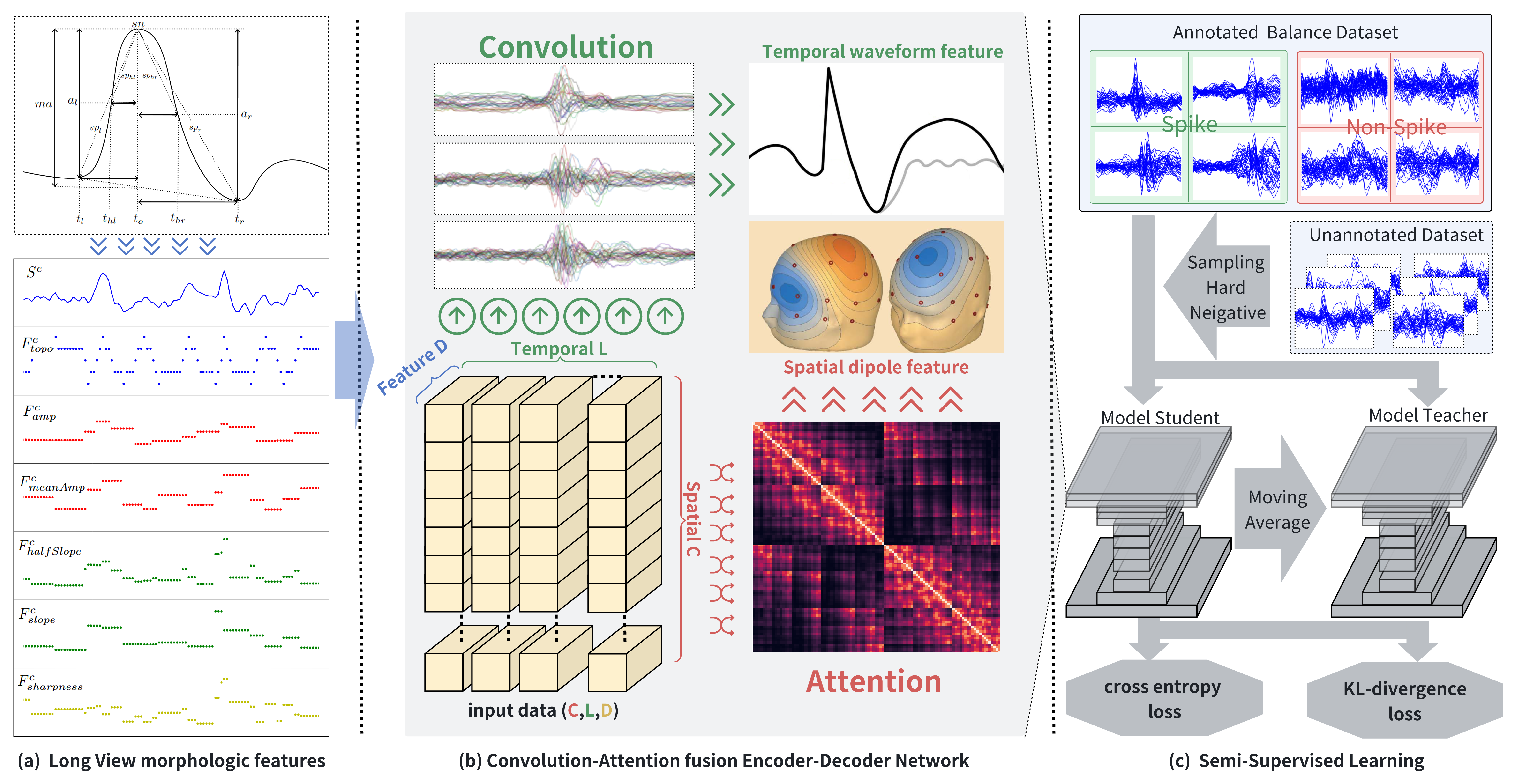
Figure 2: Overview of the Long View Feature Convolution-Attention fusion Encoder-Decoder Network. This framework ingests the long view input data that we proposed and constructed. It then processes this data using CadeNet, which integrates attention mechanisms and convolutional blocks to extract features for prediction. CadeNet is initially trained on annotated data and subsequently fine-tuned with a semi-supervised learning scheme. (a) Diagram of the long view input data we constructed. (b) Workflow of CadeNet, leveraging the attention mechanism to capture spatial dipole features among various channels of the input data, and convolutional blocks to facilitate the temporal propagation features inherent to the input. Subfigures depicting the MEG spike and dipole features located on the top right corner are borrowed from [17]. (c) Overview of the semi-supervised learning scheme and knowledge distillation process.

2.1.2 Prepocessing approaches

The preprocessing pipeline comprises six integral steps: (1) application of the Maxwell Filter [18] to mitigate external interferences; (2) artifact reduction associated with electrooculogram (EOG) and electrocardiogram (ECG) data via Independent Component Analysis; (3) isolation of relevant frequency bands through implementation of a 3-40 Hz band-pass filter; (4) reduction of computational complexity by downsampling all data to a rate of 250Hz; (5) computation of mean amplitude values and standard deviations for the signals within each MEG file, followed by normalization of data using the z-score method. (6) utilization of data augmentation strategies, including the addition of Gaussian noise and the random nullification of channels of the input. Step 6 is discarded for the MEG files within the test dataset.

2.2 LV-CadeNet: Long View feature Convolution-Attention fusion Encoder-Decoder Network

For a preprocessed MEG signal file $\mathcal{S}\in\mathbb{R}^{C\times T}$, representing the $C$-channel signal variations across a time duration of $T$, the objective of our LV-CadeNet approach is to identify whether each signal segment $S$ within $\mathcal{S}$ exhibit epileptic spikes. To achieve this, we first construct the long view input features $\mathcal{F}$ for $\mathcal{S}$. Subsequently, we propose an advanced convolution-attention fusion model, CadeNet, to extract features from $\mathcal{X}=[\mathcal{S},\mathcal{F}]$, and harbors spikes using a segmentation head. Semi-supervised learning is utilized to optimize the distribution of training data and the learning mechanics of CadeNet. Ultimately, a series of postprocessing steps are applied to locate the spiking time point within $\mathcal{X}$. An illustration of LV-CadeNet is presented in Fig. 2, with a detailed explanation of its components provided in the subsequent four sections.

$$a_{l} =\mathcal{S}^{c,t_{o}}-\mathcal{S}^{c,t_{l}};a_{r}=\mathcal{S}^{c,t_{r}}-\mathcal{S}^{c,t_{o}}$$ (1)

$${sp}_{l} =\frac{a_{l}}{t_{o}-t_{l}};{sp}_{r}=\frac{a_{r}}{t_{r}-t_{o}}$$ (2)

$$hsp_{l} =\frac{a_{l}}{2\cdot(t_{o}-t_{hl})};hsp_{r}=\frac{a_{r}}{2\cdot(t_{hr}-t_{o})}$$ (3)

$$ma =\frac{a_{l}\cdot(t_{r}-t_{o})+a_{r}\cdot(t_{o}-t_{l1}}{t_{r}-t_{l}})$$ (4)

$$sn =\left|\textstyle\sum^{t_{o}+4}_{t=t_{o}-4}\mathcal{S}^{c,t}-9\cdot\mathcal{S}^{c,t_{o}}\right|$$ (5)

2.2.1 Long view input feature construction

To generate the long view input feature $F$ for a given input signal segment $S$, we initiate the process by leveraging the file-level signal $\mathcal{S}$ to derive the file-level feature $\mathcal{F}$ with the three-step process outlined below.

Firstly, we identify the local maxima and minima in $\mathcal{S}$ through extremum detection, considering a wave with a maximum moment $t_{o}$ between two minima $t_{l},t_{r}$ as a complete wave [19]. Using this method, the signal of each channel $\mathcal{S}^{c}$ where $c$ ranges from 0 to $C$ can be divided into a certain number of complete waves.

Secondly, we construct six features for each signal $\mathcal{S}^{c}$. The first feature depicting topological structure of $\mathcal{S}^{c}$ is denoted as $\mathcal{F}^{c}_{topo}$. More specifically, signals at local maxima are assigned a value of 1 for $\mathcal{S}^{c}$. Conversely, signals at local minima are assigned a value of -1. For signals occurring at the half-width high points, which lie between local maxima and minima, a value of 0 is attributed. Signals at other time points are assigned values of 0.5 or -0.5, depending on their proximity to the local maxima or minima, respectively. The other five features are represented as $\mathcal{F}^{c}_{amp}$, $\mathcal{F}^{c}_{meanAmp}$, $\mathcal{F}^{c}_{slope}$, $\mathcal{F}^{c}_{halfSlope}$ and $\mathcal{F}^{c}_{sharpness}$, each providing insights into a distinct morphological property of $\mathcal{S}^{c}$. To construct these features, we first calculate key properties for a single complete wave. Taking the wave with a time ranging from $t_{l}$ to $t_{o}$ to $t_{r}$ within $\mathcal{S}^{c}$ as an example, we define the left and right adjacent half-width high moments as $t_{hl}$ and $t_{hr}$ respectively. Then the basic properties of this wave can be computed with Equations (1)-(5). In these formulas, $a$, $sp$, $hsp$, and $sn$ represent the abbreviations for the amplitude, slope, half-width slope and sharpness of the wave respectively [15], while $ma$ refers to the mean amplitude of the wave. “$l$" is used to denote properties of the left half of the wave, and “$r$" is used to denote properties of the right half of the wave. Utilizing these essential wave characteristics, we can construct the six features that align with the shape of $\mathcal{S}^{c}\in\mathbb{R}^{1\times T}$ by interpolating the available features across the time intervals. Specifically, for each single wave, the elements spanning from $t_{hl}$ to $t_{o}$ within matrix $\mathcal{F}^{c}_{amp}$ are denoted as $\mathcal{F}^{c,t_{hl}:t_{o}}_{amp}$ and assigned the value $a_{l}$. In alike manner, $\mathcal{F}^{c,t_{o}:t_{hr}}_{amp}$ receives the value $a_{r}$. For the feature related to mean amplitude, $\mathcal{F}^{c,t_{hl}:t_{hr}}_{meanAmp}$ is given the value $ma$. Regarding the slope-related feature, $\mathcal{F}^{c,t_{hl}:t_{o}}_{slope}$ acquires the value $sp_{l}$, and $\mathcal{F}^{c,t_{o}:t_{hr}}_{slope}$ acquires the value $sp_{r}$. For the feature related to half slope, $hsp_{l}$ is attributed to $\mathcal{F}^{c,t_{hl}:t_{o}}_{halfSlope}$ and $hsp_{r}$ is attributed to $\mathcal{F}^{c,t_{o}:t_{hr}}_{halfSlope}$. $\mathcal{F}^{c,t_{hl}:t_{hr}}_{sharpness}$ is assigned the value $sn$. Finally, we normalize the above five features across a 6-second interval. This interval is selected corresponding to the signal perspective essential for the manual annotation of spikes by our participating clinical experts. Since the feature construction approaches are applied to each $\mathcal{S}^{c}$, the resulting features are file-level features denoted as $\mathcal{F}_{topo}$, $\mathcal{F}_{amp}$, $\mathcal{F}_{meanAmp}$, $\mathcal{F}_{slope}$, $\mathcal{F}_{halfSlope}$, $\mathcal{F}_{sharpness}$ respectively, each having a dimension of (C, T).

Thirdly, we concatenate the six long view features introduced above with the signal $\mathcal{S}$ to form a long view feature matrix $\mathcal{X}\in\mathbb{R}^{C\times T\times 7}$ at the file-level. The input slice $X^{i}\in\mathbb{R}^{C\times L\times 7}$ is extracted by selecting the signal centered on the annotation point $i$ with a duration of $L$ from the file matrix $\mathcal{X}$. An intuitive diagram depicting the input $X^{i}$ is presented in Fig. 2. Subsequently, we aggregate a collection of slices into a batch represented as $X=[X^{b}|b\in[1,B]]\in\mathbb{R}^{B\times C\times L\times D}$ for training where $B$ represents the batch size. In the subsequent sections of this research, we refer to the first dimension of a feature matrix as the batch dimension, the second as the spatial or sensor dimension, the third as the temporal dimension, and the fourth as the feature dimension. This nomenclature is adopted to clarify and enhance the explanation of our methodology.

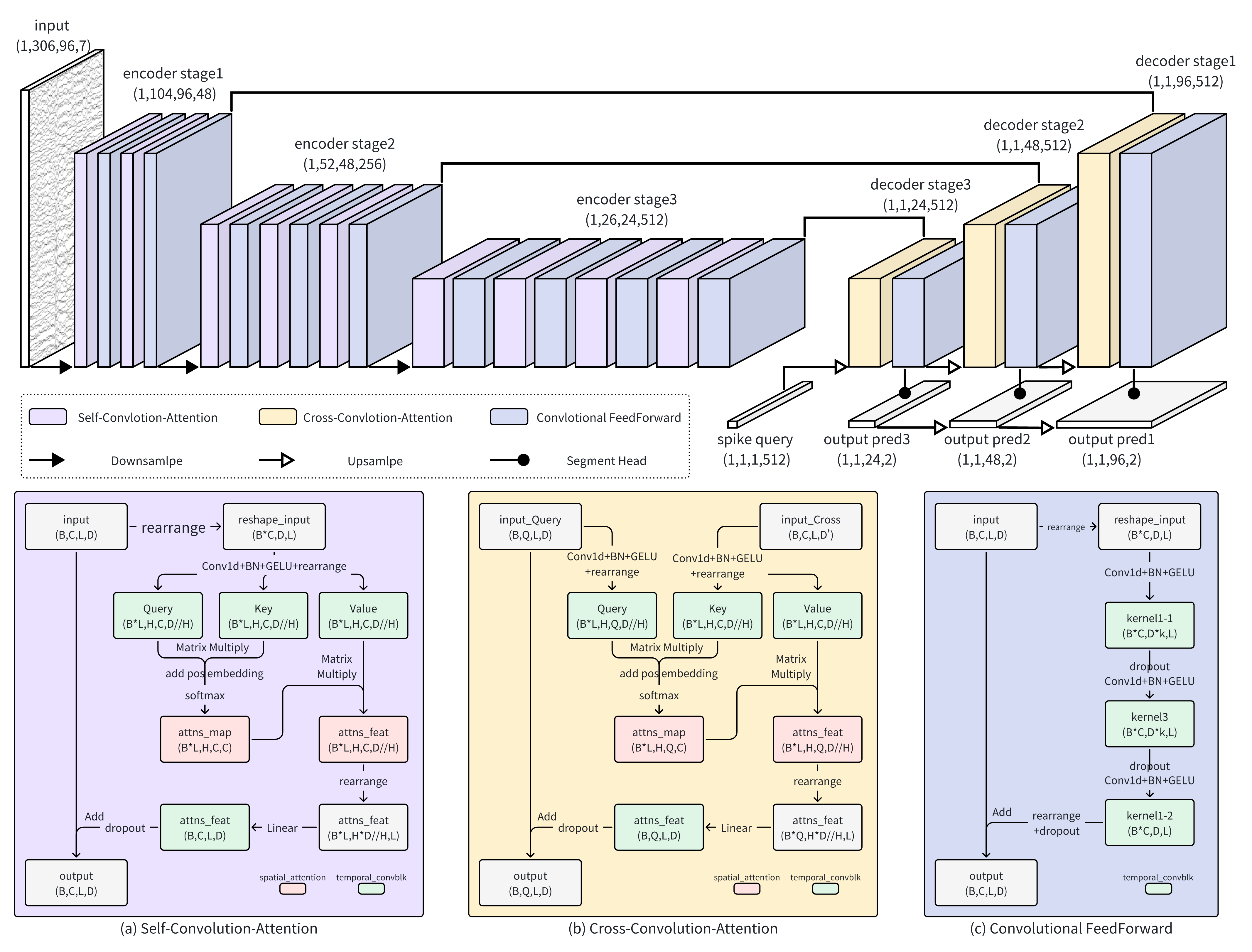
Figure 3: Architecture of our feature extraction model CadeNet when the batch size is 1 and structure of key modules within CadeNet. (a) Workflow of the self-convolution-attention block. (b) Workflow of the cross-convolution-attention block. (c) Workflow of the convolutional feedforward block.

2.2.2 Convolution-Attention fusion Encoder-Decoder Network

The CadeNet model we propose constitutes an encoder-decoder framework, where the encoder’s role is to distill essential features from the input $X$, while the decoder’s function is to synthesize these features along with an additional learnable vector for the purpose of prediction. The encoding and decoding operations are conducted across three stages, and the predictions yielded by various stages of the decoder are cumulatively combined to produce the final prediction. A detailed depiction of the CadeNet architecture is presented in Fig. 3. The subsequent discussion will explore the integral components that make up CadeNet. Within these components, a residual connection is integrated into each submodule within the convolution-attention and convolutional feedforward blocks. As a result, the output maintains the same dimensions as the input for these two blocks, ensuring a seamless flow of information.

Convolution-Attention Block. The convolution-attention block in CadeNet includes two parts: the self-convolution-attention module and the cross-convolution-attention module. For the self-convoloution-attention module, it’s input $Z_{slf}$ is a feature either transformed from the input $X$ or derived from the Downsample module of CadeNet. Suppose $Z_{slf}$ has a dimension of $(\hat{B},\hat{C},\hat{L},\hat{D})$, the following equations will be applied to $Z_{slf}$ to extract temporal and spatial features:

$$Z_{1} =ConvBlk(Z_{slf}\xrightarrow{Trans}\mathbb{R}^{(\hat{B}\cdot\hat{C})\times\hat{D}\times\hat{L}}),$$ (6)

$$Z_{1} \in\mathbb{R}^{(\hat{B}\cdot\hat{C})\times(3\cdot H_{slf}\cdot D_{slf})\times\hat{L}}$$

$$Z_{2} =Z_{1}\xrightarrow{Trans}\mathbb{R}^{3\times(\hat{B}\cdot\hat{L})\times H_{slf}\times\hat{C}\times D_{slf}}$$ (7)

$$Q_{slf} =Z_{2}[0,:];K_{slf}=Z_{2}[1,:];V_{slf}=Z_{2}[2,:]$$ (8)

$$Self Attention(Z_{1})=SoftMax(\frac{Q_{slf}\ast K_{slf}}{\sqrt{D_{slf}}})\ast V_{slf}$$ (9)

$$Z_{3} =MultiHead(SelfAttention(Z_{1})),$$ (10)

$$Z_{3} \in\mathbb{R}^{(\hat{B}\cdot\hat{L})\times H_{slf}\times\hat{C}\times D_{slf}}$$

$$Z_{4} =ConvBlk(Z_{3}\xrightarrow{Trans}\mathbb{R}^{(\hat{B}\cdot\hat{C})\times(H_{slf}\cdot D_{slf})\times\hat{L}})$$ (11)

$$Z^{\prime}_{slf} =Z_{slf}+(dropout(Z_{4})\xrightarrow{Trans}\mathbb{R}^{\hat{B}\times\hat{C}\times\hat{L}\times\hat{D}})$$ (12)

Where the $ConvBlk$ in the equations consists of a 1D convolutional layer operated along the temporal dimension, followed by a batch normalization layer[20] and GELU activation layer[21]. The $SelfAttention$ and $MultiHead$ are referenced from [22]. $H_{slf}$ and $D_{slf}$ represent the dimensionality for computing the query matrix $Q_{slf}$, the key matrix $K_{slf}$, and the value matrix $V_{slf}$. $dropout$ [23] is a function that prevents the convolution-attention block from overfitting. In subsequent experiments, the value of $H_{slf}$ is fixed at 8. $D_{slf}$ is determined through the division of $\hat{D}$ and $H_{slf}$, and a dropout ratio of 0.2 is applied.

For the cross-convolution-attention module, unlike the self-convolution-attention module which processes a single input, this module takes two inputs: the feature matrix $Z_{cros}$, which is the output from the encoder at a particular stage, and a learnable external feature matrix $Z_{query}$ either generated by CadeNet or an aggregated decoded feature derived from upsampling decoding features. The computation of the output for this module follows a similar approach to the self-convolution-attention module, with one key distinction: the Query vector $Q_{cros}$, which serves as an input to the multihead attention layer, is derived from the external feature matrix $Z_{query}$, analogous to how $Q_{slf}$ is derived from $Z_{slf}$. Concurrently, the Key and Value vectors $K_{cros}$ and $V_{cros}$, which are the other two inputs to the multihead attention layer, are obtained in the same manner as the self-convolution-attention module, from the encoder-produced feature matrix $Z_{cros}$.

Convolutional Feedforward Block. The convolutional feedforward module is utilized at every stage within both the encoder and decoder, subsequent to the convolution-attention module, as depicted in Fig. 3(c). This module intricately processes the feature derived from a particular convolution-attention block along the temporal axis. The feature, denoted as $Z_{ff}\in\mathbb{R}^{\hat{B}\times\hat{C}\times\hat{L}\times\hat{D}}$ retains the same dimensions as the input to the convolution-attention block due to the residual connections between submodules. To refine the temporal characteristics, we transform $Z_{ff}$ to a shape of $(\hat{B}\cdot\hat{C},\hat{D},\hat{L})$. Subsequently, three $ConvBlk$s with $dropout$ are applied to this transformed version of $Z_{ff}$. The process concludes with a residual connection linking the input and output, as illustrated by the following equations:

$$Z_{5} =Z_{ff}\xrightarrow{Trans}\mathbb{R}^{(\hat{B}\cdot\hat{C})\times\hat{D}\times\hat{L}}$$ (13)

$$Z_{conv} =(\prod^{3}dropout\odot ConvBlk)(Z_{5})$$ (14)

$$Z^{\prime}_{ff} =Z_{ff}+Z_{conv}\xrightarrow{Trans}\mathbb{R}^{\hat{B}\times\hat{C}\times\hat{L}\times\hat{D}}$$ (15)

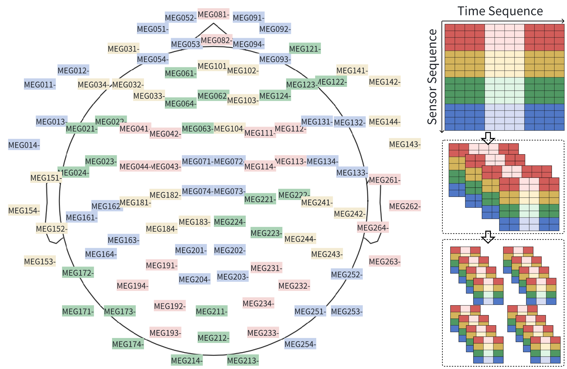
Figure 4: Illustration of the sensor groups, and the process to compress the input. The 306 sensors for the input are divided into 26 groups according to their numbering, each group having 12 sensors. The group originally having number of sensors less than 12 is padded with sensors from this group.

Downsample and Upsample Block. In this block, the downsampling layer is designed to condense the features $Z_{ds}\in\mathbb{R}^{\hat{B}\times\hat{C}\times\hat{L}\times\hat{D}}$. It specifically targets the spatial and temporal dimensions within the encoder, shifting this information to the feature dimension, which is essential for predictions in the decoder. The layer converts $Z_{ds}$ to $Z^{\prime}_{ds}\in\mathbb{R}^{\hat{B}\times\frac{\hat{C}}{p}\times\frac{\hat{L}}{q}\times(\hat{D}\cdot p\cdot q)}$. This information swap between different dimensionalities is achieved with two steps: first, the Pixel Shuffle method [24] is applied to compress the spatial or temporal data and integrate it into the feature dimension, followed by a one-dimension convolutional layer that adjusts the last feature dimension to desired size. It is worth noting that the parameter $p$ corresponds to the number of sensor groups generating the MEG signal, with sensors in close proximity within each group. This approach results in a more coherent and interpretable representation of the spatial information within the feature dimension. A diagram intuitively illustrating the sensor groups is presented in Fig. 4, where each color represents a distinct group.

The upsampling layer functions along the temporal axis to adjust the features within the decoder, ensuring the temporal dimension of these features match the time length that is to be predicted.

Segmentation head. Distinct from prior approaches that employ a classification head to predict a binary label for the entire input slice, our method employs a segmentation head that conducts binary classifications for every sampling point within the input slice. This segmentation head demonstrates enhanced robustness compared to the classification head, effectively mitigating the impact of noise contained within the slice. The segmentation head consists of a 1D convolutional operator that transforms the final output feature $Z_{pred}\in\mathbb{R}^{\hat{B}\times 1\times\hat{L}\times\hat{D}^{\prime}}$ of the decoder into predictions. After dimension squeezing of the $Z_{pred}$, a $SoftMax$ function is applied to generate the predicted results $P\in\mathbb{R}^{\hat{B}\times\hat{L}\times 2}$. To obtain the true label for each sampling point of the predictions within the positive samples, we first define the spike duration as the average duration of the fast waves from the top 20 sensors exhibiting the highest amplitude. Subsequently, the sampling points that are centered on the annotated spiking time point and fall within this duration are assigned a true label of 1. The adjacent sampling points to those labeled as 1, spanning 50ms to the right and left, are then designated with a label of -1, indicating that they are to be ignored for loss computation. The rest sampling points of the positive sample is assigned to have a label of 0. Suppose the true label vector is denoted as $Y^{b}$ for each input $X^{b}$, we compute the cross-entropy loss of CadeNet with the following operations:

$$l_{ce}=\frac{-1}{N_{y}}\sum^{\hat{B}}_{b=1}\sum^{\hat{L}}_{l=1}\sum^{2}_{n=1}((1-\varepsilon)Y^{b,l,n}+\frac{\varepsilon}{2})log(P^{b,l,n})$$ (16)

Here, $\varepsilon$ represents a label smoothing parameter [25], and $N_{y}$ denotes the length of the subset of $\{Y^{b}\}$ where the element values are greater than zero.

2.2.3 Semi-supervised learning

Upon completing the training of CadeNet on the annotated data from the Sanbo-CMR dataset, we proceed to fine-tune the model through a semi-supervised learning and knowledge distillation scheme, utilizing the unannotated data within the same dataset [26, 27, 28]. In this scheme, we first select high quality negative sample slices from the unannotated data with three steps for the file-level data. Initially, signals of all unannotated sampling points from file $\mathcal{X}$ is regarded as negative sampling point, and subsequently we exclude those with a spike prediction probability greater than 0.85 made by the trained CadeNet, and its nearby signals spanning 50ms left and 50ms right. The resulting signals from all files are further sliced and divided into two subsets $\mathcal{X}_{easy}$ and $\mathcal{X}_{hard}$ containing easy negative samples and hard negative samples respectively. The slices within which the $z$-score of the signal’s $gfp$ property greater than 2 belong to $\mathcal{X}_{hard}$, and otherwise belong to $\mathcal{X}_{easy}$. The $gpf$ property measuring the power of a signal is computed with the following equation according to the approach proposed in [29]:

$$gfp(t)=\sqrt[2]{\sum_{c=1}^{C}(\mathcal{S}^{c,t}-average(\mathcal{S}^{:,t}))^{2}/C}$$ (17)

Here $t$ represents the time point being calculated. Suppose the annotated slices set within Sanbo-CMR is denoted as $\mathcal{X}_{annot}$, The data employed for the semi-supervised continuous training of CadeNet is defined as $\mathcal{X}_{sem}=\mathcal{X}_{annot}\cup Subset(\mathcal{X}_{hard})\cup Subset(\mathcal{X}_{easy})$. The $Subset$ function indicates that a subset will be randomly sampled from the input dataset during training. We maintain a ratio of hard negative samples to annotated samples at 1:3 for each training epoch. Furthermore, to enhance semi-supervised fine-tuning, we augment the dataset with easy negative samples, ensuring that each data file $\mathcal{X}$ contributes more than 200 slices. This approach is necessary due to the significant variations among different files, and it guarantees that the model acquires balanced information from diverse patients.

Utilizing the dataset $\mathcal{X}_{sem}$, we engage in semi-supervised continuous training for CadeNet, which involves a teacher model CadeNet_T and a student model CadeNet_S. CadeNet_T functions as an exponential moving average model[30], while CadeNet_S represents the model in its current state during the training process. The KL-divergence loss, and the cross entropy loss are employed to guide the training for CadeNet_T and CadeNet_S, which are formalized with the following equations:

$$l_{kl} =\frac{1}{N_{p}}\sum_{b^{\prime}=1}^{\hat{B}^{\prime}}\sum_{l^{\prime}=1}^{\hat{L}^{\prime}}\sum_{n=1}^{2}P^{b^{\prime},l^{\prime},n}_{T}log(\frac{P^{b^{\prime},l^{\prime},n}_{T}}{P^{b^{\prime},l^{\prime},n}_{S}})$$ (18)

$$l_{all} =\lambda\cdot l_{kl}+l^{\prime}_{ce}$$ (19)

Here $P_{T}$ and $P_{S}$ are the predictions made by CadeNet_T and CadeNet_S respectively, and $N_{p}$ is the number of sampling points needing to be predicted. $\lambda=0.5$ represents the weight hyperparameter of the $l_{kl}$ used in this paper. $l^{\prime}_{ce}$ represents the cross-entropy loss between $Y_{sem}$ and $P_{S}$ that is calculated similar to the operations provided in Equation (16).

2.2.4 Post-processing and evaluation approaches

Different from previous studies that only derive the label for a MEG signal slice from the test data. We further locate the spiking time point for the MEG file with post-processing, which would provide great convenience for the direct use of automatic detection results in clinical settings. Subsequent sections will delve into the methodologies employed for post-processing and evaluation for our test dataset Sanbo-Clinic.

Post-processing approach. To accurately identify the spiking time points within an MEG file, we initially remap the slices to their corresponding source MEG file. Following this, we apply the non-maximum suppression (NMS) technique [31] to identify potential spiking time points from a test slice within the file, based on the spike segmentation predictions generated by the model after semi-supervised training. For each potential spike point identified following NMS, we identify the final spike point by searching for the one with the most robust $fpa$ [32] response within an 80ms vicinity. In the case of classification models, $fpa$ computation can be applied directly to the input slices that are predicted to contain spikes for peak localization purposes. The computation of $fpa$ is formalized in Equation (20). In cases where polyspikes are present, characterized by multiple peaks in a brief interval, we consolidate the predicted spike points within a 160ms window, preserving only the point with the highest spike prediction probability.

$$fpa(t)=\sum_{c=1}^{C}(\mathcal{S}^{c,t})^{4}/C$$ (20)

Evaluation approach. The evaluation methodology adheres to the following rules. Firstly, to ensure a more accurate assessment, all predicted signals falling within ignored intervals, or within a 100ms window of the ignored points, or within a 50ms window of the ECG events, are omitted from the evaluation process. Secondly, in comparing the model’s predicted spike points with the annotated spike points, a predicted point is deemed a True Positive ($TP$) if it falls within a 100ms window of an annotated point; otherwise, it is regarded as a False Positive ($FP$). Conversely, if an annotated point lacks a corresponding predicted point within a 100ms radius, it is counted as a False Negative ($FN$). While a 100ms tolerance window is relatively broad for spike peak localization, our primary objective is to assess the spike detection capability rather than the precision of peak localization. We employ the F1 score metric to quantify the model’s performance, and it is calculated by $F1=(2\cdot precision\cdot recall)/(precision+recall)$. Precision and recall can be computed with $precision=TP/(TP+FP)$, and $recall=TP/(TP+FN)$ respectively. The F1 score metric provides a precise indication of the alignment between the model’s predictions and the clinicians’ annotations [10].

3 Experiments and Results

3.1 Baseline models and experimental settings

3.1.1 Baseline models

In this study, we benchmark our proposed LV-CadeNet against five leading-edge models, taking into account their relevance to the topic, the reproducibility of their code, and the similarity of their architectural design. The selected models for comparison are EMS-Net [7], SpikeNet [9], FAMED [8], iTransformer [33], and Crossformer [34]. These baseline models can be summarized as: (1) EMS-Net: a pioneering classification model leveraging convolutional neural networks (CNNs) for automatic MEG spike detection. It was characterized by the fusion of local and global spatial and temporal features, extracted by the CNNs; (2) SpikeNet: A classification model originally conceived for EEG spike detection. It was influenced by the architecture of residual networks and employed CNNs to adeptly extract both temporal and spatial features; (3) FAMED: A model designed for both classification and segmentation, which ultimately employs the segmentation labels for automated MEG spike detection. The segmentation model is structured within an encoder-decoder paradigm, where the encoder component also functions independently as a classification model (FAMED_cls). The decoder component then interprets the features extracted by the encoder to produce segmentation predictions (FAMED_seg). This model’s encoder-decoder framework draws inspiration from the U-Net [35] design, where both the encoder and decoder are constructed from CNNs fortified with the squeeze-and-excitation blocks that can recalibrate the CNN filter responses; (4) iTransformer: A segmentation model for multi-channel time series prediction. The model structure adheres to the standard transformer, but inverts the duties of the attention mechanism and the feed-forward network, i.e., it catches the multivariate correlations with the attention mechanism and encoding time series representations with the feed-forward network; (5) Crossformer: A classic segmentation model for multi-channel time series prediction. The model used transformers to extract features from both temporal and channel dimensions of the input signal, characterized by a compressive representation that effectively diminishes computational load.

A comparison of our model with the baselines as described in the original studies is presented in Table 2, with a focus on feature extraction mechanisms. In addition, to facilitate a fair assessment between our model and the competing baselines, we tailored the architectures of the baselines according to the specifications outlined in their original publications. In cases where a baseline model’s complexity surpassed CadeNet, we left its architecture unaltered; the Crossformer, for example, retained its structural hyperparameters due to its higher complexity compared to CadeNet. On the other hand, for baseline models with lower complexity, we broadened the model’s width to maintain a consistent number of parameters, thereby enabling a valid comparison of performances.

Table 2: Comparison of our model against the baselines in terms of feature extraction approaches.

Model	Temporal feature operator		Spatial feature operator
	Convolution	Attention	Convolution	Attention
EMS-Net [7]	$\bigcirc$		$\bigtriangleup$
SpikeNet [9]	$\bigcirc$		$\bigtriangleup$
FAMED_cls [8]	$\bigcirc$		$\bigcirc$
FAMED_seg [8]	$\bigcirc$		$\bigcirc$
iTransformer [33]				$\bigcirc$
Crossformer [34]		$\bigcirc$		$\bigcirc$
CadeNet (ours)	$\bigcirc$			$\bigcirc$

Note: The circle symbol denotes extensive operator usage, the triangle symbol indicates limited usage, and the blank space signifies no usage.

Table 3: Performance and model complexity comparison of our model against the baselines. LV denotes using the long view input features, and SSL indicates using the semi-supervised learning scheme.

model name	Complexity		Test set
	FLOPs	PARAMs	F1 ($mean\pm std$)	Precision ($mean\pm std$)	Recall ($mean\pm std$)
EMS-Net [7]	2.34 GMac	30.16 M	0.3883 $\pm$0.0470	0.4284 $\pm$0.0788	0.4342 $\pm$0.0893
SpikeNet [9]	5.42 GMac	30.17 M	0.3523 $\pm$0.0418	0.3842 $\pm$0.0734	0.4235 $\pm$0.1003
FAMED_cls [8]	0.57 GMac	11.01 M	0.2938 $\pm$0.0482	0.3452 $\pm$0.0798	0.3549 $\pm$0.0854
FAMED_seg [8]	17.17 GMac	46.22 M	0.3518 $\pm$0.0711	0.3651 $\pm$0.0840	0.4595 $\pm$0.1058
iTransformer [33]	10.31 GMac	33.73 M	0.3344 $\pm$0.0375	0.3485 $\pm$0.0668	0.3981 $\pm$0.0891
Crossformer [34]	37.21 GMac	45.57 M	0.4231 $\pm$0.0608	0.4197 $\pm$0.0799	0.5000 $\pm$0.1103
CadeNet	17.75 GMac	34.19 M	0.4964 $\pm$0.0431	0.5115 $\pm$0.0624	0.5620 $\pm$0.0760
LV-CadeNet	17.76 GMac	34.19 M	0.5217 $\pm$0.0521	0.5195 $\pm$0.1025	0.6080 $\pm$0.0860
SSL-CadeNet	17.75 GMac	34.19 M	0.5389 $\pm$0.0450	0.5786 $\pm$0.0497	0.5726 $\pm$0.0597
SSL-LV-CadeNet	17.76 GMac	34.19 M	0.5488 $\pm$0.0376	0.5526 $\pm$0.0396	0.6174 $\pm$0.0644

Note: The model complexity is calculated with a 256ms input time length. The mean and standard deviation scores for each metric are derived from the 10 experimental groups subjected to cross-validation. For each group, we first calculate the three metric scores in a subject-wise fashion, subsequently averaging these scores due to large variations of inter-subject spike occurrences.

3.1.2 Experimental settings

We train our LV-CadeNet and all the baseline models on the Sanbo-CMR dataset. Each experimental group was repeated 10 times, with the 26 clinical trial cases randomly divided into a validation set of 13 cases and a test set of 13 cases for each run. The validation set was used to select checkpoints and optimal thresholds during training. We employed a momentum SGD optimizer with an initial learning rate set at 1e-3, and the learning rate was reduced by a factor of 0.1 at each 5-epoch interval. The training is terminated if the model’s validation performance fails to show improvement for more than 5 consecutive epochs. The performance of all models is evaluated on the test set using the best checkpoint and threshold identified during the validation process. It is important to note that the 10 shuffles of the clinical trial set were predetermined to provide a fair testing environment for all experimental models.

3.2 Results and Analysis

A comparison of the performance of our model with the baseline models is presented in Table 3, alongside an indication of model complexity for the reference of the readers. We can see from this table that our model SSL-LV-CadeNet clearly surpasses all baseline models with a significant edge, while maintaining a moderate level of model complexity. In contrast to the top-performing baseline, Crossformer, which yields an F1 score of 42.31%, SSL-LV-CadeNet attains an impressive F1 score of 54.88%. This marks a substantial improvement of 12.57% in MEG spike performance.

Figure 5: Performance variation regarding different input field lengths.

3.2.1 Analysis of the model’s input field of view

In this experiment, we fed a batch of signal slices $S$ into the models without incorporating long view input features, and assessed the performance of each model over five distinct input field-of-views (FOVs): 256ms, 384ms, 512ms, 768ms, and 1024ms, and the results are depicted in Fig. 5. The optimal input FOV has been selected for each model to conduct performance comparison in Table 3. This figure reveals that the classification models are highly sensitive to the duration of the input slices, exhibiting a marked decline in the F1 score for input lengths other than 384ms. This is partly due to the spike classification models using long input slice cannot process the clinical cases where multiple spikes occur within the FOVs. Another important reason is that the increased input length introduces background noise that interferes with the model’s recognition capabilities. For segmentation spike detection models, i.e., our model, Crossformer and FAMED_seg, the expansion of the input FOV has a relatively mild impact on model performance, although the optimal input FOV is still less than or equal to 512ms. These results confirm the necessity of integrating long view features with short FOV slices.

3.2.2 Benifits of the CadeNet network we propose

We can see from Table 3 that our CadeNet surpasses all baseline models by a large margin, and it outperforms the leading baseline Crossformer by 7.33%. The superior performance of CadeNet over the baseline models can be primarily attributed to three pivotal factors. Firstly, the integration of both temporal and spatial features is crucial for accurate MEG spike detection, a capability that CadeNet effectively encompasses. Secondly, CadeNet uses the attention mechanism instead of convolutional operation to process spatial-dimension data due to the inherent discontinuity. Finally, by integrating temporal convolutional operators with attention-based spatial feature extraction, Cadenet facilitates efficient cross-modality information exchange. It is noteworthy that CadeNet is uniquely tailored for MEG data, addressing the challenges that adapting models from other fields to medical imaging presents.

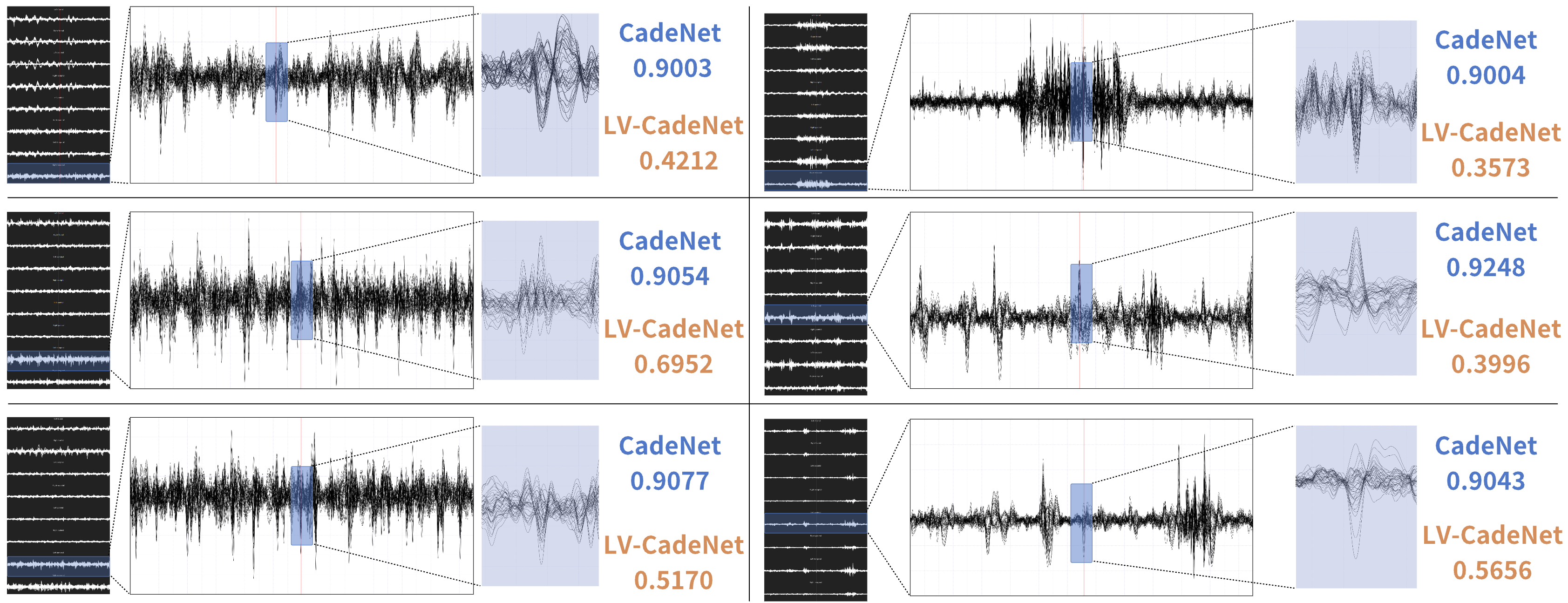
Figure 6: Six exemplary signals showcasing the integration of the long view input features enhanced spike detection performance. Each subfigure, from left to right, represents a 6s 306-channel MEG slice, a 6s 39-channel MEG slice, and a 384ms 39-channel MEG slice.

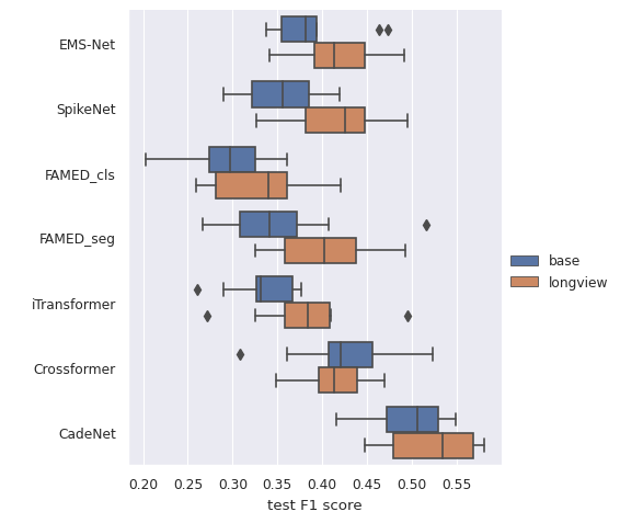
Figure 7: Ablation study on the long view input features we constructed.

3.2.3 Effect of long view input feature fusion

We conducted comparative experiments using long view feature fusion input $X$ on the optimal input lengths for all models, and the results are presented in Fig. 7. The experimental outcomes indicate that most models achieved superior results with the integration of long view features compared to their respective baselines. The average performance improvement is 3.39%, and the median improvement is 3.52% evaluated by F1 score. This suggests that our long view feature construction approach is not only a part of the CadeNet model framework but also a universally applicable technique in the task of spike detection.

Integrating long view input features into the CadeNet network has led to a 2.53% enhancement in performance, a figure that, while modest in comparison to the average improvement, still underscores the powerful feature extraction prowess of our network. Remarkably, this enhancement is observed despite the network’s already superior performance prior to the inclusion of these long view inputs. Six representative false positive instances are depicted in Fig. 6. In these cases, CadeNet falls short in providing accurate predictions, whereas LV-CadeNet successfully achieves this due to its enhanced capability in capturing the significance of long view spike patterns. Additionally, clinicians typically avoid conducting dipole analysis on waveforms that lack sufficient significance, as these are often heavily obscured by background noise or represent non-epileptic spikes. However, it poses a significant challenge for models to accurately assess the significance of waves when dealing with input spanning a short durations. By integrating the significance information of the signal over an extended time frame with the short-duration signal segments, via the normalization of morphological features across a broad FOV, our model acquires a visual perspective aligned with human cognitive perception.

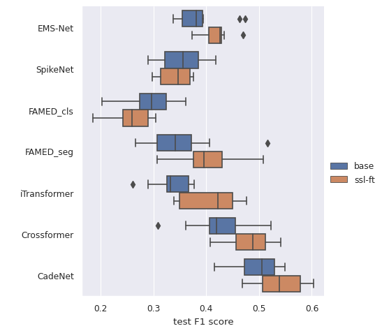
Figure 8: Performance comparison of all models with and without the semi-supervised learning scheme.

3.2.4 Effect of the semi-supervised learning scheme

We have conducted semi-supervised fine-tuning on all models, resulting in an average performance improvement of 2.97% and a median improvement of 4.26% as evaluated by the F1 score. Compared to those without semi-supervised fine-tuning, the performance of the segmentation models has significantly improved, while the impact on the classification models is uncertain. We believe this is because the segmentation models have a much larger sample size of predicted outputs than the classification models, which maintains better loss stability in the KL-divergence distillation method designed for semi-supervised fine-tuning in this paper. Furthermore, the application of the semi-supervised fine-tuning approach results in notable performance enhancements for iTransformer, Crossformer, and CadeNet, with respective improvements of 7.32%, 6.01%, and 4.26%. A shared characteristic of these methods is their reliance on attention mechanism-based feature extraction specifically targeting spatial features. This suggests that augmenting the training data size for transformer-based models is particularly effective in driving performance gains.

4 Conclusion

In this study, we introduce LV-CadeNet, an innovative framework for MEG spike detection that leverages our newly developed long view input features. This framework effectively captures both temporal and spatial characteristics through our convolution-attention encoder-decoder network. Additionally, we have enhanced the training process with data augmentation and semi-supervised learning for model fine-tuning. The application of LV-CadeNet on a real-world clinical dataset, encompassing data from 26 patients, has markedly enhanced the performance of automated MEG spike detection. In the future work, we will evaluate our framework on clinical data from multiple centers, and optimize the framework accordingly.

References

- [1] G. L. Barkley and C. Baumgartner, “MEG and EEG in epilepsy,” Journal of clinical neurophysiology, vol. 20, no. 3, pp. 163–178, 2003.
- [2] R. C. Burgess, “MEG for greater sensitivity and more precise localization in epilepsy,” Neuroimaging Clinics, vol. 30, no. 2, pp. 145–158, 2020.
- [3] F. E. Abd El-Samie, T. N. Alotaiby, M. I. Khalid, S. A. Alshebeili, and S. A. Aldosari, “A review of EEG and MEG epileptic spike detection algorithms,” IEEE Access, p. 60673–60688, Jan 2018.
- [4] J. Zhang, J. Zou, M. Wang, L. Chen, C. Wang, and G. Wang, “Automatic detection of interictal epileptiform discharges based on time-series sequence merging method,” Neurocomputing, vol. 110, pp. 35–43, 2013.
- [5] M. Dümpelmann and C. Elger, “Visual and automatic investigation of epileptiform spikes in intracranial EEG recordings,” Epilepsia, vol. 40, no. 3, pp. 275–285, 1999.
- [6] M. Perreau Guimaraes, D. K. Wong, E. T. Uy, L. Grosenick, and P. Suppes, “Single-trial classification of MEG recordings,” IEEE Transactions on Biomedical Engineering, vol. 54, no. 3, pp. 436–443, 2007.
- [7] L. Zheng, P. Liao, S. Luo, J. Sheng, P. Teng, G. Luan, and J.-H. Gao, “EMS-Net: A deep learning method for autodetecting epileptic Magnetoencephalography spikes,” IEEE Transactions on Medical Imaging, p. 1833–1844, Jun 2020.
- [8] R. Hirano, T. Emura, O. Nakata, T. Nakashima, M. Asai, K. Kagitani-Shimono, H. Kishima, and M. Hirata, “Fully-Automated spike detection and dipole analysis of epileptic MEG using deep learning,” IEEE Transactions on Medical Imaging, p. 2879–2890, Oct 2022.
- [9] J. Jing, H. Sun, J. A. Kim, A. Herlopian, I. Karakis, M. Ng, J. J. Halford, D. Maus, F. Chan, M. Dolatshahi, C. Muniz, C. Chu, V. Sacca, J. Pathmanathan, W. Ge, J. Dauwels, A. Lam, A. J. Cole, S. S. Cash, and M. B. Westover, “Development of Expert-Level Automated Detection of Epileptiform Discharges During Electroencephalogram Interpretation,” JAMA Neurology, p. 103, Jan 2020.
- [10] Z. Xu, T. Wang, J. Cao, Z. Bao, T. Jiang, and F. Gao, “BECT Spike Detection Based on Novel EEG Sequence Features and LSTM Algorithms,” IEEE Transactions on Neural Systems and Rehabilitation Engineering, p. 1734–1743, Jan 2021.
- [11] A. H. Mohammed, M. Cabrerizo, A. Pinzon, I. Yaylali, P. Jayakar, and M. Adjouadi, “Graph Neural Networks in EEG Spike Detection,” SSRN Electronic Journal, Nov 2022.
- [12] K. Fukumori, N. Yoshida, H. Sugano, M. Nakajima, and T. Tanaka, “Satelight: Self-attention-based model for epileptic spike detection from multi-electrode EEG.” Journal of Neural Engineering, p. 055007, Oct 2022.
- [13] S. Bagchi and D. R. Bathula, “EEG-ConvTransformer for single-trial EEG-based visual stimulus classification,” Pattern Recognition: The Journal of the Pattern Recognition Society, p. 129, 2022.
- [14] N. Networks, Z. Ming, D. Chen, T. Gao, Y. Tang, W. Tu, and J. Chen, “V2IED: Dual-view learning framework for detecting events of interictal epileptiform discharges.”
- [15] R. Nowak, M. Santiuste, and A. Russi, “Toward a definition of MEG spike: Parametric description of spikes recorded simultaneously by MEG and depth electrodes,” Seizure, p. 652–655, Nov 2009.
- [16] C. Laohathai, J. S. Ebersole, J. C. Mosher, A. I. Bagić, A. Sumida, G. Von Allmen, and M. E. Funke, “Practical Fundamentals of Clinical MEG Interpretation in Epilepsy,” Frontiers in Neurology, Oct 2021.
- [17] M. A. Kural, L. Duez, V. Sejer Hansen, P. G. Larsson, S. Rampp, R. Schulz, H. Tankisi, R. Wennberg, B. M. Bibby, M. Scherg, and S. Beniczky, “Criteria for defining interictal epileptiform discharges in EEG,” Neurology, May 2020.
- [18] S. Taulu and J. Simola, “Spatiotemporal signal space separation method for rejecting nearby interference in MEG measurements,” Physics in Medicine & Biology, vol. 51, no. 7, p. 1759, 2006.
- [19] W. Cui, M. Cao, X. Wang, L. Zheng, Z. Cen, P. Teng, G. Luan, and J.-H. Gao, “EMHapp: a pipeline for the automatic detection, localization and visualization of epileptic magnetoencephalographic high-frequency oscillations,” Journal of Neural Engineering, p. 055009, Oct 2022.
- [20] S. Ioffe and C. Szegedy, “Batch Normalization: Accelerating Deep Network Training by Reducing Internal Covariate Shift,” arXiv: Learning, Feb 2015.
- [21] D. Hendrycks and K. Gimpel, “Gaussian Error Linear Units (GELUs),” Cornell University - arXiv,Cornell University - arXiv, Jun 2016.
- [22] A. Vaswani, N. Shazeer, N. Parmar, J. Uszkoreit, L. Jones, A. Gomez, L. Kaiser, and I. Polosukhin, “Attention is All you Need,” Neural Information Processing Systems,Neural Information Processing Systems, Jun 2017.
- [23] N. Srivastava, G. Hinton, A. Krizhevsky, I. Sutskever, and R. Salakhutdinov, “Dropout: a simple way to prevent neural networks from overfitting,” Journal of Machine Learning Research,Journal of Machine Learning Research, Jan 2014.
- [24] W. Shi, J. Caballero, F. Huszár, J. Totz, A. P. Aitken, R. Bishop, D. Rueckert, and Z. Wang, “Real-time single image and video super-resolution using an efficient sub-pixel convolutional neural network,” in Proceedings of the IEEE conference on computer vision and pattern recognition, 2016, pp. 1874–1883.
- [25] C. Szegedy, V. Vanhoucke, S. Ioffe, J. Shlens, and Z. Wojna, “Rethinking the Inception Architecture for Computer Vision,” in 2016 IEEE Conference on Computer Vision and Pattern Recognition (CVPR), Jun 2016.
- [26] Y. Ouali, C. Hudelot, and M. Tami, “An Overview of Deep Semi-Supervised Learning,” arXiv: Learning, Jun 2020.
- [27] Q. Xie, M.-T. Luong, E. Hovy, and Q. V. Le, “Self-Training With Noisy Student Improves ImageNet Classification,” in 2020 IEEE/CVF Conference on Computer Vision and Pattern Recognition (CVPR), Jun 2020.
- [28] G. Hinton, O. Vinyals, and J. Dean, “Distilling the Knowledge in a Neural Network,” Computer Science, vol. 14, no. 7, pp. 38–39, 2015.
- [29] W. Skrandies, “Global field power and topographic similarity,” Brain Topography, p. 137–141, Jan 1990.
- [30] A. Tarvainen and H. Valpola, “Mean teachers are better role models: Weight-averaged consistency targets improve semi-supervised deep learning results.” International Conference on Learning Representations,International Conference on Learning Representations, Jan 2017.
- [31] A. Neubeck and L. Van Gool, “Efficient Non-Maximum Suppression,” in 18th International Conference on Pattern Recognition (ICPR’06), vol. 3, 2006, pp. 850–855.
- [32] D. Van ’t Ent, I. Manshanden, P. Ossenblok, D. Velis, J. de Munck, J. Verbunt, and F. Lopes da Silva, “Spike cluster analysis in neocortical localization related epilepsy yields clinically significant equivalent source localization results in magnetoencephalogram (MEG),” Clinical Neurophysiology, vol. 114, no. 10, pp. 1948–1962, 2003.
- [33] Y. Liu, T. Hu, H. Zhang, H. Wu, S. Wang, and M. Long, “ITRANSFORMER: INVERTED TRANSFORMERS ARE EFFECTIVE FOR TIME SERIES FORECASTING.”
- [34] Y. Zhang and J. Yan, “Crossformer: Transformer Utilizing Cross-Dimension Dependency for Multivariate Time Series Forecasting,” in International Conference on Learning Representations, 2023.
- [35] R. Li, W. Liu, L. Yang, S. Sun, W. Hu, F. Zhang, and W. Li, “DeepUNet: A deep fully convolutional network for pixel-level sea-land segmentation,” IEEE journal of selected topics in applied earth observations and remote sensing, vol. 11, no. 11, pp. 3954–3962, 2018.