Late-time tails in nonlinear evolutions of merging black holes
Abstract
We uncover late-time gravitational-wave tails in fully nonlinear 3+1 dimensional numerical relativity simulations of merging black holes, using the highly accurate SpEC code. We achieve this result by exploiting the strong magnification of late-time tails due to binary eccentricity, recently observed in perturbative evolutions, and showcase here the tail presence in head-on configurations for several mass ratios close to unity. We validate the result through a large battery of numerical tests and detailed comparison with perturbative evolutions, which display striking agreement with full nonlinear ones. Our results offer yet another confirmation of the highly predictive power of black hole perturbation theory in the presence of a source, even when applied to nonlinear solutions. The late-time tail signal is much more prominent than anticipated until recently, and possibly within reach of gravitational-wave detectors measurements, unlocking observational investigations of an additional set of general relativistic predictions on the long-range gravitational dynamics.
Introduction. In the last few decades, the merger dynamics and subsequent relaxation regime (quasinormal “ringing”) of compact binaries with comparable-masses have been the subject of considerable modeling efforts, chiefly enabled by fully nonlinear numerical relativity (NR) evolutions [1, 2, 3, 4]. Gravitational-wave (GW) observations of coalescing black hole (BH) binaries [5, 6, 7, 8], granting an unprecedented opportunity of accessing the highly nonlinear regime of dynamical spacetimes, were the main driver for these efforts. In contrast, the subsequent late-time dynamics received much less attention from the physics community, partly because its signatures were thought to be out of reach of foreseeable experimental efforts.
BH perturbation theory [9] predicts that the dominant late-time effect in the relaxation of compact objects is a power-law contribution (“tail”), both in spherical symmetry [10, 11, 12, 13, 14, 15, 16, 17, 18, 19, 20, 21, 22] and axisymmetry [23, 24, 25, 26, 27, 28, 29, 30, 31, 32, 33, 34, 35, 36, 37, 38]. For instance, at future null infinity (), metric perturbations of a Schwarzschild BH decay with the leading-order power-law , with the retarded time and the waveform multipole.111An especially clear discussion of the spherically symmetric case can be found in Refs. [16, 18], and Chapter 12 of Ref. [39]. Tails constitute a clean probe of the long-range structure of dynamical spacetimes and allow for distinct predictions of the relaxation of compact object within GR [25]. Even more interestingly, as shown in [40] and discussed below, source-driven tails at intermediate times bear direct imprints of the strong-field binary dynamics. So far, late-time tails have only been studied numerically in a perturbative framework [12, 41, 24, 21, 38, 42, 40, 43], but never observed in nonlinear NR simulations of comparable-mass BH mergers. This was mostly due to the very high accuracy required to unveil them, together with the need for solid control over boundary and initial data (ID) effects. Here we present the first robust extraction of late-time tail terms from fully nonlinear NR simulations of comparable-mass BH binaries.
Characterising tail effects in numerical simulations is challenging, because excitations of quasinormal-modes (QNM) can take a long time to decay [38]. Hence, to identify tail contributions we must look for them in a regime where QNMs are short-lived, and the tail amplitude is large. The first is easy to achieve by targeting remnant BHs with small angular momentum (shorter relaxation time). The second condition is harder to obtain, because we do not know a-priori the dependence of the tail amplitude on the binary’s initial conditions. Recently, some of us [42] found through effective-one-body (EOB) [44, 45, 46] calculations in the small-mass-ratio limit, that the binary eccentricity induces a strong enhancement of the tail amplitude. Tails in perturbative radial infalls, with a similar source-driven setup that we employ, were computed in e. g. [47] and for the first time at in [48]. The mechanism behind this enhancement, and whether its explanation necessitates a modification to Price’s law were initially unknown. In [40] some of us subsequently constructed an analytical model, that accurately describes the source-driven tail behavior in test-particle evolutions (for a given trajectory). The model shows how the simple picture of a single “Price tail” needs to be replaced by a superposition of a large number of inverse power-law components giving rise to a long slowly-decaying transient (see also [43]). A key prediction of the model is that the tail amplitude reaches its maximum for radial infalls, hence in this work we restrict to head-on collisions. These analytical predictions, together with the considerations presented in [49, 50], equip us with the necessary understanding of ID and boundary effects to attempt extracting a tail signal in nonlinear evolution, and constitute the required semi-analytical tool to verify the robustness of numerical evolutions.
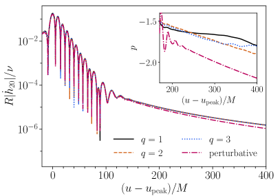
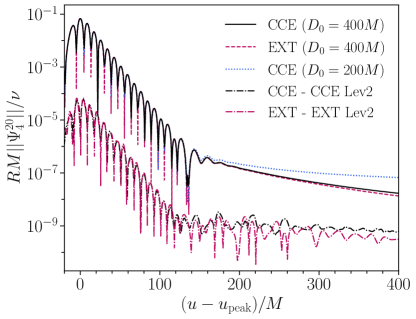
Exploiting the very high accuracy of the SpEC code [51], we demonstrate the extraction of tail effects in fully nonlinear 3+1 evolutions, displayed in Fig. 1. The figure shows the amplitude of the GW news quadrupolar mode extrapolated to , for several head-on binary simulations with mass ratios close to unity. Around after the peak, the amplitude transitions from an exponentially damped quasinormal-driven regime to a slowly-decaying non-oscillatory behaviour. The result aligns remarkably well with perturbative linear evolutions of an infalling test particle with compatible ID, further validating the numerical computation and pointing towards a suppression of nonlinear corrections [52].
Below, we report on the numerical methods employed both in the nonlinear and perturbative cases.
We discuss in more detail the results obtained, their interpretation, and possible nonlinear effects behind the subtle differences between linear and nonlinear evolutions.
We conclude summarising open questions and future detectability avenues for tail signals.
In the End Matter we give further details of the linearised analytical computation, and present a series of tests to confirm the robustness of our numerical results.
Conventions. We use geometric units . The GW strain is decomposed in spin-weight spherical harmonics modes, . To avoid memory contributions or gauge effects that could spoil tail extraction, entering as a constant offset at late times, we focus on the GW news function . Modes beyond the quadrupolar are subdominant, hence we are going to focus on . Exploiting the cylindrical symmetry of the problem, we present all results in a frame [53] in which the two BHs collide along the -axis and hence is the only non-zero waveform multipole. At asymptotically late-times, it holds: , with for Schwarzschild BHs. Hence it is convenient to define a “tail exponent” as
| (1) |
so that at late times.
With we indicate the Christodoulou masses [54]
of the individual black holes at the relaxation time of the
simulation (i.e., when the high-frequency oscillations in the Christodoulou masses have settled down), is the total Christodoulou mass of the system, the symmetric mass ratio, and the binary mass ratio.
The time axis is constructed by setting at the peak of , and is quoted in units of .
The tortoise coordinate in perturbative evolutions is , with the standard Schwarzschild coordinate.
We indicate the distance between the binary and the observer with .
Numerical methods. We generate non-linear evolutions of head-on collisions with the SpEC code [55, 56, 57, 58, 51], whose methods are summarised in [59, 60]. The ID [61, 62, 63, 64] are constructed using the extended conformal thin sandwich equations [65] and the evolution is carried out with the generalized harmonic formulation [66, 67]. Standard SpEC runs stop at a retarded time of after merger, which is typically enough to only resolve the quasinormal ringdown. In order to capture the late-time waveform behavior, here we carry out simulations with much longer post-merger components, stopping at retarded time after merger.
We compare these NR waveforms with linear perturbative waveforms of radial infalls towards a Schwarzschild BH, numerically computed using the RWZHyp code [68, 69]. We solve for the Regge-Wheeler/Zerilli equations, governing the evolution in time of gauge invariant quantities
| (2) |
These master variables encode the odd/even metric degrees of freedom at the linear level [47]. In the linear evolutions, we set null ID , as the perturbations are driven by the presence of the source . The latter is evaluated on the infalling test-particle’s trajectory. We refer to [40] for additional details and the source explicit expression. For radial infalls with null ID, the odd sector is identically zero, hence in what follows we drop the superscript. Following an EOB-inspired approach, we compute the particle’s trajectory solving the associated Hamiltonian equations of motion (see [42] for the explicit expressions), where dissipative effects linked to the GW emission are taken into account by including a radiation reaction force [47, 46]. Such a force was computed, for generic orbits by means of a PN-based, EOB-resummed analytical expansion [70, 71] for the fluxes of energy and angular momentum observed at infinity, and were shown to be consistent with the corresponding numerical quantities in Ref. [72]. Note that, due to the short time-scale of our dynamics, the inclusion of the radiation reaction force has a small impact on the evolution.
At large distances, the master function is related to the linearized strain’s spin weight spherical harmonic modes through [73]
| (3) |
Moreover, the source term is linearly proportional to the mass ratio, that in the test-particle limit is equivalent to the symmetric mass ratio, so . To compare perturbative waveforms with NR comparable-mass results, we will thus always rescale the perturbative results by . The NR waveforms are also rescaled with their symmetric mass-ratio.
To compare full NR results against perturbative test-mass limit ones, we initialise the two systems with compatible ID.
We only consider non-spinning black holes.
The SXS simulation ID are given by setting the angular momentum to
zero and by imposing that the Arnowitt-Deser-Misner (ADM) energy
is equal to the total rest mass of the system
within relative accuracy of , so that the two black holes are at rest at
infinite separation, and the initial binding energy is close to zero.
We generate equivalent test-mass data by imposing that the test-particle is at rest at infinity, i.e. by setting its initial energy equal to its mass.
Outer Boundary.
The SpEC code imposes data on the outer boundary, located on a sphere with radius , such that constraints are preserved [66], and the physical degrees of freedom are chosen assuming that there is no gravitational radiation entering the numerical domain [74, 75]. In curved spacetimes, however, a certain amount of radiation is always scattered back. Back-scattering, giving rise to wave propagation well within the light-cone, is precisely the mechanism responsible for tails generation [76, 77, 78, 79, 40], and a small would imply missing a significant fraction of such contribution. Hence, to capture the vast majority of the back-scattered radiation, we place the outer boundary exceptionally far away from the binary location (see Tab. 1).
Moreover, due to imperfect boundary conditions, when radiation reaches the boundary, a non-physical numerical artifact is generated, contaminating the signal with numerical noise. As pointed out in Refs. [49, 50], this contamination can alter the structure of tails. Therefore, to study the long-range and late-time tails contribution, it is important that our simulations remain causally disconnected from the boundary. To avoid such contamination, we chose to be large enough such that the boundary is never in causal contact with the extraction spheres for the entire evolution (see Table 1). This causal structure, our evolution domain, and the locations of finite-radius observers are visualized in Fig. 2. In the End Matter, in Table 2 we report the details of additional SpEC simulations in which there is causal contact between the boundary and the extraction spheres, clearly showing a strong impact on the behavior of the tail.
GW extraction. The RWZHyp software uses a numerical domain that is decomposed into two regions, a compact inner region and an outer hyperboloidal layer [80, 81, 82]. The inner region contains the particle trajectories and has a uniform grid in , ranging from to large a value of . The hyperboloidal layer, compactified over , is attached at the end of the inner region in order to bring into the computational domain. As a result, perturbative waveforms can be computed both at finite distances, in terms of the coordinate time , as well as at in terms of the retarded time .
In SpEC the GW information is extracted on spheres, whose radii are distributed in the interval and are held fixed across all simulations in this work, as opposed to standard SpEC runs in which their radii scale with . The extracted finite radius waveform data are extrapolated to by a standard polynomial fit using the method of [83] as implemented in the scri package [84, 85, 86, 87, 88].
We give additional details of the simulations in the End Matter, where we present convergence tests in terms of resolution, extrapolation methods, and initial separation, validating the robustness of our results. Furthermore we discuss results from waveform extraction by Cauchy-characteristic evolution.
Results.
| SXS identifier | ||||
|---|---|---|---|---|
| SXS:BBH:3991 | 1 | 100 | 4000 | 1600 |
| SXS:BBH:3997 | 2 | 100 | 4000 | 1600 |
| SXS:BBH:3998 | 3 | 100 | 4000 | 1600 |
| SXS:BBH:3994 | 1 | 100 | 8000 | 5600 |
| SXS:BBH:3995 | 1 | 200 | 8000 | 5600 |
| SXS:BBH:3996 | 1 | 400 | 8000 | 5600 |
In Table 1 we report the parameters of the simulations carried out with the above methods. Fig. 1 shows the resulting news function, normalized by the symmetric mass ratio, with respect to the retarded time . A first striking result from Fig. 1 concerns the dependence of the tail on the mass ratio. In fact, after mass-rescaling the waveforms appropriately, the comparable mass waveforms with different mass ratio are very similar (around the percent level), suggesting that finite mass ratio corrections do not play a significant role in the waveform generation, including the tail part.
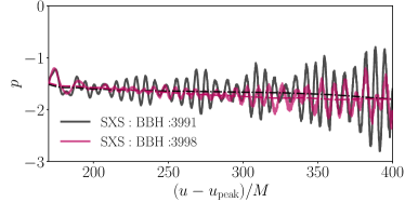
We also compute the tail exponent (Eq. (1)), reported in Fig. 1 inset. Its magnitude is much smaller than the asymptotic Price-law value (, for this multipole), towards which we would expect it to slowly converge [40]. Such decrease in exponent magnitude significantly boosts the tail amplitude at intermediate times. This result agrees with the analytical perturbative picture of Ref. [40], according to which tail emission is maximized for motion at large distances from the central BH, with small angular velocity. The additional numerical time derivative required for the exponent computation, combined with finite resolution, tends to introduce high-frequency noise. To compute the tail exponent at late-times we therefore apply a Savitzky-Golay filter [90] on the waveform to suppress high frequency oscillations. In the End Matter we compare the unfiltered tail exponent with respect to the one computed after applying the Savitzky-Golay filter, showcasing that our conclusions are not impacted by the filtering.
Even the test-mass perturbative case (similarly rescaled, and aligned minimising the post-peak mismatch) shows a remarkable agreement with the nonlinear evolutions, displaying the same slowly-decaying behaviour and an identical overall morphology. Such results confirm that the tail is primarily generated by the source term. This aligns with previous findings, which showcased how test-particle perturbative evolutions proved to be a remarkably accurate tool for the modelling of inspiral-merger-ringdown waveforms [47, 46, 91]. Somewhat surprisingly though, this framework provides quantitatively accurate predictions even for comparable mass systems [92, 93], as we confirm here. This is true even in the (a priori strong-field) merger stage, as notably depicted also in Fig. 2 of [94].
However, in Fig. 1 above there is visibly growing mismatch as the tail evolves, with the nonlinear evolution displaying a slower decay with respect to the perturbative result.
This may be due to a variety of effects, including the presence of nonlinear tail components (computed in [52] for modes within second order perturbation theory, see also [95]), together with corrections due the finite mass-ratio or the time-dependent background nature in the nonlinear case [96, 97, 98, 99, 100].
Although the good agreement in the quasinormal-driven regime suggests the last two effects are likely small, the hereditary nature of tails implies that small differences in the evolution can accumulate and impart a larger effect.
Future avenues. We have uncovered late-time gravitational-wave tails in 3+1 nonlinear simulations of black holes collisions through the highly accurate SpEC code, robustly validating this result through a number of numerical tests. The waveforms display a remarkable agreement with perturbative results, a fact that deserves further scrutiny in future works.
Our results raise several interesting questions. On the modeling side, these include: What is the non-linear content of late-time tails? Can second-order tails explain the observed differences between linear and nonlinear evolutions? Or can these instead be accounted for by higher-order (self-force type) corrections to the trajectory or the dynamical background? Precision studies on this subject will benefit from longer simulations and the development of Cauchy Characteristic Matching techniques [101, 102, 103] or non-linear codes in hyperboloidal coordinates [104], to uncover the subtle role of nonlinearities.
On the observational side, the tail sensitivity to the long-range spacetime structure implies it might be used as a tool to detect “environmental” effects around binaries, such as those induced by dark matter halos, accretion disks, boson clouds, as well as a tertiary object. This could open up an entire new way of characterising non-vacuum spacetimes, as displayed e.g. in [105] and discussed in [52]. The impact of these configurations on tails will be the subject of future investigation. Observability studies will greatly benefit from the construction of analytical tail models for spinning remnants (akin to [40]), as spin might enhance tails even further [43].
The source-driven enhancement of the tail brings it much closer to the reach of upcoming GW observatories, hence our results open the possibility of observational tests of general relativistic predictions on the long-range structure of highly-curved spacetimes.
A detailed tail detectability study is the subject of ongoing investigations.
Acknowledgments.
M. De A. expresses her gratitude to Perimeter Institute for its kind hospitality during the final stages of the paper’s preparation.
M. De A. also thanks Sizheng Ma and Luis Lehner for stimulating discussions on the topic during the visit.
S.A. gratefully acknowledges the warm hospitality of the Niels Bohr Institute, where this work was initiated.
G.C. acknowledges funding from the European Union’s Horizon 2020 research and innovation program under the Marie Skłodowska-Curie grant agreement No. 847523 ‘INTERACTIONS’.
We acknowledge support from the Villum Investigator program by the VILLUM Foundation (grant no. VIL37766) and the DNRF Chair program (grant no. DNRF162) by the Danish National Research Foundation.
H.R.R. and V. C. acknowledge financial support provided under the European Union’s H2020 ERC Advanced Grant “Black holes: gravitational engines of discovery” grant agreement no. Gravitas–101052587.
Views and opinions expressed are however those of the authors only and do not necessarily reflect those of the European Union or the European Research Council. Neither the European Union nor the granting authority can be held responsible for them.
This project has received funding from the European Union’s Horizon 2020 research and innovation programme under the Marie Skłodowska-Curie grant agreement No 101007855 and No 101131233.
K.M. is supported by NASA through the NASA Hubble Fellowship grant #HST-HF2-51562.001-A awarded by the Space Telescope Science Institute, which is operated by the Association of Universities for Research in Astronomy, Incorporated, under NASA contract NAS5-26555.
S.A. acknowledges support from the Deutsche Forschungsgemeinschaft (DFG) project “GROOVHY”
(BE 6301/5-1 Projektnummer: 523180871).
L.C.S. acknowledges support from NSF CAREER Award PHY–2047382 and a Sloan Foundation Research Fellowship.
This material is based upon work supported by the National Science Foundation under Grants No. PHY-2407742, No. PHY-2207342, and No. OAC-2209655 at Cornell. Any opinions, findings, and conclusions or recommendations expressed in this material are those of the author(s) and do not necessarily reflect the views of the National Science Foundation. This work was supported by the Sherman Fairchild Foundation at Cornell.
This work was supported in part by the Sherman Fairchild Foundation and by NSF Grants No. PHY-2309211, No. PHY-2309231, and No. OAC-2209656 at Caltech.
Simulations have been carried out on the Frontera computing system
within the Texas Advanced Computing Center (TACC) grant PHY20018,
“Gravitational Waves from Compact Binaries: Computational
Contributions to LIGO”.
Software. The version of the RWZHyp code used bears the tag tails, on the rwzhyp_eccentric branch. The manuscript content has been derived using publicly available software: matplotlib [106], numpy [107], scipy [108] and sxs [109].
Data availability. SpEC simulation data will be made available in the SXS waveform catalog [89].
References
- Pretorius [2005] F. Pretorius, Evolution of binary black hole spacetimes, Phys. Rev. Lett. 95, 121101 (2005), arXiv:gr-qc/0507014 .
- Campanelli et al. [2006] M. Campanelli, C. O. Lousto, P. Marronetti, and Y. Zlochower, Accurate evolutions of orbiting black-hole binaries without excision, Phys. Rev. Lett. 96, 111101 (2006), arXiv:gr-qc/0511048 .
- Baker et al. [2006] J. G. Baker, J. Centrella, D.-I. Choi, M. Koppitz, and J. van Meter, Gravitational wave extraction from an inspiraling configuration of merging black holes, Phys. Rev. Lett. 96, 111102 (2006), arXiv:gr-qc/0511103 .
- Berti et al. [2007] E. Berti, V. Cardoso, J. A. Gonzalez, U. Sperhake, M. Hannam, S. Husa, and B. Bruegmann, Inspiral, merger and ringdown of unequal mass black hole binaries: A Multipolar analysis, Phys. Rev. D 76, 064034 (2007), arXiv:gr-qc/0703053 .
- Abbott et al. [2016] B. P. Abbott et al., Observation of Gravitational Waves from a Binary Black Hole Merger, Phys. Rev. Lett. 116, 061102 (2016).
- Aasi et al. [2015] J. Aasi et al. (LIGO Scientific Collaboration), Advanced LIGO, Classical Quantum Gravity 32, 074001 (2015), arXiv:1411.4547 [gr-qc] .
- Acernese et al. [2015] F. Acernese et al. (Virgo Collaboration), Advanced Virgo: a second-generation interferometric gravitational wave detector, Classical Quantum Gravity 32, 024001 (2015), arXiv:1408.3978 [gr-qc] .
- Akutsu et al. [2021] T. Akutsu et al. (KAGRA), Overview of KAGRA: Detector design and construction history, Progress of Theoretical and Experimental Physics 2021, 05A101 (2021), arXiv:2005.05574 [physics.ins-det] .
- DeWitt and Brehme [1960] B. S. DeWitt and R. W. Brehme, Radiation damping in a gravitational field, Annals of Physics 9, 220 (1960).
- Price [1972a] R. H. Price, Nonspherical perturbations of relativistic gravitational collapse. 1. Scalar and gravitational perturbations, Phys. Rev. D 5, 2419 (1972a).
- Price [1972b] R. H. Price, Nonspherical Perturbations of Relativistic Gravitational Collapse. II. Integer-Spin, Zero-Rest-Mass Fields, Phys. Rev. D 5, 2439 (1972b).
- Cunningham et al. [1978] C. T. Cunningham, R. H. Price, and V. Moncrief, Radiation from collapsing relativistic stars. I - Linearized odd-parity radiation, Astrophys. J. 224, 643 (1978).
- Gómez and Winicour [1992] R. Gómez and J. Winicour, Asymptotics of gravitational collapse of scalar waves, Journal of Mathematical Physics 33, 1445 (1992).
- Gundlach et al. [1994a] C. Gundlach, R. H. Price, and J. Pullin, Late time behavior of stellar collapse and explosions: 1. Linearized perturbations, Phys. Rev. D 49, 883 (1994a), arXiv:gr-qc/9307009 .
- Gundlach et al. [1994b] C. Gundlach, R. H. Price, and J. Pullin, Late time behavior of stellar collapse and explosions: 2. Nonlinear evolution, Phys. Rev. D 49, 890 (1994b), arXiv:gr-qc/9307010 .
- Leaver [1986] E. W. Leaver, Spectral decomposition of the perturbation response of the Schwarzschild geometry, Phys. Rev. D 34, 384 (1986).
- Ching et al. [1995] E. S. C. Ching, P. T. Leung, W. M. Suen, and K. Young, Late time tail of wave propagation on curved space-time, Phys. Rev. Lett. 74, 2414 (1995), arXiv:gr-qc/9410044 .
- Andersson [1997] N. Andersson, Evolving test fields in a black hole geometry, Phys. Rev. D 55, 468 (1997), arXiv:gr-qc/9607064 .
- Burko and Ori [1997] L. M. Burko and A. Ori, Late time evolution of nonlinear gravitational collapse, Phys. Rev. D 56, 7820 (1997), arXiv:gr-qc/9703067 .
- Barack [1999] L. Barack, Late time dynamics of scalar perturbations outside black holes. 2. Schwarzschild geometry, Phys. Rev. D 59, 044017 (1999), arXiv:gr-qc/9811028 .
- Bernuzzi et al. [2008] S. Bernuzzi, A. Nagar, and R. De Pietri, Dynamical excitation of space-time modes of compact objects, Phys. Rev. D 77, 044042 (2008), arXiv:0801.2090 [gr-qc] .
- Hod [2009] S. Hod, How pure is the tail of gravitational collapse?, Class. Quant. Grav. 26, 028001 (2009), arXiv:0902.0237 [gr-qc] .
- Krivan et al. [1996] W. Krivan, P. Laguna, and P. Papadopoulos, Dynamics of scalar fields in the background of rotating black holes, Phys. Rev. D 54, 4728 (1996), arXiv:gr-qc/9606003 .
- Krivan et al. [1997] W. Krivan, P. Laguna, P. Papadopoulos, and N. Andersson, Dynamics of perturbations of rotating black holes, Phys. Rev. D 56, 3395 (1997), arXiv:gr-qc/9702048 .
- Hod [2000a] S. Hod, The Radiative tail of realistic gravitational collapse, Phys. Rev. Lett. 84, 10 (2000a), arXiv:gr-qc/9907096 .
- Hod [2000b] S. Hod, Mode coupling in rotating gravitational collapse of a scalar field, Phys. Rev. D 61, 024033 (2000b), arXiv:gr-qc/9902072 .
- Barack and Ori [1999] L. Barack and A. Ori, Late time decay of scalar perturbations outside rotating black holes, Phys. Rev. Lett. 82, 4388 (1999), arXiv:gr-qc/9902082 .
- Ori [2000] A. Ori, Evolution of linear gravitational and electromagnetic perturbations inside a Kerr black hole, Phys. Rev. D 61, 024001 (2000).
- Krivan [1999] W. Krivan, Late time dynamics of scalar fields on rotating black hole backgrounds, Phys. Rev. D 60, 101501 (1999), arXiv:gr-qc/9907038 .
- Poisson [2002] E. Poisson, Radiative falloff of a scalar field in a weakly curved space-time without symmetries, Phys. Rev. D 66, 044008 (2002), arXiv:gr-qc/0205018 .
- Burko and Khanna [2003] L. M. Burko and G. Khanna, Radiative falloff in the background of rotating black hole, Phys. Rev. D 67, 081502 (2003), arXiv:gr-qc/0209107 .
- Burko and Khanna [2004] L. M. Burko and G. Khanna, Universality of massive scalar field late time tails in black hole space-times, Phys. Rev. D 70, 044018 (2004), arXiv:gr-qc/0403018 .
- Burko and Khanna [2009] L. M. Burko and G. Khanna, Late-time Kerr tails revisited, Class. Quant. Grav. 26, 015014 (2009), arXiv:0711.0960 [gr-qc] .
- Burko and Khanna [2011] L. M. Burko and G. Khanna, Late-time Kerr tails: Generic and non-generic initial data sets, ’up’ modes, and superposition, Class. Quant. Grav. 28, 025012 (2011), arXiv:1001.0541 [gr-qc] .
- Racz and Toth [2011] I. Racz and G. Z. Toth, Numerical investigation of the late-time Kerr tails, Class. Quant. Grav. 28, 195003 (2011), arXiv:1104.4199 [gr-qc] .
- Zenginoğlu et al. [2014] A. Zenginoğlu, G. Khanna, and L. M. Burko, Intermediate behavior of Kerr tails, Gen. Rel. Grav. 46, 1672 (2014), arXiv:1208.5839 [gr-qc] .
- Burko and Khanna [2014] L. M. Burko and G. Khanna, Mode coupling mechanism for late-time Kerr tails, Phys. Rev. D 89, 044037 (2014), arXiv:1312.5247 [gr-qc] .
- Harms et al. [2013] E. Harms, S. Bernuzzi, and B. Brügmann, Numerical solution of the 2+1 Teukolsky equation on a hyperboloidal and horizon penetrating foliation of Kerr and application to late-time decays, Class. Quant. Grav. 30, 115013 (2013), arXiv:1301.1591 [gr-qc] .
- Maggiore [2018] M. Maggiore, Gravitational Waves. Vol. 2 (Oxford University Press, 2018).
- De Amicis et al. [2024] M. De Amicis, S. Albanesi, and G. Carullo, Inspiral-inherited ringdown tails, Phys. Rev. D 110, 104005 (2024), arXiv:2406.17018 [gr-qc] .
- Price and Pullin [1994] R. H. Price and J. Pullin, Colliding black holes: The Close limit, Phys. Rev. Lett. 72, 3297 (1994), arXiv:gr-qc/9402039 .
- Albanesi et al. [2023] S. Albanesi, S. Bernuzzi, T. Damour, A. Nagar, and A. Placidi, Faithful effective-one-body waveform of small-mass-ratio coalescing black hole binaries: The eccentric, nonspinning case, Phys. Rev. D 108, 084037 (2023), arXiv:2305.19336 [gr-qc] .
- Islam et al. [2024] T. Islam, G. Faggioli, G. Khanna, S. E. Field, M. van de Meent, and A. Buonanno, Phenomenology and origin of late-time tails in eccentric binary black hole mergers (2024), arXiv:2407.04682 [gr-qc] .
- Buonanno and Damour [1999] A. Buonanno and T. Damour, Effective one-body approach to general relativistic two-body dynamics, Phys. Rev. D 59, 084006 (1999), arXiv:gr-qc/9811091 .
- Buonanno and Damour [2000] A. Buonanno and T. Damour, Transition from inspiral to plunge in binary black hole coalescences, Phys. Rev. D 62, 064015 (2000), arXiv:gr-qc/0001013 .
- Damour and Nagar [2007] T. Damour and A. Nagar, Faithful effective-one-body waveforms of small-mass-ratio coalescing black-hole binaries, Phys. Rev. D 76, 064028 (2007), arXiv:0705.2519 [gr-qc] .
- Nagar et al. [2007] A. Nagar, T. Damour, and A. Tartaglia, Binary black hole merger in the extreme mass ratio limit, Class. Quant. Grav. 24, S109 (2007), arXiv:gr-qc/0612096 .
- Bernuzzi et al. [2012] S. Bernuzzi, A. Nagar, and A. Zenginoglu, Horizon-absorption effects in coalescing black-hole binaries: An effective-one-body study of the non-spinning case, Phys. Rev. D 86, 104038 (2012), arXiv:1207.0769 [gr-qc] .
- Allen et al. [2004] E. W. Allen, E. Buckmiller, L. M. Burko, and R. H. Price, Radiation tails and boundary conditions for black hole evolutions, Phys. Rev. D 70, 044038 (2004), arXiv:gr-qc/0401092 .
- Dafermos and Rodnianski [2004] M. Dafermos and I. Rodnianski, A Note on boundary value problems for black hole evolutions, (2004), arXiv:gr-qc/0403034 .
- [51] https://www.black-holes.org/SpEC.html.
- Cardoso et al. [2024] V. Cardoso, G. Carullo, M. De Amicis, F. Duque, T. Katagiri, D. Pereniguez, J. Redondo-Yuste, T. F. M. Spieksma, and Z. Zhong, Hushing black holes: Tails in dynamical spacetimes, Phys. Rev. D 109, L121502 (2024), arXiv:2405.12290 [gr-qc] .
- Gualtieri et al. [2008] L. Gualtieri, E. Berti, V. Cardoso, and U. Sperhake, Transformation of the multipolar components of gravitational radiation under rotations and boosts, Phys. Rev. D 78, 044024 (2008), arXiv:0805.1017 [gr-qc] .
- Christodoulou and Ruffini [1971] D. Christodoulou and R. Ruffini, Reversible transformations of a charged black hole, Phys. Rev. D 4, 3552 (1971).
- Scheel et al. [2009] M. A. Scheel et al., High-accuracy waveforms for binary black hole inspiral, merger, and ringdown, Phys. Rev. D79, 024003 (2009), arXiv:0810.1767 [gr-qc] .
- Szilagyi et al. [2009] B. Szilagyi, L. Lindblom, and M. A. Scheel, Simulations of Binary Black Hole Mergers Using Spectral Methods, Phys. Rev. D80, 124010 (2009), arXiv:0909.3557 [gr-qc] .
- Hemberger et al. [2013] D. A. Hemberger, M. A. Scheel, L. E. Kidder, B. Szilágyi, G. Lovelace, N. W. Taylor, and S. A. Teukolsky, Dynamical Excision Boundaries in Spectral Evolutions of Binary Black Hole Spacetimes, Class. Quant. Grav. 30, 115001 (2013), arXiv:1211.6079 [gr-qc] .
- Ossokine et al. [2013] S. Ossokine, L. E. Kidder, and H. P. Pfeiffer, Precession-tracking coordinates for simulations of compact-object-binaries, Phys. Rev. D 88, 084031 (2013), arXiv:1304.3067 [gr-qc] .
- Mroué et al. [2013] A. H. Mroué, M. A. Scheel, B. Szilágyi, H. P. Pfeiffer, M. Boyle, D. A. Hemberger, L. E. Kidder, G. Lovelace, S. Ossokine, N. W. Taylor, A. i. e. i. f. Zenginoğlu, L. T. Buchman, T. Chu, E. Foley, M. Giesler, R. Owen, and S. A. Teukolsky, Catalog of 174 binary black hole simulations for gravitational wave astronomy, Phys. Rev. Lett. 111, 241104 (2013), arXiv:gr-qc/0512093 [gr-qc] .
- Boyle et al. [2019] M. Boyle et al., The SXS Collaboration catalog of binary black hole simulations, Class. Quant. Grav. 36, 195006 (2019), arXiv:1904.04831 [gr-qc] .
- Lovelace et al. [2008] G. Lovelace, R. Owen, H. P. Pfeiffer, and T. Chu, Binary-black-hole initial data with nearly-extremal spins, Phys. Rev. D 78, 084017 (2008), arXiv:0805.4192 [gr-qc] .
- Buchman et al. [2012] L. T. Buchman, H. P. Pfeiffer, M. A. Scheel, and B. Szilagyi, Simulations of non-equal mass black hole binaries with spectral methods, Phys. Rev. D86, 084033 (2012), arXiv:1206.3015 [gr-qc] .
- Cook and Pfeiffer [2004] G. B. Cook and H. P. Pfeiffer, Excision boundary conditions for black hole initial data, Phys. Rev. D70, 104016 (2004), arXiv:gr-qc/0407078 [gr-qc] .
- Pfeiffer et al. [2003] H. P. Pfeiffer, L. E. Kidder, M. A. Scheel, and S. A. Teukolsky, A Multidomain spectral method for solving elliptic equations, Comput. Phys. Commun. 152, 253 (2003), arXiv:gr-qc/0202096 .
- Pfeiffer and York [2003] H. P. Pfeiffer and J. W. York, Extrinsic curvature and the einstein constraints, Phys. Rev. D 67, 044022 (2003), arXiv:gr-qc/0207095 [gr-qc] .
- Lindblom et al. [2006] L. Lindblom, M. A. Scheel, L. E. Kidder, R. Owen, and O. Rinne, A New generalized harmonic evolution system, Class.Quant.Grav. 23, S447 (2006), arXiv:gr-qc/0512093 [gr-qc] .
- Lindblom and Szilágyi [2009] L. Lindblom and B. Szilágyi, Improved gauge driver for the generalized harmonic einstein system, Physical Review D 80, 10.1103/physrevd.80.084019 (2009), arXiv:0904.4873 [gr-qc] .
- Bernuzzi and Nagar [2010] S. Bernuzzi and A. Nagar, Binary black hole merger in the extreme-mass-ratio limit: a multipolar analysis, Phys. Rev. D81, 084056 (2010), arXiv:1003.0597 [gr-qc] .
- Bernuzzi et al. [2011] S. Bernuzzi, A. Nagar, and A. Zenginoglu, Binary black hole coalescence in the large-mass-ratio limit: the hyperboloidal layer method and waveforms at null infinity, Phys.Rev. D84, 084026 (2011), arXiv:1107.5402 [gr-qc] .
- Bini and Damour [2012] D. Bini and T. Damour, Gravitational radiation reaction along general orbits in the effective one-body formalism, Phys. Rev. D 86, 124012 (2012), arXiv:1210.2834 [gr-qc] .
- Chiaramello and Nagar [2020] D. Chiaramello and A. Nagar, Faithful analytical effective-one-body waveform model for spin-aligned, moderately eccentric, coalescing black hole binaries, Phys. Rev. D 101, 101501 (2020), arXiv:2001.11736 [gr-qc] .
- Albanesi et al. [2021] S. Albanesi, A. Nagar, and S. Bernuzzi, Effective one-body model for extreme-mass-ratio spinning binaries on eccentric equatorial orbits: Testing radiation reaction and waveform, Phys. Rev. D 104, 024067 (2021), arXiv:2104.10559 [gr-qc] .
- Nagar and Rezzolla [2005] A. Nagar and L. Rezzolla, Gauge-invariant non-spherical metric perturbations of Schwarzschild black-hole spacetimes, Class. Quant. Grav. 22, R167 (2005), [Erratum: Class.Quant.Grav. 23, 4297 (2006)], arXiv:gr-qc/0502064 .
- Rinne [2006] O. Rinne, Stable radiation-controlling boundary conditions for the generalized harmonic einstein equations, Classical and Quantum Gravity 23, 6275 (2006), arXiv:gr-qc/0606053 [gr-qc] .
- Rinne et al. [2007] O. Rinne, L. Lindblom, and M. A. Scheel, Testing outer boundary treatments for the einstein equations, Classical and Quantum Gravity 24, 4053 (2007), arXiv:0704.0782 [gr-qc] .
- Blanchet and Damour [1992] L. Blanchet and T. Damour, Hereditary effects in gravitational radiation, Phys. Rev. D 46, 4304 (1992).
- Blanchet and Schaefer [1993] L. Blanchet and G. Schaefer, Gravitational wave tails and binary star systems, Class. Quant. Grav. 10, 2699 (1993).
- Poisson [1993] E. Poisson, Gravitational radiation from a particle in circular orbit around a black hole. 1: Analytical results for the nonrotating case, Phys. Rev. D 47, 1497 (1993).
- Poisson and Sasaki [1995] E. Poisson and M. Sasaki, Gravitational radiation from a particle in circular orbit around a black hole. 5: Black hole absorption and tail corrections, Phys. Rev. D 51, 5753 (1995), arXiv:gr-qc/9412027 .
- Zenginoglu [2008a] A. Zenginoglu, Hyperboloidal foliations and scri-fixing, Class. Quant. Grav. 25, 145002 (2008a), arXiv:0712.4333 [gr-qc] .
- Zenginoglu [2010] A. Zenginoglu, Asymptotics of black hole perturbations, Class. Quant. Grav. 27, 045015 (2010), arXiv:0911.2450 [gr-qc] .
- Zenginoglu [2011] A. Zenginoglu, Hyperboloidal layers for hyperbolic equations on unbounded domains, J. Comput. Phys. 230, 2286 (2011), arXiv:1008.3809 [math.NA] .
- Iozzo et al. [2021] D. A. B. Iozzo, M. Boyle, N. Deppe, J. Moxon, M. A. Scheel, L. E. Kidder, H. P. Pfeiffer, and S. A. Teukolsky, Extending gravitational wave extraction using weyl characteristic fields, Phys. Rev. D 103, 024039 (2021), arXiv:2010.15200 [gr-qc] .
- Boyle et al. [2020] M. Boyle, D. Iozzo, and L. C. Stein, moble/scri: v1.2, 10.5281/zenodo.4041972 (2020).
- [85] The scri package, https://github.com/sxs-collaboration/scri.
- Boyle [2013] M. Boyle, Angular velocity of gravitational radiation from precessing binaries and the corotating frame, Phys. Rev. D 87, 104006 (2013).
- Boyle et al. [2014] M. Boyle, L. E. Kidder, S. Ossokine, and H. P. Pfeiffer, Gravitational-wave modes from precessing black-hole binaries (2014), arXiv:1409.4431 [gr-qc] .
- Boyle [2016] M. Boyle, Transformations of asymptotic gravitational-wave data, Phys. Rev. D 93, 084031 (2016).
- [89] Sxs waveform catalog, http://www.black-holes.org/waveforms.
- Savitzky and Golay [1964] A. Savitzky and M. J. E. Golay, Smoothing and differentiation of data by simplified least squares procedures, Analytical Chemistry 36, 1627 (1964).
- Barausse et al. [2012] E. Barausse, A. Buonanno, S. A. Hughes, G. Khanna, S. O’Sullivan, and Y. Pan, Modeling multipolar gravitational-wave emission from small mass-ratio mergers, Phys. Rev. D 85, 024046 (2012), arXiv:1110.3081 [gr-qc] .
- Wardell et al. [2023] B. Wardell, A. Pound, N. Warburton, J. Miller, L. Durkan, and A. Le Tiec, Gravitational Waveforms for Compact Binaries from Second-Order Self-Force Theory, Phys. Rev. Lett. 130, 241402 (2023), arXiv:2112.12265 [gr-qc] .
- Islam and Khanna [2023] T. Islam and G. Khanna, Interplay between numerical relativity and perturbation theory: Finite size effects, Phys. Rev. D 108, 044012 (2023), arXiv:2306.08767 [gr-qc] .
- Nagar et al. [2022] A. Nagar, J. Healy, C. O. Lousto, S. Bernuzzi, and A. Albertini, Numerical-relativity validation of effective-one-body waveforms in the intermediate-mass-ratio regime, Phys. Rev. D 105, 124061 (2022), arXiv:2202.05643 [gr-qc] .
- Okuzumi et al. [2008] S. Okuzumi, K. Ioka, and M.-a. Sakagami, Possible Discovery of Nonlinear Tail and Quasinormal Modes in Black Hole Ringdown, Phys. Rev. D 77, 124018 (2008), arXiv:0803.0501 [gr-qc] .
- Sberna et al. [2022] L. Sberna, P. Bosch, W. E. East, S. R. Green, and L. Lehner, Nonlinear effects in the black hole ringdown: Absorption-induced mode excitation, Phys. Rev. D 105, 064046 (2022), arXiv:2112.11168 [gr-qc] .
- Redondo-Yuste et al. [2024] J. Redondo-Yuste, D. Pereñiguez, and V. Cardoso, Ringdown of a dynamical spacetime, Phys. Rev. D 109, 044048 (2024), arXiv:2312.04633 [gr-qc] .
- Zhu et al. [2024] H. Zhu et al., Imprints of Changing Mass and Spin on Black Hole Ringdown, (2024), arXiv:2404.12424 [gr-qc] .
- May et al. [2024] T. May, S. Ma, J. L. Ripley, and W. E. East, Nonlinear effect of absorption on the ringdown of a spinning black hole, Phys. Rev. D 110, 084034 (2024), arXiv:2405.18303 [gr-qc] .
- Capuano et al. [2024] L. Capuano, L. Santoni, and E. Barausse, Perturbations of the Vaidya metric in the frequency domain: Quasinormal modes and tidal response, Phys. Rev. D 110, 084081 (2024), arXiv:2407.06009 [gr-qc] .
- Bishop et al. [1998] N. T. Bishop, R. Gomez, L. Lehner, B. Szilagyi, J. Winicour, and R. A. Isaacson, Cauchy characteristic matching, in Black Holes, Gravitational Radiation and the Universe: Essays in Honor of C.V. Vishveshwara, edited by B. R. Iyer and B. Bhawal (1998) pp. 383–408, arXiv:gr-qc/9801070 .
- Szilagyi [2000] B. Szilagyi, Cauchy characteristic matching in general relativity, Other thesis (2000), arXiv:gr-qc/0006091 .
- Ma et al. [2024] S. Ma et al., Fully relativistic three-dimensional Cauchy-characteristic matching for physical degrees of freedom, Phys. Rev. D 109, 124027 (2024), arXiv:2308.10361 [gr-qc] .
- Peterson et al. [2024] C. Peterson, S. Gautam, A. Vañó Viñuales, and D. Hilditch, Spherical Evolution of the Generalized Harmonic Gauge Formulation of General Relativity on Compactified Hyperboloidal Slices, (2024), arXiv:2409.02994 [gr-qc] .
- Spieksma et al. [2024] T. F. M. Spieksma, V. Cardoso, G. Carullo, M. Della Rocca, and F. Duque, Black hole spectroscopy in environments: detectability prospects, (2024), arXiv:2409.05950 [gr-qc] .
- Hunter [2007] J. D. Hunter, Matplotlib: A 2d graphics environment, Comput. Sci. Eng. 9, 90 (2007).
- Harris et al. [2020] C. R. Harris et al., Array programming with NumPy, Nature (London) 585, 357 (2020).
- Virtanen and others [2020] P. Virtanen et al., Scipy 1.0: Fundamental algorithms for scientific computing in python, Nature Methods 17, 261 (2020).
- Boyle and Scheel [2024] M. Boyle and M. Scheel, The sxs package (2024).
- Blanchet and Sathyaprakash [1995] L. Blanchet and B. S. Sathyaprakash, Detecting the tail effect in gravitational wave experiments, Phys. Rev. Lett. 74, 1067 (1995).
- Zenginoglu [2008b] A. Zenginoglu, A Hyperboloidal study of tail decay rates for scalar and Yang-Mills fields, Class. Quant. Grav. 25, 175013 (2008b), arXiv:0803.2018 [gr-qc] .
- Deppe et al. [2024] N. Deppe, W. Throwe, L. E. Kidder, N. L. Vu, K. C. Nelli, C. Armaza, M. S. Bonilla, F. Hébert, Y. Kim, P. Kumar, G. Lovelace, A. Macedo, J. Moxon, E. O’Shea, H. P. Pfeiffer, M. A. Scheel, S. A. Teukolsky, N. A. Wittek, et al., SpECTRE v2024.09.29, 10.5281/zenodo.13858965 (2024).
- Moxon et al. [2020] J. Moxon, M. A. Scheel, and S. A. Teukolsky, Improved Cauchy-characteristic evolution system for high-precision numerical relativity waveforms, Phys. Rev. D 102, 044052 (2020), arXiv:2007.01339 [gr-qc] .
- Moxon et al. [2023] J. Moxon, M. A. Scheel, S. A. Teukolsky, N. Deppe, N. Fischer, F. Hébert, L. E. Kidder, and W. Throwe, SpECTRE Cauchy-characteristic evolution system for rapid, precise waveform extraction, Phys. Rev. D 107, 064013 (2023), arXiv:2110.08635 [gr-qc] .
- Mitman et al. [2021] K. Mitman et al., Fixing the BMS frame of numerical relativity waveforms, Phys. Rev. D 104, 024051 (2021), arXiv:2105.02300 [gr-qc] .
- Magaña Zertuche et al. [2022] L. Magaña Zertuche et al., High precision ringdown modeling: Multimode fits and BMS frames, Phys. Rev. D 105, 104015 (2022), arXiv:2110.15922 [gr-qc] .
- Mitman et al. [2022] K. Mitman et al., Fixing the BMS frame of numerical relativity waveforms with BMS charges, Phys. Rev. D 106, 084029 (2022), arXiv:2208.04356 [gr-qc] .
- Mitman et al. [2024] K. Mitman et al., A review of gravitational memory and BMS frame fixing in numerical relativity, Class. Quant. Grav. 41, 223001 (2024), arXiv:2405.08868 [gr-qc] .
END MATTER
| SXS identifier | ||||
|---|---|---|---|---|
| SXS:BBH:3985 | 1 | 100 | 1300 | |
| SXS:BBH:3986 | 1 | 200 | 1300 | |
| SXS:BBH:3987 | 1 | 400 | 1300 | |
| SXS:BBH:3988 | 1 | 100 | 2300 | |
| SXS:BBH:3989 | 1 | 200 | 2300 | |
| SXS:BBH:3990 | 1 | 400 | 2300 | |
| SXS:BBH:3992 | 1 | 200 | 4000 | 1600 |
| SXS:BBH:3993 | 1 | 400 | 4000 | 1600 |
Impact of initial separation.
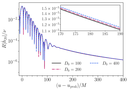
We investigate a sequence of NR simulations with and varying initial separation (with identifiers SXS:BBH:3994, SXS:BBH:3995 and SXS:BBH:3996 in Table 1).
If ID are set up consistently, the three evolutions should give close to indistinguishable results.
This is what Fig. 3 shows, with very small differences even when increasing the initial separation by a factor of four.
This confirms the robustness of our numerical evolutions.
However, in practice our ID at different separation will not be perfect (i.e. will not correctly capture the entire past binary history).
In this case, the tail amplitude is expected to increase with larger initial separation, since this enhances the overlap between the source and the tail propagator [40], consistently with tails hereditary nature [76, 77, 110, 78, 79].
Such increase is expected to be small if we are already at large enough separations, so that most of the relevant binary history is already captured.
This is confirmed by Fig. 3, showing a small increase of the tail amplitude when increasing the separation, another validation of the robustness of our results.
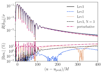
Resolution tests. In Fig. 4 we compare three different resolution levels (see [59, 60]), for the waveform of run SXS:BBH:3991 (see Tab. 1). We report the residuals relative to the highest resolution available, with smaller extrapolation order, , defined as
| (4) |
The tail properties are unchanged with increasing resolution, and differences between different resolution levels are too small to affect any of the considerations reported in the main text, including comparisons with perturbative waveforms.
Extrapolation procedure. We first recall known perturbative predictions to gain intuition on waveform extrapolation, and then test our results robustness with respect to the extrapolation procedure employed in the main text.
Perturbative picture – The tail in the strain observed at finite distances in terms of the coordinate time has an asymptotic behaviour [10, 16]. Hence, it is suppressed with respect to the signal observed at as a function of the retarded time , which is instead characterized by a decay . However, even when observed at finite distance, the late-time decay is characterized by a transient radiative tail , behaving as the one observed at [16]. This transient eventually leaves place to the term. In Ref. [111], ID-driven perturbative numerical simulations confirmed this picture, showing that a progressively longer transient appears as the observer is moved further away from the source. The physical interpretation is the following: tail signals are generated by the interaction of small frequency signals with the long-range, slow decay of the background. Smaller frequencies can probe larger scales and get more efficiently back-scattered. If the observer is located close to the BH, smaller frequencies cannot reach it and, as consequence, the observed tail is quenched.
Extrapolation of nonlinear simulations –
With this phenomenology in mind, we extrapolate the numerical
waveforms obtained from nonlinear evolutions to
using the SXS standard polynomial extrapolation procedure
of [83] as implemented in the
scri package [84, 85, 86, 87, 88], with polynomial order .
In Fig. 4 we also compare the results obtained with , showing that this does not alter our conclusions.
We choose extraction radii at large distances in the interval .
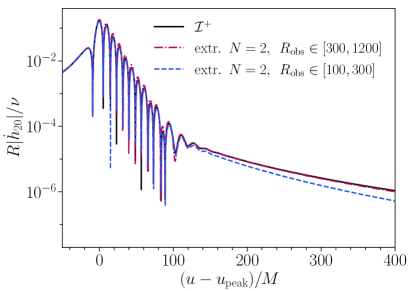
To gain intuition about whether our procedure leads to a correct extraction of tails, we perform a test on the perturbative waveforms computed with the RWZHyp code, where we can compare this result directly to waveforms computed at , see Fig. 5.
In particular, we compare two different extrapolations, computed considering and respectively.
As expected from our argument above, the extrapolation performed with closer to the BH yields a large mismatch with respect to the one computed at .
On the other hand, extrapolating with far enough from the BH, yields an extrapolation in excellent agreement with the tail computed at by means of the hyperboloidal layer.
The agreement slowly decreases in time; as expected, the extrapolated waveform undergoes a faster decay after the initial evolution.
Cauchy-characteristic Evolution. Apart from extrapolating waveforms to , we also investigate the use of Cauchy-characteristic evolution (CCE). We run SpECTRE code’s CCE module [112, 113, 114] on worldtubes with radii . Initial data for the first null hypersurface for each simulation was created using SpECTRE’s default ConformalFactor method. After running CCE, we mapped each system to the superrest frame of its remnant black hole 50M before the end of the simulation [115, 116, 117, 118].
In Fig. 6 we show the Newman-Penrose scalar extracted using CCE (with 222We use since this worldtube radius shows marginally better agreement with the extrapolated waveform. Larger worldtube radii tend to yield a slightly slower falloff. The reason behind this will be investigated in future work.) and extrapolation, for runs SXS:BBH:3995 and SXS:BBH:3996.
We also show the residual between the highest and next-highest resolutions for both the CCE and extrapolated waveforms.
As can be seen, while the CCE and extrapolated waveforms for seem to agree fairly well, for the CCE waveform has a much slower falloff than the extrapolated waveform.
We suspect that this inconsistency is likely due to the initial data in CCE.
In particular, with a shorter simulation, like SXS:BBH:3995 with , there is less time for the radiation due to unphysical initial data to propagate out of the system.
Consequently, the late-time tail behavior between the two simulations can take on fairly different structures.
We choose to work with extrapolated waveforms in the main text to mitigate this effect.
Understanding the impact of initial data on the tails of CCE waveforms will be the study of future work.
Waveform Filtering.
To reduce high-frequency numerical noise in the NR waveforms, we applied a Savitzky-Golay filter. The filter, acting on a sliding time window, is applied on the news amplitude in the interval . The two dominant noise frequency components are suppressed by applying the filter with a window length of and then , suppressing the modulations and the high frequency oscillations contaminating the news. The tail exponent is instead filtered with a -long window. The filter fits the data with a polynomial in the specified time window, then set as value of the filtered function the fit prediction at the center of the interval. We set the fitting function as linear, using scipy.signal.savgolfilter(data, windowlength=windowlength, polyorder=1).
In Fig. 7 we compare the filtered vs unfiltered tail exponent, for two exemplary SpEC simulations analyzed in this work. We report the simulations SXS:BBH:3991 and SXS:BBH:3998, which are evolved under the same initial data, but with different , to showcase how the result obtained is robust with respect to different binary initial data. Albeit contaminated by high-frequency noise, a clear decaying trend for the exponent is distinguishable.