How do uncertainties in galaxy formation physics impact field-level galaxy bias?

Abstract

Our ability to extract cosmological information from galaxy surveys is limited by uncertainties in the galaxy–dark matter halo relationship for a given galaxy population, which are governed by the intricacies of galaxy formation. To quantify these uncertainties, we examine quenched and star-forming galaxies using two distinct approaches to modeling galaxy formation: UniverseMachine, an empirical semi-analytic model, and the IllustrisTNG hydrodynamical simulation. We apply a second-order hybrid N-body perturbative bias expansion to each galaxy sample, enabling direct comparison of modeling approaches and revealing how uncertainties in galaxy formation and the galaxy–halo connection affect bias parameters and non-Poisson noise across number density and redshift. Notably, we find that quenched and star-forming galaxies occupy distinct parts of bias parameter space, and that the scatter induced from these entirely different galaxy formation models is small when conditioned on similar selections of galaxies. We also detect a signature of assembly bias in our samples; this leads to small but significant deviations from predictions of the analytic bias, while samples with assembly bias removed match these predictions well. This work indicates that galaxy samples from a spectrum of reasonable, physically motivated models for galaxy formation roughly spanning our current understanding give a relatively small range of field-level galaxy bias parameters and relations. We estimate a set of priors from this set of models that should be useful in extracting cosmological constraints from LRG- and ELG-like samples. Looking forward, this indicates that careful estimates of the range of impacts of galaxy formation, for a given sample and cosmological analysis, will be an essential ingredient for extracting the most precise cosmological information from current and future large galaxy surveys.

1 Introduction

Precision cosmology has entered a new era defined by an extraordinary wealth of data. Within the next decade, a multitude of ambitious new imaging surveys will see first light and map billions of galaxies. These include the Vera C. Rubin Observatory’s Legacy Survey of Space and Time (The LSST Dark Energy Science Collaboration et al., 2018; Ivezić et al., 2019), the Nancy Grace Roman Space Telescope (Akeson et al., 2019; Eifler et al., 2021), and the Spectro-Photometer for the History of the Universe, Epoch of Reionization and Ices Explorer (Doré et al., 2014, SPHEREx). Currently ongoing spectroscopic galaxy surveys, including the Dark Energy Spectroscopic Instrument (DESI Collaboration et al., 2016) and Euclid (Laureijs et al., 2011), are beginning to provide the first “Stage IV” cosmology constraints (Collaboration et al., 2024a, b). We can soon expect an explosion of rich, high signal-to-noise measurements of cosmological statistics at large and small scales due to the simultaneous increase in volume and density of galaxies cataloged by these surveys. Unfortunately, modeling uncertainties of galaxy and matter density fields in the non-linear regime limit our ability to fully extract data from these new measurements (e.g., Krause et al., 2017; MacCrann et al., 2020; Park et al., 2021).

One challenge of using these new survey data across their widest range of scales is improving the robustness of our theoretical models of galaxy clustering. Improving these models requires advancing our understanding of the galaxy–halo connection, which describes the statistical and physical relationship between luminous galaxies and the dark matter halos in which they are hosted. This is the key to deciphering the physics of galaxy formation, as there is currently a wide spectrum of acceptable modeling approaches to the galaxy–halo connection, ranging from ab initio models (e.g., hydrodynamical simulations) to more computationally tractable phenomenological models (e.g., halo occupation models). See Wechsler & Tinker (2018) for a broad overview of different approaches, and Somerville & Davé (2015) for a detailed review of ab initio models only. In this study, we present a way to quantify this uncertainty in the galaxy–halo connection using a methodology that employs the bias expansion to compare distinct galaxy formation models, as well as different populations of galaxies. Using this technique, we can place informative priors on the bias parameters (Barreira et al., 2020; Ivanov et al., 2024a; Akitsu, 2024) which can both improve constraints on cosmological parameters (Zhang et al., 2024; Ivanov et al., 2024c), alleviate projection effects (Carrilho et al., 2023), and inform which regimes the different galaxy formation models make similar or distinct predictions.

In its simplest form, the bias expansion states that galaxies are observable and biased tracers of dark matter (Kaiser, 1984; Mo & White, 1996), which means that there is a statistical relationship between their spatial distribution and the underlying distribution of dark matter. This relationship is known as galaxy bias (see Desjacques et al. 2018 for a review), and its exact form varies depending on the tracer population. On large scales, galaxy bias can be approximated by a single proportionality factor, the linear bias term. However, to accurately describe the way galaxies are distributed today, it is necessary to model the non-linear growth of structure. This can be achieved using the bias expansion, a perturbative parameterization of galaxy bias that encodes the response of galaxies to changes in large-scale structure, in combination with cosmological perturbation theory (PT), which models the clustering of dark matter in the Universe. For a comprehensive review of “standard” PT, and the reasons why it breaks down beyond large scales, we refer to Bernardeau et al. (2002).

Effective Field Theory (EFT) improves upon this approach with a more rigorous separation of small and large scales (Baumann et al., 2012; Carrasco et al., 2012). In doing so, it pushes the regime of accuracy of perturbation theory to smaller scales. However, by construction, EFT still breaks down at non-linear scales. To model scales beyond this, phenomenological models are required: these include the halo model, as well as full numerical solutions of the equations of structure formation, commonly in the form of N-body simulations. These simulations accurately capture the small-scale structure of the Universe, but their computational expense makes it extremely difficult to explore a wide cosmological parameter space. Modeling biased tracers of dark matter, such as galaxies, in such simulations is even more computationally expensive, motivating a technique known as Hybrid EFT (HEFT). This is a recent class of models that combines the small-scale accuracy of N-body simulations with the flexibility and generality of perturbation theories. HEFT operates in a Lagrangian coordinate system and uses the displacements from simulations rather than solving for them perturbatively as in traditional EFT (Modi et al., 2020; Kokron et al., 2021, 2022; Zennaro et al., 2023). This is the modeling approach we adopt in this paper, as HEFT has the capability to greatly improve cosmological constraints (Hadzhiyska et al., 2021a), and is starting to be actively used to obtain cosmological constraints from real data for the first time (Chen et al., 2024; Sailer et al., 2024).

The advent of complex bias models has presented a new challenge: the inclusion of additional nuisance parameters from the bias expansion can lead to effects in interpreting cosmological constraints in Bayesian analyses, known as prior volume effects. These are artifacts that occur when marginalizing the posterior over a highly dimensional parameter space, such that the estimated cosmological parameters are seemingly biased relative to their “true” value (Holm et al., 2023; Simon et al., 2023; Maus et al., 2023). This is especially a problem for EFT-based analyses, which can successfully describe mildly non-linear scales, but are governed by bias parameters that are often degenerate with cosmological parameters. Although there exist techniques that circumvent this effect (Donald-McCann et al., 2023; Zhao et al., 2024; Ried Guachalla et al., 2024), since this issue is partially driven by too-broad priors, one can instead use our knowledge of galaxy formation to determine which values of the nuisance parameters are physically allowed, and place informed priors on them to begin with. This reduces parameter space and improves computational feasibility; as degeneracies exist between the bias and cosmological parameters, tighter priors on the former allow tighter bounds on the latter.

All of this further motivates our work: by measuring the bias parameters from different galaxy formation models, we can compare various prescriptions for the galaxy–halo connection, as well as set informative priors that can reduce the volume of parameter space in survey analyses, prevent prior volume effects, and improve constraints on cosmological parameters.

However, measuring bias parameters for this purpose is still in its infancy and placing priors on them even more so. There is a wide variety of techniques used to fit the bias parameters (forward models, summary statistics, field-level inference, normalizing flows), the types of tracers studied (galaxies, halos), and the bias expansion model (Eulerian, Lagrangian, hybrid) that is employed.

On the halo bias side, Lazeyras et al. (2016), Lazeyras & Schmidt (2018) and Lazeyras et al. (2021) measured the bias parameters of dark matter halos from gravity-only simulations using a bias expansion in the Eulerian coordinate frame. Although these results are useful for forecasts based on halo statistics and inform analytic models of halo formation, it is necessary to study galaxy bias if the goal is to constrain parameters using galaxy clustering. To this end, Barreira et al. (2021) and Ivanov et al. (2024b) set priors on Eulerian bias parameters from galaxies in a hydrodynamical simulation and halo occupation distribution (HOD) model, respectively. Zennaro et al. (2022) placed priors using a hybrid Lagrangian bias expansion like ours, using a model based on extended subhalo abundance matching. Our study extends and complements these previous works by exploring the impact of galaxy formation model, galaxy type, and redshift on the bias parameters, particularly the relation between non-linear and linear bias. Shortly before our submission, Ivanov et al. (2024) posted a similarly scoped study to the arXiv; we comment further on this work in §5.5.

In this work, we compare different models of galaxy formation using HEFT to second order in the Lagrangian bias expansion, plus a cubic term. Building upon Kokron et al. (2022)’s technique for measuring and setting priors on stochasticity from HEFT, we avoid the need to sample a large parameter space by employing an inverse-modeling approach using maximum likelihood. With this method, we fit the bias parameters to galaxy samples from two distinct models: IllustrisTNG (Nelson et al., 2021) and UniverseMachine (Behroozi et al., 2019), as well as assembly-bias-removed versions of each. Together, these can be considered representative of the range of empirical and physical approaches that can differently impact the galaxy–halo connection and galaxy bias. In each model, we create samples of quenched and star-forming galaxies, modeled after DESI-like Luminous Red Galaxies (LRGs) and Emission Line Galaxies (ELGs), respectively. Our aim is not only to understand the clustering of these different galaxy populations relative to the clustering of dark matter, as parameterized via the bias expansion, but also to understand the variation in bias parameters that results from changes in sample, redshift, and galaxy formation model. We additionally provide reasonable and physically informed priors on their bias parameters for future use in EFT-based cosmological constraint analyses.

The remainder of this paper is structured as follows. In §2, we describe the HEFT model and our technique to fit the bias parameters. In §3, we summarize the galaxy formation models and outline our methodology for creating the galaxy samples used in this work. We present the measured values of the bias parameters in §4, and analyze our results in §5 by making a comparison to halo-model-based analytic predictions. We additionally quantify the impact of assembly bias and examine the differences between each galaxy model and each galaxy sample. We discuss the priors we set on the bias parameters, examine the degree of non-Poisson stochasticity in our samples, and study the redshift dependence of linear bias for these samples. We summarize our findings, as well as lay out future directions in §6.

2 Theory

We employ the techniques utilized in Kokron et al. (2022) to study the bias parameters for a varying class of tracer–matter connection models. A short overview of the bias expansion we employ is presented in §2.1 and §2.2.

2.1 The bias expansion

In its most general form, galaxy bias can be written as the following:

$$\delta_{g}(\textbf{x},\tau)=\sum_{i}b_{i}(\tau)\mathcal{O}_{i}(\mathbf{x},\tau),$$ (1)

where $\delta_{g}(\mathbf{x})\equiv\frac{n_{g}(\mathbf{x})}{\bar{n}_{g}}-1$ is the galaxy density contrast, $b_{i}(\tau)$ is the bias parameter at the $i$th order, $n_{g}$ is the number density of galaxies, and $\tau$ is some suitable definition of time (e.g., scale factor $a$, redshift $z$, conformal time $\eta$, or coordinate time $t$). Equation 1 thus relates the galaxy density contrast $\delta_{g}(\mathbf{x},\tau)$ to a sum of operators $\mathcal{O}_{i}(\textbf{x},\tau)$, akin to a set of basis fields that are composed of different scalar combinations of the Hessian matrix of the gravitational potential $\partial_{i}\partial_{j}\Phi(\mathbf{x},\tau)$. As a result, each operator $\mathcal{O}_{i}(\mathbf{x},\tau)$ is either a function of the matter density $\delta_{m}(\mathbf{x},\tau)$ or the tidal field strength $s_{ij}=(\partial^{-2}\partial_{i}\partial_{j}-\delta_{ij}/3)\delta_{m}$ and derivatives thereof. These statistical fields describe a certain property of the underlying dark matter distribution that the galaxy density contrast depends on and are accordingly weighted by an associated bias parameter $b_{i}(\tau)$.

Under this generalized bias expansion, we can choose the Eulerian or Lagrangian coordinate frame to work within. The Eulerian bias expansion connects the current-time basis fields to the current-time galaxy density contrast. The Lagrangian bias expansion, on the other hand, establishes the relation between tracers and matter in the initial conditions of the Universe and assumes it is preserved, evolving only due to the underlying dynamics of the matter fluid. In this paper, we use the Lagrangian picture, which entails remapping each final Eulerian coordinate $\mathbf{x}$ in terms of its initial Lagrangian position $\mathbf{q}$ and a Lagrangian displacement vector $\mathbf{\Psi}(\mathbf{q},\tau)$:

$$\mathbf{x}(\mathbf{q},\tau)=\mathbf{q}+\mathbf{\Psi}(\mathbf{q,\tau}).$$ (2)

The relationship between the Lagrangian galaxy density contrast $\delta_{g}$ and the Hessian of the potential at the initial conditions is written as a combination of the functional $F$ and a stochastic contribution $\epsilon$:

$$\delta_{g}(\boldsymbol{q}) = F[\partial_{i}\partial_{j}\Phi(\boldsymbol{q})]+\epsilon(\boldsymbol{q})$$ (3)

$$\approx 1+b_{1}\delta_{L}+b_{2}\left(\delta_{L}^{2}-\sigma_{L}^{2}\right)+$$ (4)

$$b_{s}^{2}\left(s^{2}_{L}-\frac{2}{3}\sigma_{L}^{2}\right)+b_{\nabla^{2}}\nabla^{2}\delta_{L}+\epsilon,$$

where in the second line, we have expanded this functional to second order in density fluctuations, as has been commonly adopted in Lagrangian bias studies (Vlah et al., 2016). Through this time evolution process, the proto-galaxy density fluid elements at early times are advected to their late-time positions. Their density contrast is therefore written as

$$1+\delta_{g}(\mathbf{x},\tau)=\int d^{3}q\, F[\partial_{i}\partial_{j}\Phi(\boldsymbol{q},\tau)]\times$$ (5)

$$\delta^{D}\left(\mathbf{x}(\mathbf{q},\tau)-\mathbf{q}-\mathbf{\Psi}(\mathbf{q},\tau)\right),$$

where the Lagrangian displacement vector $\mathbf{\Psi}(\mathbf{q},\tau))$ is then expanded perturbatively around small displacements such that $\mathbf{\Psi}=\mathbf{\Psi}^{(1)}+\mathbf{\Psi}^{(2)}+\mathbf{\Psi}^{(3)}+\cdots$ (Matsubara, 2008). LPT thus perturbatively determines the properties of $\mathbf{\Psi}(\mathbf{q},\tau)$, as well as summary statistics for $\delta_{g}(\textbf{x},\tau)$.

Modi et al. (2020) point out that N-body dark matter simulations also solve for the displacement vector $\mathbf{\Psi}(\mathbf{q})$, albeit non-perturbatively. Taking advantage of this fact naturally leads to Hybrid Effective Field Theory (HEFT), a field-level model that combines the analytic bias expansion of Equation 1 with numerical displacements from an N-body simulation in order to obtain the late-time tracer field (Kokron et al., 2021; Zennaro et al., 2021; Hadzhiyska et al., 2021a). In the context of HEFT, the operators $\mathcal{O}_{i}(\textbf{x},\tau)$ in Equation 1 are constructed at late times via advection, using the displacement vector $\mathbf{\Psi}(\mathbf{q},\tau)$ from N-body simulations.

In this work, we represent the hybrid bias expansion for the galaxy tracer field at late times as

$$\begin{split}\delta_{g}(\mathbf{x})=&\delta_{m}(\mathbf{x})+b_{1}\mathcal{O}_{\delta}(\mathbf{x})+b_{\nabla^{2}}\mathcal{O}_{\nabla^{2}\delta}(\mathbf{x})+b_{2}\mathcal{O}_{\delta^{2}}(\mathbf{x})+\\ &b_{s^{2}}\mathcal{O}_{s^{2}}(\mathbf{x})+b_{3}\mathcal{O}_{\delta^{3}}(\mathbf{x})+\epsilon(\mathbf{x}),\end{split}$$ (6)

where a given operator $\mathcal{O}_{i}(\mathbf{x})$ corresponds to the result of advecting $F_{i}(\mathbf{q})$ ($F_{i}\supset 1,\delta_{L},\delta_{L}^{2},s_{L}^{2},\nabla^{2}\delta_{L},...$) through the integral in Equation 5. Re-expressing Equation 6 in terms of Eulerian bias fields, using Equation 5 and LPT expressions for displacements, leads to the co-evolution relations between Eulerian and Lagrangian bias (Lazeyras et al., 2016; Abidi & Baldauf, 2018). Alternatively, exponentiating the linear displacements and expanding higher-order displacements leads to the definition of the shifted operator basis of Schmittfull et al. (2019). The component fields $\mathcal{O}_{i}(\textbf{x},\tau)$ in this hybrid EFT expansion are visualized at $z=0.5$ in Figure 1.

We have also included a stochastic field $\epsilon(\mathbf{x},\tau)$ with vanishing mean. This $\epsilon$ field accounts for the fact that the bias expansion is both truncated at some order and not fully deterministic. Very small-scale physics, i.e., on scales below $k_{h}\sim R_{L}^{-1}\sim 0.4\,h^{-1}{\rm Mpc}$ ($R_{L}$ is the Lagrangian radius of a halo of mass M) where this bias expansion is applicable, introduces scatter in the relation. The $\epsilon$ field itself admits a perturbative description and may also be expanded in a basis of operators that are explicitly uncorrelated with the deterministic fields $\mathcal{O}_{i}$ (Desjacques et al., 2018). We refer the reader to Kokron et al. (2022) for further discussion of the two-point statistics of this stochastic field in the context of the HEFT expansion.

In addition to the standard second-order Lagrangian basis of bias fields considered in past work, we have also added a local cubic operator $\delta^{3}$ to include contributions to the stochasticity from third-order operators. While there are nominally four cubic operators — $\delta^{3},\delta s^{2},$ and $s^{3}$, as well as a “non-local” operator $s_{ij}(\boldsymbol{q})t^{ij}(\boldsymbol{q})$(Lazeyras & Schmidt, 2018) — their contributions are degenerate at the level of one-loop perturbation theory for the power spectrum. Including the cubic operator $\delta^{3}$ thus helps to capture excess super-Poisson stochasticity that could improve our fit of the other bias parameters. However, we note that by only including $\delta^{3}$ and not the other third-order parameters, the associated bias does not necessarily correspond to the traditional peak-background split bias of the local $\delta^{3}$ field. Instead, it may also possess contributions from other cubic operators degenerate with $\delta^{3}$.

When realizing the $\delta^{3}$ field in the Lagrangian expansion, we subtract its overlap with the standard linear density such that

$$\langle\delta(\textbf{k})\delta^{3}(\textbf{k}^{\prime})\rangle^{\prime}=3\sigma^{2}P(k),\quad\delta^{3}\to\delta^{3}(\boldsymbol{q})-\sigma^{2}\delta^{3}(\boldsymbol{q}),$$ (7)

where $\sigma^{2}=\langle\delta^{2}\rangle$ is the variance of the initial conditions field. This redefinition removes ambiguity between the value of $b_{1}$ and $b_{3}$ at low $k$. Due to past numerical challenges in realizing the $\nabla^{2}\delta$ field in the context of HEFT (Kokron et al., 2021; Hadzhiyska et al., 2021a), we also apply a small-scale damping of power by an exponential function $e^{-(kR)^{2}/2}$. Since we are only interested in mitigating numerical issues, we choose $R=1\,h^{-1}{\rm Mpc}$ as the Lagrangian radius over which to smooth the $\nabla^{2}\delta_{L}$ field; this only affects the field on scales smaller than those where the bias expansion is expected to hold.

2.2 Measuring the bias parameters

Next, we outline our procedure for measuring the bias parameters of a galaxy tracer field. We adopt the approach detailed in Kokron et al. (2022); see §2.3 of that work for a thorough description of the methodology. In summary, we transform the galaxy tracer field (defined in §2.1) into Fourier space:

$$\delta_{g}(\mathbf{k})=\delta_{m}(\mathbf{k})+\sum_{i}b_{i}\mathcal{O}_{i}(\mathbf{k})+\epsilon(\mathbf{k}),$$ (8)

and solve for the stochasticity field $\epsilon(\mathbf{k})$ as

$$\epsilon(\mathbf{k})=\delta_{g}(\mathbf{k})-\delta_{m}(\mathbf{k})-\sum_{i}b_{i}\mathcal{O}_{i}(\mathbf{k}).$$ (9)

This stochasticity field is characterized by a vanishing mean and is real-valued in configuration space such that $\epsilon^{\ast}(\mathbf{x})=\epsilon(\mathbf{x})$ and $\epsilon^{\ast}(\mathbf{k})=\epsilon(-\mathbf{k})$. We may describe the two-point structure of the stochasticity by studying its power spectrum:

$$\langle\epsilon(\mathbf{k})\epsilon(\mathbf{k}^{\prime})\rangle\equiv(2\pi)^{3}\delta^{D}(\textbf{k}+\textbf{k}^{\prime})P_{\mathrm{err}}(k).$$ (10)

Solving for the bias parameters that, at a given $k$, minimize this stochasticity leads to the definition of the bias transfer functions, $\hat{\beta}_{i}(k)$, defined in Schmittfull et al. (2019). The $k$-evolution of the bias parameter in Schmittfull et al. (2019) is ascribed to, for example, higher-order displacement contributions that are degenerate with the linear density, and the authors compute them perturbatively in some cases.

Because in HEFT, we are not interested in said contributions, and we take the bias parameters to be truly constant in scale, we must instead define an estimator for the bias parameters that weighs large and small scales equally to result in a single value. In this case, a change in the measurement of $\hat{b}_{i}$ as a function of scale is interpreted as either a breakdown of the specific bias parameterization adopted or of the bias expansion as a whole.

We define a stochasticity field that is filtered with a Fourier-space top-hat filter, such that the field is zero for modes with $|\mathbf{k}|>{k_{\mathrm{max}}}$. We refer to this smoothed field as $[\epsilon(\mathbf{x})]_{k_{\mathrm{max}}}$, where the subscript implies that integrals over Fourier space are truncated beyond $k_{\mathrm{max}}$. We then solve for the bias parameters that minimize the overall variance of the configuration-space stochasticity

$$S=\left\langle[\epsilon(\mathbf{x})]_{k_{\max}}^{2}\right\rangle.$$ (11)

Minimizing the field-level variance is a linear problem equivalent to least-squares fitting. It can be solved analytically, from which we find the estimator for bias parameters

$$\hat{b}_{i}(k)=M_{ij}^{-1}A_{j},$$ (12)

where

$$\begin{split}A_{j}&=\left\langle\left[\mathcal{O}_{j}(\mathbf{x})\left(\delta_{g}(\mathbf{x})-\delta_{m}(\mathbf{x})\right)\right]_{k_{\max}}\right\rangle\\ &=\frac{1}{V}\int_{|\mathbf{k}|<k_{\max}}\frac{d^{3}k}{(2\pi)^{3}}\mathcal{O}_{j}(\mathbf{k})\left[\delta_{g}-\delta_{m}\right]^{*}(\mathbf{k})\end{split}$$ (13)

and

$$\begin{split}M_{ij}&=\left\langle\left[\mathcal{O}_{i}(\mathbf{x})\mathcal{O}_{j}(\mathbf{x})\right]_{k_{\max}}\right\rangle\\ &=\frac{1}{V}\int_{|\mathbf{k}|<k_{\max}}\frac{d^{3}k}{(2\pi)^{3}}\mathcal{O}_{i}(\mathbf{k})\mathcal{O}_{j}^{*}(\mathbf{k}).\end{split}$$ (14)

The resulting estimates of the bias parameters $\hat{b}_{i}(k)$ include information up until some maximum $k_{\mathrm{max}}$ scale. The covariance of this estimator is consequently

$$\begin{split}{\rm Cov}(\hat{b}_{i},\hat{b}_{j})&=\langle\hat{b}_{i}\hat{b}_{j}\rangle-\langle\hat{b}_{i}\rangle\langle\hat{b}_{j}\rangle\\ &\approx\frac{1}{\bar{n}V}\left[\boldsymbol{M}(k_{\rm max})^{-1}\right]_{ij}.\end{split}$$ (15)

The derivation of this result can be found in Appendix C of Kokron et al. (2022).

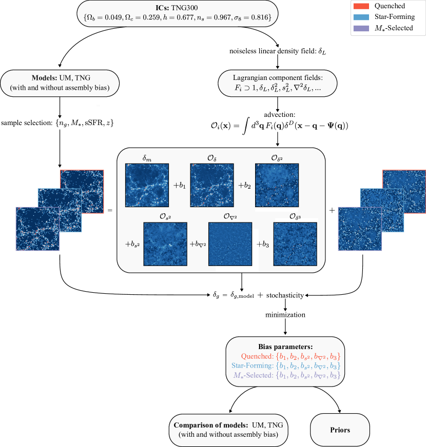
Figure 1: Visualization of the methodology of this work: starting from the same initial conditions (TNG300), we obtain both the galaxy density field $\delta_{g}$ for each model (UM and TNG, with and without assembly bias) and the noiseless linear density field $\delta_{L}$. Using the latter, we construct the bias-weighted fields $\mathcal{O}_{i}$ at redshift $z$ via advection. These constitute a deterministic model $\delta_{g,\mathrm{model}}$ that differs from the galaxy density field $\delta_{g}$ only by a stochastic term $\epsilon$ (see Equation 6), which we minimize to solve for the best-fit bias parameters of each sample. Finally, we compare results between the models and set priors for use in cosmological inferences. In this figure, we visualize the density field $\delta_{g}$ and stochasticity $\epsilon$ at $z=0.5$ for a high number density sample in TNG.

In the remainder of this text, we assume that all of our bias parameter measurements result from this estimator $\hat{b}_{i}$. To improve readability, we henceforth refer to the estimator for bias parameters as simply $b_{i}$. Our methodology for obtaining this estimate, as well as our subsequent analysis, is summarized in Figure 1.

3 Simulations

Using the techniques outlined in §2, we can now compare different models of galaxy formation. The models and samples we examine are detailed in §3.1 and §3.2 below.

3.1 Models of galaxy formation

We use two primary galaxy formation models in this study: UniverseMachine (UM), an empirical semi-analytic model, and IllustrisTNG (TNG), a hydrodynamical model. To compare UM and TNG, we create matched galaxy samples from each model, as explained in §3.2. We also create matched samples from an additional model of the galaxy–halo connection: a mass-dependent, non-parametric HOD that removes galaxy assembly bias from both UM and TNG, as detailed in §5.1. From these sample catalogs, we obtain the galaxy overdensity field $\delta_{g}(\mathbf{k})$, which we use to solve for the best-fit bias parameter estimator $\hat{b}_{i}(k)$, as written in Equations 12-14. To make a direct comparison between the bias parameters measured from the two models, we set identical initial conditions by running the UniverseMachine DR1 model on the non-baryonic physics “dark matter only” counterpart to TNG300, known as TNG300-1 Dark, with the following cosmological parameters: {$\Omega_{b}=0.0486,\Omega_{c}=0.2589,h=0.6774,n_{s}=0.9667,\sigma_{8}=0.8159$}. This ensures that the large-scale structure is identical in the UM and TNG boxes.

The UniverseMachine (UM) is an empirical model of galaxy formation that links star formation to properties of the host halo (Behroozi et al., 2019). Specifically, UM models galaxy formation and evolution by constraining the star formation rate (SFR) of a galaxy as a function of the dark matter halo’s maximum circular velocity, redshift, and accretion history. UM thus assigns an SFR distribution to each galaxy from this parameter space and integrates the SFR along the merger tree of each galaxy’s host halo. From this, UM obtains a stellar mass and UV luminosity and compares the statistics of these observables to that of the real universe to obtain a likelihood of the original guess. This likelihood is fed to a Markov Chain Monte Carlo algorithm, which returns the posterior distribution of the model parameters and the best-fitting parameters in the 44-dimensional parameter space.

The IllustrisTNG project (TNG) is a full magnetohydrodynamic cosmological simulation that includes prescriptions for gas cooling, star formation, stellar feedback, and supermassive black hole growth and feedback. TNG uses the moving-mesh hydrodynamic and gravity N-body code arepo (Springel, 2010) to model galaxy evolution and obtains initial conditions at $z=127$ using the N-GenIC code (Springel et al., 2005). Dark matter halos are identified as groups using the friends-of-friends (FoF) algorithm (Davis et al., 1985). Galaxies are consequently defined as subhaloes within each FoF group via the subfind algorithm (Springel et al., 2001; Dolag et al., 2009). We consider the largest run in their simulation suite, TNG300, part of their publicly available data release (Nelson et al., 2021). This box has a size of $L_{\mathrm{box}}=205\,h^{-1}{\rm Mpc}$, which is $\sim 300$ Mpc, with 2500³ dark matter and gas particles each.

3.2 Selecting galaxies at a target number density

We create matched samples of galaxies from each galaxy formation model (UM and TNG) to mimic the target number density and redshift spanned by DESI’s selection of Luminous Red Galaxies (LRGs) and Emission Line Galaxies (ELGs) (DESI Collaboration et al., 2016). LRGs are early-type, elliptical galaxies with red rest-frame optical wavelengths that occupy the redshift range $z\approx[0.4,1.0]$. ELGs are late-type, spiral galaxies with blue rest-frame optical wavelengths that occupy the redshift range $z\approx[0.6,1.6]$. Each sample has a target number density of $\bar{n}_{g}\approx 5\times 10^{-4}$ $[\,h^{-1}{\rm Mpc}]^{-3}$ in DESI (Zhou et al., 2023; Yuan et al., 2022).

To encompass a significant range of redshifts for the LRG and ELG target galaxies, our data comprises snapshots at redshifts $z=\{0.0,0.5,1.0,1.5\}$. At each of these snapshots, we make number density cuts based on stellar mass ($M_{*}$) and specific star formation rate (sSFR). These $M_{*}$ and sSFR cuts act as a proxy for galaxy color so that we can select samples similar to DESI’s LRGs and ELGs in our study. We thereby create populations that mimic quenched galaxies, with little-to-no active star formation, as well as galaxies with currently ongoing star formation (Martig et al., 2009), in rough correspondence to the LRGs and ELGs that DESI targets, respectively. For completeness, we also use the $M_{*}$ cuts to create a general $M_{*}$-selected population; this combined sample of the quenched and star-forming galaxies is treated as an additional galaxy type in our study.

To account for variation in the number density achieved by future surveys, we choose three target number densities for each galaxy formation model at all redshifts. These include a “low” number density ($10^{-3}$ $[\,h^{-1}{\rm Mpc}]^{-3}$), corresponding to a realistic, conservative cut that matches the sum of DESI’s target number densities for ELGs and LRGs, as well as a medium (3.9$\times 10^{-3}$ $[\,h^{-1}{\rm Mpc}]^{-3}$) and high number density cut (6.8$\times 10^{-3}$ $[\,h^{-1}{\rm Mpc}]^{-3}$), which are increasingly more ambitious to achieve in very wide-area galaxy redshift surveys. Overall, we investigate 144 galaxy samples: three selections in number density; quenched, star-forming, and $M_{*}$-selected galaxies; UM and TNG, as well as assembly-bias-removed versions of each; and four redshift bins. The number densities of each sample, as well as the thresholds in $M_{*}$ and sSFR that define each galaxy type, are detailed in Table 3 of the Appendix. A visual illustration of our selection process, as well as the distribution of sSFR and $M_{*}$ in the TNG and UM galaxy formation models, is shown in Fig. 2.

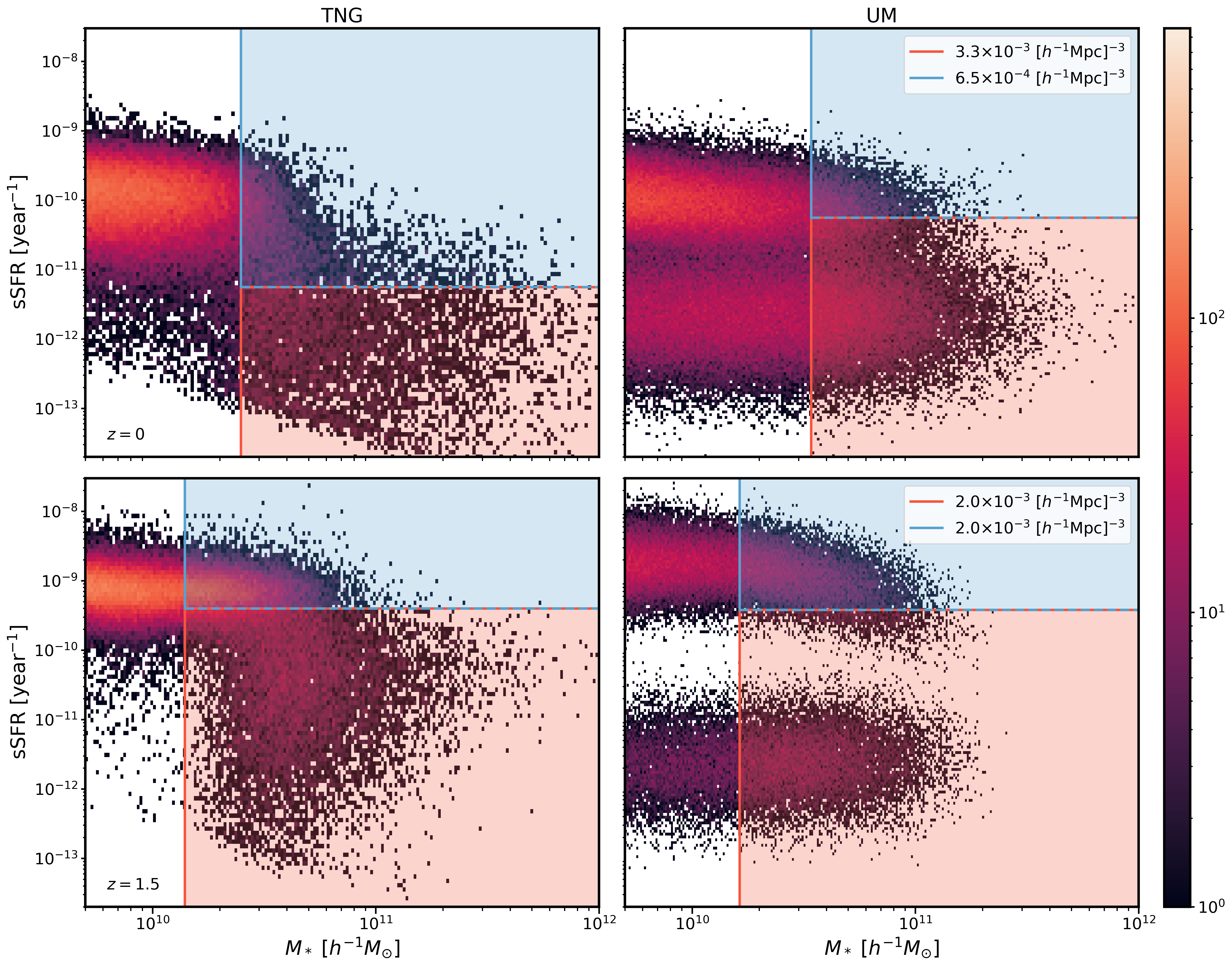
Figure 2: A 2D histogram of $M_{*}$ and sSFR for TNG and UM galaxies at redshifts $z=0$ (top panel) and $z=1.5$ (bottom panel). The red and blue shaded regions mark the $M_{*}$ and sSFR cuts which separate the quenched and star-forming samples, respectively. The number density for each population is shown in the legend (medium number density, medium $M_{*}$).

To create these samples, we first reach our target number density by making a cut in stellar mass. As listed in the “$M_{*}$-selected” column of Table 3, these target number densities include a low, medium, and high-density cut, which entails a high, medium, and low stellar mass cut respectively. Then, to distinguish between star-forming and quenched galaxies at redshifts $z=\{0.5,1.0,1.5\}$, we divide the $M_{*}$-selected sample of galaxies in half by making a cut in sSFR, as depicted by the horizontal dashed blue and red lines in Figure 2. This ensures that each population has identical number densities. We calculate the sSFR using each galaxy simulation’s instantaneous star formation rate (SFR) and stellar mass.

The samples at redshift $z=0$ follow a slightly modified procedure, as there are not enough star-forming galaxies in TNG to evenly split the samples at this redshift. We instead divide the $M_{*}$-selected sample of galaxies so that there are five times as many quenched galaxies as star-forming galaxies ($n_{g\mathrm{,quenched}}=5n_{g\mathrm{,star-forming}})$, such that the number density of star-forming galaxies are closer to our density selections at other redshifts. This is reflected in the target number densities listed for each sample in the “Quenched” and “Star-Forming” columns of Table 3. It is important to note that while we achieved an even split of quenched and star-forming galaxies in UM, we chose to repeat this modified procedure for both simulations. This is so that we could maintain identical conditions for both models and ultimately enable a direct comparison of our bias measurements.

Figure 2 depicts our selection of quenched and star-forming galaxy samples in the $M_{*}$-sSFR parameter space of UM and TNG with red and blue shaded regions. To show how the galaxy catalog evolves with redshift in both simulations, the first row shows our selections at $z=0$, and the second row shows our selections at $z=1.5$. As the red-shaded region in the upper left panel visualizes, the sSFR cut for quenched galaxies in TNG at $z=0$ is not unreasonably high, showing that this modified selection procedure is a suitable one. Similarly, the upper right panel makes it clear that there are more quenched galaxies than star-forming galaxies in UM at $z=0$ due to this modified selection procedure, as indicated by the higher sSFR cut.

We note that there are many galaxies with zero SFR in TNG, particularly at redshift $z=0$. This likely contributes to the overabundance of quenched galaxies that we find in TNG at $z=0$, as roughly $67-70\%$ of the galaxies in our selection at this snapshot are assigned a SFR of zero, compared to $\sim 6\%$ at $z=1.5$, and $<0.5\%$ of the UM galaxy samples across all redshifts and number density cuts. To avoid numerical errors from taking the log of zero SFR, we offset the SFR of each galaxy by a trace amount ($10^{-13}\,M_{\odot}(h{\rm yr})^{-1}$). As a result, these zero-SFR galaxies are not visible in Figure 2, but are included in the quenched galaxy sample. For consistency, we implement this offset for all samples at redshifts $z=\{0.0,0.5,1.0,1.5\}$ in both TNG and UM.

4 Results

Having created the galaxy samples at each redshift and target number density for both the TNG and UM galaxy formation models, we now find the best-fit bias parameters using the procedure described in §2.2. The key measurements are presented in §4.1 in the form of the $b_{2}(b_{1})$, $b_{s^{2}}(b_{1})$, $b_{\nabla^{2}}(b_{1})$, and $b_{3}(b_{1})$ bias relations. In §4.2, we make a 1:1 comparison of these measured bias parameters across the galaxy formation models.

4.1 The bias relations

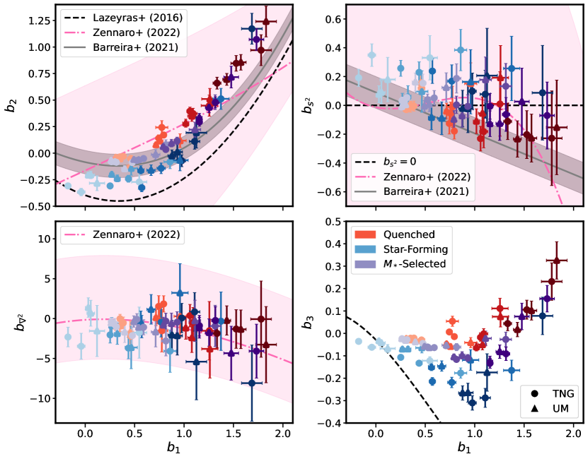
Figure 3: The bias parameter relations as a function of $b_{1}$ at $z=\{0.0,0.5,1.0,1.5\}$ for each sample of galaxies in UM (triangles) and TNG (circles), including quenched (red), star-forming (blue), and the $M_{*}$-selected population (purple). The color intensity (light to dark) maps to the redshift (low to high). The error bars are calculated according to the steps outlined in Appendix C of Kokron et al. (2022). Best-fit relations for halos (Lazeyras et al., 2016) and galaxies (Barreira et al., 2021; Zennaro et al., 2022) from past works are shown as comparison.

To compare our measurements to those in the literature, we examine the $b_{2}(b_{1})$, $b_{s^{2}}(b_{1})$, $b_{\nabla^{2}}(b_{1})$, and $b_{3}(b_{1})$ bias relations. Using the best-fit bias parameter solution in Equation 12, we can obtain measurements of the bias parameters for each galaxy sample at a chosen $k_{\mathrm{max}}$. We use $k_{\mathrm{max}}=0.2\ h{\rm Mpc}^{-1}$ as conservative estimate to report our final results, as it has been shown that perturbative approaches like our own are successful in describing the clustering of galaxies down to these scales (Baldauf et al., 2016). In Appendix B we check that we recover the expectation of $b_{1}$ from the cross-spectrum definition of the linear bias. We additionally show, in Appendix B, that until $k_{\rm max}=0.2\ h{\rm Mpc}^{-1}$, we do not find a strong running with scale for our measured parameters. Once we calculate the bias parameters at $k_{\mathrm{max}}=0.2\ h{\rm Mpc}^{-1}$ for each of our galaxy samples, we plot the higher-order bias parameters as a function of the linear bias parameter $b_{1}$. We refer to these as the bias relations.

These measurements are presented in Figure 3 for UM and TNG as triangles and circles, respectively. In each panel, we plot the measured bias relations $b_{2}(b_{1})$, $b_{s^{2}}(b_{1})$, $b_{\nabla^{2}}(b_{1})$, and $b_{3}(b_{1})$ for quenched (red), star-forming (blue), and the $M_{*}$-selected galaxy population (purple). Each data point represents a sample of galaxies selected from redshifts $z=\{0.0,0.5,1.0,1.5\}$ using the target number density cut method described in §3.2. The color intensity maps to the redshift of the sample: lighter shades represent low redshift, and darker shades represent high redshift. For each higher-order bias parameter, we also plot as a dashed line some relevant best-fit measurements from the literature (Lazeyras et al., 2016; Barreira et al., 2021; Zennaro et al., 2022), which we explain in more detail in the subsequent sections for each parameter.

There are several interesting trends in this result. In each panel of Figure 3, we see that the central values of the linear bias $b_{1}$ parameter measurements on the $x-$axis range from $b_{1}\approx[-0.2,1.9]$. The lower end of that range, from $b_{1}\approx[-0.2,0.5]$, is primarily occupied by low-redshift, star-forming galaxies (light, blue points), while the higher end of that range, from $b_{1}\approx[1.5,1.9]$, is dominated by high-redshift, quenched galaxies (dark, red points). This is partly because quenched galaxies are hosted in more massive (Woo et al., 2013), and therefore, more strongly clustered halos than their star-forming counterparts. As a result, they have a higher linear bias $b_{1}$ measurement (Bose et al., 2023). Meanwhile, the trend in redshift is due to the fact that the linear bias $b_{1}$ parameter correlates positively not only with halo mass, but also redshift $z$ (Cole & Kaiser, 1989; Mo & White, 1996); the same mass halo is a much rarer object at high redshift than today. As all samples are created with roughly similar cuts in stellar mass (see Table 3 in the Appendix), it is therefore consistent with literature that the higher $b_{1}$ measurements in Figure 3 are dominated by high redshift galaxies. We return to these measurements and a comparison to theoretical expectations in §5.2, and now focus on the bias relations for the individual parameters shown in Fig. 3.

4.1.1 $b_{2}(b_{1})$

Having confirmed that our results in Figure 3 agree with basic intuition about the behavior of galaxy bias, we examine each bias relation in detail, starting with $b_{2}(b_{1})$ (top left). The central values of the $b_{2}$ measurements range from $b_{2}\approx[-0.4,1.3]$. Star-forming galaxies mostly occupy the lower end of that range, from $b_{2}\approx[-0.4,0.2]$, although two higher redshift TNG star-forming samples with $b_{1}>1.3$ reach $b_{2}\sim 0.5$ and $\sim 1.1$. In contrast, quenched galaxies occupy a much broader range of parameter space, from $b_{2}\approx[-0.2,1.3]$. The broadly observed trend is that given a value of $b_{1}$, quenched galaxies have a higher $b_{2}$ than star-forming galaxies. In other words, even if quenched and star-forming galaxies have an identical first-order response to changes in large-scale matter overdensities, the former has a larger second-order response. This can be understood as a difference in the shape of the halo occupation distribution for the two galaxy types, which we return to in 5.2.

As we do for the other bias parameters in the following sections, we compare our $b_{2}(b_{1})$ results to several similar measurements in the literature. We convert any Eulerian bias parameter measurements into the appropriate Lagrangian equivalent using the co-evolution relations between Eulerian and Lagrangian bias (Lazeyras et al., 2016; Abidi & Baldauf, 2018). We also separate our discussion into analyses of halos and analyses on galaxies. For the former, we plot Lazeyras et al. (2016)’s cubic polynomial fit of the $b_{2}(b_{1})$ bias relation for dark matter halos, which are split by mass (black dashed line). This measurement employs separate universe simulations to measure Eulerian local-in-matter (LIMD) bias parameters. Although dark matter halos also trace dark matter, their bias is closely related to, but not equivalent to, that of galaxies. As we show later in Equation 17, galaxy bias is an integral of halo bias, the halo mass function, and the halo occupation distribution. Given that we measure the bias relations for galaxies and not dark matter halos in this study, it is consistent with theoretical predictions that our values are different compared to Lazeyras et al. (2016); this is also what Zennaro et al. (2022) find in measuring the second-order Lagrangian bias $b_{2}$ for galaxies. This is analytically understood from Equation 17, as the HOD upweights higher mass haloes compared to the halo $b_{1}$ that matches the galaxy $b_{1}$. The relation between galaxy and halo bias is further explored in §5.2.

The other two best-fit relations come from galaxies and are more directly comparable to our measurements. First is a best-fit relation in which Zennaro et al. (2022) measure the Lagrangian bias relations (pink dashed-dotted line) for galaxies selected using the SubHalo Abundance Matching extended algorithm (SHAMe). The authors set priors using a hypervolume that encloses all of their galaxy samples (pink-shaded region). These priors are noticeably larger than our measurements. This is not surprising; the SHAMe parameters picked in Zennaro et al. (2022) correspond to galaxy–halo connections that are much broader than what is consistent with known data on galaxy–halo connections. Thus, our tighter constraints are not necessarily a reflection of the model performance but of the realistic types of galaxies we have selected, i.e., quenched and star-forming populations that mimic DESI LRG and ELG targets.

The second galaxy bias measurement shown in Figure 3 is a best-fit relation for Eulerian bias parameters determined using field-level forward models of galaxy clustering (grey solid line). With this method, Barreira et al. (2021) fit a cubic polynomial to the measured bias relation of TNG galaxies (grey solid line). To create a Gaussian prior, this fit is assigned a $b_{1}$-independent $1\sigma$ standard deviation (grey shaded region). Our measurements agree with the general shape of these $b_{2}(b_{1})$ fits but do not exactly match either of them. For instance, in comparison to both of these fits, our measurements of $b_{2}$ are lower at lower $b_{1}$, and higher at higher $b_{1}$.

4.1.2 $b_{s^{2}}(b_{1})$

In the top right panel of Figure 3, we plot our measurements of the $b_{s^{2}}(b_{1})$ bias relation, which ranges in its central value from $b_{s^{2}}\approx[-0.3,0.4]$. We show in comparison the Lagrangian local-in-matter (LLIMD) prediction, which assumes $b_{s^{2}}=0$ (black dashed line). The LLIMD ansatz assumes that the impact of the tidal field on the Lagrangian-space initial positions is negligible (Lazeyras et al., 2016; Lazeyras & Schmidt, 2018). This is an approximation which, while qualitatively accurate, does not strictly hold. Multiple measurements in the literature have found signatures of a nonzero halo tidal bias parameter, and overwhelmingly find that $b^{L}_{s^{2}}<0$ for mass-selected halos (Saito et al., 2014; Modi et al., 2017; Lazeyras & Schmidt, 2018). We include in Figure 3 two measurements from the literature that contradict the LLIMD prediction in galaxies. The first is the best-fit measurement of Lagrangian bias for SHAMe galaxies from Zennaro et al. (2022) (pink dashed line and shaded region), and the second is the best-fit measurement of Eulerian bias parameters for TNG galaxies from Barreira et al. (2021) (grey solid line and shaded region). In Figure 3 we see clear broad trends: the star-forming sample exhibits mildly positive $b_{s^{2}}$ with no strong scaling with the underlying $b_{1}$, while the quenched galaxies have negative tidal bias that increases in amplitude with $b_{1}$. It is perhaps surprising that the galaxy types appear to be split by the LLIMD approximation $b_{s^{2}}=0$, as the positive tidal bias in star-forming galaxies is in contrast to the aforementioned negatively biased measurements of $b_{s^{2}}$ from halos in the literature. It has been noted previously that spin-dependent assembly bias could push $b_{s^{2}}$ to positive values in halos (Lazeyras et al., 2021). In this case, a positive $b_{s^{2}}$ in star-forming galaxies could be a clear signal of assembly bias in their formation. However, we discuss in §5.1, and show in Figure 4 that removing assembly bias in the star-forming galaxy samples has a mild impact on $b_{s^{2}}$. We comment more broadly on the potential impact of assembly bias on our other parameters in §5.1.

4.1.3 $b_{\nabla^{2}}(b_{1})$

We plot the bias relation for $b_{\nabla^{2}}(b_{1})$ in the bottom left panel. The $\nabla^{2}\delta$ field is a counter-term in the pure EFT bias expansion of halos. Still, physical intuition can be gleaned from considering that the Laplacian of the Lagrangian density field around peaks corresponds to their curvature. That is, highly concentrated peaks are associated with regions with large $\nabla^{2}\delta_{L}$. Then, the $b_{\nabla^{2}}$ parameter tells us how haloes form not just in matter overdensities, but also in overdensities of varying sharpness given a similarly sized overdensity. In the case of dark dark matter halos, the associated bias $b_{\nabla^{2}}$ is expected to be on the order of the squared Lagrangian radius $R_{L}$ of halos such that $|b_{\nabla^{2}}(b_{1})|\sim R_{L}^{2}$(Lazeyras & Schmidt, 2018, 2019; Zennaro et al., 2022). Hydrodynamical effects that re-distribute the distribution of matter on one-halo scales are therefore also expected to affect the inferred value of $b_{\nabla^{2}}$. It ranges in its central value from $b_{\nabla^{2}}\approx[-9,4]$, and is by far the least constrained of the five bias parameters. The $b_{\nabla^{2}}$ bias parameter consequently has the largest error bars, as the $\mathcal{O}_{\nabla^{2}}$ field only has appreciable contributions at scales comparable to our filtering scale of $k_{\mathrm{max}}=0.2\ h{\rm Mpc}^{-1}$. The error bars thus drop dramatically as a function of $k_{\mathrm{max}}$, as Figure 11 shows.

For comparison, we include the best-fit measurement of Lagrangian bias parameters for SHAMe galaxies by Zennaro et al. (2022) (pink dashed line). Their priors are enclosed in the pink-shaded region. We find that our measurements for $b_{\nabla^{2}}$ do not show a dependence on the galaxy population type (quenched, star-forming, $M_{*}$-selected). This contrasts with the other four bias parameters, which give distinct measurements depending on the type of galaxy distribution. There are many reasons why this could be the case. The $\mathcal{O}_{\nabla^{2}}$ operator is sensitive to the curvature of the field around its peaks but is also related to small-scale one-halo effects that affect the inner distribution of matter in a halo. Baryonic feedback, tidal stripping, assembly bias (the effect of which is explored in §5.1), and even halo-finding effects could presumably influence $b_{\nabla^{2}}$ for a population of halos with similar values of other biases. Indeed, the $b_{\nabla^{2}}$ parameter is a counter-term that absorbs the sensitivity of the bias expansion to these degenerate small-scale physics.

4.1.4 $b_{3}(b_{1})$

In the bottom right panel, we plot the final bias relation for $b_{3}(b_{1})$, which measures the response of the tracer number density to third-order changes in the dark matter density field. Our measurements of the cubic bias parameter range from $b_{3}\approx[-0.4,0.4]$ in central value, with quenched galaxies occupying the higher end of that range (biased) and star-forming galaxies the lower end (anti-biased). The galaxy populations are thus split by $b_{3}=0$, like the $b_{s^{2}}$ measurements. This has the effect that quenched galaxies are more positively biased than star-forming galaxies at a given $b_{1}$, similar to the $b_{2}(b_{1})$ relation.

We include one comparison to literature in the figure, given by the fitting function from Lazeyras et al. (2016) (black dashed line). This fit remains negative even though our measurements become more positive for higher $b_{1}$ values. These larger values are especially true for the quenched galaxies, while the star-forming samples better follow the $b_{3}(b_{1})$ fit: they remain anti-biased, aside from one outlier in TNG at high $b_{1}$.

However, it should be noted that we are measuring some “effective” cubic bias parameter rather than the actual $b_{3}$. This is because our measurement of $b_{3}$ includes any error or deviations due to missing higher-order operators, as our model includes only a finite number of bias parameters. Although the effects should be slight, these residual differences could contribute to the consistently larger bias parameter values that we measure. The $b_{3}$ relation from Lazeyras et al. (2016) also only applies to dark matter halos, and differences between galaxy and halo bias arising from the HOD are exacerbated for a bias parameter that scales more aggressively with halo mass, as is the case for the halo $b_{3}$ compared to $b_{1}$ or $b_{2}$.

Overall, for each bias relation, we see that our measurements largely follow the trend lines established by previous best-fit measurements in the literature. We also find that quenched and star-forming galaxies occupy different parts of parameter space for each of the bias relations, aside from $b_{\nabla}^{2}(b_{1})$. The bias for the $M_{*}$-selected population falls in between the other two measurements at a given number density cut, redshift, and galaxy formation model. Using the terminology presented in §5.1, this is explained by recognizing that the $M_{*}$-selected HOD is a linear combination of the quenched and star-forming samples.

4.2 Impact of galaxy formation model

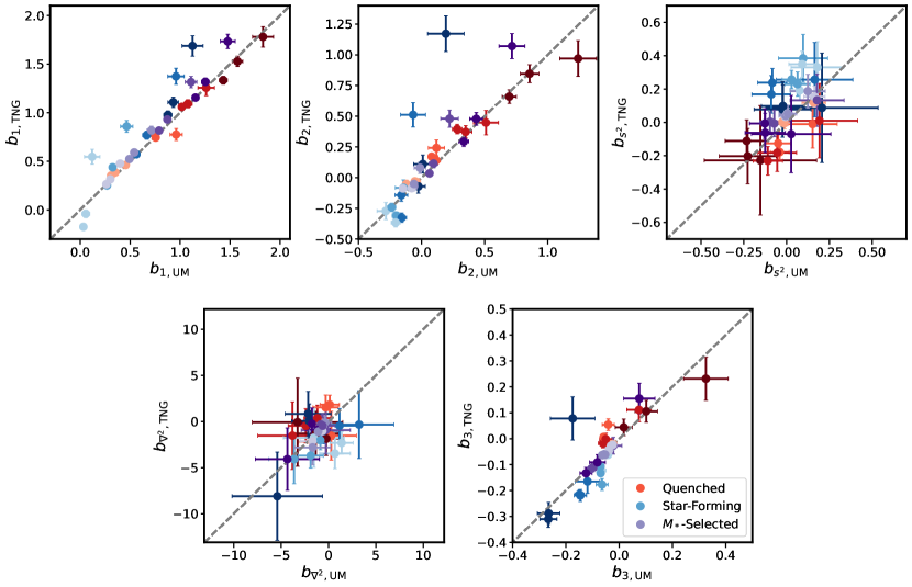
Figure 4: The bias parameter measurements of TNG galaxies in comparison to UM galaxies for quenched (red), star-forming (blue), and $M_{*}$-selected samples. The color intensity (light to dark) maps to the redshift (low to high). A 1:1 dashed line is plotted for reference.

We further investigate how the measurements vary as a function of galaxy formation model by comparing each measurement between UM and TNG directly, shown in Figure 4. Here, we plot the bias parameters measured in TNG against those measured in UM at the same redshift ($z=\{0.0,0.5,1.0,1.5\}$), number density (low, medium, high), and galaxy selection type (quenched, star-forming, $M_{*}$-selected). Looking at the samples collectively, we find that TNG and UM generally measure comparable values for each bias parameter, as there is no significant deviation from the 1:1 line. However, we find larger scatter in $b_{s^{2}}$ and $b_{\nabla^{2}}$ as they are less well-measured than the $b_{1}$, $b_{2}$, and $b_{3}$ parameters.

Interestingly, the populations that deviate from the 1:1 relations in $b_{1}$, $b_{2}$, and $b_{3}$ belong to the lowest number density samples. This suggests that TNG and UM agree reasonably well further down the stellar mass function but disagree on the bias behavior of the most massive galaxies. This could be for several reasons: for example, the high-mass end of the halo mass function may be easily affected by different galaxy formation prescriptions, as it is less constrained by current data, more sensitive to uncertain feedback; the discrepancies for rare samples may also be impacted by the limited box size of TNG. These outliers are also primarily star-forming galaxies, especially in the linear bias $b_{1}$, suggesting that there is wider scatter in that population than in the quenched sample. This increase in the linear bias of star-forming galaxies in TNG compared to UM can also be seen in Figures 11 and 10 in Appendix B.

Despite this broader agreement when considering the samples as a whole, we notice a difference between the models when considering the behavior of the quenched and star-forming samples separately, specifically in the case of the tidal bias $b_{s^{2}}$. As discussed in §4.1.2, we find that the quenched galaxies are generally more negatively biased in $b_{s^{2}}$ than the star-forming galaxies, which tend to be positively biased; however, Figure 4 shows that these positively biased star-forming galaxies have comparatively higher bias in TNG than their counterparts in UM. The converse is true of the quenched galaxies, which have lower bias in TNG compared to UM, albeit to a lesser extent. Combining these two effects means that the aforementioned differences between the tidal bias $b_{s^{2}}$ of quenched and star-forming galaxies hold for each model but are more pronounced in TNG than in UM. These trends are more readily apparent in Figure 12 of Appendix C, which directly compares the bias parameters between the galaxy types for each model. However, while it may be worth further examining this disagreement in a larger box that can better constrain $b_{s}^{2}$, the tidal bias likely does not have a large enough impact on the power spectrum for these differences to be detected observationally unless higher-order information such as the bispectrum is included.

5 Discussion

In this section, we analyze the results presented in §4. We first discuss the impact of assembly bias in §5.1 and follow this up by comparing our bias parameter measurements to theoretically motivated predictions in §5.2. Finally, we examine the degree of non-Poisson stochasticity in our samples in §5.3, and end the discussion by setting priors on the bias parameters in §5.4.

5.1 Assembly bias signature

Halo assembly bias refers to the dependence of halo clustering on secondary halo properties, such as assembly history, in addition to the primary property of halo mass (Gao et al., 2005; Wechsler et al., 2006; Dalal et al., 2008; Mansfield & Kravtsov, 2020). We are interested in the impact of halo assembly bias on galaxy clustering (Zhu et al., 2006; Croton et al., 2007) and in particular, its effects on our measurements of the galaxy bias parameters. We refer to this phenomenon interchangeably as both galaxy assembly bias and assembly bias.

Unlike simple parameterizations such as HOD models, which explicitly populate halos with galaxies only as a function of halo mass (Scoccimarro et al., 2001; Berlind & Weinberg, 2002), hydrodynamical simulations like TNG and empirical models like UM that are based on full halo formation histories automatically encode galaxy assembly bias into their modeling approach (Artale et al., 2018; Bose et al., 2019; Hadzhiyska et al., 2021b; Yuan et al., 2022). However, the true extent of galaxy assembly bias present in specific galaxy samples is unknown (Wang et al., 2013; Hearin et al., 2016; Zentner et al., 2019).

For our study to properly inform future clustering analyses on the full range of uncertainty in galaxy formation physics, it is thus crucial that we consider models both with and without assembly bias (Zentner et al., 2014). This is especially important when considering separate galaxy population types, such as the quenched and star-forming populations that we examine in this study, since such samples are expected to be impacted by assembly bias to different degrees (Croton et al., 2007; Hadzhiyska et al., 2021c; Yuan et al., 2022). We now present our method of removing assembly bias from each of our samples, as well as its subsequent impact on their bias parameter measurements.

To remove assembly bias, we follow the standard HOD assumption that the occupation of halos by central $\left\langle N_{\mathrm{cen}}\right\rangle$ and satellite galaxies $\left\langle N_{\mathrm{sat}}\right\rangle$ are two independent processes:

$$\langle N(M)\rangle=\left\langle N_{\mathrm{cen}}\right\rangle+\left\langle N_{\mathrm{sat}}\right\rangle,$$ (16)

where $\langle N(M)\rangle$ is the HOD, or mean number of galaxies at a halo mass $M$, $\left\langle N_{\mathrm{cen}}\right\rangle$ is the mean number of central galaxies and $\left\langle N_{\mathrm{sat}}\right\rangle$ represents the mean number of satellite galaxies. We base our subsequent technique on a standard shuffling method in which the galaxy occupation within each halo is randomly exchanged with that of another halo in the same mass bin (Croton et al., 2007; Contreras et al., 2019; Xu et al., 2021). We follow a slightly modified procedure, following the example of Yuan et al. (2022):

1. Bin the dark matter halos by their mass from 1$\times 10^{10}$ to 1$\times 10^{15}$ M$\sun$/h. Measure the central and satellite galaxy occupation $\left\langle N_{\mathrm{cen}}\right\rangle$ and $\left\langle N_{\mathrm{sat}}\right\rangle$ in each mass bin.

2. Given the mass bin of each halo, perform a Bernoulli draw using $\left\langle N_{\mathrm{cen}}\right\rangle$ to determine whether it is populated with a central galaxy. If so, assign that central galaxy the same position as its host halo.

3. For each satellite galaxy, calculate the offset of its position from the position of its host halo. Construct a catalog of satellite offsets binned by halo mass.

4. Iterate through each central halo, and perform a Poisson draw using $\left\langle N_{\mathrm{sat}}\right\rangle$ to determine the number of satellite galaxies it hosts. Assign positions to those satellite galaxies by randomly selecting offsets from halos in the same mass bin.

As with the standard shuffling method, this technique eliminates any dependence of the HOD on any other property besides halo mass. Using the definition of galaxy assembly bias set forth by Wechsler & Tinker (2018), this removes assembly bias from our samples, while by construction preserving the HOD $\langle N(M)\rangle$ of each galaxy sample, as well as $\left\langle N_{\mathrm{cen}}\right\rangle$ and $\left\langle N_{\mathrm{sat}}\right\rangle$. Still, there are two key differences between our procedure and the standard shuffling technique.

First, we populate the halos by randomly drawing from a probability distribution rather than swapping existing galaxies between halos. Because each dark matter halo has either one or zero central galaxies, we assign central galaxies to halos using the Bernoulli distribution and model the satellite occupation using the Poisson distribution (Zheng et al., 2005). However, this means that the number density of galaxies $n_{g}$ in the shuffled samples is not exactly preserved, as there is a very small scatter around $n_{g}$ due to the Poisson and Bernoulli variance.

Second, by populating central and satellite galaxies separately, rather than moving satellites alongside their centrals, we ensure that we also wipe out galactic conformity. This is a phenomenon in which the characteristics of the central galaxy influence the characteristics of its surrounding satellites, e.g., quenched centrals are more likely to be surrounded by quenched satellites (Weinmann et al., 2006; Kauffmann et al., 2013; Kawinwanichakij et al., 2016). It is important to shuffle the centrals and galaxies separately so that this correlation is eliminated, and the only factor influencing $\left\langle N_{\mathrm{cen}}\right\rangle$ and $\left\langle N_{\mathrm{sat}}\right\rangle$ is the halo mass $M$.

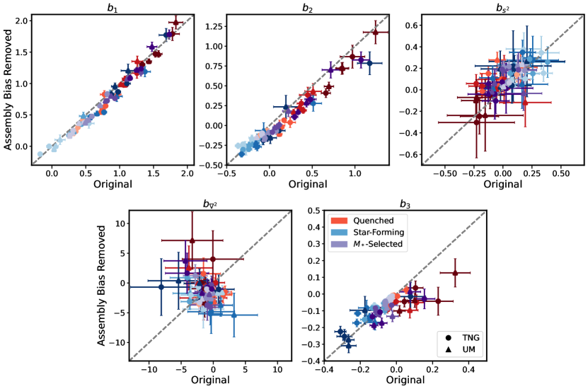
Figure 5: The effect of AB removal on each of the bias parameter measurements. The new measurements without AB are plotted against the original measurements with AB at $z=\{0.0,0.5,1.0,1.5\}$ for each sample of galaxies in UM (triangles) and TNG (circles), including quenched (red), star-forming (blue), and the $M_{*}$-selected population (purple). The color intensity (light to dark) maps to the redshift (low to high). A 1:1 dashed line is plotted for reference.

We perform this shuffling-based procedure on each of the 72 galaxy samples we created in §3.2, and obtain an AB-removed version of each distribution of galaxies in UM and TNG. We measure the bias parameters for these AB-removed samples using the methodology of §2.2, and present our results in Figure 5. Here, we have plotted the bias parameter measurements for each of the AB-removed samples against the measurements from our original samples with assembly bias. The quenched galaxies are plotted in red, the star-forming in blue, and the $M_{*}$-selected galaxies in purple.

For powers of the matter density field, i.e., the LIMD parameters $b_{1}$, $b_{2}$, and $b_{3}$, removing assembly bias consistently reduces the bias parameter measurements. This is consistent with findings by Hadzhiyska et al. (2023) that both ELGs and LRGs exhibit signatures of assembly bias in which the AB-removed samples are less clustered than the original samples. We find that this effect is stronger for higher-order powers and for higher redshift samples.

In contrast, there is no discernible trend with the non-local tidal bias parameter $b_{s^{2}}$, while the $b_{\nabla^{2}}$ term interestingly shows an inversion of its original values: negative measurements become positive with AB removal, and positive measurements become negative. This effect slightly differs between galaxy populations, such that quenched galaxies become more positive than star-forming galaxies post AB-removal. As a result, quenched and star-forming occupy more distinct parts of AB-removed bias parameter space. This is in contrast to the original $b_{\nabla^{2}}$ measurements, where there is no apparent pattern, as noted in §4.1.3.

As defined in Wechsler & Tinker (2018), galaxy assembly bias is caused by halo assembly bias in addition to a dependence of the number of galaxies within dark matter halos on a secondary halo property besides halo mass. Since we remove any secondary dependence of the halo occupation distribution through our assembly bias-removal procedure, any changes that we see in the original bias parameter measurements compared to the AB-removed bias parameter measurements would mean that we have indeed detected a signature of assembly bias. We thus see evidence for assembly bias in all bias parameters included in our bias expansion model, except for $b_{s^{2}}$.

However, interpreting the exact root of these changes is not straightforward, as under the halo model (Seljak, 2000), galaxy bias can be estimated using what is known as analytic or effective bias (Baugh et al., 1999; Benson et al., 2000). Through this parameterization, the galaxy bias parameters $b_{i}$ become a function of the mean galaxy number density $\bar{n}_{g}$, halo mass function (HMF) $\frac{dn}{dM}$, the HOD $\langle N(M)\rangle$, and the halo bias $b_{i,h}(M)$:

$$b_{i}=\frac{1}{\bar{n}_{g}}\int dM\frac{dn}{dM}b_{i,h}(M)\langle N(M)\rangle.$$ (17)

The mean number density of galaxies $\bar{n}_{g}$ is similarly a function of the HMF $\frac{dn}{dM}$ and the HOD $\langle N(M)\rangle$:

$$\bar{n}_{g}=\int dM\frac{dn}{dM}\langle N(M)\rangle.$$ (18)

Understanding how the galaxy bias parameters $b_{i,g}$ change with AB removal would therefore require understanding how exactly the mean galaxy number density $\bar{n}_{g}$, halo mass function (HMF) $\frac{dn}{dM}$, the HOD $\langle N(M)\rangle$, and the halo bias $b_{i,h}(M)$ are each impacted by an additional dependence on a secondary halo property. For example, there is a known dependence of the HMF on environment, with the most massive halos forming only in the densest environments (Crain et al., 2009). However, the relationship of the HOD and halo bias with assembly bias has proven to be quite complicated. For instance, Hadzhiyska et al. (2020) find that galaxy clustering from the basic HOD, which is dependent only on halo mass $M$, underpredicts the TNG300-1 galaxy correlation function by $\sim$15%. Furthermore, the degree to which AB impacts galaxy clustering seems to depend heavily on which secondary property is considered, with galaxy environment making the biggest difference.

Similarly, there are many studies on halo assembly bias in the linear regime, i.e., the dependence of the linear halo bias $b_{1,h}(M)$ on a secondary halo property. For example, Salcedo et al. (2018) and Sato-Polito et al. (2019) study the relative bias of halo samples binned by a mass-like property and split by a secondary property, such as spin, concentration, and age. The two studies find complex relationships between halo clustering and the different secondary properties considered, as their impact on halo bias may be asymmetric, e.g., for age and concentration, or it may cross over at a certain halo mass $M$, e.g., spin and concentration. It is also debated which secondary property has the most impact, although Mao et al. (2018) find that halo spin exhibits the strongest impact on halo bias.

There are also a few studies on the impact of halo assembly bias on halo bias beyond the linear density. Angulo et al. (2008) detect signatures of assembly bias up to fourth order in bias using a proxy for halo concentration. Later studies find strong signatures of assembly bias in $b_{1}$ and $b_{2}$ for halo concentration (Paranjape & Padmanabhan, 2017), in addition to halo spin and mass accretion rate (Lazeyras et al., 2017), as well as in $b_{1}$, $b_{2}$ and $b_{s^{2}}$ for halo age, concentration, and spin (Lazeyras et al., 2021). There are also signatures of assembly bias in $b_{1}$ and $b_{\phi}$, the local primordial non-Gaussianity linear bias parameter, for halo formation time (Reid et al., 2010), halo concentration (Lucie-Smith et al., 2023), as well as halo concentration, spin, and sphericity (Lazeyras et al., 2023).

Unlike these studies, which perform a controlled experiment in measuring the degree of halo assembly bias, we cannot disentangle the effect of the HMF, HOD, and halo bias from each other. Although the effect of halo assembly bias on the bias parameters is fairly well established, the same cannot be said of galaxy assembly bias. In sum, while all three of these ingredients for predicting galaxy bias are known to be impacted by assembly bias, their complex dependence upon secondary halo property, galaxy type, and galaxy model means that it is beyond the scope of this paper to understand the exact cause of the changes we see in Figure 5. We leave a more comprehensive study of the properties that cause this discrepancy for the future. Nevertheless, having stripped away these complications, we are now prepared to compare our AB-removed measurements of the bias parameters to theoretically motivated predictions in §5.2.

5.2 Halo model prediction of analytic galaxy bias

Having removed the complicated dependence of galaxy clustering on assembly bias, we are now able to construct a test of our procedure for measuring the bias parameters. To do so, we compare our AB-removed measurements of the bias parameters to theoretical predictions of the galaxy bias parameters for $b_{1}$, $b_{2}$, and $b_{3}$. As introduced in §5.1, this prediction only assumes dependence upon halo mass $M$. As a result, we expect our AB-removed results to match the theoretical prediction, even if the original measurements do not. We examine the LIMD parameters in particular, as the fitting functions for the non-local bias parameters $b_{s^{2}}$ and $b_{\nabla}^{2}$ are less understood.

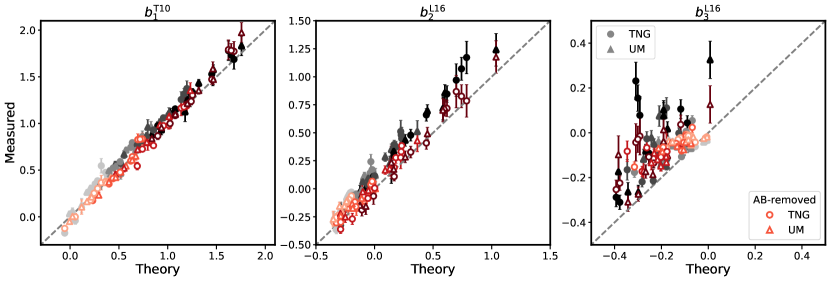
Figure 6: Our measured values of the bias parameters $b_{1}$, $b_{2}$, and $b_{3}$ compared to their theoretically motivated bias predictions for the original (grey) and assembly-bias-removed samples (red). The color intensity (light to dark) maps to the redshift (low to high). A 1:1 dashed line is plotted for reference.

To make these theoretical predictions, we compute the analytic bias as given in Equation 17. For $\frac{dn}{dM}$, we use the HMF of Tinker et al. (2010). For $\langle N(M)\rangle$, we empirically derive the HOD by extracting it from each of our TNG and UM galaxy samples. By construction of our shuffling procedure, as detailed in §5.1, this HOD is identical between the AB and AB-removed samples. For the LIMD halo bias parameters $b_{i,h}$, we use theoretically motivated fitting functions. First, we calculate the linear halo bias $b_{1,h}$ using the Tinker et al. (2010) fitting function:

$$b_{1,h}(\nu)=1-A\frac{\nu^{a}}{\nu^{a}+\delta_{c}^{a}}+B\nu^{b}+C\nu^{c},$$ (19)

where $\nu$ is the peak height and the parameters $\{A,a,B,b,C,c\}$ are defined in terms of the overdensity $\Delta=200$. Then, to compute the $b_{2,h}$ and $b_{3,h}$ halo bias parameters, we use the Lazeyras et al. (2016) fitting functions. These are given by

$$\begin{split}b_{2,h}\left(b_{1,h}\right)=\ &0.412-2.143b_{1,h}+0.929b_{1,h}^{2}+\\ &0.008b_{1,h}^{3}\end{split}$$ (20)

and

$$\begin{split}b_{3,h}\left(b_{1,h}\right)=-&1.028+7.646b_{1,h}-6.227b_{1,h}^{2}+\\ &0.912b_{1,h}^{3},\end{split}$$ (21)

respectively. We convert all three bias parameters into the Lagrangian frame using the co-evolution relations between Eulerian and Lagrangian bias. Finally, we integrate each component over the mass bins present in our selection. This allows us to make our theoretical prediction of the galaxy bias as a function of halo mass $M$ only, which we compare to our measured bias parameters for the original and AB-removed samples in Figure 6.

Here, we have plotted the original bias parameter measurements (filled gray markers) and the AB-removed bias parameter measurements (open red markers) against our theoretical predictions of the analytic bias. The original bias parameter measurements are larger than the theoretical predictions. This disagreement is stronger for the higher-order parameters but largely vanishes for the AB-removed measurements. This reflects the decreased value of the LIMD parameters on removing assembly bias in Figure 5. Although the original $b_{1}$ measurement was in reasonable agreement with the theory, we find overall that the AB-removed bias parameters match the theory predictions better than the original measurements. However, it should be noted that the AB-removed $b_{3}$ measurement still does not completely match the theory prediction.

To interpret the results of this comparison, we can apply the analytic bias prediction to our measured bias parameters. First we consider the original samples, which do include assembly bias. In this case, it is necessary to use a version of Equation 17 that incorporates this dependence. For now, let us simplistically assume that galaxy bias depends on a singular secondary halo property, which we call $X$:

$$b_{i}=\frac{1}{\bar{n}_{g}}\int dMdX\frac{d^{2}n}{dMdX}b_{i,h}(M,X)\langle N(M,X)\rangle,$$ (22)

where

$$\bar{n}_{g}=\int dMdX\frac{d^{2}n}{dMdX}\langle N(M,X)\rangle.$$ (23)

In this parameterization, the HMF $\frac{d^{2}n}{dMdX}$, HOD $\langle N(M,X)\rangle$, and halo bias $b_{i,h}(M,X)$ each have an additional dependence on some secondary halo property $X$, which does not appear in the original halo mass-only version of Equation 17. In this case, the original mass function can be written as $\frac{dn}{dM}=\frac{\bar{\rho}}{M}P(M)$, where $\bar{\rho}$ is the average dark matter density and $P(M)$ is the probability of a density fluctuation of mass M collapsing into a halo. By extension, $\frac{d^{2}n}{dMdX}=\frac{\bar{\rho}}{M}P(M,X)$, where we can use conditional probabilities to write $P(M,X)=P(M|X)P(X)$. As a result, simply marginalizing Equation 22 over the secondary halo property $X$ indeed results in an expression for galaxy bias that is only dependent on halo mass $M$, but this marginalized version of $b_{i}$ is not equivalent to the expression given in Equation 17. Given this inherent difference, it is no surprise that our original bias parameter measurements, which include assembly bias, differ from the theoretical prediction. This is especially true when considering the more realistic scenario of multiple secondary halo properties affecting galaxy clustering, such as age, spin, and concentration. As discussed in §5.1, it is this complex dependence of the HMF, HOD, and halo bias on various secondary halo properties that, when combined, boost our original bias parameter measurements relative to the theory prediction.

Now, it is helpful to consider the AB-removed bias parameter measurements: assuming that they match the theory prediction, this boost can be considered a signature of the strength of assembly bias. This signature appears to be weakest for the linear bias $b_{1}$ and strongest for the higher order parameters $b_{2}$ and $b_{3}$, implying that galaxy assembly bias may be difficult to detect when only considering linear galaxy bias. This is contrast to Zennaro et al. (2021)’s findings that $b_{1}$ is the most affected by assembly bias, even when considering $b_{2}$ and $b_{s^{2}}$ in much the same manner as our study: by comparing their results to those obtained from a mass-dependent HOD.

However, while we find that $b_{3}$ has a large boost relative to the theoretical prediction, this boost is reduced but not completely removed with removed assembly bias. This is particularly noteworthy when considering the $b_{3}(b_{1})$ relation. As discussed in §4.1.4, we find that our measurements of an “effective” cubic bias parameter are more positively biased than that of Lazeyras et al. (2016). Although the decrease in $b_{3}$ upon removing assembly bias cannot fully correct for the upward trend in our original measurements, it is partially mitigated. This could imply that, in addition to the missing cubic bias parameters in our expansion model, assembly bias is part of the reason for the deviation of our original measurements from the dark matter halo $b_{3}(b_{1})$ fit in Figure 3. It also means that it is important to consider what it means for our AB-removed bias parameter measurements to not match the theoretical prediction, as in the case of $b_{3}$.

To do this, we can use the form of analytic bias presented in Equation 17, as the only dependence of the AB-removed galaxy bias is on halo mass $M$. First, we consider $\frac{dn}{dM}$: we measure the abundance of halos in TNG and UM and verify that they both agree well with the Tinker et al. (2010) HMF. Second, we consider the HOD $\langle N(M)\rangle$, which has been preserved in the AB-removed samples through our shuffling procedure. This means that neither the HMF nor the HOD is a source of possible mismatch, leaving the halo bias $b_{i,h}(M)$. Any deviation of the AB-removed bias parameter measurements from the theoretical prediction must, therefore, be due to a discrepancy between the halo bias fitting function used and our measured value of the bias parameter. Assuming all fitting functions are correct, Figure 6 can thus be interpreted as a check of our galaxy bias parameter measurements.

We find that $b_{1}$ and $b_{2}$ pass this check, as the AB-removed bias parameters measurements match the theoretical galaxy bias prediction. However, $b_{3}$ does not pass this check, signifying that our measurement of $b_{3}$ is not truly the cubic LIMD bias parameter. This could be due to a combination of two effects: first, since we only include one cubic order bias parameter in our model, as given by Equation 6, our measurement of $b_{3}$ is a linear combination of the other missing cubic order bias parameters $b_{\delta s^{2}}$, $b_{s^{3}}$, and $b_{st}$. Second, our bias parameter measurements may suffer from not being able to successfully minimize our loss function, which is related to the variance of the stochasticity field $\bar{n}P_{\rm err}(k)$, as given by Equation 11. However, given that the other bias parameters have passed various checks, such as this analytic bias prediction for $b_{1}$ and $b_{2}$ in Figure 6, a consistency check of $b_{1}$ in Figure 10, and the convergence of $k_{\mathrm{max}}$ for all five bias parameters in Figure 11, this is unlikely. It is more probable that the deviation of the AB-removed $b_{3}$ measurements is simply a consequence of omitting the other cubic order bias parameters, as discussed in §4.1.4.

5.3 The degree of non-Poisson stochasticity

Having reported the measurements of bias parameters in our suite of samples and simulations, as well as the impact of galaxy assembly bias, we examine the stochastic power spectra $P_{\rm err}(k)$ that result from the stochasticity field ${\epsilon}(\mathbf{x})$ for each set of best-fit bias parameters $\hat{b}_{i}$. To calculate this stochasticity field, we generate a realization of the stochasticity field given by

$$\hat{\epsilon}(\mathbf{x})=\hat{\delta}_{g}(\mathbf{x})-\delta_{m}(\mathbf{x})-\sum_{i}\hat{b}_{i}\mathcal{O}_{i}(\mathbf{x}).$$ (24)

We do so for both the original and assembly-bias removed samples and assess the degree to which the dimensionless stochasticity spectrum $\bar{n}P_{\rm err}(k)$ deviates from the Poisson prediction of $\bar{n}P_{\rm err}=1$.

In previous work, Kokron et al. (2022) found that for LRGs sampled from three different HODs, across the redshift range $0\leq z\leq 1$, the deviations from stochasticity were small — on the order of at most 30% — except for a single sample in a single redshift bin. The samples we have constructed in this study allow us to expand on this discussion. Specifically, we can now understand whether the stochasticity of a galaxy sample changes significantly depending on galaxy type and whether different galaxy formation models conditioned on reproducing similar samples possess the same stochasticity, as we have seen for the case of galaxy bias in previous sections.

The small box size of $L=205\,h^{-1}{\rm Mpc}$ and lack of independent realizations to average over means that the individual spectra for a sample are noisier than those measured in Kokron et al. (2022). Thus, we instead fit a perturbative parametric form to each stochastic spectrum (Desjacques et al., 2018)

$$\bar{n}P_{\rm err}(k)=A_{0}+A_{1}\left(\frac{k}{k_{h}}\right)^{2},$$ (25)

where $A_{0}$ corresponds to the amplitude of the scale-independent contribution, $A_{1}$ modulates the first scale-dependent correction to the stochasticity, and $k_{h}$ is the cut-off scale for this expression of the stochasticity and is generically expected to be related to the characteristic scale of the 1-halo regime of the sample in question. If $A_{0}>1$, the sample’s stochasticity is super-Poisson, whereas if $A_{0}<1$, it is sub-Poisson. Mechanisms for the generation of sub-and-super Poisson stochasticity have been explored in-depth in past works, and we refer to them for a review (Hamaus et al., 2010; Baldauf et al., 2013; Kokron et al., 2022; Britt et al., 2024). We set $k_{h}=0.8\ h{\rm Mpc}^{-1}$ generically to report dimensionless values for $A_{1}$ in this work.

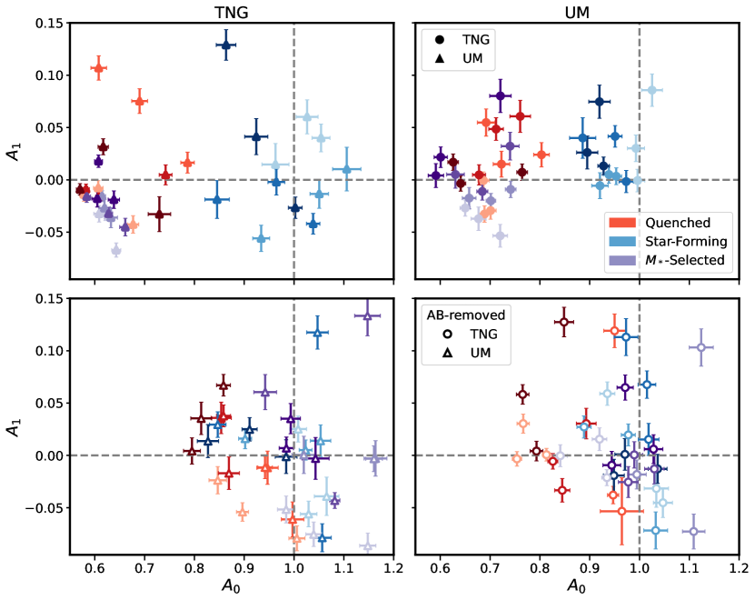
Figure 7: Measurements of the coefficients of the parameterized stochastic power spectrum of the samples considered in this work. $A_{0}=1$ and $A_{1}=0$ correspond to a spectrum derived from a Poisson shot-noise distributed sample. The top row shows measurements from TNG and UM, respectively, while the bottom row shows measurements from the versions of these samples with assembly bias removed as described in §5.1. The shading of the color corresponds to varying redshift bins, as in previous figures of this work.

To measure $A_{0}$ and $A_{1}$ for each sample, we fit Equation 25 to the measured stochastic power spectra $\bar{n}P_{\rm err}(k)$, assuming equal error-bars per $k$-bin. Using SciPy’s curve_fit function, we perform the fit within the wavenumbers $0.08\leq k/\ h{\rm Mpc}^{-1}<1.0$, although the results for $A_{0}$ are broadly insensitive to the exact $k_{\rm max}$ used. Finally, we use the covariance matrix returned by curve_fit to derive the uncertainty on each measurement of $A_{0}$ and $A_{1}$. These results are shown in Figure 7, where the measured $A_{0}$ and $A_{1}$ are plotted for quenched, star-forming and $M_{*}$-selected galaxies in both UM and TNG, as well as for the assembly-bias removed samples we define in §5.1.

We first focus on the stochasticity measurements for UM, shown in the upper right panel of Figure 7. They reveal a strong bimodality in the distribution of $A_{0}$ coefficients in the error power spectra of these galaxies, as the star-forming samples have power spectra very close to Poisson-distributed, occupying a narrow range of $\bar{n}P_{\rm err}(k)\approx[0.9,1.0]$. This is in contrast to both the $M_{*}$-selected and quenched samples, which all display strong sub-Poisson $\bar{n}P_{\rm err}(k)\approx[0.6,0.8]$. The most extreme degree of sub-Poisson stochasticity observed is still consistent with the results of Kokron et al. (2022). Although there are some detections of $A_{1}$ for these samples, the coefficients are very small and tend to be clustered around $A_{1}=0$. Note that due to the $k_{h}=0.8\ h{\rm Mpc}^{-1}$ normalization we have assumed, the inferred values of $A_{1}$ correspond to very small corrections to the flat stochasticities we have measured out to one-halo scales.

Contrasting the upper left panel of Figure 7 with the upper right reveals the differences in stochasticity between the two galaxy formation models we have considered in this work. Namely, we find that for similar galaxy samples, the TNG galaxies possess a larger scatter in both $A_{0}$ and $A_{1}$: the star-forming samples, in particular, exhibit a wide range of stochasticity in comparison to UM, while the higher values of $A_{1}$ in TNG could potentially correspond to the effects of explicitly implemented baryonic feedback in the stochasticity of the galaxy distribution, for example. However, the degree of stochasticity observed is still that of small and controllable deviations from the Poisson expectation, and the bimodality of stochasticity is equivalently apparent in both models. As a result, the measurements for UM and TNG remain consistent with the expectation that field-level stochasticities fit to a suitable bias model will be sub-Poisson for galaxies hosted in more massive halos, due to halo exclusion.

Finally, the last two panels in the bottom row of Figure 7 show the impact of removing assembly bias on the stochasticity of galaxy samples. Here, we observe that $A_{0}$ shifts to values closer to Poisson stochasticity for nearly all of the galaxy samples. This is somewhat intuitive, as the AB-removal procedure explicitly assigns satellite galaxies using a Poisson distribution. However, the collective shift of galaxies towards the Poisson regime points to a potential signature of assembly bias in the small-scale distribution of galaxies within halos. The values of $A_{0}$ inferred when we remove assembly bias from our samples are also closer in absolute magnitude to those seen in past work, which adopted an HOD to study galaxy stochasticity (Kokron et al., 2022). It is interesting that for these quenched samples a prominent impact of removing assembly bias is to reduce the degree of non-Poisson stochasticity. In the standard halo exclusion picture, the effect is solely dependent on the average mass of host halos Baldauf et al. (2013), and so we might expect that the AB-removed HOD would not qualitatively change this stochasticity.

This analysis of quenched galaxies in TNG and UM supports prior conclusions on the distribution of their stochasticity. The extension to star-forming galaxies also reveals that analyses of similar samples, such as ELGs, should be able to use Poisson shot noise as a strong guide for their expected stochasticity. As a last note, we do not find strong evidence for the redshift evolution of $A_{0}$ or $A_{1}$ in any of the samples.

5.4 Priors on $b_{i}$

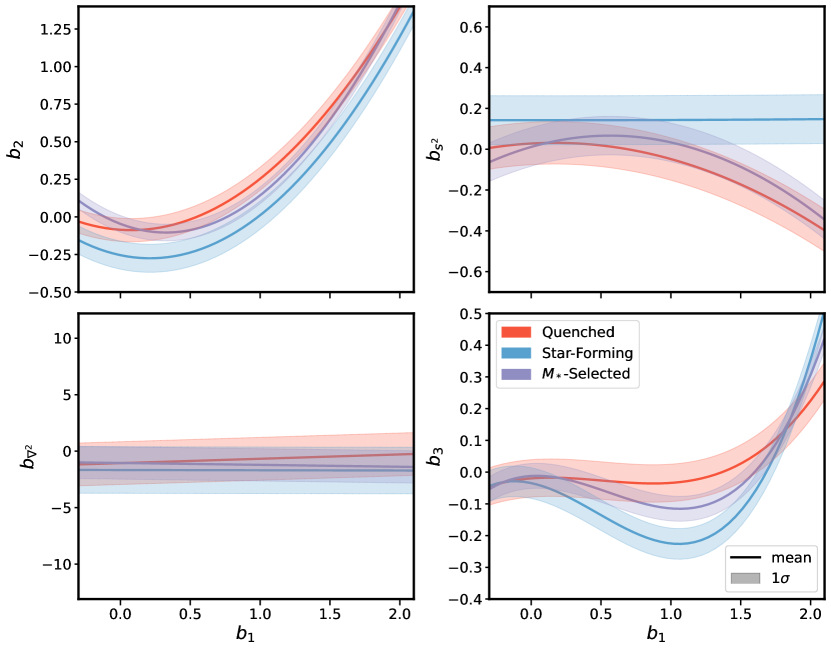
Figure 8: Gaussian priors for each of the bias parameter relations as a function of linear bias $b_{1}$. The bias parameter measurements are plotted for each sample of galaxies with and without AB in UM (triangles) and TNG (circles). Separate priors are set for the quenched (red), star-forming (blue), and the $M_{*}$-selected population (purple). The 1$\sigma$ standard deviation band is plotted around the best-fit polynomial, as labeled in each panel.

We present our priors on the $b_{2}(b_{1})$, $b_{s^{2}}(b_{1})$, $b_{\nabla^{2}}(b_{1})$ and $b_{3}(b_{1})$ bias relations in Figure 8. We set separate priors for each galaxy population (quenched, star-forming, and $M_{*}$-selected) and for each bias parameter due to our finding that the measured bias parameters are distinct between different galaxy types. In setting our priors, we include samples from both simulations (TNG, UM), all number density cuts (high, medium, low), and each redshift ($z=\{0.0,0.5,1.0,1.5\}$). We include the original and AB-removed galaxy samples to encompass as wide a range of viable galaxy formation physics as possible. This means that 48 galaxy samples are included when setting priors for each galaxy type in Figure 8. A detailed plot of the priors alongside these measurements is presented in Figure 13 of Appendix D.

Although we find outliers in the low-density cuts, as discussed in §4.2, these samples are, in fact, the most similar to realistic targets of galaxy clustering surveys. It is thus important that we do not exclude any of the galaxy samples and encompass the full range of measured bias parameters in our priors. For this reason, we have chosen to make Gaussian priors around a best-fit polynomial of varying degrees for each galaxy type. The degree of the polynomial fit corresponds to the order of the Lagrangian matter density contrast $\delta_{m}(\bf{k})$ for each bias field. We thus fit a quadratic function to the $b_{2}(b_{1})$ and $b_{s^{2}}(b_{1})$ relations, a line to the $b_{\nabla^{2}}(b_{1})$ relation, and a third degree polynomial to the $b_{3}(b_{1})$ relation.

$b_{i}(b_{1})$	Quenched	Star-Forming	$M_{*}$-Selected
$b_{2}(b_{1})$	$b_{2}=0.40b_{1}^{2}-0.06b_{1}-0.09$	$b_{2}=0.46b_{1}^{2}-0.20b_{1}-0.25$	$b_{2}=0.54b_{1}^{2}-0.35b_{1}-0.05$
	$\sigma_{b_{2}}=0.08$	$\sigma_{b_{2}}=0.09$	$\sigma_{b_{2}}=0.06$
$b_{s^{2}}(b_{1})$	$b_{s^{2}}=-0.12b_{1}^{2}+0.04b_{1}+0.03$	$b_{s^{2}}=0.001b_{1}^{2}-0.001b_{1}+0.14$	$b_{s^{2}}=-0.17b_{1}^{2}+0.20b_{1}+0.01$
	$\sigma_{b_{s^{2}}}=0.10$	$\sigma_{b_{s^{2}}}=0.12$	$\sigma_{b_{s^{2}}}=0.09$
$b_{\nabla^{2}}(b_{1})$	$b_{\nabla^{2}}=0.39b_{1}-1.06$	$b_{\nabla^{2}}=-0.02b_{1}-1.67$	$b_{\nabla^{2}}=-0.17b_{1}-1.05$
	$\sigma_{b_{\nabla^{2}}}=1.90$	$\sigma_{b_{\nabla^{2}}}=2.06$	$\sigma_{b_{\nabla^{2}}}=1.43$
$b_{3}(b_{1})$	$b_{3}=0.09b_{1}^{3}-0.14b_{1}^{2}+0.03b_{1}-0.02$	$b_{3}=0.24b_{1}^{3}-0.34b_{1}^{2}-0.09b_{1}-0.03$	$b_{3}=0.19b_{1}^{3}-0.32b_{1}^{2}+0.03b_{1}-0.01$
	$\sigma_{b_{3}}=0.06$	$\sigma_{b_{3}}=0.05$	$\sigma_{b_{3}}=0.04$

Table 1: Gaussian priors on the bias parameter relations $b_{2}(b_{1})$, $b_{s^{2}}(b_{1})$, $b_{\nabla^{2}}(b_{1})$, and $b_{3}(b_{1})$ for quenched, star-forming, and $M_{*}$-selected galaxies, defined by a best-fit line at $b_{i}(b_{1})$ and the $1\sigma$ standard deviation.

We make this fit using SciPy’s curve_fit function to carry out a weighted non-linear least-squares analysis. To ensure that our fit is as informed as possible, we take into account that some of our bias parameter measurements are less reliable than others. We do this by incorporating diagonals of the bias parameter covariance matrix, as given by Equation 15, on each measured bias parameter. We then calculate the standard deviation $\sigma_{b_{i}}$ of the 48 measured bias parameters from this best-fit line, and check separately that the spread of the bias parameters is indeed Gaussian around the best fit. The resulting best fit for each bias relation and galaxy type is plotted as a dashed line in each panel of Figure 13, while the standard deviation $\sigma_{b_{1}}$ is depicted as a shaded region around each best-fit curve. These best-fit polynomials and Gaussian $1\sigma$ standard deviations are listed for each bias parameter relation and each galaxy type in Table 1.

For the priors on the bias parameter relations to be most useful, we also set priors on $b_{1}$. Given the known evolution of the linear bias $b_{1}$ with redshift $z$ (Basilakos & Plionis, 2001; Nicola et al., 2024), we choose to set priors by fitting a curve to the time evolution of the linear bias parameter $b_{1}(z)$ that we measure in our samples. As we do for the bias parameter relations, we use SciPy’s curve_fit function to carry out a weighted non-linear least-squares analysis. However, to improve the interpretability of our results, we fit to the following modified function:

$$\begin{split}B_{1}(z)&=\frac{b_{1}^{E}(z)}{b_{1}^{E}(0)}\\ &=\frac{1+b_{1}(z)}{1+b_{1}(0)}.\end{split}$$ (26)

Rather than simply fitting to $b_{1}(z)$, we have made two changes here. First, to avoid zero-crossings of $b_{1}(z)$, we convert our measurement of the Lagrangian linear bias to the Eulerian linear bias via $b_{1}^{E}(z)=1+b_{1}(z).$ Second, to mitigate the vertical scatter due to the varying $b_{1}^{E}(z)$ relation among galaxy samples with different number density cuts, we have decided to define the fitting function relative to the value of the Eulerian linear bias $b_{1}^{E}(z)$ at $z=0$.

Although the redshift evolution of the first order bias $b_{1}(z)$ is commonly assumed to be linear in redshift $z$ using a model that conserves the number of galaxies over time (Matarrese et al., 1997), we choose to model $B_{1}(z)$ as a quadratic function. Primarily, under peak-background split, the linear bias can be modeled as

$$b_{1}=\frac{\nu^{2}-1}{\delta_{\mathrm{c}}}$$ (27)

using the Press–Schechter mass function (Mo & White, 1996). In an Einstein–de Sitter Universe, the linear growth factor scales as $D_{+}(z)\propto(1+z)^{-1}$, which means that we expect the linear bias to scale as $b_{1}\propto(1+z)^{2}$ for samples with $\nu(M,z)^{2}\gg 1$. This is exactly what we find, as we notice an improved fit to our measurements when modeling $B_{1}(z)$ as a quadratic, particularly in the $M_{*}$-selected sample. Additionally, there is a precedent for modeling the redshift evolution of $b_{1}(z)$ as a second-degree polynomial (Basilakos et al., 2008).

To obtain this fit, we thus weight the optimization function for $B_{1}(z)$ by the inverse of its error, as we do for the prior on the bias relations. However, because $B_{1}(z)$ depends on both $b_{1}(z)$ and $b_{1}(0)$, the error $\sigma_{b_{1}(z)}$ is not simply equivalent to $\sigma_{b_{1}(z)}$. Instead, we must propagate the uncertainty of $b_{1}(z)$ to the new function $B_{1}(z)$. The relative error is thus given by

$$\begin{split}\left(\frac{\sigma_{B_{1}(z)}}{B_{1}(z)}\right)^{2}\approx&\left(\frac{\sigma_{b_{1}(z)}}{b_{1}(z)}\right)^{2}+\left(\frac{\sigma_{b_{1}(0)}}{b_{1}(0)}\right)^{2}+\\ &2\left(\frac{\sigma_{b_{1}(z)}}{b_{1}(z)}\right)\left(\frac{\sigma_{b_{1}(0)}}{b_{1}(0)}\right)\rho_{b_{1}(z)b_{1}(0)}\\ \approx&\left(\frac{\sigma_{b_{1}(z)}}{b_{1}(z)}\right)^{2}+\left(\frac{\sigma_{b_{1}(0)}}{b_{1}(0)}\right)^{2},\end{split}$$ (28)

where we have assumed that the covariance $\rho_{b_{1}(z)b_{1}(0)}=0$.

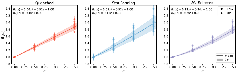
Figure 9: Gaussian priors for the time evolution of the linear bias $b_{1}$ relative to its value at $z=0$, parameterized as a fit to the mean $B_{1}(z)=\frac{1+b_{1}(z)}{1+b_{1}(0)}$. The bias parameter measurements are plotted for each sample of galaxies with and without AB in UM (triangles) and TNG (circles). Separate priors are set for the quenched (red), star-forming (blue), and the $M_{*}$-selected population (purple). The 1$\sigma$ standard deviation evolves linearly with redshift $z$ and is plotted as a shaded band around the best-fit polynomial, as labeled in each panel.

Using this method, we present our priors on the linear bias in Figure 9, where the best-fit line for $B_{1}(z)$ is plotted for quenched (red), star-forming (blue), and $M_{*}$-selected galaxies (purple) separately. Similar to Figure 8, each panel thus includes 48 bias parameter measurements across galaxy formation model (UM, TNG), redshift ($z=\{0.0,0.5,1.0,1.5\}$), number density cut (high, medium, low), and assembly bias (original, AB-removed). The modeled $1\sigma$ error of this fit is plotted as a shaded region around each line.

Quenched	Star-Forming	$M_{*}$-Selected
$B_{1}(z)=0.00z^{2}+0.57z+1.00$	$B_{1}(z)=0.05z^{2}+0.57z+1.00$	$B_{1}(z)=0.12z^{2}+0.34z+1.00$
$\sigma_{B_{1}}(z)=0.06z+0.00$	$\sigma_{B_{1}}(z)=0.11z+0.02$	$\sigma_{B_{1}}(z)=0.05z+0.00$

Table 2: Gaussian priors on the linear bias parameter $b_{1}$, parameterized via the best-fit mean to the function $B_{1}(z)=\frac{1+b_{1}(z)}{1+b_{1}(0)}$ for quenched, star-forming, and $M_{*}$-selected galaxies. The $1\sigma$ standard deviation evolves linearly as a function of redshift $z$.

Interestingly, we find that the error $\sigma_{B_{1}(z)}$ itself evolves as a function of redshift $z$. This can be seen directly in Figure 9, where the vertical scatter in the bias parameter measurements grows with redshift. To parameterize the time evolution of this scatter, we fit a line to the standard deviation of $B_{1}(z)$ at each redshift $z$, using SciPy’s curve_fit function to carry out an unweighted linear least-squares analysis. We find that this fit to $\sigma_{B_{1}(z)}$ describes the measured $\sigma_{B_{1}(z)}$ quite well, with the largest difference of $\Delta\sigma_{B_{1}(z)}\approx 0.1$ found in the star-forming population; our $\sigma_{B_{1}(z)}$ fit thus conservatively overestimates the standard deviation of the $B_{1}(z)$ fit. This fit to $\sigma_{B_{1}(z)}$, as well as $B_{1}(z)$, is listed in each panel of Figure 9, and is plotted as the standard deviation around the mean. Both fits are summarized in Table 2.

These priors on both $b_{i}(b_{1})$ and $B_{1}(z)$ may be directly adopted in future HEFT-based analyses that use galaxy clustering data to improve constraints on cosmological parameters (Hadzhiyska et al., 2021a; Chen et al., 2024; Sailer et al., 2024; Nicola et al., 2024). Because we find that the priors on quenched, star-forming, and $M_{*}$-selected galaxies behave distinctly from one another, we summarize these differences in the following sections. When applicable, we also provide guidance on their interpretation. For those who may prefer more conservative bounds, we also include in Appendix D a set of priors based on all of the 144 samples together rather than separating by galaxy type. These alternative priors on the bias relations $b_{i}(b_{1})$ are presented in Figure 14 and Table 4, while those on $B_{1}(z)$ are presented in Figure 15 and Table 5.

5.4.1 Quenched galaxies

The quenched galaxies are more positively biased in $b_{1}$ and $b_{3}$ than the star-forming galaxies at a given $b_{1}$. They are also slightly more biased in $b_{\nabla^{2}}(b_{1})$ than the star-forming galaxies. However, due to the large error bars, there is so much overlap between the two populations that any differences are negligible. In fact, all galaxy types, including the $M_{*}$-selected sample, are roughly constant at $b_{\nabla^{2}}(b_{1})\approx-1.$ Finally, although we allow for a second-degree dependence of $B_{1}(z)$ on redshift $z$, the time evolution of the linear bias for quenched galaxies remains very strongly linear.

Now, we consider the standard deviation of our priors: we find that the quenched galaxy population has much tighter bounds on all five bias parameters than the star-forming galaxy population. These tighter priors are slightly larger than, but still fairly comparable to the error in the $M_{*}$-selected sample. This suggests that there is less variation in modeling quenched and $M_{*}$-selected galaxies than star-forming galaxies for the galaxy formation models we consider.

5.4.2 Star-forming galaxies

We find that the star-forming galaxies are nearly constant in tidal bias at $b_{s^{2}}(b_{1})\approx 0.14$, while the quenched and $M_{*}$-selected samples follow a complex quadratic function that peaks at $b_{1}\approx 0.5$ and becomes increasingly more anti-biased. For the linear bias $b_{1}(z)$, we find that the star-forming sample has an even stronger dependence on redshift than the quenched galaxies, as both the slope of $B_{1}(z)$ and $\sigma_{B_{1}}(z)$ are larger than that of the star-forming galaxies. It should also be noted that while the error $\sigma_{B_{1}}(z)$ of star-forming galaxies appears linear, it is slightly quadratic.

This larger slope in $\sigma_{B_{1}}(z)$ means that the error in $B_{1}(z)$ for star-forming galaxies grows more rapidly with redshift than it does for both the quenched and $M_{*}$-selected populations. Overall, these wider priors for both the bias relations and time evolution of the linear bias of star-forming galaxies suggest that this galaxy population is the least agreed on by the models we consider and suffers from the most uncertainty in galaxy formation physics.

5.4.3 $M_{*}$-selected galaxies

The $M_{*}$-selected sample is characterized by properties that smoothly interpolate between the quenched and star-forming samples. This behavior is consistent with the fact that the halo occupation distribution for the $M_{*}$-selected sample is a linear combination of the quenched and star-forming galaxies. This means that the $M_{*}$-selected galaxies occupy a part of bias parameter space between the quenched and star-forming samples, a trend most evident in the prior for $b_{3}(b_{1})$. Here, we find that the shape of the prior is very similar to that of the star-forming sample, meaning that the $b_{3}$ of the $M_{*}$-selected sample evolves with linear bias $b_{1}$ in a similar manner to the star-forming sample. However, the former is shifted towards more positive values of $b_{3}$ than the latter, similar to the quenched sample.

Interestingly, we find that the $M_{*}$-selected sample has the tightest priors out of all the galaxy types that we consider. This is most evident in the $b_{2}(b_{1})$ and $b_{3}(b_{1})$ relation, as well as the linear bias. This suggests that the galaxy formation models we consider agree relatively more on how to model the stellar mass of galaxies than they do on the star-formation rate, which we use to distinguish between the quenched and star-forming population. This is partly reflected by the threshold cuts in $M_{*}$ and sSFR used to make the galaxy samples, listed in Table 3 in the Appendix. The difference in the threshold for sSFR makes it all the more compelling that the distinct parts of bias parameter space occupied by the different galaxy types are reproduced in both models, showing that the bias expansion is agnostic of the particular galaxy formation model.

Finally, it should be noted that although the quenched and star-forming galaxy populations are well-described by a Gaussian prior, the $M_{*}$-selected population has some outliers from the lowest number density cut in TNG; this is the same population of outliers noted previously in §4.2. Due to the outliers, the $B_{1}(z)$ fit is shifted slightly downwards of the overall $M_{*}$-selected measurements, meaning that the fit more accurately describes lower values of $B_{1}(z)$ for this sample. This results from the weighted fit that we perform on the bias parameter measurements, which preferentially prioritizes samples with smaller error bars. We see this clearly in Figure 9, as the error on $B_{1}(z)$ is highest for the $M_{*}$-selected samples that deviate the most from the fit.

5.5 Comparison with other work

As this paper was nearing submission, the work of Ivanov et al. (2024) was posted to the arXiv. They perform field-level fits in the “shifted operator basis” and Eulerian bias parameterization of Schmittfull et al. (2019) to samples of quenched and star-forming galaxies in two hydrodynamical simulations, as well as to explicitly parametric halo occupation distributions for LRG- and ELG-like samples. Where there is overlap, we broadly find that their results are consistent with those presented here. For example, this work also shows a split on $b_{2}(b_{1})$ for star-forming and quenched galaxies, has consistent results for real-space stochasticities, and shows a split between quenched and star-forming galaxies along the LLIMD prediction for the tidal bias parameter. Our work covers a wider redshift range and more distinct approaches to galaxy formation since, in addition to hydrodynamical simulations, we consider an empirical model tuned to a wide range of data and explicitly test for the impact of assembly bias. This allows us to demonstrate that the bias relations for galaxy populations at fixed number densities are only weakly sensitive to both redshift and to quite different galaxy formation prescriptions. This consistency with our work, despite different simulations and different methodologies for both generating the field-level forward model and fitting associated parameters, corroborates the robustness of our measurements and reported priors. Together, these papers give a coherent picture of the impact of uncertain galaxy formation physics on field-level bias models and provide further support for the importance of careful, analysis-specific work to quantify these uncertainties in the future.

6 Conclusions

In this work, we present direct, field-level comparisons of different models of galaxy formation using a second-order hybrid N-body Lagrangian perturbative bias expansion. We fit the bias expansion model to the density fields of galaxies from different models with the same initial conditions, while varying the number density, redshift, and type of galaxy included in our study. By using the same set of initial conditions, we can make a one-to-one comparison between models that include disparate approaches to galaxy formation. This allows us to estimate the range of bias parameters expected for typical galaxy samples over a range of reasonable, physically motivated models for galaxy formation, providing an essential ingredient for extracting the most precise cosmological information from current and future large galaxy surveys.

Specifically, we examine the UniverseMachine (UM), an empirical model of galaxy formation, and the IllustrisTNG (TNG) simulation. For each galaxy formation model, we make cuts on stellar mass ($M_{*}$) and specific star-formation rate to create catalogs of quenched and star-forming galaxies at a range of target number densities and redshifts ($z=\{0.0,0.5,1.0,1.5\}$). We also create a duplicate set of galaxy samples with assembly bias (AB) removed. These AB-removed samples can be considered an extension to the range of possible galaxy formation models. Consequently, by exploring the bias parameter space for a given galaxy population, we can investigate in detail not only the difference in bias between quenched and star-forming galaxies, but also quantify the uncertainty in these parameters due to changes in the galaxy formation model and uncertainties in the galaxy–halo connection.

Our primary findings are as follows:

1. We characterize the bias relations, which define the higher order bias parameters as a function of the linear bias ($b_{2}(b_{1})$, $b_{s^{2}}(b_{1})$, $b_{\nabla^{2}}(b_{1})$, $b_{3}(b_{1})$), for 144 different galaxy samples (Figure 3). We find general agreement between our bias parameter measurements and those in the literature that look at similar samples.

2. Star-forming and quenched galaxies occupy different parts of parameter space in the bias relations (Figures 3, 12). At fixed $b_{1}$, the $b_{2}$ and $b_{3}$ of quenched galaxies are larger than those of star-forming galaxies. In contrast, the opposite is generally true of the tidal bias: $b_{s^{2}}\leq 0$ for quenched galaxies, while $b_{s^{2}}\geq 0$ for their star-forming counterparts. $b_{\nabla^{2}}(b_{1})$ is the only bias relation for which we find no discernible differences between quenched and star-forming galaxies.

3. There is broad agreement between the bias relations for different models of galaxy formation (Figure 4). Low number density samples, which are currently less constrained by data and subject to more uncertain galaxy formation physics, exhibit more scatter (Figures 4, 12). There is also a wider range in the measured bias of star-forming galaxies, which generally tend to be more different between the UM and TNG models (Figures 10, 11).

4. Galaxy samples with realistic levels of assembly bias exceed analytic bias predictions that depend only on halo mass (Figure 6). They match these predictions for $b_{1}$ and $b_{2}$ after removing assembly bias, upon which $b_{2}$ and $b_{3}$ decrease, $b_{1}$ and $b_{s^{2}}$ remain unchanged, and $b_{\nabla^{2}}$ undergoes an orthogonal shift (Figure 5). This indicates that measured deviations from the analytic bias predictions may be viewed as a potential signature of assembly bias.

5. We quantify the degree of non-Poisson stochasticity in each galaxy sample (Figure 7). We find that star-forming samples are roughly Poisson, while the quenched and $M_{*}$-selected samples are sub-Poisson ($\bar{n}P_{\mathrm{err}}(k)\approx[0.6,0.8]$); this is expected because the latter are hosted in massive halos and experience more halo exclusion. Interestingly, we find that removing assembly bias shifts these samples from sub-Poisson to Poisson noise. This points to a potential signature of assembly bias in the one-halo regime.

6. We use our full set of samples to estimate the range of uncertainty in representative models of galaxy formation and set Gaussian priors on the bias relations (Figures 8, 9, 13, 14, 15). For each redshift, number density, and galaxy type (quenched, star-forming, $M_{*}$-selected), these priors encompass both galaxy formation models (TNG, UM) with and without assembly bias. While this is not a comprehensive marginalization over all possible galaxy formation models, it provides a reasonable assessment of the expected range given current understanding. These priors can be directly used in cosmological analyses that employ Lagrangian Perturbation Theory and Hybrid Effective Field Theory (HEFT).

The techniques we develop in this work allow us to directly compare any galaxy formation models using the bias expansion, as well as learn more about different galaxy populations. With this methodology in hand, there are several scientific directions we can now explore further. A natural first step is applying our analysis to other relevant targets of future surveys that require non-linear bias models to reliably extract cosmological parameters and demystify galaxy formation physics.

Compelling tracer populations include Lyman-break galaxies (LBGs), which are massive, star-forming galaxies selected by their photometric colors that can serve as a probe for the high-redshift ($z\approx[2,5]$) Universe, as well as inform science on dark energy, redshift-space distortions, and neutrino mass constraints (Wechsler et al., 2001; Park et al., 2016; Jose et al., 2017; Wilson & White, 2019; Newman et al., 2024). A similarly rare, high redshift tracer that would benefit from a robust model of non-linear bias is Lyman-alpha emitters (LAEs): young, star-forming galaxies residing in less massive halos than LBGs at $z\approx[2,6]$ (Sobacchi & Mesinger, 2015; Ebina & White, 2024; Ravi et al., 2024). These tracers provide exciting avenues forward, especially given the future DESI-II upgrades, which plan to target LBGs and LAEs (Schlegel et al., 2022).

Moving forward, it would be worthwhile to conduct such an analysis in a larger simulation volume, as the TNG300-1 Dark from the IllustrisTNG Project has a rather small box size of $L=205\ h{\rm Mpc}^{-1}$. This makes our results noisier than they would be in a larger box, as the error bars on our measurements scale inversely with volume (see Equation 15). An example of a more suitable simulation suite is the newest MilleniumTNG Project (Hernández-Aguayo et al., 2023), which pushes the IllustrisTNG galaxy formation model to a volume that matches the original Millennium simulation (Springel et al., 2005). Their largest run, MTNG740, spans a box size of $L=500\ h{\rm Mpc}^{-1}$: this is nearly a factor of 15 larger in volume than the IllustrisTNG box we have used in this work, meaning that the error bars on our bias parameter measurements would be reduced by a factor of about four. Yet another possibility is the FLAMINGO suite of hydrodynamical simulations (Schaye et al., 2023), which has dark-matter only counterparts for their boxes of size $L=1$ Gpc and $L=2.8$ Gpc; these would reduce our error bars by a factor of about 6 and 30, respectively. Such improvements would be particularly valuable for better understanding the noisiest bias parameters, $b_{s^{2}}$ and $b_{\nabla}^{2}$.

An additional avenue for reducing noise and increasing the accuracy of our bias parameter measurements is to investigate the impact of minimizing higher-order statistics of the stochasticity field, as in Schmittfull et al. (2019). Currently, we minimize the field-level variance, as Equation 11 shows, but it is possible to minimize, for example, the skewness or kurtosis simultaneously. It would be interesting to see the level of precision gained from this additional step.

Finally, although we have only lightly touched on assembly bias in this work, it is clear that it will be important for future galaxy clustering analyses to incorporate a dependence on secondary halo properties in their models of the galaxy–halo connection. This will be crucial for conducting accurate cosmological parameter inference. As a result, it would be interesting for a subsequent study to further investigate the effect of removing assembly bias on galaxy bias parameters, particularly how these changes compare among different models of galaxy formation and different galaxy types. It is especially important to understand how and why these changes occur, i.e., how exactly the halo mass function, halo occupation distribution function, and halo bias are influenced by certain secondary properties; this full study is beyond the scope of this work. A separate but related topic is the degree of non-stochasticity, as discussed in §5.3, which invites a full investigation into the impact of assembly bias on the stochasticity of our galaxy samples.

In sum, our findings show that quantifying the range of bias relations for physically motivated models of galaxy formation can provide tightened priors on bias relations, presenting an exciting avenue forward for HEFT-based cosmological constraint analyses, such as the recent work of Hadzhiyska et al. (2021a); Chen et al. (2024); Sailer et al. (2024); Nicola et al. (2024). The estimates provided here are particularly relevant for future DESI galaxy clustering measurements for LRGs and ELGs, as our galaxy selection and number density cuts are intended to mimic those targets. The techniques developed in this work will also be useful for maximizing information from other galaxy clustering data in the coming years, such as LSST, SPHEREx, Euclid, Roman, and beyond. Care should be taken to develop robust priors for such surveys tuned to the specific samples used for cosmological analyses; each sample will have different galaxy formation systematics, and each analysis will have different systematic requirements. Although we are not yet able to provide a true marginalization over all plausible models of galaxy formation, the modest range of bias relations that we find from a wide range of physically motivated galaxy formation models emphasizes the following: a robust understanding of galaxy formation can provide essential information that will significantly strengthen cosmological constraints from future surveys.

Data Availability

All data from the TNG300 simulation are available for download on the IllustrisTNG Project’s website. Access to other data underlying this paper is available upon reasonable request to the authors.

Appendix A Sample selection

$z$	Number Density/(10-4 $[\,h^{-1}{\rm Mpc}]^{-3}$)			Threshold
				Log($M_{*}$/$M_{\odot}$)		Log(sSFR/(year${}^{-1})$)
	Quenched	Star-Forming	$M_{*}$-Selected	TNG	UM	TNG	UM
	8.3	1.7	10	10.8	10.9	-11.7	-10.7
0	33	6.5	39	10.4	10.5	-11.3	-10.3
	57	11	68	10.2	10.3	-10.2	-10.1
	5.0	5.0	10	10.8	10.8	-11.7	-11.5
0.5	20	20	39	10.4	10.5	-11.5	-11.3
	34	34	68	10.1	10.3	-10.4	-11.2
	5.0	5.0	10	10.7	10.8	-10.9	-11.3
1	20	20	39	10.3	10.4	-10.2	-11.0
	34	34	68	10.0	10.2	-9.60	-9.80
	5	5	10	10.6	10.7	-10.3	-11.0
1.5	20	20	39	10.1	10.2	-9.40	-9.40
	34	34	68	9.90	9.90	-9.30	-9.10

Table 3: The number density of each galaxy population (quenched, star-forming, $M_{*}$-selected) at each redshift ($z=\{0.0,0.5,1.0,1.5\}$) used in this study, listed in increasing order. The stellar mass and specific star formation rate used to split each sample is also included under the column labeled “Threshold”.

As discussed in §3.2, we select the galaxy samples in this study by making cuts in $M_{*}$ and sSFR to achieve a certain target number density (low, medium, high) that is identical for each model (UM, TNG). The results of this sample selection are summarized in Table 3, where the total number density of each sample is listed under the $M_{*}$-selected column. This galaxy sample is split evenly between quenched and star-forming galaxies at each redshift $z$, aside from $z=0$, which is split such that the number density of quenched galaxies is five times as large as that of star-forming galaxies. This split in the $M_{*}$-selected population is made by selecting a threshold in sSFR, below which a galaxy is considered quenched and above which a galaxy is considered star-forming. The “Threshold” column of Table 3 lists the minimum $M_{*}$ that we include in our samples, as well as the sSFR at which we distinguish between quenched and star-forming galaxies.

It is noticeable that the $M_{*}$ cut is very similar between the TNG and UM models, which agree to 0.1 dex. We see more variation in the sSFR thresholds, of up to 1 dex. This variability in the sSFR threshold may be a reflection of the limitations of our straightforward sample selection method, which does not attempt to model galaxy colors or make cuts in color–magnitude space. However, our finding that the bias parameters are distinct between these two populations — something that is reproduced in both models — suggests that this is more likely due to a fundamental disagreement in what UM and TNG consider to be quenched and star-forming galaxies.

Appendix B Consistency with large-scale linear bias and running with $k_{\rm max}$

It is important to assess two assumptions that the bias estimator used in this work made: that we are performing unbiased estimates of bias parameters and that we have limited our measurements to scales where we do not observe strong running with the bias parameters. This is an important assumption, as in hybrid EFT, a running of the biases with $k_{\rm max}$ can be a sign of a potential breakdown of the bias expansion itself. This appendix concerns itself with validating these two assumptions.

To validate that our estimator recovers “unbiased” estimates of the bias parameters in full generality would require, for example, implementing separate-Universe simulations from which we can explicitly measure the LLIMD biases (as done in Lazeyras et al. (2016), which would require additional hydrodynamic and UniverseMachine simulations, beyond the scope of this work.

We thus opt, instead, to assess consistency between measurements of $b_{1}$ from the cross-correlation of the galaxy field with the dark matter field

$$\begin{split}b_{1}&=\lim_{k\to 0}\frac{\left\langle\delta_{g}(\textbf{k})\delta_{m}\left(\textbf{k}^{\prime}\right)\right\rangle}{\left\langle\delta_{m}(\textbf{k})\delta_{m}\left(\textbf{k}^{\prime}\right)\right\rangle}\\ &=\lim_{k\to 0}\frac{P_{gm}}{P_{mm}},\end{split}$$ (B1)

which is equivalent to the separate-universe definition of $b_{1}$.

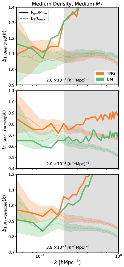
Figure 10: Consistency check of the large-scale approximation of the linear bias $b_{1}$ at $z=1$, computed via a ratio of the galaxy-matter cross-correlation power spectrum $P_{gm}$ to the matter-matter power spectrum $P_{mm}$. The approximation is plotted in solid lines for TNG (orange) and UM (green) as a function of scale $k$, while our measured $b_{1}(k_{\mathrm{max}})$ is plotted as a dashed line with shaded regions that show its theoretical error. The gray shaded region shows scales with $k_{\mathrm{max}}\geq 0.2\ h{\rm Mpc}^{-1}$ , which are discarded from our fit of the bias parameters.

This comparison is shown, for the medium density sample at $z=1$ in Figure 10. This spectrum is representative of all other densities and redshifts considered. The cross-spectrum ratio is plotted in bold lines for quenched, star-forming, and $M_{*}$-selected galaxies with a medium number density cut at $z=1$ in TNG (orange) and UM (green). Our measured values of $b_{1}$ as a function of $k_{\mathrm{max}}$ are plotted as a dashed line, with the theoretical error bars plotted as the filled region. The gray shaded space to the right of each panel shows the $k_{\mathrm{max}}=0.2\ h{\rm Mpc}^{-1}$ cut-off scale, beyond which includes modes that we do not include in our model.

Our measured values match the linear expectation of Equation B1 at large scales. Second, we find that our measured values of linear bias $b_{1}(k_{\mathrm{max}})$ only begin running with scale relative to their uncertainties for $k_{\mathrm{max}}>0.2\ h{\rm Mpc}^{-1}$. This check confirms that our estimates of $b_{1}$ are robust to at least $k_{\mathrm{max}}\sim 0.2\ h{\rm Mpc}^{-1}$, which is in contrast with the cross-spectrum estimates of $b_{1}$ that already deviate from a constant at $k>0.1\ h{\rm Mpc}^{-1}$.

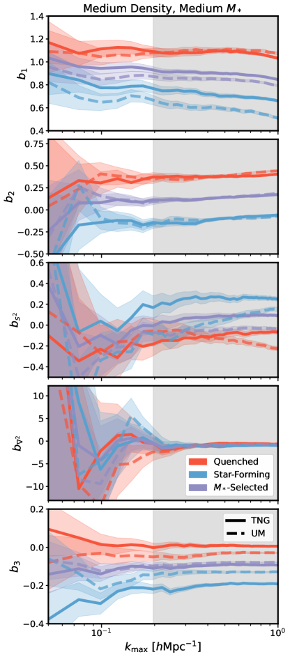
Figure 11: The bias parameter measurements $b_{1}$, $b_{2}$, $b_{s^{2}}$, $b_{\nabla^{2}}$, and $b_{3}$ at $z=1$ as a function of $k_{\mathrm{max}}$ for TNG (solid lines) and UM (dashed lines) for the quenched (red), star-forming (blue), and $M_{*}$-selected(purple) galaxy samples. Only the medium number density cut is shown. The theoretical error of the bias parameters is depicted by the shaded regions.

We also verify the lack of running up to $k_{\mathrm{max}}=0.2\ h{\rm Mpc}^{-1}$ for all five bias parameters, as shown in Figure 11. Here, a medium number density cut is shown at $z=1$ for quenched (red), star-forming (blue), and $M_{*}$-selected (purple) galaxies in UM (solid lines) and TNG (dashed lines). Our measured values of the bias parameters {$b_{1}$, $b_{2}$, $b_{s^{2}}$, $b_{\nabla^{2}}$, $b_{3}$} are plotted as a function of $k_{\mathrm{max}}$, with the estimated uncertainties plotted as the filled region. The gray shaded space to the right of each panel shows the $k_{\mathrm{max}}=0.2\ h{\rm Mpc}^{-1}$ cut-off scale, beyond which includes modes that we do not include in our model. We do note that the UM quenched and star-forming samples exhibit some large degree of running at scales beyond our cut-off, unlike the TNG measurements.

Like Figure 10, we see in Figure 11 that the bias parameters only begin running with scale for $k_{\mathrm{max}}>0.2\ h{\rm Mpc}^{-1}$, showing that this cut-off scale is appropriate for measuring each of the bias parameters. This acts as a validation check of our approach to describing the field-level distribution of galaxies using HEFT to second order in the Lagrangian bias expansion. It is also interesting to note that the larger scatter in the linear bias $b_{1}$ for star-forming galaxies, as discussed in §4.2, is apparent in both Figures 10 and 11. This wider scatter is reflected in our priors for the linear bias of star-forming galaxies. As discussed in §5.4.2 and shown in Figure 9, the standard deviation of $b_{1}(z)$ is larger for the star-forming galaxies than the other galaxy types, at all redshifts we consider.

Appendix C Impact of galaxy type

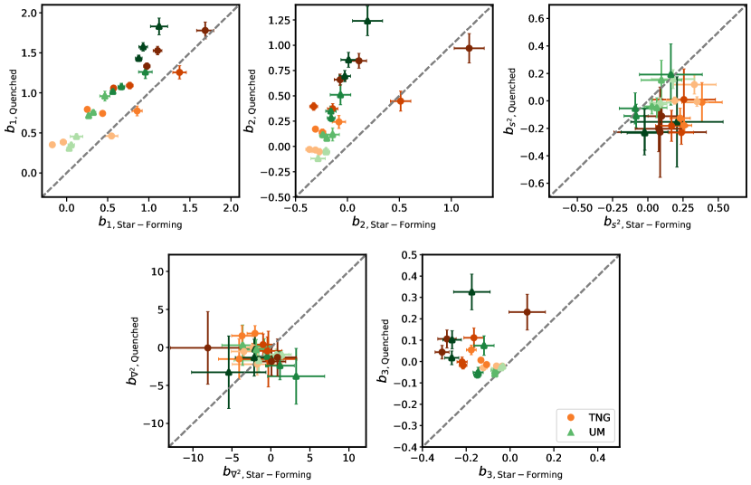
Figure 12: The bias parameter measurements of quenched galaxies in comparison to star-forming galaxies for samples at each number density and redshift ($z=\{0.0,0.5,1.0,1.5\}$) in TNG (orange circles) and UM (green triangles). The color intensity (light to dark) maps to the redshift (low to high). A 1:1 dashed line is plotted for reference.

Expanding upon the discussion in §4.2, we further investigate the impact of galaxy type on the bias parameter measurements by comparing the quenched and star-forming populations directly in Figure 12. We plot the bias measurements for matched quenched and star-forming samples at identical redshifts and number density cuts, in both UM (orange triangles) and TNG (gray circles). A 1:1 dashed line is plotted for reference.

Aside from some outliers in $b_{1}$ and $b_{2}$ for TNG, we see that none of the bias parameters follow this 1:1 relation between the two galaxy types. This supports our finding in §4.1 that quenched and star-forming galaxies occupy distinct parts of bias parameter space, with quenched galaxies being more heavily biased for the LIMD parameters $b_{1}$, $b_{2}$, and $b_{3}$. We find that the star-forming galaxies are more biased in $b_{s^{2}}$, a trend that is more pronounced in TNG than in UM. As discussed in §4.2, this is due to the higher value of $b_{s^{2}}$ for star-forming galaxies, and conversely lower value of $b_{s^{2}}$ for quenched galaxies, that we find in TNG compared to UM. In contrast, we find that there is no correlation in $b_{\nabla^{2}}$: both quenched and star-forming galaxies are centered around $b_{\nabla^{2}}\approx 0$, although it appears that there is more spread in the star-forming galaxies. This increased scatter is reflected in our priors; as listed in Table 1, the standard deviation $\sigma_{b_{\nabla}^{2}}$ is largest for star-forming galaxies in comparison to the other galaxy types.

Finally, similar to our findings in §4.2, we find that the few outliers that follow the 1:1 relation in $b_{1}$ and $b_{2}$ belong to the lowest number density sample. This is consistent with the wider scatter in $b_{1}$ and $b_{2}$ that we see in Figure 4. In Figure 11, however, we can determine that these low number density samples are from TNG, rather than UM. We thus find that TNG has a wider scatter in its measurements, and the largest discrepancies can be found in the highest-mass objects.

Appendix D Full Priors

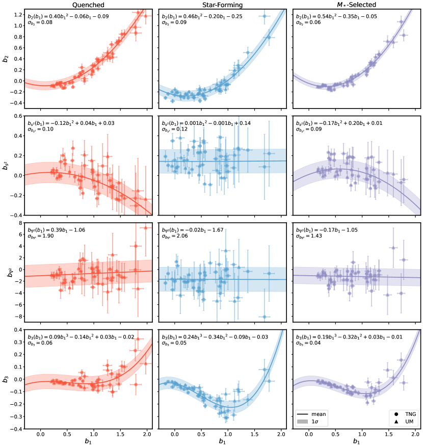
Figure 13: Gaussian priors for each of the bias parameter relations as a function of linear bias $b_{1}$. The bias parameter measurements are plotted for each sample of galaxies with and without AB in UM (triangles) and TNG (circles). Separate priors are set for the quenched (red), star-forming (blue), and the $M_{*}$-selected population (purple). The 1$\sigma$ standard deviation band is plotted around the best-fit polynomial, as labeled in each panel. This band characterizes the scatter between our range of galaxy formation prescriptions.

In a more detailed version of Figure 8, we present our priors on the bias parameter relations $b_{2}(b_{1})$, $b_{s^{2}}(b_{1})$, $b_{\nabla^{2}}(b_{1})$ and $b_{3}(b_{1})$ in Figure 13. The best-fit curve is plotted as a solid line, and the shaded region depicts the standard deviation around this mean. The priors are identical to those shown in Figure 8, but for readability, we have separated the quenched (red), star-forming (blue), and $M_{*}$-selected (purple) samples into different columns. For full transparency, we also elect to show all of the bias parameter measurements for which we make the best-fit curve. These are represented by circle and triangle markers for TNG and UM, respectively, and span all redshifts ($z=\{0.0,0.5,1.0,1.5\}$) and number density cuts (high, medium, low). Both the original and AB-removed measurements are also included in each fit, for a total of 48 samples in each panel. This choice was made so that our analysis could span as full a range of galaxy formation physics as possible.

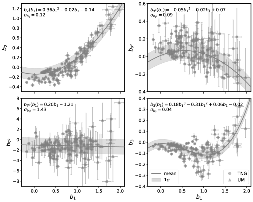
Figure 14: Conservative Gaussian priors for each of the bias parameter relations as a function of linear bias $b_{1}$. The bias parameter measurements are plotted for each sample of galaxies with and without AB in UM (triangles) and TNG (circles). Priors are set for the all samples of galaxies together, including the quenched, star-forming, and the $M_{*}$-selected population. The 1$\sigma$ standard deviation band is plotted around the best-fit polynomial, as labeled in each panel.

$b_{i}(b_{1})$	All Galaxies
$b_{2}(b_{1})$	$b_{2}=0.36b_{1}^{2}-0.02b_{1}-0.14$
	$\sigma_{b_{2}}=0.12$
$b_{s^{2}}(b_{1})$	$b_{s^{2}}=-0.05b_{1}^{2}-0.02b_{1}+0.07$
	$\sigma_{b_{s^{2}}}=0.09$
$b_{\nabla^{2}}(b_{1})$	$b_{\nabla^{2}}=0.20b_{1}-1.21$
	$\sigma_{b_{\nabla^{2}}}=1.43$
$b_{3}(b_{1})$	$b_{3}=0.18b_{1}^{3}-0.31b_{1}^{2}+0.06b_{1}-0.02$
	$\sigma_{b_{3}}=0.04$

Table 4: Conservative Gaussian priors on the bias parameter relations $b_{2}(b_{1})$, $b_{s^{2}}(b_{1})$, $b_{\nabla^{2}}(b_{1})$, and $b_{3}(b_{1})$ for all samples of galaxies together, including the quenched, star-forming, and $M_{*}$-selected population. Priors are defined by a best-fit line at $b_{i}(b_{1})$ and the $1\sigma$ standard deviation.

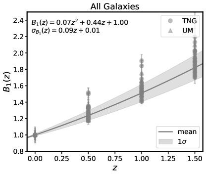
Figure 15: Conservative Gaussian priors for the time evolution of the linear bias $b_{1}$ relative to its value at $z=0$, parameterized as a fit to the mean $B_{1}(z)=\frac{1+b_{1}(z)}{1+b_{1}(0)}$. The bias parameter measurements are plotted for each sample of galaxies with and without AB in UM (triangles) and TNG (circles). Priors are set for all of the samples of galaxies together, including the quenched, star-forming, and the $M_{*}$-selected population. The 1$\sigma$ standard deviation evolves linearly with redshift $z$ and is plotted as a shaded band around the best-fit polynomial, as labeled in each panel.

All Galaxies
$B_{1}(z)=0.07z^{2}+0.44z+1.00$
$\sigma_{B_{1}}(z)=0.09z+0.01$

Table 5: Conservative Gaussian priors on the linear bias parameter $b_{1}$, parameterized via the best-fit mean to the function $B_{1}(z)=\frac{1+b_{1}(z)}{1+b_{1}(0)}$ for all samples of galaxies together, including the quenched, star-forming, and $M_{*}$-selected population. The $1\sigma$ standard deviation evolves linearly as a function of redshift $z$.

We also present in Figure 14 an alternative, more conservative set of priors to those in Figures 8, 9, and 13. Instead of separating the samples by galaxy type, we treat all of the galaxy samples together and present one set of priors for all of the data, using the same method detailed in §5.4. We include these 144 data samples in the figure for comparison. The best-fit mean and $1\sigma$ standard deviation are listed in each panel of Figure 14, as well as in Table 4. We present the corresponding priors in $B_{1}(z)$ in Figure 15 and Table 5. These priors may be more suitable for those desiring a less restrictive set of bounds in a HEFT-based cosmological analysis than the sample-specific priors presented in this work.

References

- Abidi & Baldauf (2018) Abidi, M. M., & Baldauf, T. 2018, Journal of Cosmology and Astroparticle Physics, 2018, 029–029, doi: 10.1088/1475-7516/2018/07/029
- Akeson et al. (2019) Akeson, R., Armus, L., Bachelet, E., et al. 2019, arXiv e-prints, arXiv:1902.05569, doi: 10.48550/arXiv.1902.05569
- Akitsu (2024) Akitsu, K. 2024, arXiv e-prints, arXiv:2410.08998, doi: 10.48550/arXiv.2410.08998
- Angulo et al. (2008) Angulo, R. E., Baugh, C. M., & Lacey, C. G. 2008, MNRAS, 387, 921, doi: 10.1111/j.1365-2966.2008.13304.x
- Artale et al. (2018) Artale, M. C., Zehavi, I., Contreras, S., & Norberg, P. 2018, MNRAS, 480, 3978, doi: 10.1093/mnras/sty2110
- Baldauf et al. (2016) Baldauf, T., Schaan, E., & Zaldarriaga, M. 2016, J. Cosmology Astropart. Phys, 2016, 017, doi: 10.1088/1475-7516/2016/03/017
- Baldauf et al. (2013) Baldauf, T., Seljak, U., Smith, R. E., Hamaus, N., & Desjacques, V. 2013, Physical Review D, 88, doi: 10.1103/physrevd.88.083507
- Barreira et al. (2020) Barreira, A., Cabass, G., Schmidt, F., Pillepich, A., & Nelson, D. 2020, J. Cosmology Astropart. Phys, 2020, 013, doi: 10.1088/1475-7516/2020/12/013
- Barreira et al. (2021) Barreira, A., Lazeyras, T., & Schmidt, F. 2021, J. Cosmology Astropart. Phys, 2021, 029, doi: 10.1088/1475-7516/2021/08/029
- Basilakos & Plionis (2001) Basilakos, S., & Plionis, M. 2001, ApJ, 550, 522, doi: 10.1086/319797
- Basilakos et al. (2008) Basilakos, S., Plionis, M., & Ragone-Figueroa, C. 2008, ApJ, 678, 627, doi: 10.1086/586725
- Baugh et al. (1999) Baugh, C. M., Benson, A. J., Cole, S., Frenk, C. S., & Lacey, C. G. 1999, MNRAS, 305, L21, doi: 10.1046/j.1365-8711.1999.02590.x
- Baumann et al. (2012) Baumann, D., Nicolis, A., Senatore, L., & Zaldarriaga, M. 2012, J. Cosmology Astropart. Phys, 2012, 051, doi: 10.1088/1475-7516/2012/07/051
- Behroozi et al. (2019) Behroozi, P., Wechsler, R. H., Hearin, A. P., & Conroy, C. 2019, MNRAS, 488, 3143, doi: 10.1093/mnras/stz1182
- Benson et al. (2000) Benson, A. J., Cole, S., Frenk, C. S., Baugh, C. M., & Lacey, C. G. 2000, MNRAS, 311, 793, doi: 10.1046/j.1365-8711.2000.03101.x
- Berlind & Weinberg (2002) Berlind, A. A., & Weinberg, D. H. 2002, ApJ, 575, 587, doi: 10.1086/341469
- Bernardeau et al. (2002) Bernardeau, F., Colombi, S., Gaztañaga, E., & Scoccimarro, R. 2002, Phys. Rep., 367, 1, doi: 10.1016/S0370-1573(02)00135-7
- Bose et al. (2019) Bose, S., Eisenstein, D. J., Hernquist, L., et al. 2019, MNRAS, 490, 5693, doi: 10.1093/mnras/stz2546
- Bose et al. (2023) Bose, S., Hadzhiyska, B., Barrera, M., et al. 2023, MNRAS, 524, 2579, doi: 10.1093/mnras/stad1097
- Britt et al. (2024) Britt, D., Gruen, D., Friedrich, O., Yuan, S., & Ried Guachalla, B. 2024, A&A, 689, A253, doi: 10.1051/0004-6361/202450266
- Carrasco et al. (2012) Carrasco, J. J. M., Hertzberg, M. P., & Senatore, L. 2012, Journal of High Energy Physics, 2012, 82, doi: 10.1007/JHEP09(2012)082
- Carrilho et al. (2023) Carrilho, P., Moretti, C., & Pourtsidou, A. 2023, J. Cosmology Astropart. Phys, 2023, 028, doi: 10.1088/1475-7516/2023/01/028
- Chen et al. (2024) Chen, S., DeRose, J., Zhou, R., et al. 2024, arXiv e-prints, arXiv:2407.04795, doi: 10.48550/arXiv.2407.04795
- Cole & Kaiser (1989) Cole, S., & Kaiser, N. 1989, MNRAS, 237, 1127, doi: 10.1093/mnras/237.4.1127
- Collaboration et al. (2024a) Collaboration, D., Adame, A. G., Aguilar, J., et al. 2024a, DESI 2024 VI: Cosmological Constraints from the Measurements of Baryon Acoustic Oscillations. https://arxiv.org/abs/2404.03002
- Collaboration et al. (2024b) —. 2024b, DESI 2024 V: Full-Shape Galaxy Clustering from Galaxies and Quasars. https://arxiv.org/abs/2411.12021
- Contreras et al. (2019) Contreras, S., Zehavi, I., Padilla, N., et al. 2019, MNRAS, 484, 1133, doi: 10.1093/mnras/stz018
- Crain et al. (2009) Crain, R. A., Theuns, T., Dalla Vecchia, C., et al. 2009, Monthly Notices of the Royal Astronomical Society, 399, 1773, doi: 10.1111/j.1365-2966.2009.15402.x
- Croton et al. (2007) Croton, D. J., Gao, L., & White, S. D. M. 2007, MNRAS, 374, 1303, doi: 10.1111/j.1365-2966.2006.11230.x
- Dalal et al. (2008) Dalal, N., White, M., Bond, J. R., & Shirokov, A. 2008, ApJ, 687, 12, doi: 10.1086/591512
- Davis et al. (1985) Davis, M., Efstathiou, G., Frenk, C. S., & White, S. D. M. 1985, ApJ, 292, 371, doi: 10.1086/163168
- DESI Collaboration et al. (2016) DESI Collaboration, Aghamousa, A., Aguilar, J., et al. 2016, arXiv e-prints, arXiv:1611.00036, doi: 10.48550/arXiv.1611.00036
- Desjacques et al. (2018) Desjacques, V., Jeong, D., & Schmidt, F. 2018, Phys. Rep., 733, 1, doi: 10.1016/j.physrep.2017.12.002
- Dolag et al. (2009) Dolag, K., Borgani, S., Murante, G., & Springel, V. 2009, MNRAS, 399, 497, doi: 10.1111/j.1365-2966.2009.15034.x
- Donald-McCann et al. (2023) Donald-McCann, J., Gsponer, R., Zhao, R., Koyama, K., & Beutler, F. 2023, MNRAS, 526, 3461, doi: 10.1093/mnras/stad2957
- Doré et al. (2014) Doré, O., Bock, J., Ashby, M., et al. 2014, arXiv e-prints, arXiv:1412.4872, doi: 10.48550/arXiv.1412.4872
- Ebina & White (2024) Ebina, H., & White, M. 2024, J. Cosmology Astropart. Phys, 2024, 052, doi: 10.1088/1475-7516/2024/06/052
- Eifler et al. (2021) Eifler, T., Miyatake, H., Krause, E., et al. 2021, MNRAS, 507, 1746, doi: 10.1093/mnras/stab1762
- Gao et al. (2005) Gao, L., Springel, V., & White, S. D. M. 2005, MNRAS, 363, L66, doi: 10.1111/j.1745-3933.2005.00084.x
- Hadzhiyska et al. (2020) Hadzhiyska, B., Bose, S., Eisenstein, D., Hernquist, L., & Spergel, D. N. 2020, MNRAS, 493, 5506, doi: 10.1093/mnras/staa623
- Hadzhiyska et al. (2021a) Hadzhiyska, B., García-García, C., Alonso, D., Nicola, A., & Slosar, A. 2021a, J. Cosmology Astropart. Phys, 2021, 020, doi: 10.1088/1475-7516/2021/09/020
- Hadzhiyska et al. (2021b) Hadzhiyska, B., Liu, S., Somerville, R. S., et al. 2021b, MNRAS, 508, 698, doi: 10.1093/mnras/stab2564
- Hadzhiyska et al. (2021c) Hadzhiyska, B., Tacchella, S., Bose, S., & Eisenstein, D. J. 2021c, MNRAS, 502, 3599, doi: 10.1093/mnras/stab243
- Hadzhiyska et al. (2023) Hadzhiyska, B., Eisenstein, D., Hernquist, L., et al. 2023, MNRAS, 524, 2507, doi: 10.1093/mnras/stad731
- Hamaus et al. (2010) Hamaus, N., Seljak, U., Desjacques, V., Smith, R. E., & Baldauf, T. 2010, Physical Review D, 82, doi: 10.1103/physrevd.82.043515
- Hand et al. (2018) Hand, N., Feng, Y., Beutler, F., et al. 2018, AJ, 156, 160, doi: 10.3847/1538-3881/aadae0
- Hearin et al. (2016) Hearin, A. P., Zentner, A. R., van den Bosch, F. C., Campbell, D., & Tollerud, E. 2016, MNRAS, 460, 2552, doi: 10.1093/mnras/stw840
- Hernández-Aguayo et al. (2023) Hernández-Aguayo, C., Springel, V., Pakmor, R., et al. 2023, MNRAS, 524, 2556, doi: 10.1093/mnras/stad1657
- Holm et al. (2023) Holm, E. B., Herold, L., Simon, T., et al. 2023, Phys. Rev. D, 108, 123514, doi: 10.1103/PhysRevD.108.123514
- Ivanov et al. (2024a) Ivanov, M. M., Cuesta-Lazaro, C., Mishra-Sharma, S., Obuljen, A., & Toomey, M. W. 2024a, Phys. Rev. D, 110, 063538, doi: 10.1103/PhysRevD.110.063538
- Ivanov et al. (2024b) —. 2024b, arXiv e-prints, arXiv:2402.13310, doi: 10.48550/arXiv.2402.13310
- Ivanov et al. (2024c) Ivanov, M. M., Obuljen, A., Cuesta-Lazaro, C., & Toomey, M. W. 2024c, arXiv e-prints, arXiv:2409.10609, doi: 10.48550/arXiv.2409.10609
- Ivanov et al. (2024) Ivanov, M. M., Cuesta-Lazaro, C., Obuljen, A., et al. 2024, The Millennium and Astrid galaxies in effective field theory: comparison with galaxy-halo connection models at the field level. https://arxiv.org/abs/2412.01888
- Ivezić et al. (2019) Ivezić, Ž., Kahn, S. M., Tyson, J. A., et al. 2019, The Astrophysical Journal, 873, 111, doi: 10.3847/1538-4357/ab042c
- Jose et al. (2017) Jose, C., Baugh, C. M., Lacey, C. G., & Subramanian, K. 2017, MNRAS, 469, 4428, doi: 10.1093/mnras/stx1014
- Kaiser (1984) Kaiser, N. 1984, ApJ, 284, L9, doi: 10.1086/184341
- Kauffmann et al. (2013) Kauffmann, G., Li, C., Zhang, W., & Weinmann, S. 2013, MNRAS, 430, 1447, doi: 10.1093/mnras/stt007
- Kawinwanichakij et al. (2016) Kawinwanichakij, L., Quadri, R. F., Papovich, C., et al. 2016, ApJ, 817, 9, doi: 10.3847/0004-637X/817/1/9
- Kokron et al. (2021) Kokron, N., DeRose, J., Chen, S.-F., White, M., & Wechsler, R. H. 2021, MNRAS, 505, 1422, doi: 10.1093/mnras/stab1358
- Kokron et al. (2022) Kokron, N., DeRose, J., Chen, S.-F., White, M., & Wechsler, R. H. 2022, Monthly Notices of the Royal Astronomical Society, 514, 2198, doi: 10.1093/mnras/stac1420
- Krause et al. (2017) Krause, E., Eifler, T. F., Zuntz, J., et al. 2017, arXiv e-prints, arXiv:1706.09359, doi: 10.48550/arXiv.1706.09359
- Laureijs et al. (2011) Laureijs, R., Amiaux, J., Arduini, S., et al. 2011, arXiv e-prints, arXiv:1110.3193, doi: 10.48550/arXiv.1110.3193
- Lazeyras et al. (2021) Lazeyras, T., Barreira, A., & Schmidt, F. 2021, J. Cosmology Astropart. Phys, 2021, 063, doi: 10.1088/1475-7516/2021/10/063
- Lazeyras et al. (2023) Lazeyras, T., Barreira, A., Schmidt, F., & Desjacques, V. 2023, J. Cosmology Astropart. Phys, 2023, 023, doi: 10.1088/1475-7516/2023/01/023
- Lazeyras et al. (2017) Lazeyras, T., Musso, M., & Schmidt, F. 2017, J. Cosmology Astropart. Phys, 2017, 059, doi: 10.1088/1475-7516/2017/03/059
- Lazeyras & Schmidt (2018) Lazeyras, T., & Schmidt, F. 2018, J. Cosmology Astropart. Phys, 2018, 008, doi: 10.1088/1475-7516/2018/09/008
- Lazeyras & Schmidt (2019) —. 2019, J. Cosmology Astropart. Phys, 2019, 041, doi: 10.1088/1475-7516/2019/11/041
- Lazeyras et al. (2016) Lazeyras, T., Wagner, C., Baldauf, T., & Schmidt, F. 2016, J. Cosmology Astropart. Phys, 2016, 018, doi: 10.1088/1475-7516/2016/02/018
- Lucie-Smith et al. (2023) Lucie-Smith, L., Barreira, A., & Schmidt, F. 2023, MNRAS, 524, 1746, doi: 10.1093/mnras/stad2003
- MacCrann et al. (2020) MacCrann, N., Blazek, J., Jain, B., & Krause, E. 2020, MNRAS, 491, 5498, doi: 10.1093/mnras/stz2761
- Mansfield & Kravtsov (2020) Mansfield, P., & Kravtsov, A. V. 2020, MNRAS, 493, 4763, doi: 10.1093/mnras/staa430
- Mao et al. (2018) Mao, Y.-Y., Zentner, A. R., & Wechsler, R. H. 2018, MNRAS, 474, 5143, doi: 10.1093/mnras/stx3111
- Martig et al. (2009) Martig, M., Bournaud, F., Teyssier, R., & Dekel, A. 2009, ApJ, 707, 250, doi: 10.1088/0004-637X/707/1/250
- Matarrese et al. (1997) Matarrese, S., Coles, P., Lucchin, F., & Moscardini, L. 1997, Monthly Notices of the Royal Astronomical Society, 286, 115, doi: 10.1093/mnras/286.1.115
- Matsubara (2008) Matsubara, T. 2008, Phys. Rev. D, 77, 063530, doi: 10.1103/PhysRevD.77.063530
- Maus et al. (2023) Maus, M., Chen, S.-F., & White, M. 2023, J. Cosmology Astropart. Phys, 2023, 005, doi: 10.1088/1475-7516/2023/06/005
- Mo & White (1996) Mo, H. J., & White, S. D. M. 1996, MNRAS, 282, 347, doi: 10.1093/mnras/282.2.347
- Modi et al. (2017) Modi, C., Castorina, E., & Seljak, U. 2017, MNRAS, 472, 3959, doi: 10.1093/mnras/stx2148
- Modi et al. (2020) Modi, C., Chen, S.-F., & White, M. 2020, MNRAS, 492, 5754, doi: 10.1093/mnras/staa251
- Nelson et al. (2021) Nelson, D., Springel, V., Pillepich, A., et al. 2021, The IllustrisTNG Simulations: Public Data Release. https://arxiv.org/abs/1812.05609
- Newman et al. (2024) Newman, A. B., Qezlou, M., Chartab, N., et al. 2024, ApJ, 961, 27, doi: 10.3847/1538-4357/ad0896
- Nicola et al. (2024) Nicola, A., Hadzhiyska, B., Findlay, N., et al. 2024, J. Cosmology Astropart. Phys, 2024, 015, doi: 10.1088/1475-7516/2024/02/015
- Paranjape & Padmanabhan (2017) Paranjape, A., & Padmanabhan, N. 2017, MNRAS, 468, 2984, doi: 10.1093/mnras/stx659
- Park et al. (2016) Park, J., Kim, H.-S., Wyithe, J. S. B., et al. 2016, MNRAS, 461, 176, doi: 10.1093/mnras/stw1316
- Park et al. (2021) Park, Y., Rozo, E., & Krause, E. 2021, Phys. Rev. Lett., 126, 021301, doi: 10.1103/PhysRevLett.126.021301
- Ravi et al. (2024) Ravi, J., Hadzhiyska, B., White, M., Hernquist, L., & Bose, S. 2024, arXiv e-prints, arXiv:2403.02414, doi: 10.48550/arXiv.2403.02414
- Reid et al. (2010) Reid, B. A., Verde, L., Dolag, K., Matarrese, S., & Moscardini, L. 2010, J. Cosmology Astropart. Phys, 2010, 013, doi: 10.1088/1475-7516/2010/07/013
- Ried Guachalla et al. (2024) Ried Guachalla, B., Britt, D., Gruen, D., & Friedrich, O. 2024, arXiv e-prints, arXiv:2405.00261, doi: 10.48550/arXiv.2405.00261
- Rubira & Schmidt (2023) Rubira, H., & Schmidt, F. 2023, Galaxy bias renormalization group. https://arxiv.org/abs/2307.15031
- Sailer et al. (2024) Sailer, N., Kim, J., Ferraro, S., et al. 2024, arXiv e-prints, arXiv:2407.04607, doi: 10.48550/arXiv.2407.04607
- Saito et al. (2014) Saito, S., Baldauf, T., Vlah, Z., et al. 2014, Phys. Rev. D, 90, 123522, doi: 10.1103/PhysRevD.90.123522
- Salcedo et al. (2018) Salcedo, A. N., Maller, A. H., Berlind, A. A., et al. 2018, MNRAS, 475, 4411, doi: 10.1093/mnras/sty109
- Sato-Polito et al. (2019) Sato-Polito, G., Montero-Dorta, A. D., Abramo, L. R., Prada, F., & Klypin, A. 2019, MNRAS, 487, 1570, doi: 10.1093/mnras/stz1338
- Schaye et al. (2023) Schaye, J., Kugel, R., Schaller, M., et al. 2023, MNRAS, 526, 4978, doi: 10.1093/mnras/stad2419
- Schlegel et al. (2022) Schlegel, D. J., Ferraro, S., Aldering, G., et al. 2022, arXiv e-prints, arXiv:2209.03585, doi: 10.48550/arXiv.2209.03585
- Schmittfull et al. (2019) Schmittfull, M., Simonović, M., Assassi, V., & Zaldarriaga, M. 2019, Phys. Rev. D, 100, 043514, doi: 10.1103/PhysRevD.100.043514
- Schmittfull et al. (2019) Schmittfull, M., Simonović, M., Assassi, V., & Zaldarriaga, M. 2019, Physical Review D, 100, doi: 10.1103/physrevd.100.043514
- Scoccimarro et al. (2001) Scoccimarro, R., Sheth, R. K., Hui, L., & Jain, B. 2001, ApJ, 546, 20, doi: 10.1086/318261
- Seljak (2000) Seljak, U. 2000, MNRAS, 318, 203, doi: 10.1046/j.1365-8711.2000.03715.x
- Senatore (2015) Senatore, L. 2015, Journal of Cosmology and Astroparticle Physics, 2015, 007–007, doi: 10.1088/1475-7516/2015/11/007
- Simon et al. (2023) Simon, T., Zhang, P., Poulin, V., & Smith, T. L. 2023, Phys. Rev. D, 107, 123530, doi: 10.1103/PhysRevD.107.123530
- Sobacchi & Mesinger (2015) Sobacchi, E., & Mesinger, A. 2015, MNRAS, 453, 1843, doi: 10.1093/mnras/stv1751
- Somerville & Davé (2015) Somerville, R. S., & Davé, R. 2015, Annual Review of Astronomy and Astrophysics, 53, 51, doi: 10.1146/annurev-astro-082812-140951
- Springel (2010) Springel, V. 2010, MNRAS, 401, 791, doi: 10.1111/j.1365-2966.2009.15715.x
- Springel et al. (2001) Springel, V., White, S. D. M., Tormen, G., & Kauffmann, G. 2001, MNRAS, 328, 726, doi: 10.1046/j.1365-8711.2001.04912.x
- Springel et al. (2005) Springel, V., White, S. D. M., Jenkins, A., et al. 2005, Nature, 435, 629, doi: 10.1038/nature03597
- The LSST Dark Energy Science Collaboration et al. (2018) The LSST Dark Energy Science Collaboration, Mandelbaum, R., Eifler, T., et al. 2018, arXiv e-prints, arXiv:1809.01669, doi: 10.48550/arXiv.1809.01669
- Tinker et al. (2010) Tinker, J. L., Robertson, B. E., Kravtsov, A. V., et al. 2010, ApJ, 724, 878, doi: 10.1088/0004-637X/724/2/878
- Vlah et al. (2016) Vlah, Z., Castorina, E., & White, M. 2016, Journal of Cosmology and Astroparticle Physics, 2016, 007–007, doi: 10.1088/1475-7516/2016/12/007
- Wang et al. (2013) Wang, L., Weinmann, S. M., De Lucia, G., & Yang, X. 2013, MNRAS, 433, 515, doi: 10.1093/mnras/stt743
- Wechsler et al. (2001) Wechsler, R. H., Somerville, R. S., Bullock, J. S., et al. 2001, ApJ, 554, 85, doi: 10.1086/321373
- Wechsler & Tinker (2018) Wechsler, R. H., & Tinker, J. L. 2018, Annual Review of Astronomy and Astrophysics, 56, 435, doi: 10.1146/annurev-astro-081817-051756
- Wechsler et al. (2006) Wechsler, R. H., Zentner, A. R., Bullock, J. S., Kravtsov, A. V., & Allgood, B. 2006, ApJ, 652, 71, doi: 10.1086/507120
- Weinmann et al. (2006) Weinmann, S. M., van den Bosch, F. C., Yang, X., & Mo, H. J. 2006, MNRAS, 366, 2, doi: 10.1111/j.1365-2966.2005.09865.x
- Wilson & White (2019) Wilson, M. J., & White, M. 2019, J. Cosmology Astropart. Phys, 2019, 015, doi: 10.1088/1475-7516/2019/10/015
- Woo et al. (2013) Woo, J., Dekel, A., Faber, S. M., et al. 2013, MNRAS, 428, 3306, doi: 10.1093/mnras/sts274
- Xu et al. (2021) Xu, X., Zehavi, I., & Contreras, S. 2021, MNRAS, 502, 3242, doi: 10.1093/mnras/stab100
- Yuan et al. (2022) Yuan, S., Hadzhiyska, B., Bose, S., & Eisenstein, D. J. 2022, MNRAS, 512, 5793, doi: 10.1093/mnras/stac830
- Zennaro et al. (2022) Zennaro, M., Angulo, R. E., Contreras, S., Pellejero-Ibáñez, M., & Maion, F. 2022, MNRAS, 514, 5443, doi: 10.1093/mnras/stac1673
- Zennaro et al. (2021) Zennaro, M., Angulo, R. E., Pellejero-Ibáñez, M., et al. 2021, arXiv e-prints, arXiv:2101.12187, doi: 10.48550/arXiv.2101.12187
- Zennaro et al. (2023) —. 2023, MNRAS, 524, 2407, doi: 10.1093/mnras/stad2008
- Zentner et al. (2019) Zentner, A. R., Hearin, A., van den Bosch, F. C., Lange, J. U., & Villarreal, A. S. 2019, MNRAS, 485, 1196, doi: 10.1093/mnras/stz470
- Zentner et al. (2014) Zentner, A. R., Hearin, A. P., & van den Bosch, F. C. 2014, MNRAS, 443, 3044, doi: 10.1093/mnras/stu1383
- Zhang et al. (2024) Zhang, H., Bonici, M., D’Amico, G., Paradiso, S., & Percival, W. J. 2024, arXiv e-prints, arXiv:2409.12937, doi: 10.48550/arXiv.2409.12937
- Zhao et al. (2024) Zhao, R., Mu, X., Gsponer, R., et al. 2024, MNRAS, 532, 783, doi: 10.1093/mnras/stae1452
- Zheng et al. (2005) Zheng, Z., Berlind, A. A., Weinberg, D. H., et al. 2005, ApJ, 633, 791, doi: 10.1086/466510
- Zhou et al. (2023) Zhou, R., Dey, B., Newman, J. A., et al. 2023, AJ, 165, 58, doi: 10.3847/1538-3881/aca5fb
- Zhu et al. (2006) Zhu, G., Zheng, Z., Lin, W. P., et al. 2006, ApJ, 639, L5, doi: 10.1086/501501