The Sloan Digital Sky Survey Reverberation Mapping Project: Insights on Maximizing Efficiency in Lag Measurements and Black-Hole Masses

Abstract

Multi-year observations from the Sloan Digital Sky Survey Reverberation Mapping (SDSS-RM) project have significantly increased the number of quasars with reliable reverberation-mapping lag measurements. We statistically analyze target properties, light-curve characteristics, and survey design choices to identify factors crucial for successful and efficient RM surveys. Analyzing 172 high-confidence (“gold”) lag measurements from SDSS-RM for the H$\beta$, Mg II, and C IV emission lines, we find that the Durbin-Watson statistic (a statistical test for residual correlation) is the most significant predictor of light curves suitable for lag detection. Variability signal-to-noise ratio and emission-line placement on the detector also correlate with successful lag measurements. We further investigate the impact of observing cadence on survey design by analyzing the effect of reducing observations in the first year of SDSS-RM. Our results demonstrate that a modest reduction in observing cadence to $\sim$1.5 weeks between observations can retain approximately 90% of the lag measurements compared to twice-weekly observations in the initial year. Provided similar and uniform sampling in subsequent years, this adjustment has a minimal effect on the overall recovery of lags across all emission lines. These results provide valuable inputs for optimizing future RM surveys.

1 Introduction

Mounting observations indicate a strong connection between the formation and evolution of galaxies throughout the Universe and the properties of supermassive black holes (SMBHs) residing at their centers. Accurately determining black-hole masses ($M_{\rm BH}$) and characterizing the nature of gas flows in their vicinity are crucial for understanding black-hole – galaxy coevolution and how black-hole-driven outflows can regulate star formation through feedback mechanisms (e.g., Kormendy & Ho, 2013). However, with the exception of a few SMBHs (GRAVITY Collaboration et al., 2018, 2020, 2021, 2024), spatially resolving the broad-line region (BLR) of active galactic nuclei (AGN) remains a challenge. Reverberation mapping (RM; Blandford & McKee 1982; Peterson 1993) allows measurement of central black-hole mass and study of the gas dynamics near the black hole by temporally resolving the compact central regions. In its most general form, RM measures the time delay $\tau$ (also known as the lag) between the continuum and emission-line variability signals in AGN to determine the responsivity-weighted radius of the reprocessing BLR region ($R_{\rm BLR}$). This time delay can be combined with the velocity dispersion of the emission line to estimate the black-hole mass using the virial theorem (e.g., see the recent review by Cackett et al. 2021).

Three decades of RM campaigns have compiled a set of $\sim$ 100 reliable RM masses in the local universe (e.g., Clavel et al., 1991; Wanders et al., 1997; Kaspi et al., 2000; Collier et al., 1998; Peterson et al., 2004; Bentz et al., 2009; Denney et al., 2010; Barth et al., 2011; Grier et al., 2012; Du et al., 2014, 2016a, 2016b; Barth et al., 2015; Hu et al., 2015). Most of these campaigns used single-object spectrographs, targeting the most variable, local AGNs ($z<$0.3), with relatively low-luminosity ($\lambda L_{5100}$$\,<10^{45}\,\rm erg\,s^{-1}$) that would have sufficiently short lags to be recovered with a few months of RM monitoring. These campaigns also are predominantly focused on strong emission lines such as the Balmer lines (see Bentz & Katz 2015 for a compilation of $M_{\rm BH}$). However, some campaigns have focused on high-z, luminous quasars using multiple years of RM observations (Kaspi et al., 2007; Lira et al., 2018). Some of these campaigns also have been successful in performing velocity-resolved RM observations (Bentz et al., 2008, 2009, 2010; Grier et al., 2013; Bentz et al., 2021; Bao et al., 2022; U et al., 2022; Zastrocky et al., 2024), and also using space-based observations in the UV (De Rosa et al., 2015; Horne et al., 2021; Homayouni et al., 2023).

Recently, industrial-scale RM programs such as the Sloan Digital Sky Survey Reverberation Mapping (SDSS-RM) project (Shen et al., 2015a) and the Australian Dark Energy Survey RM (OzDES) project (King et al., 2015) have started to use multi-object spectrographs on survey telescopes to carry out RM observations of large samples of diverse quasars. While these surveys have been successful, a significant fraction of the sample lacks well-detected lags. This is because extracting reliable and well-defined lag measurements from industrial-scale RM surveys is challenging (see § 3 for more details). This is further complicated because, at higher redshifts, observations are limited to more luminous quasars, which tend to have longer time delays due to the combined effects of cosmological time dilation and the canonical $R-L$ relation (Bentz et al., 2013). Additionally, the inherent lower variability amplitude observed in more luminous quasars (e.g.,Vanden Berk et al., 2004; MacLeod et al., 2010) further reduces the probability of successful lag recovery. Industrial-scale RM faces challenges beyond observational costs due to the massive volume of light curves. Efficiently analyzing these light curves and selecting the most significant and reliable lag measurements is computationally intensive. As future surveys like the Legacy Survey of Space and Time (LSST; e.g., Ivezić et al. 2019) produce millions of light curves, developing strategic analysis tools will be crucial for timely and effective RM studies. Although this study focuses on emission-line RM, the methodology developed here can be readily extended to investigate continuum RM, provided that a sufficient number of continuum RM lag measurements are available.

In large-scale surveys like the SDSS-RM, a comprehensive understanding of the interplay between the basic quasar properties, the quasar intrinsic variability characteristics, the survey design, and the observational sensitivity is critical for evaluating and forecasting the program’s success in terms of lag-measurement yield and limitations. The detection of reverberation lags relies heavily upon the monitoring program’s design, specifically the observing cadence, total observing baseline, presence and distribution of seasonal/weather gaps, and the signal-to-noise ratio (S/N) of the flux measurements. Previous light-curve simulations of the SDSS-RM survey have already studied the correlation between time-series analysis methods and survey yields (Li et al., 2019). The OzDES campaign has similarly employed light-curve simulations replicating source variability, measurement errors, and observing cadence to assess lag measurement reliability criteria (Penton et al., 2022). However, there has never been a comprehensive assessment connecting physical sample properties and successful lag measurement. The present work focuses on a sub-sample of the most reliable RM lag measurements from the SDSS-RM survey, specifically those quasars exhibiting well-detected lag measurements (i.e., the “gold sample”, see § 3 for more details). By investigating the physical and statistical properties of this sub-sample, we aim to identify the characteristics of the already observed quasars that are most favorable for efficient RM lag measurements from the SDSS-RM survey. We also explore the implications of a reduced cadence in the SDSS-RM survey, enabling more efficient target selection, cadence design, and time-series analysis for future RM campaigns like the 4MOST survey’s TiDES program (de Jong et al., 2019; Swann et al., 2019), which aims to conduct RM observations of 700 quasars over five years, continuing to monitor some of the previously studied RM fields.

In § 2 we give an overview of the SDSS-RM survey, sample selection, data, and data processing. § 3 describes our custom time-series analysis pipeline and strategies for reliable lag identification, and the sample used for this work. We present the analysis of physical AGN properties in § 4, and discuss connections to statistical light-curve properties in § 5. In § 6 we describe the impact of reduced cadence on lag success and recovery. We discuss the implications of our assessments in § 7. Throughout this work, we adopt a $\Lambda$CDM cosmology with $\Omega_{\Lambda}$ = 0.7, $\Omega_{M}$ = 0.3, and $H_{0}$ = 70 km $\mathrm{s^{-1}\,Mpc^{-1}}$.

2 Data

2.1 SDSS-RM Survey Overview

The SDSS-RM project is a time-domain multi-object spectroscopic RM (MOS-RM) survey that simultaneously monitored 849 broad-line quasars at $0.1<z<4.5$ in a single 7 $\rm deg^{2}$ field (Shen et al., 2015a). Due to its simple magnitude-limited selection criteria of $i_{\rm psf}\leq 21.7$, the SDSS-RM survey has significantly expanded the parameter space of AGNs studied with RM, which allows for the investigation of luminous quasars beyond the local universe. An overview of the SDSS-RM design, observing strategy, and target selection is reported in Shen et al. (2015a), with details of sample properties reported in Shen et al. (2019a). The primary goal of SDSS-RM is to provide SMBH mass measurements for a broad range of redshifts and luminosities (Shen et al., 2016; Grier et al., 2017, 2019; Homayouni et al., 2020; Shen et al., 2024). However, it also has been successful in enabling many ancillary studies of quasar variability and other physical properties (e.g., Shen et al., 2015b; Sun et al., 2015; Denney et al., 2016a, b; Grier et al., 2016; Dexter et al., 2019; Hemler et al., 2019; Homayouni et al., 2019; Wang et al., 2019; Li et al., 2019; Fonseca Alvarez et al., 2019; Dalla Bontà et al., 2020; Li et al., 2021, 2023; Fries et al., 2023).

2.2 Data Processing

SDSS-RM observed every year during 2014–2020 as part of SDSS-III (Eisenstein et al., 2011) and SDSS-IV (Blanton et al., 2017), and observations of a subset of the SDSS-RM quasar field are continuing as part of the SDSS-V Black Hole Mapper (BHM) program. The spectroscopic monitoring required for SDSS-RM was provided by the BOSS spectrograph (Smee et al., 2013) on the SDSS telescope (Gunn et al., 2006). The observations achieved an average cadence of 4 days with 32 epochs in the first year, $\sim$ 12 epochs per year between 2015 – 2017, and $\approx$ 6 epochs per year (monthly cadence) during 2018 – 2020, totalling 90 spectroscopic epochs over the course of seven years of monitoring. SDSS-RM was also accompanied by optical photometric monitoring in the $g$ and $i$-band from the 2.3 m Bok telescope at Steward Observatory and the 3.6 m Canada France Hawaii Telescope (CFHT) to enhance the continuum light curve to facilitate RM measurements. These observations largely overlap with the spectroscopic observation window, and have similarly higher cadence in 2014, and reduced cadence in the subsequent years. Kinemuchi et al. (2020) describe the photometric component of the SDSS-RM program, and the associated data reduction. Furthermore, the SDSS-RM field overlaps with the PanSTARRS-1 MD07 Medium Deep Field (Kaiser et al., 2010), providing additional multi-band photometry (2010 – 2013). We also incorporate Zwicky Transient Facility data (2018 – 2020, Bellm et al., 2019), which together with Pan-STARRS data, extend the light curve baseline to 11 years (2010 – 2020) for investigation of longer lags in SDSS-RM observations.

The spectroscopic data are initially processed using the standard SDSS pipeline, followed by a custom calibration pipeline to improve flux calibration (Shen et al., 2015a). The data are then further reprocessed using the PrepSpec software (Shen et al., 2015a, 2016) to improve relative flux calibration assuming the flux of narrow emission lines do not intrinsically vary throughout the RM campaign. PrepSpec then models the spectra, continuum, and the broad line and produces light curves. PrepSpec also produces measurements of mean and root mean square (rms) residual line profiles, line widths, and light curves for each of the model components. It also returns several other statistical products (see Section 5 for more details).

The photometric data from different instruments, facilities, and filters are combined to account for observatory seeing variations, calibration issues for each filter response, telescope throughput, and other site-dependent effects. We adopt the publicly available PyCali code (Li et al., 2014) to perform the light curve merging process. PyCali uses a Bayesian framework to achieve this, allowing for the adjustment of individual light curve flux uncertainties. This process mitigates overestimation and underestimation of the uncertainties reported in the light curves. We normalize all light curves to the flux of synthetic photometry in the $r$-band, where we measure the synthetic photometry by convolving the PrepSpec-corrected spectra with SDSS filters responses (Fukugita et al., 1996) to establish a common reference flux level.

2.3 Sample Selection

In less than one decade, the SDSS-RM program has substantially expanded the set of reliable SMBH masses measured through RM to $\sim$300 quasars out to $z>$3 (Shen et al., 2016; Grier et al., 2017, 2019; Shen et al., 2019b; Homayouni et al., 2020; Shen et al., 2024). Grier et al. (2017) measured H$\beta$ and H$\alpha$ lags from the first-season observations from 2014. For longer lags in H$\alpha$, H$\beta$, Mg II, and C IV, multi-year RM lag results were reported by Grier et al. (2019), Shen et al. (2019b), Homayouni et al. (2020), and Shen et al. (2024). In this work, we focus on the targets with the highest-quality lag measurements from these previous SDSS-RM studies. Our subsample is drawn from those SDSS-RM studies that use the improved continuum light curves from ground-based photometry. We select lag measurements that have quality ratings of 4 or 5 from Grier et al. (2017, 2019); Shen et al. (2024) (also known as the gold sample) and the most reliable lag measurements with individual false-positive rate (FPR) of $<10\%$ as defined in Homayouni et al. (2020). In total, we have 137 RM lag measurements that are flagged as the “gold sample” with 26 lag measurements using H$\beta$ (Grier et al., 2017), 24 from Mg II (Homayouni et al., 2020), and 16 in C IV (Grier et al., 2019) reported from the early-year SDSS-RM studies, and 37 in H$\beta$, 32 in Mg II, and 37 in C IV from a recent SDSS-RM investigation (Shen et al., 2024). In this work, the one-year results from Grier et al. (2017), and four-year results from Grier et al. (2019) and Homayouni et al. (2020) are referred to as the “early-year” SDSS-RM lag results. We refer to the most recent lag measurements from Shen et al. (2024) combining 7 years of spectroscopy with 11 years of photometry as the “7-year” SDSS-RM results. We also refer to the larger SDSS-RM sample of 849 quasars as the “parent sample”.

3 Time-Series Analysis

Ideally, RM observations rely on densely-sampled data to precisely track AGN variability and perform robust time-series analysis. However, observing limitations such as weather loss and telescope-scheduling constraints can lead to sparsely sampled light curves. This sparsity in a light curve requires interpolation between observing epochs to accurately measure lags and their associated uncertainties. Variability tracking is further challenged in multi-year survey observations because of the presence of seasonal gaps in the data. Historically, RM observations use the Interpolated Cross Correlation Function (ICCF) method to perform time-series analysis (Gaskell & Sparke, 1986; Gaskell & Peterson, 1987; Peterson et al., 2004). To perform time-series analysis for SDSS-RM light curves, we adopt approaches that are flexible in handling multi-year observations that are associated with observing gaps: JAVELIN (Zu et al., 2011), CREAM (Starkey et al., 2016), and more recently PyROA (Donnan et al., 2021). These methods model the light curve behavior during observing gaps assuming stochastic variability of quasar light curves, whereas the ICCF method relies on linear interpolation between epochs. Comparison between these methods reveals that the ICCF technique results in higher uncertainty in lag measurements compared to the other model-dependent methods, particularly in industrial-scale datasets like the SDSS-RM program and similar reverberation-mapping campaigns (Li et al., 2019; Yu et al., 2020). While established methods like JAVELIN and ICCF have been well-studied for reverberation mapping, more recent techniques like PyROA lack comprehensive comparisons with these existing methods.

3.1 Alias Removal

Sparsely-sampled data in RM time-series analysis can lead to artifacts in lag-measurement results. Specifically, posterior lag distributions obtained from methods like JAVELIN and CREAM, and the cross-correlation centroid distribution (CCCD) from ICCF, may generate a pronounced primary peak that is accompanied by the presence of secondary peaks, generally less significant than the primary. These secondary peaks are likely aliases, arising from the interplay of low-cadence sampling and noisy measurements, where the Markov chain Monte Carlo (MCMC) algorithm, in attempting to fit the light curve, may introduce spurious correlations in weakly variable segments, leading to these secondary peaks. The presence of multiple spurious peaks, or aliases, within the lag posterior distribution function (PDF) can significantly compromise lag estimation. While one alias may appear dominant, the presence of others indicates a poorly constrained lag measurement. This skews the PDF, potentially leading to biased lag estimates and inflated uncertainties. The presence of seasonal gaps further complicates aliasing in RM analysis. Methods like JAVELIN model the light curve throughout the entire series, including seasonal gaps, which can lead to spurious lag solutions that coincide with the gaps. This occurs because the algorithms may misinterpret the absence of data during seasonal gaps as a correlated signal, leading to artificial peaks in the lag posterior distribution. Therefore, to mitigate the effects of aliasing in the lag PDF, a systematic approach to removing these artifacts is necessary.

Prior studies within the SDSS-RM collaboration have employed a consistent alias removal approach. This method incorporates a weighting function on the lag PDF that assigns lower weights to lag values corresponding to segments with minimal overlap between the continuum and line light curves (Grier et al., 2017, 2019; Homayouni et al., 2020; Shen et al., 2024). Essentially, lags exhibiting a complete absence of overlap in the light curves at a specific time delay ($\tau$) are deemed less probable by the weighting scheme. The weighting scheme incorporates two key factors to address aliasing: the number of overlapping data points and the influence of continuum variability; the final weighting scheme is the convolution between these two terms. The first factor is captured by $[N(\tau)/N(0)]^{2}$, where $N(\tau)$ represents the number of overlapping data points at a specific time lag and $N(0)$ denotes the number of overlapping points at zero lag $\tau=0$. Lower values of this term indicate minimal overlap. The second factor is introduced by the continuum auto-correlation function (ACF). A narrow ACF signifies a rapidly varying continuum, making it challenging to distinguish the light curve’s behavior within the gaps. Conversely, a broad ACF indicates a slowly varying continuum, where gaps have a minimal impact on the measured lag.

3.2 Significance Criteria

While the alias-removal approach eliminates spurious peaks and aliases from the lag PDF, further assessment is necessary to identify the most reliable lag measurements. This becomes important since the alias removal process might inadvertently suppress genuine peaks alongside aliases, potentially leaving the alias-rejected lag PDF with a weak primary peak that is difficult to confidently identify. Furthermore, the lag PDF may identify lags that are statistically consistent with zero, offering no meaningful physical interpretation. To address these concerns, we employ additional selection criteria to ensure the final reported lags are statistically robust and correspond to a true physical reverberation process.

To identify statistically significant lag measurements, we employ a set of selection criteria established through a combined approach of statistical assessment and visual inspection of the lag PDF and the light curves. Ideally, these criteria are chosen to achieve a false-positive rate of $\approx$ 10%. This target rate is informed by simulations from Shen et al. (2015a) and considers the data quality within the SDSS-RM program, including factors such as light-curve cadence, signal-to-noise ratio (S$/$N), and the presence of seasonal gaps. Previous SDSS-RM lag measurements have employed a suite of criteria to assess the significance of lag detections, which include:

• $f_{\rm peak}$: The fraction of the weighted lag posterior integrated within the primary peak can be used as a criterion for significance. This metric assesses whether the primary peak concentrates a sufficient fraction of the posterior probability to be considered a reliable lag measurement.

• $r_{\rm max}$: The maximum Pearson cross-correlation coefficient $r_{\rm max}$ between the continuum and the line light curves can serve as an indicator of correlated variability and physical time lag due to reverberation processes.

• Lag $\rm|S/N|$: We can assess the consistency of a lag measurement with zero lag by considering the absolute value of the measured lag and its associated uncertainty, and can identify if a lag measurement is consistent with zero.

• rms variability S/N: This criterion effectively removes cases where the light curves exhibit minimal intrinsic variability, thereby preventing the lag detection methods from erroneously identifying monotonic trends or spurious correlations between noisy light curves.

These are our general selection criteria, though some studies have adopted more stringent requirements (Homayouni et al., 2019).

3.3 Selection of the “Gold Sample”

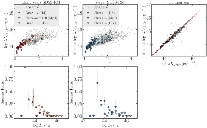
Figure 1: Comparison of the host subtracted $\lambda L_{5100}$ continuum luminosity in the gold sample of SDSS-RM quasars. The SDSS-RM parent sample is illustrated in gray, open symbols. The top left panel illustrates the gold lag measurements (colored symbols) from the first-year and four-year (early results) SDSS-RM measurements in Grier et al. (2017); Homayouni et al. (2020); Grier et al. (2019). The top middle panel shows the 7-year lag measurements in H$\beta$, Mg II, and C IV from Shen et al. (2024). The continuum luminosity here are host-subtracted using the principle component analysis as reported by Shen et al. (2015b). Overall, there is no notable difference between the luminosity in the SDSS-RM parent sample and the targets with the most reliable lag measurements in either the early SDSS-RM or 7-year lag measurements (see Table 2 for a comparison of median values in each work). The top right panel compares the first-year with the 7-year continuum luminosity in the SDSS-RM sample. Overall, the targets do not show a significant change in their luminosity. The bottom panels show the gold-lag success fraction as a function of the early-year (left) and 7-year (right) continuum luminosity. The lag success ratio exhibits a decreasing trend with increasing source luminosity. This could be due to the longer time delays of more luminous targets (e.g., Bentz et al. 2013), which may require longer observational baselines not covered by the studies in the current work.

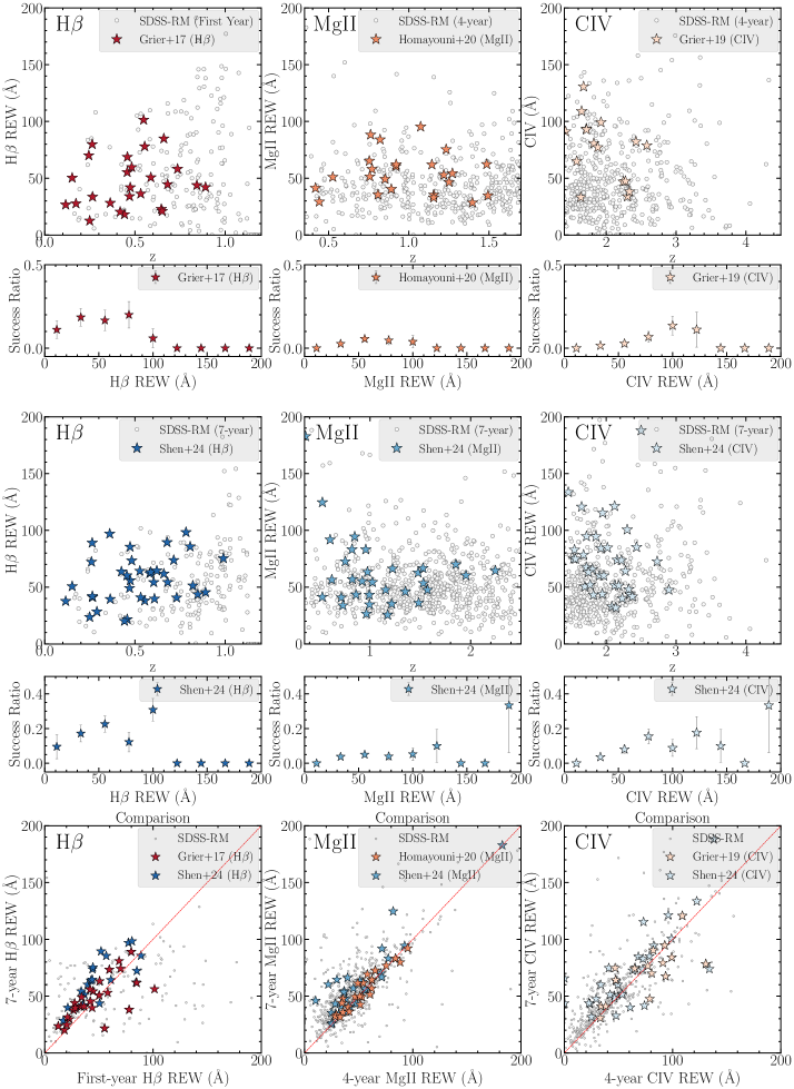
Figure 2: Comparison of the SDSS-RM REW for H$\beta$ (left column), Mg II (middle column), and C IV (right column). The gold sample in each study is identified by the colored stars and the parent sample in each case is shown with grey symbols, which reveals a uniform distribution when compared to the parent population. For each work, we also include a panel that illustrates the gold-lag success fractions as a function of REW, which reveals that there is no discernible trend evident for the success ratio and larger REW. The panels in the bottom row show the REW comparison between the early-year and the 7-year lag results. Table 2 demonstrates that gold lags in the C IV sample have marginally larger REWs compared to the other emission lines. While these larger REWs may be expected to influence the gold-lag success ratio, the observed correlation is relatively weak.

Large-scale RM surveys like the SDSS-RM program are inherently susceptible to a certain level of false-positive lag detections. Limited sampling cadence and the presence of seasonal gaps can lead to lag PDFs exhibiting well-defined peaks that satisfy our significance criteria. These peaks may arise from noisy light curves or spurious correlations within the light curve, rather than reflecting a true physical reverberation process. Therefore, Grier et al. (2017); Homayouni et al. (2020); Grier et al. (2019) and Shen et al. (2024) have employed a secondary selection process to identify the most reliable lag measurements, often referred to as the gold sample. This selection process has primarily relied on visual inspection of the light curves and lag PDFs to identify these high-confidence lag measurements. Distinguishing genuine reverberation from spurious detections remains a challenge, with the specific criteria varying between studies. Key factors for gold-lag measurement include a unimodal lag probability density function, indicating a single dominant lag value, and sufficient light curve variability. Furthermore, consistency across different analysis methods and a good fit of the applied model to the light curve data provide strong supporting evidence for the validity of the measured lag. Other approaches such as simulation-based methods and quantitative measures can provide objective assessments of lag reliability, but they often require significant computational resources, as demonstrated by Homayouni et al. (2020) and Yu et al. (2021). This is especially true for identifying a gold sample in industrial RM studies, which involves time-intensive simulations of lightcurves.

Table 1: Gold Lag Summary in SDSS-RM Survey

Targeted Emission Line	Results	$\rm N_{Sample\,Total}$	$\rm N_{Gold}$	Gold-Lag Success Ratio
H$\beta$ (first-year)	Grier et al. (2017)	222	26	12%
MgII (four-year)	Homayouni et al. (2020)	193	24	12%
CIV (four-year)	Grier et al. (2019)	349	16	5%
H$\beta$ (seven-year)	Shen et al. (2024)	186	37	20%
MgII (seven-year)	Shen et al. (2024)	714	32	4%
CIV (seven-year)	Shen et al. (2024)	494	37	7%

From the parent sample of 849 quasars in the SDSS-RM sample, the applicable redshift range for H$\beta$ lags ($0.3<z<1.14$) has limited the usable sample to 222 objects. From this subsample, Grier et al. (2017) achieved successful lag measurements for 44 quasars, with 26 classified as gold. Similarly, RM measurements of Mg II in Homayouni et al. (2020) were restricted to $0.3<z<1.7$, leading to 193 quasars in the Mg II-subsample, which yielded successful lag measurements in 57 quasars, out of which 24 were identified as gold. Grier et al. (2019) investigated C IV lags, but their analysis was limited to $1.4<z<4.5$ due to the upper redshift limit of the SDSS-RM parent sample. Out of 349 quasars, successful lag measurements were obtained for 48, only 16 of which were classified as gold. The resource-intensive nature of RM, coupled with the low yield of gold-lag measurements, motivates further investigation in the current work. Similarly for the 7-year lag results, Shen et al. (2024) recently analyzed a sample of 187 quasars for H$\beta$, 714 for Mg II, and 494 for C IV, identifying 37, 32, and 37 gold measurements, respectively. Table 1 provides a brief summary of the overall success fraction of gold-lag measurements in SDSS-RM.

4 Target Properties

We examine the extent to which inherent target properties, including both physical characteristics and statistical light-curve signatures, produce the most reliable lag measurements. To ensure that target properties do not vary significantly relative to the baseline observations, we study the properties within each study. These included one-year and four-year RM lag measurements reported by Grier et al. (2017); Homayouni et al. (2020), and Grier et al. (2019) alongside the recent seven-year results by Shen et al. (2024). This comparison aims to mitigate any significant discrepancies potentially arising from the difference in the baseline of observations (short vs. long). For each property, we also investigate the correlation between gold-lag success ratio and the property’s value. A comparative analysis of the median values for the parent and gold samples is also provided in Table 2 (physical target properties) and Table 3 (statistical light-curve properties).

Table 2: Comparative Analysis of Sample Properties: Gold and Parent

Emission Line	$\lambda L_{5100}$		REW
	log($\rm erg\,s^{-1}$)		Å
	Parent	Gold	Parent	Gold
H$\beta$ (first-year)	$44.37^{+0.37}_{-0.43}$	$44.14^{+0.24}_{-0.42}$	$44.83^{+66.95}_{-30.33}$	$42.94^{+27.09}_{-20.19}$
MgII (four-year)	$44.73^{+0.5}_{-0.41}$	$44.6^{+0.2}_{-0.29}$	$44.73^{+26.02}_{-14.9}$	$52.19^{+16.27}_{-17.09}$
CIV (four-year)	$45.09^{+0.4}_{-0.41}$	$44.86^{+0.33}_{-0.32}$	$48.0^{+43.49}_{-23.73}$	$79.77^{+17.17}_{-38.09}$
H$\beta$ (seven-year)	$44.32^{+0.42}_{-0.43}$	$44.15^{+0.31}_{-0.33}$	$54.07^{+26.83}_{-24.9}$	$54.36^{+23.4}_{-15.25}$
MgII (seven-year)	$44.75^{+0.49}_{-0.42}$	$44.65^{+0.24}_{-0.35}$	$49.3^{+23.87}_{-17.59}$	$55.83^{+27.31}_{-19.73}$
CIV (seven-year)	$45.03^{+0.39}_{-0.42}$	$44.93^{+0.37}_{-0.34}$	$47.69^{+37.29}_{-20.04}$	$67.47^{+28.65}_{-23.68}$

4.1 Continuum Luminosity

Intrinsic AGN luminosity is considered the primary driver of reverberation lag times. More luminous quasars tend to have larger time lags as observed by the $R-L$ relation (Bentz et al., 2013; Fonseca Alvarez et al., 2019), which matches basic photoionization expectations ($R_{\rm BLR}\propto\sqrt{L}$). Furthermore, luminous quasars often exhibit lower amplitude variability (MacLeod et al., 2012; Vanden Berk et al., 2004), potentially reducing the likelihood of detecting a reliable lag measurement within short observing campaigns. To explore this connection, we adopt the $\lambda L_{5100}$ luminosity as a measure of the quasar continuum luminosity. Whenever possible, we utilize directly measured $\lambda L_{5100}$ values. For sources lacking direct $\lambda L_{5100}$ measurements, we reconstruct them using $\lambda\,L_{3000}$, $\lambda\,L_{1350}$, and the bolometric corrections from Richards et al. (2006). Figure 1 illustrates the redshift and luminosity distribution of our targets. We performed a global comparison of the continuum luminosity within the gold samples of early SDSS-RM studies and the current 7-year lag measurements (Grier et al., 2017, 2019; Homayouni et al., 2020; Shen et al., 2024). This analysis did not reveal any statistically significant changes in the continuum luminosity distribution over the multi-year analysis. Additionally, we find no dependence between lag measurement success and source luminosity. The median continuum luminosity of the gold sample (in logarithmic scale) is $44.1\pm 0.1$ $\rm erg\,s^{-1}$, $44.7\pm 0.1$ $\rm erg\,s^{-1}$, and $45.0\pm 0.2$ $\rm erg\,s^{-1}$ for H$\beta$, Mg II, and C IV respectively for the early SDSS-RM lag measurements, which is similar to the median range of $44.2\pm 0.2$, $44.8\pm 0.05$, and $45.0\pm 0.1$ $\rm erg\,s^{-1}$ in the parent sample of each targeted emission line. Here the uncertaintly on the median vales are computed through bootstrap method. We find similar ranges for the gold-lag measurements in the 7-year results of Shen et al. (2024).

4.2 Rest-frame Equivalent Width

The rest-frame equivalent width (REW) of emission lines is another potential factor influencing successful lag measurement success. We investigate whether targets with larger REWs correlate with the most reliable lag measurements. For each emission line, we examine the potential relationship between its REW using PrepSpec outputs. REWs are measured from the continuum and flux provided by PrepSpec, utilizing either one-year, four-year, or seven-year average spectra. Figure 2 shows the comparisons between early-year and 7-year SDSS-RM data for the same emission lines, which reveal relatively consistent REWs over time. Furthermore, we find no direct correlation between the fraction of quasars with gold-lag measurements. Figure 2 depicts how the gold samples in each study are uniformly distributed within their respective parent samples, and the gold-lag success fraction does not reveal any specific trends with REW. While the one-year and four-year PrepSpec spectral fits did not incorporate any Fe II emission lines, the seven-year data included an Fe II template. Consequently, the 7-year measurements of Shen et al. 2024 (blue data points in Figure 2) appear to be systematically offset above the 1:1 line, suggesting that for all the three emission lines, the gold-lag estimates may be biased towards larger REWs. However, we did not observe a higher success rate for the gold-lag sample, except for C IV.

4.3 Redshift and Observed-Frame Wavelength

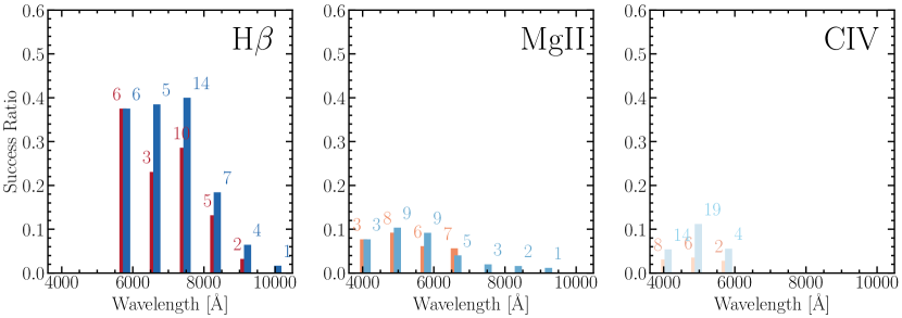
Figure 3: Lag success fraction as a function of emission-line position on the BOSS spectrograph. Early SDSS-RM measurements are depicted in reddish tones, while the 7-year lag measurements are represented by bluish tones. For H$\beta$ (left panel), we have the highest ratio of obtaining a successful lag measurement when the emission line is positioned near the center of the detector (middle thirds), and we see a significant decrease in the lag recovery rate as the H$\beta$ (left) profile falls on the edges (outer thirds) of the detector both in the single-year (Grier et al., 2017) and the 7-year (Shen et al., 2024) analyses. The effect of emission-line location on the detector in Mg II (middle) and C IV measurements (right) are more mixed; this is because the 4-year Mg II study in Homayouni et al. (2020) has been cut at $z<$1.7 due to contamination with skylines. The C IV emission line can be measured for targets at higher redshift and the lags are plausibly longer than could be recovered with the observed baseline of 4-years (Grier et al., 2019) or 7-years (Shen et al., 2024). For each wavelength bin, we also display the number of gold lags to illustrate the statistical significance in each bin.

The SDSS-RM quasars probe $0.3<z<4.5$; redshift effects limit the observable emission lines that can be targeted with RM observations and cosmological time dilation increases the observed lags. The throughput of the SDSS BOSS spectrograph exhibits a wavelength dependence across its operational range of 360 nm $<\lambda<$ 1000 nm (Smee et al., 2013). This variation is attributed to several factors, including the CCD sensitivity, the blue/red grism efficiency, the collimator characteristics, and contamination by sky lines. We next explore the potential influence of the targeted emission line’s location within the SDSS spectrograph bandpass on the gold-lag measurements. The detector edges exhibit lower sensitivity, resulting in increased noise. Therefore, we investigate whether the placement of the emission line closer to the detector center improves the probability of acquiring a successful lag measurement.

Considering the redshift range of the SDSS-RM sample (Section 2.1), prominent BLR emission lines observable include H$\beta$ at lower redshifts, Mg II in the mid-redshift range, and C IV at higher redshifts. We investigate the impact of target redshift and observed-frame wavelength for each emission line by dividing the bandpass into seven bins of equal observed wavelength range. Figure 3 compares the success ratio of the observed-frame emission line on the detector for both early-year SDSS-RM and the 7-year lag measurements. Our analysis reveals a trend of decreasing lag success with wavelength for H$\beta$, and Mg II. We also find a significantly higher success rate for the gold H$\beta$ lag measurements when the observed frame H$\beta$ is located near the mid-wavelength range of the detector. The results for C IV are less conclusive. The highest redshift in the C IV gold sample ($z$ = 2.9) restricts our ability to confirm the lag success rate beyond $\approx$6000 Å. Additionally, assessing C IV results is complicated as these targets tend to have longer rest-frame lags due to their higher luminosity and cosmological time dilation effects. Our comparison across the three emission lines suggests a clear influence only for H$\beta$ where the three central bins covering 5725 Å to 7425 Å exhibit a mean success rate of $\gtrsim$20%. The central bins from Shen et al. (2024) exhibited a higher success fraction of approximately 39% compared to the approximately 30% success rate of the central bins from Grier et al. (2017) and the neighboring bins closer to the spectrograph edges (outer thirds compared to the middle third). The results for Mg II and C IV were less definitive.

5 Light-curve Variability Characteristics

Table 3: Comparative Analysis of Light Curve Properties: Gold and Parent

Emission Line	Frac. RMS Var.		SNR2		Con. dw		Line dw
	Parent	Gold	Parent	Gold	Parent	Gold	Parent	Gold
H$\beta$ (first-year)	$0.1^{+0.24}_{-0.06}$	$0.1^{+0.14}_{-0.05}$	$10.21^{+10.08}_{-4.79}$	$13.86^{+15.68}_{-4.1}$	$0.76^{+0.56}_{-0.5}$	$0.3^{+0.5}_{-0.15}$	$1.51^{+0.4}_{-0.61}$	$0.83^{+0.6}_{-0.35}$
MgII (four-year)	$0.1^{+0.06}_{-0.04}$	$0.1^{+0.04}_{-0.03}$	$29.48^{+11.67}_{-6.7}$	$25.88^{+11.71}_{-3.48}$	$0.38^{+0.52}_{-0.24}$	$0.43^{+0.25}_{-0.33}$	$1.17^{+0.36}_{-0.43}$	$1.04^{+0.44}_{-0.5}$
CIV (four-year)	$0.11^{+0.07}_{-0.05}$	$0.14^{+0.09}_{-0.06}$	$32.96^{+18.49}_{-9.46}$	$42.34^{+15.18}_{-10.86}$	$0.53^{+0.52}_{-0.31}$	$0.4^{+0.48}_{-0.17}$	$0.96^{+0.39}_{-0.39}$	$0.54^{+0.32}_{-0.09}$
H$\beta$ (seven-year)	$0.16^{+0.25}_{-0.08}$	$0.18^{+0.14}_{-0.09}$	$23.98^{+28.77}_{-9.69}$	$51.4^{+27.15}_{-19.9}$	$0.62^{+0.43}_{-0.35}$	$0.47^{+0.39}_{-0.25}$	$1.0^{+0.52}_{-0.57}$	$0.39^{+0.38}_{-0.19}$
MgII (seven-year)	$0.1^{+0.07}_{-0.04}$	$0.1^{+0.13}_{-0.04}$	$22.33^{+14.88}_{-8.6}$	$36.3^{+14.62}_{-11.57}$	$0.67^{+0.41}_{-0.36}$	$0.38^{+0.38}_{-0.2}$	$1.39^{+0.31}_{-0.42}$	$0.78^{+0.38}_{-0.37}$
CIV (seven-year)	$0.12^{+0.08}_{-0.05}$	$0.13^{+0.06}_{-0.07}$	$33.09^{+21.39}_{-14.07}$	$46.7^{+28.63}_{-13.8}$	$0.67^{+0.42}_{-0.33}$	$0.6^{+0.37}_{-0.27}$	$1.05^{+0.38}_{-0.41}$	$0.64^{+0.37}_{-0.21}$

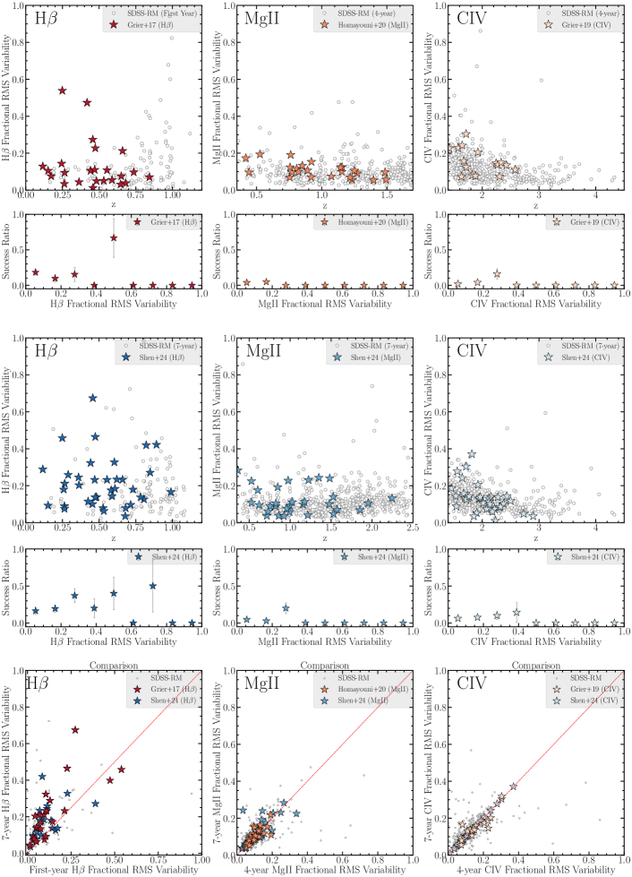
Figure 4: Fractional root-mean-square (rms) variability for H$\beta$ (left column), Mg II (middle column), and C IV (right column) as a function of redshift for early (reddish color palette) and 7-year (blueish tones) SDSS-RM results. For each work, we also include a panel that illustrate the gold-lag success fraction as a function of fractional RMS variability with similar color palettes, which reveals no trends between the gold-lag success ratio and fractional rms variability for the corresponding emission line (see Table 3 for a comparison of median values in each work). The bottom panels compare the fractional rms variability between the early-year and 7-year SDSS-RM campaigns. Our analysis reveals no statistically significant correlation between the emission line fractional rms variability and gold-lag measurements.

5.1 Fractional Variability

Quasars exhibit variability characterized by a wide range of amplitudes, wavelengths, and timescales (e.g., Collier et al., 2001; Peterson et al., 2004; Kelly et al., 2009; MacLeod et al., 2012). This variability is crucial for RM studies. However, not all quasars exhibit sufficient variability of their emission lines to enable reliable RM measurements. It is plausible that the success of lag measurements is linked to specific characteristics of the light-curve variability. Shen et al. (2024) quantified the intrinsic variability of SDSS-RM light curves using a maximum-likelihood estimator. They report the intrinsic root-mean-square (rms) variability for both the 11-year photometric light curve and the 7-year emission-line light curves. Their findings indicate that different emission lines exhibit varying degrees of intrinsic variability, although a general correlation exists between the continuum and emission-line rms variability.

We investigate the connection between emission-line rms variability and the success rate of gold-lag measurements. We utilize the fractional rms variability (normalized to the mean flux) measured by PrepSpec as described in Shen et al. (2019a). Our analysis reveals a broad distribution of fractional rms variability within the gold sample. Significant sky line residuals contaminate the H$\beta$  fractional RMS variability, potentially leading to overestimated values (Shen et al., 2019a). While the effect of skylines is less pronounced for Mg II, it is still present at $z>1.5$ among the lag measurements of Shen et al. (2024), where skylines contaminate the spectra. The Mg II lag measurements in Homayouni et al. (2020) were cut at a redshift of $z$ = 1.7 due to the contamination by skylines, therefore, there are no lag measurements for Mg II at $z>1.7$ based on the early SDSS-RM study (Homayouni et al., 2020) and the 7-year measurements reported by Shen et al. (2024) only includes three targets at z$>1.7$.

The results of this investigation are presented in Figure 4. We further compared the fractional rms variability between the early-year and 7-year studies for each emission line bottom panels in Figure 4. It is noteworthy that the 4-year and 7-year results largely follow a 1:1 trend. The deviation observed in the comparison between the 1-year and 7-year H$\beta$ fractional rms variability (bottom left corner of Figure 4) can be attributed to the variability of quasars on the observed-frame timescales. The damping timescale of quasars are longer than the seasonal monitoring duration.

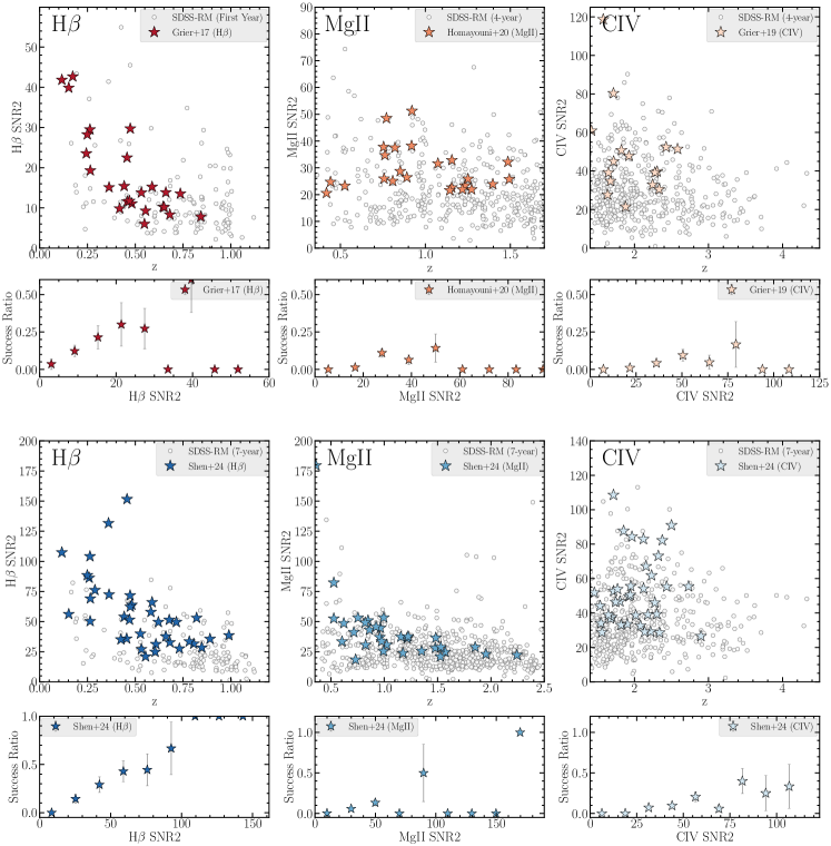
Figure 5: Emission-line variability signal-to-noise ratio (SNR2) as a function of redshift for the SDSS-RM survey. Left column shows the results for H$\beta$, middle column shows the investigation for Mg II, and the right column shows the C IV results. The early and 7-year SDSS-RM results are illustrated in reddish and blueish tones, respectively. For each work, we also include a panel that illustrates the gold-lag success fraction as a function of SNR2 with a similar color palette. Only the lag measurements by Grier et al. (2019) and Homayouni et al. (2020) adopted a SNR2 threshold for the initial target selection in lag measurements. Our analysis reveals that SNR2 has a positive trend with gold lag success fraction. This is more evident in the H$\beta$ and C IV lines, especially in the 7-year analysis compared to the earlier lag measurements. Overall, SNR2 generally exhibits a more stable indicator of gold-lag measurements when observed for multi-season campaigns. Nevertheless we find significant scatter for the SNR2 and the underlying parent sample. Table 3 provides a comparison of median SNR2 values in each work.

5.2 SNR2

Light-curve variability can also be quantified using an empirical variability metric known as the variability signal-to-noise ratio (SNR2). This metric, as computed by PrepSpec, is calculated as the square root of the chi-squared statistic ($\chi^{2}$) minus the degrees of freedom (DOF), expressed as $N$-1, where $N$ represents the number of data points in the light curve ($\rm SNR2=\sqrt{\chi^{2}-DOF}$) and the $\chi^{2}$ is calculated against the mean flux. Therefore, smaller $\rm SNR2$ indicates that the light curve is not variable compared to the mean flux and higher $\rm SNR2$ values indicate a light curve with greater intrinsic variability where the null hypothesis signifies a poor fit for a constant light curve.

To enhance the efficiency of RM lag analysis, some studies have proposed pre-selecting targets based on the variability of their emission-line light curves. This approach aims to reduce the number of unlikely candidates for lag detection. Early SDSS-RM studies, such as those by Grier et al. (2019) and Homayouni et al. (2020), employed a threshold of SNR2 $>$ 20 for their initial, larger parent samples. However, this practice was not universally adopted among the SDSS-RM work, potentially introducing bias into some early SDSS-RM results.

Both C IV and Mg II in Grier et al. (2019) and Homayouni et al. (2020) studies employed an SNR2 $>$ 20 threshold in their parent samples, whereas the lag measurements reported in Grier et al. (2017); Shen et al. (2024) did not. Notably, a strong preference for this threshold exists even though it was not consistently applied across all studies (Figure 5). While Shen et al. (2024) found a 70% lag detection rate for H$\beta$ for targets with SNR2 $>$ 35, a similar analysis of SNR2 in Grier et al. (2017) revealed that the majority of gold lags had SNR2 $<$ 20; however, this might also be connected to the higher cadence during the first-year of SDSS-RM observation (see Section 6 for a thorough discussion).

To investigate the potential relationship between SNR2 and the success of gold-lag measurements, we examined the lag measurements by Grier et al. (2017, 2019), Homayouni et al. (2020), and Shen et al. (2024). Our investigation revealed a direct correlation between SNR2 values and the gold-lag detection rate for the H$\beta$ sample compared to Mg II and C IV. While the detection rate somewhat increases with higher SNR2 for all three emission lines, the increase was more pronounced for H$\beta$. Shen et al. (2024) observed a comparable trend for all lag measurements in their dataset, regardless of whether they were classified as gold (see Figure 16 of Shen et al. (2024)). Similar to fractional RMS variability, SNR2 inherently increases with longer light-curve baselines. We therefore refrain from showing comparisons between one-year, 4-year, and 7-year analyses due to the duration and the parent sample selection criteria in Figure 5. These results indicate, although SNR2 can be a valuable preliminary screening metric, its effectiveness is influenced by the cadence and duration of monitoring.

5.3 Durbin-Watson Statistic

While our findings suggest the importance of variability as measured by SNR2, instances exist where a gold lag remains undetected despite relatively high SNR2 values. For time-series analysis software to effectively detect an RM lag, the light curve often requires a distinct “hook” or inflection feature in the continuum and line light curves. In this section, we investigate whether the presence of serial correlations in the continuum and emission line light curve would lead to a higher success in detecting a gold-lag measurement. Serial correlation refers to the dependence of current residuals (from a regression model) on past residuals, indicating a patterned behavior in the time series. A commonly used test for first-order autocorrelation, which assumes independent error terms, is the Durbin-Watson test (Durbin & Watson 1950). The Durbin–Watson test statistic is given by

$$dw=\frac{\Sigma_{t=2}^{T}(e_{t}-e_{t-1})^{2}}{\Sigma_{t=1}^{T}e_{t}^{2}}\approx 2-2r,$$ (1)

Where $e_{t}$ is the least-square residual and $r$ is the first order autocorrelation coefficient. Consequently, a value of $dw\approx 2$ indicates that the first order autocorrelation coefficient $r\approx 0$. If $dw<2$, this is an indication for positive autocorrelation $r>0$; if $dw>2$, then $r<0$. Therefore, we can assess the connection between the autocorrelation, as indicated by the $dw$ statistics, which can identify “hooks” in the light curves and might serve as a reliable predictor of the gold-lag measurements.

We illustrate the result of this comparison in Figures 6 and 7 for the continuum and emission-line light curve respectively. The dw statistic, particularly for the emission-line light curves, exhibits a strong preference for values below 1 within the gold lag sample (See Figure 7). The trend toward $dw\,<$ 1 in the gold lag sample is particularly evident in the 4-year C IV lag measurements of Grier et al. (2019) and the 7-year results reported by Shen et al. (2024). This suggests that a $dw<1$ might be an indicator for successful gold lag detection. The H$\beta$ lags of Grier et al. (2017) exhibit a less pronounced preference for $dw<1$, potentially indicating that this threshold might be more applicable for longer-term observations. Furthermore, the gold Mg II lag measurements in Homayouni et al. (2020) display a wider dw distribution, which could be related to the weaker response of the Mg II emission line to continuum variations. The continuum dw values generally exhibit a broader distribution, with most still falling below 1.5 (see Figure 6). This indicates that the $dw$ derived from the emission-line light curve is a better indicator of gold-lag measurements than $dw$ computed from the continuum light curve.

Figures 6 and 7 show the distribution of the continuum light curve dw and emission line dw in comparison to the SDSS-RM dw distribution.

Thus far, we have focused on the intrinsic properties of the quasars and their light curves, investigating how these characteristics influence the success rate of RM lag measurements. While target selection and variability are crucial aspects, another important factor in RM studies is the cadence of the observations. Given the lag measurements from the SDSS-RM observation, we now focus on the observational cadence and what are the implications for future RM campaigns.

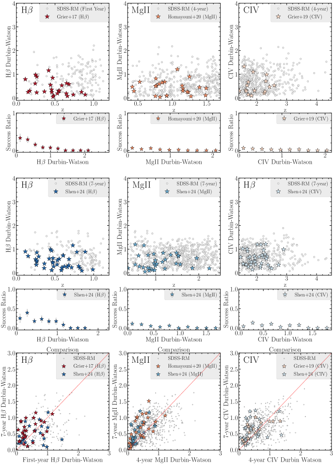
Figure 6: The Durbin-Watson statistic computed for the continuum light curves in H$\beta$, (left column), Mg II (middle column), and the C IV (right column). The gold sample in each study is identified by the colored stars and the parent sample in each case is shown with grey symbols, where the reddish color palette shows the early SDSS-RM results and blueish tones shows the 7-year results. The Durbin-Watson statistic shows the auto-correlation of the continuum light curve with a lag of one epoch. Positive serial auto-correlation ($r$ = 1) has a $dw$ = 0, no serial auto-correlation has a $dw$ = 2, and negative serial auto-correlation has a $dw$ = 4. The bottom row, compares the 7-year vs. the early-year SDSS-RM continuum Durbin-Watson statistics. We see an abundance of successful lag measurements for continuum light curves that have $dw<1$. While the gold-lag success rate does not exhibit a strong correlation with continuum light curve dw, a subtle trend may be present for H$\beta$ lags. A comparison of median dw values in Table 3 reveals that the continuum dw of gold-lag targets is generally comparable to that of the parent population.

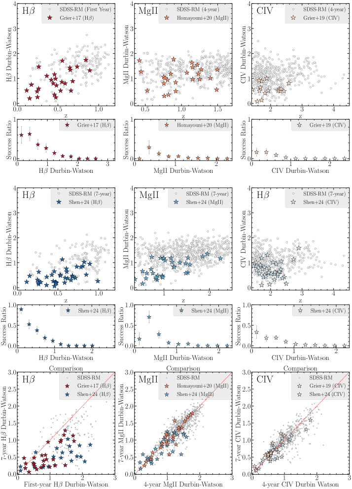
Figure 7: Similar to Figure 6 but for the H$\beta$ (left column), Mg II (middle column), and C IV (right column) light curves. Similar to Figure 6, we see that the majority of successful lag measurements correspond to light curves with $dw<$1. The gold-lag success ratio is significantly correlated with emission-line $dw$ for values less than 1. Comparative analyses indicate that the emission line $dw$ of gold-lag targets is consistently lower than for the overall population (see Table 3), with a more pronounced effect for H$\beta$ and a less significant one for Mg II.

6 Cadence Properties

6.1 Cadence Intensity in SDSS-RM

A main factor in RM observations is the cadence, as each epoch is valuable. Given the limited number of epochs available due to telescope time and weather constraints, RM programs must optimize their cadence to maximize lag measurement success. Simulations by Shen et al. (2015a) demonstrated the advantages of high-cadence observations for lag detection. While their work provided valuable guidance for the SDSS-RM initial cadence design, it had two limitations: 1) it was based on a single observation season, and 2) it used simulated light curves, which may not fully represent real-observing conditions and lag measurement success rates. To address these shortcomings, the current work examines the effect of reduced cadence using actual SDSS-RM data. This is done by comparing the impact of a relatively uniform cadence to the denser SDSS-RM cadence in the initial year (2014) and a sparser cadence in subsequent years (2015 - 2020). The SDSS-RM project, spanning seven years, employed a varying cadence design. In 2014, spectroscopy occurred every four days on average, totaling 32 epochs. From 2015 to 2017, two epochs were captured monthly, averaging 12 epochs annually. During 2018-2020, the cadence decreased to six epochs per year. Overall, the project produced a spectroscopic light curve with 90 epochs over seven years.

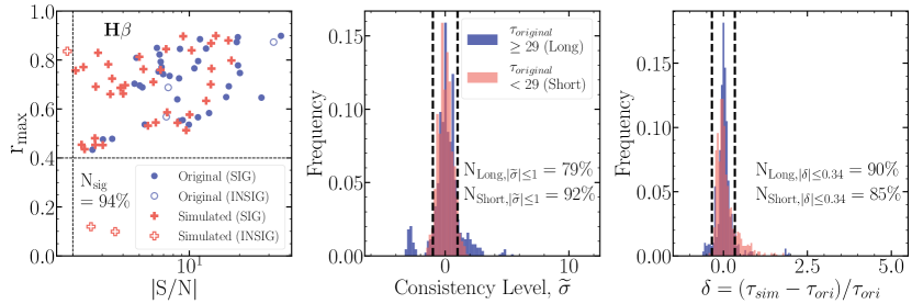
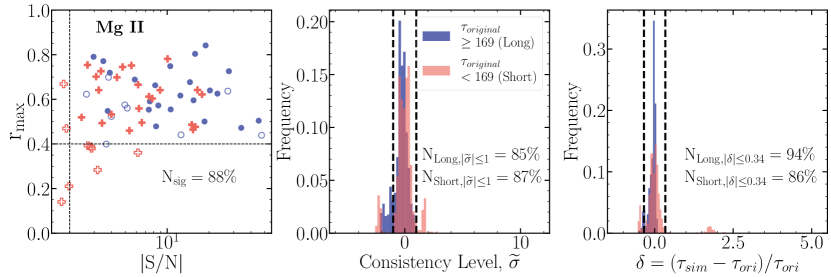
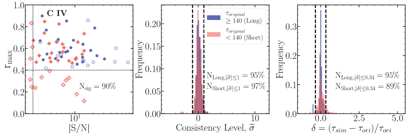
Figure 8: Summary of the simulated lag measurements from the sample of H$\beta$ (top), Mg II (middle) and C IV (bottom) from the gold results in (Shen et al., 2024). For each emission line, the panel on the left shows the maximum change in the statistical criteria in the simulated light curves. Here the dotted points represent the original statistical values on $r_{\rm max}$ and lag difference from zero, while the crosses represent the minimum statistical values among the 50 simulations for each target. The targets for which all cadence-reduced simulations are still significant are marked in blue, while the targets for which at least one cadence-reduced simulation is insignificant are marked in red. In each panel, $N_{\rm sig}$ reports the ratio of statistically significant simulations to the number of all simulations. Overall, 94% of the H$\beta$, 88% of Mg II, and 90% of the C IV simulations are still statistically significant. The middle panel illustrates the distribution of the consistency level between the original and simulated lag for long and short-lag groups (separated by the median original lag of each line). Here the dashed line identify the 1$\sigma$ consistency level. The ratio of consistent lags (to within 1$\sigma$) are reported in each panel. The right panels show the distribution of relative difference $\delta$ between the original and simulated lags divided for the short and long lag measurements. The dashed lines identify the 34% threshold of the relative difference. The ratios of lags that have a relative difference of $|\delta|\leq 0.34$ are reported for the short and long-lag samples. Overall, if we require the simulated lags are still statistically significant and consistent with original lags in $\pm 1\sigma$, we can still recover 81%, 76%, and 86% of all simulations for H$\beta$, Mg II, and for C IV respectively.

To assess the impact of reduced cadence, our experiment is to select the light curves from the gold sample of Shen et al. (2024) and decrease the epoch density for line light curves in the initial year by 40% so that the first year has $\sim$13 epochs. We maintained the same number of epochs as the actual observed in subsequent years ($\sim$13 epochs). To implement this, we first analyzed the interval distribution between epochs in 2015-2017, finding a mean of 12 days. Employing this distribution as a prior, we removed epochs at random until a subset of 13 remained. Epochs with shorter intervals, less than 12 days, were preferentially eliminated compared to those with longer cadences. This process simulated the impact of weather loss or other unforeseen events. We repeated this procedure 50 times for each target, generating 50 simulated light curves per quasar in the gold sample. This closely resembled real observations while maintaining a reduced cadence similar to that in the later years.

Finally, we run PyROA for the simulated line light curves with their original continuum light curves and apply lag identification and alias removal process to get the final lag measurement. The reason we keep the original continuum light curves and do not remove epochs from them is that the photometric observations for continuum light curves are not as expensive to make as the spectroscopic observations and are made by telescopes worldwide, so the continuum light curves are therefore densely sampled. Specifically, we have 800 epochs along 11 years and 158 epochs in 2014 (the first year of line light curves) on average, which is extremely dense with a cadence of 3 days per epoch approximately. We also perform some tests on running PyROA for cadence reduced light curves for both continuum and emission lines. The distribution of interval between one epoch to the next is almost uniform for each year, i.e., we just reduced 20% of the total epochs for continuum light curves of several targets selected randomly from the gold sample and found similar lag PDFs using PYROA Therefore, for convenience, removing epochs in the first year in the following texts refers to randomly reducing the density of epochs in the first year of the original emission line light curve to 40% unless otherwise specified.

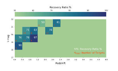
Figure 9: Overview of the lag recovery ratio binned by redshift and $i$-band magnitude. Here each bin reports the ratio of statistically significant lag measurements that are consistent to within 1$\sigma$ of the reported lag measurement in Shen et al. (2024). Overall, our light curve simulations (see Section 6.2 for detail) shows that reducing the observation cadence by $\sim$ 40% during the first year would result in slightly worse lag recovery ratios for $z<0.8$, where the H$\beta$ emission line is primary line of interest for ground-based campaigns, and often exhibits shorter lags. The result of our simulations may be conservative since they are based on the gold sample in Shen et al. (2024), which results in $\sim$ 100 in H$\beta$, Mg II, and C IV emission lines.

6.2 Impact of Reduced Cadence on Lag Success

We run all the simulated light curves through the same lag identification pipeline as Shen et al. (2024) and perform the following statistical analyses. We use three criteria to assess the difference between the original lag measurements and the simulated lag measurements for targets from the gold sample, and display the variation of simulated lags in Figure 8. The three criteria are:

• The simulated lag is still detected with the statistically significant criteria defined in Section 3: (1) less than half of the lag posterior samples are removed by our alias removal process (as defined by the $f_{peak}$ parameter in Section 3); (2) The maximum cross correlation coefficient $\rm{r_{max}}>0.4$ within $\pm 1\sigma$ of the reported PyROA lag; (3) The PyROA lag is at least $2\sigma$ different from zero lag, i.e., $\rm{|S/N|}>2$, and forPyROA, it always means that the lag is positive at $\geq 2\sigma$ significance (Shen et al., 2024);.

• The simulated lag is consistent with the original lag within $1\sigma$ uncertainties. To be more specific, we use consistency level $\tilde{\sigma}$ to quantitatively describe how well the original lag and the simulated lag are consistent within a given margin of error.

  If the simulated lag $\tau_{sim}$ is larger than the original lag $\tau_{ori}$, $\tilde{\sigma}=(\tau_{sim}-\tau_{ori})/(\sigma_{ori,upper}+\sigma_{sim,lower})>0$, where $\sigma_{ori,upper},\sigma_{sim,lower}$ is the upper uncertainties of original lag and lower uncertainties of simulated lags, respectively; on the contrary, if the simulated lag $\tau_{sim}$ is smaller than the original lag $\tau_{ori}$, $\tilde{\sigma}=(\tau_{sim}-\tau_{ori})/(\sigma_{ori,lower}+\sigma_{sim,upper})<0$, where $\sigma_{ori,lower},\sigma_{sim,upper}$ is the lower uncertainties of original lag and upper uncertainties of simulated lags, respectively.

• We determine the relative difference between the median of the 50 simulated lag $\tau_{sim}$ and the original lag $\tau_{ori}$ as $\delta=(\tau_{sim}-\tau_{ori})/\tau_{ori}$, and require the relative difference less than 34%.

The distributions of the lag selection criteria, $|\rm{S/N}|$, and $\rm{r_{max}}$ are displayed on the left panels in Figure 8. Most of the lag posterior samples given by PyROA will still have a single, prominent peak in the lower-cadence simulations, so we do not show the changes for the lag selection criteria $f_{peak}$. While the statistical values for $|\rm{S/N}|$ and $\rm{r_{max}}$ generally decreased in the lower-cadence simulations, most simulated lags still met the significance criteria. Figure 8 highlights several targets with original $|\rm{S/N}|$ and $\rm{r_{max}}$ values near the selection threshold that resulted in insignificant lag measurements under reduced cadence conditions. The simulated lags that were initially considered insignificant but later became significant are primarily found in cases with lower overall light curve quality. This suggests that the reduction in measurement quality during the first season pushed these lags below the original selection criteria. Despite having the lowest median observed-frame lag (31 days), the H$\beta$ sample still has the highest ratio of significant results. This may be attributed to the generally higher lag $|\rm{S/N}|$ and $\rm{r_{max}}$ values in the H$\beta$ sample, indicating its robustness to epoch reduction.

Our reduced-cadence simulations demonstrate that H$\beta$ lags are most resilient to a reduction in number of epochs , with 94% remaining significant after a 40% epoch reduction in the first year of SDSS-RM. For Mg II and C IV, we identified 88% and 90% of significant lags, respectively, using the criteria from Shen et al. (2024). Overall, our simulations demonstrate that we can recover $\sim$ 90% of significant results for all the three emission lines: H$\beta$, Mg II, and C IV. H$\beta$ lags exhibit the highest ratio of significant results, regardless of the original lag value. While targets with shorter original lags might be expected to be more affected by epoch reduction, we found no significant difference in the success rate for detecting long or short lags.

We display the consistency level $\tilde{\sigma}$ for significant results in the middle column of Figure 8. As described above, the $\tilde{\sigma}$ can quantitatively describe how well the original lag and the simulated lag are consistent within a given margin of error. We divided the sample into long- and short-lag groups based on their median original lags: 31 days for H$\beta$, 155 days for Mg II, and 140 days for C IV. Short-lag targets exhibited a higher degree of consistency ($|\tilde{\sigma}|<1$) compared to long-lag targets across all emission lines. The most pronounced difference was seen for H$\beta$, with short-lag targets achieving a 92% $\pm$ 1% consistency rate, surpassing the 79% $\pm$ 1% of long-lag targets. Mg II and C IV also exhibited similar trends, with short-lag targets outperforming long-lag targets by small margins. However, among the three emission lines, C IV (with the longest median original lag) demonstrated the highest overall ratio of simulations that maintained consistent results within 1$\sigma$ errors, while H$\beta$ and Mg II exhibited lower ratios. The short-lag sample may exhibit higher consistency due to its smaller absolute changes in lags and associated errors compared to the long-lag sample.

Figure 8 (right column) illustrates the distribution of relative differences between simulated and original lags for significant results of H$\beta$, Mg II, and C IV. The relative difference, $\delta$, quantifies the change in the median simulated lag relative to the original. Long-lag targets consistently exhibited a higher proportion of “similar” results ($|\delta|\leq 0.34$) compared to short-lag targets. For H$\beta$, this ratio was 90% $\pm$ 1% for long lags and 85% $\pm$ 1% for short lags. Similar trends were observed for Mg II (94% vs. 86%) and C IV (95% vs. 89%). However, if we require both statistical significance and consistency within $\pm\delta$, the lag recovery ratios are 81% for H$\beta$, 76% for Mg II, and 86% for C IV. Targets with longer original lags are slightly more susceptible to a 40% reduction in cadence during the first year ($\sim$13 epochs).

To inform future cadence design, we examined the relationship between lag recovery ratio, $i$-band magnitude, and redshift, given that SDSS-RM targets are selected based on flux limits. Figure 9 presents an overview of the lag recovery ratio binned by redshift (bin size = 0.4) and $i$-band magnitude (bin size = 1). Overall, we observed a trend of higher success ratios for brighter $i$-band magnitudes and lower redshifts. Several bins, particularly those near the boundary of the redshift-magnitude parameter space, contain fewer than five targets and may not provide statistically meaningful results. We therefore excluded these bins from Figure 9. Given our results based on seven years of observations from SDSS-RM, the limited number of significant lags detected at these redshifts and magnitudes, as also indicated by mock data in Shen et al. (2015a), underscores the challenges of measuring significant lags at these cosmological distances and magnitudes.

Our simulation results demonstrate a similar redshift and magnitude dependence for the recovery ratio as found in Shen et al. (2015a), even when comparing our 7-year observations to their 6-month mock light curves (Figures 8 and 9 in Shen et al. 2015a).

7 Summary and Implications for Future Industrial-Scale Surveys

The Sloan Digital Sky Survey Reverberation Mapping (SDSS-RM) project has offered a valuable dataset for investigating factors that influence the successful measurement of reliable RM lags in quasars. Previous SDSS-RM studies (Grier et al., 2017, 2019; Homayouni et al., 2020; Shen et al., 2024) have identified 172 high-confidence lag measurements (the gold sample). The gold lag success rate in SDSS-RM varies between 4% and 20% depending on the emission line type and survey length (see Table 1). To better understand the gold-lag success rate, and analysis turnaround, we have analyzed the impact of intrinsic target properties, light-curve statistics, observation cadence, and the number of observing epochs on lag measurement. Our goal is to enhance the efficiency of lag analysis by identifying targets and light curves with a higher probability of success. This will facilitate a more strategic approach, allowing for efficient prioritization of targets and ultimately maximizing the scientific return of surveys that are similar to SDSS-RM.

For each individual lag study, we examined the correlation between target properties (luminosity, equivalent width of the targeted emission line, and redshift) and light curve characteristics (fractional RMS variability, SNR2, and Durbin-Watson statistics) with the success of measuring gold lags. Comparison of the target properties such as luminosity $\lambda L_{5100}$ (Figure 1) and emission line equivalent width (Figure 2) does not reveal a correlation with the gold-lag measurements. We observed a significantly higher success rate ($\gtrsim$20%) in detecting gold lags when the H$\beta$ line is positioned near the center of the observed-frame spectroscopic range. However, the impact of emission line position on detection is less strong for Mg II due to redshift cuts and for C IV due to potentially longer lags exceeding our baseline coverage (Figure 4).

As for the light curve characteristic, while fractional RMS variability shows no correlation with successful lag measurement, the empirical variability metric SNR2 exhibits a positive trend. The H$\beta$ SNR2 in the gold sample of Grier et al. (2017) and Shen et al. (2024) is significantly higher for the gold lags than those of the parent sample. This is aligned with Shen et al. (2024)’s observations on the role of variability metrics as measured by SNR2 for general lag detection. Similarly, the gold lags measured by Grier et al. (2019) and Homayouni et al. (2020) maybe inconclusive for the impact of SNR2 as their initial samples were restricted to only have SNR2$>20$.

The Durbin-Watson ($dw$) statistic is a reliable indicator of gold-lag measurements, particularly when applied to emission line light curves. While the $dw$ statistic for the continuum light curve shows a weaker correlation, analyzing the emission line $dw$ reveals a stronger trend. For Mg II, the $dw$ statistic exhibits a weaker correlation with gold lag success compared to H$\beta$ and C IV. This is likely due to Mg II’s lower variability amplitude (Sun et al., 2015). Overall, our analysis suggests that the $dw$ statistic, especially when applied to emission line light curves, is a valuable tool for efficiently filtering targets and predicting the likelihood of obtaining reliable lag measurements, particularly in large datasets.

Additionally, we investigate the impact of reducing the SDSS-RM cadence on lag measurements based on the observed quasar light curves of Shen et al. (2024). We simulate multi-year light curves with 40% reduction in cadence during the first year and compare with the existing lag measurements for the same target. While most statistically significant lags are preserved after cadence removal ($\sim$90% or higher for all emission lines studied: H$\beta$, Mg II, and C IV), a small percentage become insignificant. The consistency between original and simulated lags (within a margin of error) is generally higher for shorter lags compared to longer lags. However, when we consider the lag similarity, it is worse for shorter lags. This is likely due to the decreased temporal resolution, which can limit the ability to capture the rapid variations associated with shorter lags. Furthermore, we find that the recovery rate is slightly lower for fainter or higher redshift quasars (Figure 9). These results are consistent with earlier studies using shorter mock light curves Shen et al. (2015a). Overall, our simulations indicate that a mixed cadence strategy, featuring a period of higher cadence followed by lower cadence as in SDSS-RM, provides only a marginal improvement in gold-lag measurement compared to a more uniform cadence, which can still recover 90% of the lags.

References

- Bao et al. (2022) Bao, D.-W., Brotherton, M. S., Du, P., et al. 2022, arXiv e-prints, arXiv:2207.00297. https://arxiv.org/abs/2207.00297
- Barth et al. (2011) Barth, A. J., Nguyen, M. L., Malkan, M. A., et al. 2011, ApJ, 732, 121, doi: 10.1088/0004-637X/732/2/121
- Barth et al. (2015) Barth, A. J., Bennert, V. N., Canalizo, G., et al. 2015, ApJS, 217, 26, doi: 10.1088/0067-0049/217/2/26
- Bellm et al. (2019) Bellm, E. C., Kulkarni, S. R., Graham, M. J., et al. 2019, PASP, 131, 018002, doi: 10.1088/1538-3873/aaecbe
- Bentz & Katz (2015) Bentz, M. C., & Katz, S. 2015, Publications of the Astronomical Society of the Pacific, 127, 67, doi: 10.1086/679601
- Bentz et al. (2021) Bentz, M. C., Williams, P. R., Street, R., et al. 2021, ApJ, 920, 112, doi: 10.3847/1538-4357/ac19af
- Bentz et al. (2008) Bentz, M. C., Walsh, J. L., Barth, A. J., et al. 2008, ApJ, 689, L21, doi: 10.1086/595719
- Bentz et al. (2009) —. 2009, ApJ, 705, 199, doi: 10.1088/0004-637X/705/1/199
- Bentz et al. (2010) Bentz, M. C., Horne, K., Barth, A. J., et al. 2010, ApJ, 720, L46, doi: 10.1088/2041-8205/720/1/L46
- Bentz et al. (2013) Bentz, M. C., Denney, K. D., Grier, C. J., et al. 2013, ApJ, 767, 149, doi: 10.1088/0004-637X/767/2/149
- Blandford & McKee (1982) Blandford, R. D., & McKee, C. F. 1982, ApJ, 255, 419, doi: 10.1086/159843
- Blanton et al. (2017) Blanton, M. R., Bershady, M. A., Abolfathi, B., et al. 2017, AJ, 154, 28, doi: 10.3847/1538-3881/aa7567
- Cackett et al. (2021) Cackett, E. M., Bentz, M. C., & Kara, E. 2021, iScience, 24, 102557, doi: 10.1016/j.isci.2021.102557
- Clavel et al. (1991) Clavel, J., Reichert, G. A., Alloin, D., et al. 1991, ApJ, 366, 64, doi: 10.1086/169540
- Collier et al. (2001) Collier, S., Crenshaw, D. M., Peterson, B. M., et al. 2001, ApJ, 561, 146, doi: 10.1086/323234
- Collier et al. (1998) Collier, S. J., Horne, K., Kaspi, S., et al. 1998, ApJ, 500, 162, doi: 10.1086/305720
- Dalla Bontà et al. (2020) Dalla Bontà, E., Peterson, B. M., Bentz, M. C., et al. 2020, ApJ, 903, 112, doi: 10.3847/1538-4357/abbc1c
- de Jong et al. (2019) de Jong, R. S., Agertz, O., Berbel, A. A., et al. 2019, The Messenger, 175, 3, doi: 10.18727/0722-6691/5117
- De Rosa et al. (2015) De Rosa, G., Peterson, B. M., Ely, J., et al. 2015, ApJ, 806, 128, doi: 10.1088/0004-637X/806/1/128
- Denney et al. (2016a) Denney, K. D., Horne, K., Brandt, W. N., et al. 2016a, ApJ, 833, 33, doi: 10.3847/1538-4357/833/1/33
- Denney et al. (2010) Denney, K. D., Peterson, B. M., Pogge, R. W., et al. 2010, ApJ, 721, 715, doi: 10.1088/0004-637X/721/1/715
- Denney et al. (2016b) Denney, K. D., Horne, K., Shen, Y., et al. 2016b, ApJS, 224, 14, doi: 10.3847/0067-0049/224/2/14
- Dexter et al. (2019) Dexter, J., Xin, S., Shen, Y., et al. 2019, arXiv e-prints, arXiv:1906.10138. https://arxiv.org/abs/1906.10138
- Donnan et al. (2021) Donnan, F. R., Horne, K., & Hernández Santisteban, J. V. 2021, MNRAS, 508, 5449, doi: 10.1093/mnras/stab2832
- Du et al. (2014) Du, P., Hu, C., Lu, K.-X., et al. 2014, ApJ, 782, 45, doi: 10.1088/0004-637X/782/1/45
- Du et al. (2016a) Du, P., Lu, K.-X., Zhang, Z.-X., et al. 2016a, ApJ, 825, 126, doi: 10.3847/0004-637X/825/2/126
- Du et al. (2016b) Du, P., Lu, K.-X., Hu, C., et al. 2016b, ApJ, 820, 27, doi: 10.3847/0004-637X/820/1/27
- Eisenstein et al. (2011) Eisenstein, D. J., Weinberg, D. H., Agol, E., et al. 2011, AJ, 142, 72, doi: 10.1088/0004-6256/142/3/72
- Fonseca Alvarez et al. (2019) Fonseca Alvarez, G., Trump, J. R., Homayouni, Y., et al. 2019, arXiv e-prints, arXiv:1910.10719. https://arxiv.org/abs/1910.10719
- Fries et al. (2023) Fries, L. B., Trump, J. R., Davis, M. C., et al. 2023, ApJ, 948, 5, doi: 10.3847/1538-4357/acbfb7
- Fukugita et al. (1996) Fukugita, M., Ichikawa, T., Gunn, J. E., et al. 1996, AJ, 111, 1748, doi: 10.1086/117915
- Gaskell & Peterson (1987) Gaskell, C. M., & Peterson, B. M. 1987, ApJS, 65, 1, doi: 10.1086/191216
- Gaskell & Sparke (1986) Gaskell, C. M., & Sparke, L. S. 1986, ApJ, 305, 175, doi: 10.1086/164238
- GRAVITY Collaboration et al. (2018) GRAVITY Collaboration, Sturm, E., Dexter, J., et al. 2018, Nature, 563, 657, doi: 10.1038/s41586-018-0731-9
- GRAVITY Collaboration et al. (2020) GRAVITY Collaboration, Amorim, A., Bauböck, M., et al. 2020, A&A, 643, A154, doi: 10.1051/0004-6361/202039067
- GRAVITY Collaboration et al. (2021) GRAVITY Collaboration, et al. 2021, A&A, 648, A117, doi: 10.1051/0004-6361/202040061
- GRAVITY Collaboration et al. (2024) GRAVITY Collaboration, Amorim, A., Bourdarot, G., et al. 2024, arXiv e-prints, arXiv:2401.07676, doi: 10.48550/arXiv.2401.07676
- Grier et al. (2012) Grier, C. J., Peterson, B. M., Pogge, R. W., et al. 2012, ApJ, 755, 60, doi: 10.1088/0004-637X/755/1/60
- Grier et al. (2013) Grier, C. J., Peterson, B. M., Horne, K., et al. 2013, ApJ, 764, 47, doi: 10.1088/0004-637X/764/1/47
- Grier et al. (2016) Grier, C. J., Brandt, W. N., Hall, P. B., et al. 2016, ApJ, 824, 130, doi: 10.3847/0004-637X/824/2/130
- Grier et al. (2017) Grier, C. J., Trump, J. R., Shen, Y., et al. 2017, ApJ, 851, 21, doi: 10.3847/1538-4357/aa98dc
- Grier et al. (2019) Grier, C. J., Shen, Y., Horne, K., et al. 2019, ApJ, 887, 38, doi: 10.3847/1538-4357/ab4ea5
- Gunn et al. (2006) Gunn, J. E., Siegmund, W. A., Mannery, E. J., et al. 2006, AJ, 131, 2332, doi: 10.1086/500975
- Hemler et al. (2019) Hemler, Z. S., Grier, C. J., Brandt, W. N., et al. 2019, ApJ, 872, 21, doi: 10.3847/1538-4357/aaf1bf
- Homayouni et al. (2019) Homayouni, Y., Trump, J. R., Grier, C. J., et al. 2019, ApJ, 880, 126, doi: 10.3847/1538-4357/ab2638
- Homayouni et al. (2020) —. 2020, ApJ, 901, 55, doi: 10.3847/1538-4357/ababa9
- Homayouni et al. (2023) Homayouni, Y., De Rosa, G., Plesha, R., et al. 2023, ApJ, 948, 85, doi: 10.3847/1538-4357/acc45a
- Horne et al. (2021) Horne, K., De Rosa, G., Peterson, B. M., et al. 2021, ApJ, 907, 76, doi: 10.3847/1538-4357/abce60
- Hu et al. (2015) Hu, C., Du, P., Lu, K.-X., et al. 2015, ApJ, 804, 138, doi: 10.1088/0004-637X/804/2/138
- Ivezić et al. (2019) Ivezić, Ž., Kahn, S. M., Tyson, J. A., et al. 2019, ApJ, 873, 111, doi: 10.3847/1538-4357/ab042c
- Kaiser et al. (2010) Kaiser, N., Burgett, W., Chambers, K., et al. 2010, in Society of Photo-Optical Instrumentation Engineers (SPIE) Conference Series, Vol. 7733, Ground-based and Airborne Telescopes III, ed. L. M. Stepp, R. Gilmozzi, & H. J. Hall, 77330E, doi: 10.1117/12.859188
- Kaspi et al. (2007) Kaspi, S., Brandt, W. N., Maoz, D., et al. 2007, ApJ, 659, 997, doi: 10.1086/512094
- Kaspi et al. (2000) Kaspi, S., Smith, P. S., Netzer, H., et al. 2000, ApJ, 533, 631, doi: 10.1086/308704
- Kelly et al. (2009) Kelly, B. C., Bechtold, J., & Siemiginowska, A. 2009, ApJ, 698, 895, doi: 10.1088/0004-637X/698/1/895
- Kinemuchi et al. (2020) Kinemuchi, K., Hall, P. B., McGreer, I., et al. 2020, ApJS, 250, 10, doi: 10.3847/1538-4365/aba43f
- King et al. (2015) King, A. L., Martini, P., Davis, T. M., et al. 2015, MNRAS, 453, 1701, doi: 10.1093/mnras/stv1718
- Kormendy & Ho (2013) Kormendy, J., & Ho, L. C. 2013, arXiv e-prints, arXiv:1308.6483. https://arxiv.org/abs/1308.6483
- Li et al. (2019) Li, J., Shen, Y., Brandt, W. N., et al. 2019, ApJ, 884, 119, doi: 10.3847/1538-4357/ab41fb
- Li et al. (2021) Li, J. I. H., Shen, Y., Ho, L. C., et al. 2021, ApJ, 906, 103, doi: 10.3847/1538-4357/abc8e6
- Li et al. (2023) —. 2023, ApJ, 954, 173, doi: 10.3847/1538-4357/acddda
- Li et al. (2014) Li, Y.-R., Wang, J.-M., Hu, C., Du, P., & Bai, J.-M. 2014, ApJ, 786, L6, doi: 10.1088/2041-8205/786/1/L6
- Lira et al. (2018) Lira, P., Kaspi, S., Netzer, H., et al. 2018, ApJ, 865, 56, doi: 10.3847/1538-4357/aada45
- MacLeod et al. (2010) MacLeod, C. L., Ivezić, Ž., Kochanek, C. S., et al. 2010, ApJ, 721, 1014, doi: 10.1088/0004-637X/721/2/1014
- MacLeod et al. (2012) MacLeod, C. L., Ivezić, Ž., Sesar, B., et al. 2012, ApJ, 753, 106, doi: 10.1088/0004-637X/753/2/106
- Penton et al. (2022) Penton, A., Malik, U., Davis, T. M., et al. 2022, MNRAS, 509, 4008, doi: 10.1093/mnras/stab3027
- Peterson (1993) Peterson, B. M. 1993, Publications of the Astronomical Society of the Pacific, 105, 247, doi: 10.1086/133140
- Peterson et al. (2004) Peterson, B. M., Ferrarese, L., Gilbert, K. M., et al. 2004, ApJ, 613, 682, doi: 10.1086/423269
- Richards et al. (2006) Richards, G. T., Lacy, M., Storrie-Lombardi, L. J., et al. 2006, ApJS, 166, 470, doi: 10.1086/506525
- Shen et al. (2015a) Shen, Y., Brandt, W. N., Dawson, K. S., et al. 2015a, The Astrophysical Journal Supplement Series, 216, 4, doi: 10.1088/0067-0049/216/1/4
- Shen et al. (2015b) Shen, Y., Greene, J. E., Ho, L. C., et al. 2015b, The Astrophysical Journal, 805, 96, doi: 10.1088/0004-637X/805/2/96
- Shen et al. (2016) Shen, Y., Horne, K., Grier, C. J., et al. 2016, ApJ, 818, 30, doi: 10.3847/0004-637X/818/1/30
- Shen et al. (2019a) Shen, Y., Hall, P. B., Horne, K., et al. 2019a, ApJS, 241, 34, doi: 10.3847/1538-4365/ab074f
- Shen et al. (2019b) Shen, Y., Grier, C. J., Horne, K., et al. 2019b, ApJ, 883, L14, doi: 10.3847/2041-8213/ab3e0f
- Shen et al. (2024) —. 2024, arXiv e-prints, arXiv:2305.01014, doi: 10.48550/arXiv.2305.01014
- Smee et al. (2013) Smee, S. A., Gunn, J. E., Uomoto, A., et al. 2013, AJ, 146, 32, doi: 10.1088/0004-6256/146/2/32
- Starkey et al. (2016) Starkey, D. A., Horne, K., & Villforth, C. 2016, MNRAS, 456, 1960, doi: 10.1093/mnras/stv2744
- Sun et al. (2015) Sun, M., Trump, J. R., Shen, Y., et al. 2015, ApJ, 811, 42, doi: 10.1088/0004-637X/811/1/42
- Swann et al. (2019) Swann, E., Sullivan, M., Carrick, J., et al. 2019, The Messenger, 175, 58, doi: 10.18727/0722-6691/5129
- U et al. (2022) U, V., Barth, A. J., Vogler, H. A., et al. 2022, ApJ, 925, 52, doi: 10.3847/1538-4357/ac3d26
- Vanden Berk et al. (2004) Vanden Berk, D. E., Wilhite, B. C., Kron, R. G., et al. 2004, ApJ, 601, 692, doi: 10.1086/380563
- Wanders et al. (1997) Wanders, I., Peterson, B. M., Alloin, D., et al. 1997, The Astrophysical Journal Supplement Series, 113, 69, doi: 10.1086/313054
- Wang et al. (2019) Wang, S., Shen, Y., Jiang, L., et al. 2019, ApJ, 882, 4, doi: 10.3847/1538-4357/ab322b
- Yu et al. (2020) Yu, Z., Kochanek, C. S., Peterson, B. M., et al. 2020, MNRAS, 491, 6045, doi: 10.1093/mnras/stz3464
- Yu et al. (2021) Yu, Z., Martini, P., Penton, A., et al. 2021, MNRAS, 507, 3771, doi: 10.1093/mnras/stab2244
- Zastrocky et al. (2024) Zastrocky, T. E., Brotherton, M. S., Du, P., et al. 2024, arXiv e-prints, arXiv:2404.07343, doi: 10.48550/arXiv.2404.07343
- Zu et al. (2011) Zu, Y., Kochanek, C. S., & Peterson, B. M. 2011, ApJ, 735, 80, doi: 10.1088/0004-637X/735/2/80