On the equivalence of Prony and Lanczos methods for Euclidean correlation functions

Abstract

We investigate the oblique Lanczos method recently put forward in Ref. Wagman:2024rid (1) for analysing Euclidean correlators in lattice field theories and show that it is analytically equivalent to the well known Prony Generalised Eigenvalue Method (PGEVM). Moreover, we discuss that the signal-to-noise problem is not alleviated by either of these two methods. Still, both methods show clear advantages when compared to the standard effective mass approach.

1 Introduction

In lattice field theory, Euclidean two-point correlation functions $C$ represent the central objects to be determined numerically in Monte Carlo simulations. They are estimated from vacuum expectation values of local operators $O_{i},O_{j}$ with appropriate quantum numbers

$$C_{ij}(t-t^{\prime})\ =\ \langle\,O_{i}^{\dagger}(t)\ O_{j}(t^{\prime})\,\rangle\,.$$ (1)

They allow one to access energy eigenvalues of the lattice Hamiltonian and operator matrix elements via the spectral decomposition for energy levels $0<E_{1}<E_{2}<\ldots$ for instance for a single operator $O$

$$C(t)\ =\ \sum_{n}|\langle 0|O|n\rangle|^{2}e^{-E_{n}t}\,.$$ (2)

The ground state energy level can then be determined from $C(t)$ at sufficiently large $t$.

Since typically $C(t)$ is being determined in stochastic Monte Carlo simulations, also the statistical uncertainty needs to be estimated from the corresponding variance. As discussed by Lepage in Ref. Lepage:1989 (2), the variance can be understood as a correlation function itself decaying exponentially with a potentially smaller energy level $E_{1}^{\prime}$, leading to the infamous signal-to-noise (StN) problem

$$\operatorname{StN}(t)\ \propto\ e^{-\Delta E\,t},$$ (3)

with $\Delta E=E_{1}-E_{1}^{\prime}/2$. The most famous example is probably the nucleon two-point function, which decays at large $t$ proportional to $\exp(-M_{N}t)$, and the variance with $\exp(-3M_{\pi}t)$. Therefore, the StN ratio for the nucleon is decreasing exponentially with $\exp(-(M_{N}-3M_{\pi}/2)t)$. The most famous exception from this StN problem is the pion two-point function, which can be shown to have a constant StN ratio at large $t$-values.

This StN problem triggered a lot of effort to find novel methods which either allow to determine energy levels at earlier Euclidean times, or to tame the increasing StN ratio. One widely used method in the former class is the Generalised Eigenvalue Method (GEVM) Michael:1982gb (3, 4, 5), which however requires a correlator matrix $C_{ij}(t)$. The Prony GEVM (PGEVM) Fischer:2020bgv (6) (see Ref. Prony:1795 (7) for the original paper) or generalised pencil of function method, on the other hand, can be used with single correlation functions and allows to work at earlier times, too. For a method based on ordinary differential equations see Ref. Romiti:2019qim (8).

Recently, the author of Ref. Wagman:2024rid (1) applied the Lanczos method to this problem. Wagman argues in the paper that the Lanczos method does both, allow extraction of energy levels at early $t$-values and to tame the StN problem at late $t$-values.

In this paper we show that Lanczos is equivalent to the PGEVM, also on noisy data. Moreover, we cannot confirm that the StN problem is alleviated by either of the methods. Still, both Lanczos and PGEVM appear to be very useful in controlling systematic effects.

2 Methods

The simplest way to analyse Euclidean correlation functions is via the $\log$-effective mass

$$M_{\mathrm{eff}}(t)\ =\ -\log\left(\frac{C(t+1)}{C(t)}\right)\,,$$ (4)

applicable to correlation functions without back-propagating states. For correlators periodic in time taking the $\log$ is not sufficient, which is why one numerically inverts $f_{t}(M)=\cosh(M(t+1))/\cosh(Mt)$ for $M$ to define

$$\hat{M}_{\mathrm{eff}}(t)=[f_{t}(M)]^{-1}\,.$$ (5)

2.1 Oblique Lanczos

The oblique Lanczos method is well known and was applied to correlation functions $C(t)$ Eq. 1 for the first time by Wagman in Ref. Wagman:2024rid (1). The algorithm we have implemented is summarised in listing 1. To our understanding this is the algorithm the author has used to obtain the results presented in Ref. Wagman:2024rid (1). Note that we refer here to the original version of Ref. Wagman:2024rid (1) posted to the arXiv. For the application of Lanczos to the estimation of matrix elements see Ref. Hackett:2024xnx (9).

The Lanczos method produces sets of bi-orthogonal vectors $|v_{i}\rangle$ and $|w_{j}\rangle$ which are used to construct at iteration step $n$ the tri-diagonal matrix

$$T_{n}\ =\ W_{n}^{t}TV_{n}^{~{}}\,.$$ (6)

Note that in contrast to Ref. Wagman:2024rid (1) we use $n$ as the iteration count instead of $m$. The elements of $T_{n}$ can be computed from $2n$ elements of the correlation function $C(0),C(1),C(2),\ldots$ without the need to explicitly construct the $|v_{i}\rangle$ and $|w_{j}\rangle$.

The eigenvalues $\{\lambda_{i}\}$ of $T_{n}$ are equal to the eigenvalues of $T$ if the rank of $T$ is $n$. For rank of $T$ larger than $n$ the eigenvalues of $T_{n}$ approximate the eigenvalues of $T$. For details on the convergence see Ref. Wagman:2024rid (1) or the mathematical literature. The eigenvalues $\lambda_{i}$ are related to the ground state energy via

$$E_{n}=-\log(\lambda_{\mathrm{max}})$$

with $\lambda_{\mathrm{max}}$ the largest real eigenvalue smaller than 1.

Algorithm 1 Oblique Lanczos for LFT

1:Input: Correlator $C(t)$ for $t=0,...,2N-1$.

2:for $n=1,\ldots,N$ do

3:     set $A_{1}^{k}=C(k)/C(0)\,,\quad k>0$

4:     $\alpha_{1}=A_{1}^{1}\,,\ \beta_{1}=\gamma_{1}=0$

5:     $B_{1}^{k}=G_{1}^{k}=0$

6:     for $j=1,\ldots,n-1$ do

7:         use eq. (53) Ref. Wagman:2024rid (1)

$$\langle s_{j+1}|r_{j+1}\rangle=A_{j}^{2}-\alpha_{j}^{2}-\beta_{j}\gamma_{j}$$

8:         use eq (41) Ref. Wagman:2024rid (1)

$$\rho_{j+1}=\sqrt{|\langle s_{j+1}|r_{j+1}\rangle|}\,,\quad\tau_{j+1}=\frac{\langle s_{j+1}|r_{j+1}\rangle}{\rho_{j+1}}$$

9:         Set $k_{\mathrm{max}}=2(n-j)+1$

10:         for $k=2,\ldots,k_{\mathrm{max}}$ do

11:              Use eqs.(44) and (45) Ref. Wagman:2024rid (1)

$$\begin{split}G_{j+1}^{k}&=\frac{1}{\tau_{j+1}}\left(A_{j}^{k+1}-\alpha_{j}A_{j}^{k}-\gamma_{j}B_{j}^{k}\right)\\ B_{j+1}^{k}&=\frac{1}{\rho_{j+1}}\left(A_{j}^{k+1}-\alpha_{j}A_{j}^{k}-\beta_{j}G_{j}^{k}\right)\\ \end{split}$$

12:         end for

13:         for $k=2,\ldots,k_{\mathrm{max}}$ do

14:              Use eq.(46) Ref. Wagman:2024rid (1) and note that $A_{0}^{k}$ is not needed, because $\gamma_{1}=\beta_{1}=0$

$$\begin{split}A_{j+1}^{k}=&\frac{1}{\tau_{j+1}\rho_{j+1}}\left(A_{j}^{k+2}-2\alpha_{j}A_{j}^{k+1}\right.\\ &+\alpha_{j}^{2}A_{j}^{k}+\alpha_{j}(\beta_{j}G_{j}^{k}+\gamma_{j}B_{j}^{k})\\ &\left.-(\beta_{j}G_{j}^{k+1}+\gamma_{j}G_{j}^{k+1})+\gamma_{j}\beta_{j}A_{j-1}^{k}\right)\\ \end{split}$$

15:         end for

16:         Set

$$\alpha_{j+1}=A_{j+1}^{1}\,,\gamma_{j+1}=G_{j+1}^{1}\,,\beta_{j+1}=B_{j+1}^{1}$$

17:     end for

18:     Diagonalise the tri-diagonal matrix eq.(48) Ref. Wagman:2024rid (1) and obtain eigenvalues $\{\lambda_{i}\}$

19:     Reduce to the set $\{\lambda_{i}:\,0<\lambda_{i}<1\,,\ \operatorname{Im}(\lambda_{i})=0\}$

20:     Set $E_{n}=-\log(\lambda_{\mathrm{max}})$

21:end for

2.2 Prony GEVM

The second method we consider is the PGEVM Fischer:2020bgv (6), which is a variant of the Prony method Prony:1795 (7), see also Refs. Fleming:2004hs (10, 11, 12, 13, 14). It is equivalent to the so-called generalised pencil of function method (GPOF). For matrix elements there is a discussion in Ref. Ottnad:2017mzd (15). For the PGEVM first a $n\times n$ symmetric Hankel matrix

$$H_{ij}(t)=C(t+i\Delta+j\Delta)\,,\ 0\leq i,j<n\,,$$ (7)

is constructed from the correlation function $C(t)$ for each $t$ with $\Delta>0$ an additional parameter. Note that $H$ is symmetric, but for noisy data not necessarily positive definite. Next, the following GEVP

$$H(t+\delta t)\cdot v_{l}(t)\ =\ \Lambda_{l}^{n}(t,\delta t)H(t)\cdot v_{l}(t)$$ (8)

is solved for eigenvalues $\Lambda_{l}^{n}$ and eigenvectors $v_{l}$, with another constant parameter $\delta t\geq 1$. The $\Lambda_{l}^{n}$ can be shown to have the form

$$\Lambda_{l}^{n}(t,\delta t)\ =\ e^{-E_{l}\delta t}$$ (9)

independent of $t$ if $n$ is large enough to resolve all relevant states contributing to $C(t)$, see Ref. Fischer:2020bgv (6) and references therein. For convenience, we then define

$$\tilde{M}_{n}(t)\ =\ -\frac{\log\left(\Lambda_{0}^{n}(t,\delta t)\right)}{\delta t}\,.$$ (10)

In practice one often chooses $\delta t$ odd and $\Delta$ even, such that $H(t)$ and $H(t+\delta t)$ contain disjoint elements of $C(t)$.

The method analogous to Lanczos discussed above is to change $n=1,\ldots,n_{\mathrm{max}}$ for $\delta t$ and $\Delta$ fixed. The corresponding algorithm we implemented is summarised in listing 2.

Algorithm 2 PGEVM for LFT

1:Input: $t_{0}$, $\delta t$, $n_{\text{max}}$, and Correlator $C(t)$ for $t=0,...,T-1$

2:for $n=1,\ldots,n_{\mathrm{max}}$ do

3:     construct $H(t_{0}+\delta t)$ and $H(t_{0})$

4:     determine $\{\Lambda_{l}^{n}\}$ from

$$H(t_{0}+\delta t)\cdot v_{l}(t_{0})\ =\ \Lambda_{l}^{n}(t_{0},\delta t)H(t_{0})\cdot v_{l}(t_{0})$$

5:     Reduce to the set $\{\Lambda_{l}^{n}:\,0<\Lambda_{l}^{n}<1\,,\ \operatorname{Im}(\Lambda_{l}^{n})=0\}$

6:     Set $\tilde{M}_{n}(t)=-\log(\Lambda_{\mathrm{max}}^{n})/\delta t$

7:end for

2.3 Relation between Lanczos and PGEVM

Let us first consider the PGEVM. The Hankel matrix $H(t)$ Eq. 7 of size $n\times n$ contains the $2n-1$ correlator elements $C(t),C(t+\Delta),\ldots,C(t+2(n-1)\Delta)$. An identical number of correlator elements enters $H(t+\delta t)$. However, depending on the values of $\Delta$ and $\delta t$, there can be significant overlap in the correlator elements entering $H(t)$ and $H(t+\delta t)$.

If one chooses $\Delta=1$ and $\delta t=1$, there are $2n$ correlator elements entering in total, namely $C(t_{0}),C(t_{0}+1),\ldots,C(t_{0}+2n-1)$. Thus, choosing $t_{0}=0$, $\Delta=1$ and $\delta t=1$ the PGEVM is based on the same correlator input like the oblique Lanczos for the same $n$. In fact, PGEVM and Lanczos are exactly equivalent and, therefore, expected to yield identical results. The argument is as follows: following the notation of Ref. Wagman:2024rid (1), the correlator Eq. 1 for $O_{i}=O_{j}=O$ reads

$$C(i)=\langle\psi|T^{i}|\psi\rangle\,,$$ (11)

with $T=\exp(-\mathcal{H}a)$ the Euclidean time evolution operator, $a$ the lattice spacing, and $\mathcal{H}$ the lattice Hamiltonian. Now, both methods compute the projection of $T$ on the space spanned by the vectors

$$|\varphi_{0}\rangle,\,|\varphi_{1}\rangle\,\ldots,|\varphi_{n-1}\rangle\,,$$

with

$$|\varphi_{i}\rangle\ =\ T^{i}|\psi\rangle\,.$$

Let $P_{n}$ be the column matrix of the $n$ vectors $|\varphi_{i}\rangle,i=0,\ldots,n-1$. Then

$$H(0)=P_{n}^{t}\cdot P_{n}^{~{}}\,,\quad H(1)=P_{n}^{t}\cdot T\cdot P_{n}^{~{}}\,.$$ (12)

This is possible because

$$\langle\varphi_{0}|\varphi_{i}\rangle=\langle\varphi_{1}|\varphi_{i-1}\rangle=\ldots=\langle\varphi_{i}|\varphi_{0}\rangle\,,$$

which is why one can use $2n-1$ correlator elements to compute $H(0)$ (and likewise $H(1)$), without the need to explicitly compute $P$.

Let $|\chi_{i}\rangle$ be an orthonormal basis of the space spanned by the $|\varphi_{i}\rangle$, $T_{\chi}$ the projection of $T$ to this basis, and $P_{n,\chi}^{t}=P_{n}^{t}\cdot\chi_{n}$ with $\chi_{n}$ the column matrix of the $|\chi_{i}\rangle$. Then

$$H(0)^{-1}\cdot H(1)=P_{n,\chi}^{-1}\cdot T_{\chi}\cdot P_{n,\chi}^{~{}}\,.$$ (13)

Therefore, $H(0)^{-1}\cdot H(1)$ is similar to $T$ projected to the space spanned by the $|\varphi_{i}\rangle$. Symmetric Lanczos, on the other hand, computes the tri-diagonal matrix

$$T_{n}\ =\ V_{n}^{t}TV_{n}^{~{}}\,,$$

which is again similar to $T$ projected to the very same space. The matrix $V_{n}$ with $V_{n}^{t}\cdot V_{n}^{~{}}=1$ is constructed as a column matrix of the vectors $|v_{j}\rangle$ which are defined via the Lanczos recursion in terms of the vectors $|\varphi_{i}\rangle$.

For the case the correlator is given by $C(t)=\langle\xi|T^{t}|\psi\rangle$, analogous arguments lead to

$$H(0)=Q_{n}^{t}\cdot P_{n}^{~{}}\,,\quad H(1)=Q_{n}^{t}\cdot T\cdot P_{n}^{~{}}\,.$$

It follows like before that $H(0)^{-1}\cdot H(1)=P_{n}^{-1}TP_{n}^{~{}}$ is similar to $T$ projected to the corresponding subspace.

In Ref. Fischer:2020bgv (6) the corrections to $\Lambda_{l}^{n}$ have been discussed, which stem from not resolved states. For $t_{0}>(t_{0}+\delta t)/2$ these corrections are exponential as $\exp(-\Delta E_{m,l}(t_{0}+\delta t))$ with

$$\Delta E_{m,l}=E_{m}-E_{l}\,.$$

and $E_{m}$ the energy of the first unresolved state. With $t_{0}=0$ and $\delta t=1$ as we are going to use here, one is formally not in this regime, and even the expansion used to arrive at this result is not applicable: convergence is observed in $n\to\infty$ not in $t_{0}\to\infty$ or $\delta t\to\infty$. Instead, the well-known Kaniel-Paige-Saad bound Kaniel1966 (16, 17, 18) can be used, see Ref. Wagman:2024rid (1), to show that the deviation of a given energy $E_{l}$ scales at most as

$$\exp\left(-4\sqrt{\Delta E_{l+1,l}\delta t}\,n\right)\,.$$

Due to the equivalence of Lanczos and PGEVM, both methods have the same convergence properties.

2.4 Selection of Eigenvalues

For the statistical analysis we apply the bootstrap, thus, for $R$ bootstrap samples we compute

$$M_{\mathrm{eff}}^{\star,b}(t)\,,\ E_{n}^{\star,b}\,,\ \tilde{M}_{\mathrm{eff}}^{\star,b}(t)\,,$$ (14)

for $r=1,\ldots,R$, and all $n$-values. The standard error is then estimated by the standard deviation of the bootstrap distribution

$$\mathrm{err}^{\star}(O)\ =\ \mathrm{sd}_{R}(O^{\star,r})$$ (15)

for $O^{\star,r}$ one of the observables from above. The bootstrap bias for observable $O$ is defined as

$$\mathrm{bias}^{\star}(O)\ =\ \langle O\rangle-\langle O\rangle^{\star}\,,$$ (16)

where $\langle O\rangle^{\star}$ is the bootstrap estimate and $\langle O\rangle$ the standard estimate of $O$. The bootstrap estimate of bias can be used to correct for a bias, which means to use the bootstrap estimator instead of the standard estimator. In particular, it is well known that the mean is not a stable estimator of the expectation value for distributions with outliers, for which the median $\mu$ can be used instead. While the $\mu$ is not easily estimated on the original data, its bootstrap estimate is easily computable. However, estimating the error of the median requires the double bootstrap . In short, each bootstrap replica is resampled again $R_{d}$ times, leading to double bootstrap estimates $O^{\star\star rr_{d}}$, which can be used to compute the median $\mu^{\star\star r}$ over the $R_{d}$ double bootstrap samples for each $r$. Then, the uncertainty of the median is given by

$$\mathrm{err}^{\star\star}(\mu)\ =\ \mathrm{sd}_{R}(\mu^{\star\star r})\,.$$

For a brilliant text book on the bootstrap see Ref. efron:1994 (19). The reason for discussing this in some detail is that noise in the correlator leads to the fact that the empirical Euclidean transfer matrix $T_{e}$ can have negative and even complex eigenvalues. Such eigenvalues are not physical. They need to be removed in practical applications, see line 19 of listing 1 and line 5 of listing 2. Even worse, noise might lead to additional unphysical real and positive eigenvalues, or also missing ones. For the identification of these spurious eigenvalues there are important bounds and sophisticated strategies discussed in Ref. Wagman:2024rid (1).

It turns out that bias removal, or using the median as estimator for the expectation value, is essential for applying both Lanczos and PGEVM in the way described above. In fact, we find that using the double bootstrap procedure is most stable for both Lanczos and PGEVM.

However, for comparison reasons to Ref. Wagman:2024rid (1) we also apply here two more data driven methods to deal with outliers in the bootstrap distributions:

• outlier removal: we perform a standard outlier removal procedure on the empirical bootstrap distribution according to

  $$(Q^{\star}_{25}-1.5\cdot\operatorname{iqr})<\lambda<(Q^{\star}_{75}+1.5\cdot\operatorname{iqr}^{\star})\,,$$ (17)

  with $Q_{25}^{\star}$ the $0.25$-quantile and $Q_{75}^{\star}$ the $0.75$-quantile of the bootstrap distribution. $\operatorname{iqr}^{\star}$ represents the interquartile range of the bootstrap distribution.

  This procedure has the disadvantage that the number of bootstrap samples is changed.

• confidence interval: use the $0.32$- and $0.68$-quantiles of the empirical bootstrap distribution to estimate the uncertainty instead of the standard estimator $\mathrm{err}^{\star}$.

Finally, as also used in Ref. Wagman:2024rid (1), the eigenvalue selection can be guided by specifying a pivot value $L_{p}$, and chosing the eigenvalue closest to $L_{p}$ instead of the maximal eigenvalue smaller than $1$. The author of Ref. Wagman:2024rid (1) implemented this to our understanding such that the result obtained on the original data is used as a pivot element for the bootstrap analysis, and so we do here for Lanczos, too.
For PGEVM we have implemented it as follows: we compute all real eigenvalues in the range $[0,1]$ on the original data and on all the bootstrap samples. Then we compute $L_{p}$ as the median over those eigenvalues closest to one. Only thereafter we chose on each sample and the original data the eigenvalue closest to $L_{p}$ separately.

In the following we will denote the oblique Lanczos with confidence interval for the error estimate but without pivot element as Lanczos a, with outlier-removal and pivot element as Lanczos b, and with confidence interval and pivot element as Lanczos c. All three methods use bias correction unless specified otherwise.

All those three methods as well as the double bootstrap and the corresponding statistical analyses are implemented in the hadron R-package hadron:2024 (20), which is available as open source software.

3 Numerical Experiments

3.1 Synthetic Data

We first look at an artificially generated correlation function

$$C(t)=\sum_{i=0}^{N_{s}-1}\ e^{-E_{i}t}$$ (18)

with $N_{s}=6$ and

$$E_{0,1,2,3,4,5}=\{0.06,0.1,0.13,0.18,0.22,0.25\}\,.$$

The results of PGEVM and oblique Lanczos are compared in Fig. 1. In the case of the PGEVM we use $\delta t=1,\Delta=1,t_{0}=0$. In the left panel we plot the lowest energy level as a function of $n$. Lanczos and PGEVM agree exactly up to round-off until $n=6$, for which all $N_{s}$ states are resolved. Since we are using finite precision arithmetics, we do not obtain the exact result, as visible from the right panel, where the difference to the exact ground state energy is plotted on a logarithmic scale, again as a function of $n$. PGEVM fails for $n>7$, because the inversion fails as the corresponding Hankel matrix becomes singular.

Notably, the Lanczos does not show this instability and continues to converge until machine precision. It is noteworthy that Lanczos does not converge monotonically any longer for $n>8$, which can also be observed for the PGEVM once all states are resolved.

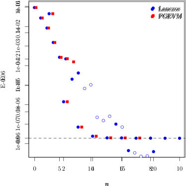
Figure 1: Comparison of PGEVM with $\delta t=1,\Delta=1,t_{0}=0$ and Lanczos for artificial data, see Eq. 18. The PGEVM data is shifted slightly in $x$-direction for legibility. Left: convergence of the ground state energy level as a function of $n$. The exact value is indicated by the dashed line. Right: the difference to the exact ground state energy is plotted on a log-scale as a function of $n$. Empty symbols in the right panel indicate negative differences.

This result confirms that Lanczos and PGEVM are equivalent.

3.2 Nucleon Correlator

Let us now compare Lanczos and PGEVM for a nucleon two-point function obtained from a real lattice QCD simulation. We have used a $N_{f}=2+1+1$ twisted mass lattice ensemble of size $64^{3}\times 128$ with $a\approx 0.08$ fm and $m_{\pi}\approx 130$ MeV Alexandrou:2018egz (21). The correlator $C(t)=\langle N(t)\bar{N}(0)\rangle$ is computed using the local interpolating field $N(x)=\epsilon\,d(x)(u^{T}(x)C\gamma_{5}d(x))$ and projected to zero momentum. We have used $200$ gauge configurations with 16 sources each. First, in the left panel of Fig. 2 we compare Lanczos a,b and c with each other. All three perform very similarly with stable statistical uncertainties also for $n$-values up to $20$, up to some outlier $n$-values for Lanczos b and c. They appear due to the bias correction applied in hindsight after the bootstrap sampling with pivot element has been performed already. For $n>20$ the usage of the pivot mechanism helps in reducing the uncertainties.

All three Lanczos variants share that the plateau is reached around $n=4$. The energy estimate for all larger $n$-values is actually compatible within errors with the estimate at $n=4$, with very little variation. For Lanczos b and Lanczos c there is less increase in the uncertainty, but some outliers appear where the eigenvalue identification apparently failed.

In the right panel of the same figure we compare Lanczos a with the standard $\log$ effective mass Eq. 4. The exponential decrease in the StN ratio is clearly visible for the latter. The plateau for $M_{\mathrm{eff}}$ is reached for $t=10$, using correlator values as $t=10$ and $t=11$. The Lanczos method with $n=4$ uses all correlator values up to $t=7$. Thus, both Lanczos and the $\log$-effective mass reach the plateau once a certain $t$-value is included in the analysis.

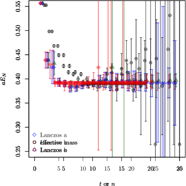
Figure 2: Lanczos results for a nucleon two-point function. Left: comparison of Lanczos a,b,c results as a function of $n$. Right: comparison of Lanczos a with the $\log$ effective mass definition.

When comparing the fluctuations of the expectation value with the uncertainty estimate in Fig. 2 one observes that (apart from the outliers, which are due to eigenvalue misidentification) errors are too large for the data points to be independent. This is better visible in Fig. 3, where we zoom in on the $y$-axis for Lanczos b and indicate a possible plateau fit with the solid line and the error band.

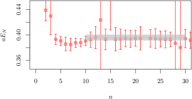
Figure 3: Lanczos b result for the nucleon as a function of $n$ zoomed in on the $y$-axis. The solid line represents a possible plateau fit with error band.

Thus, we next estimate the uncertainty using the double bootstrap as discussed in the previous section. In the left panel of Fig. 4 we plot the ground state energy estimate as a function of $n$ for PGEVM with quantiles as error estimate, and for PGEVM and Lanczos with double bootstrap error estimate.

First of all, it becomes clear from this plot that PGEVM and Lanczos with bias correction yield identical results also for noisy data, apart from a few points where the eigenvalue identification failed. Second, the double bootstrap uncertainty is significantly smaller than the one from quantiles (and, therefore, also outlier removal). Still, even if the error estimates are significantly reduced, fluctuations are too small given the uncertainties for independent data as reported in Ref. Wagman:2024rid (1).

While the estimate of the correlation of results at different $n$-values appears difficult in the presence of (large and many) outliers, the correlation can be computed more reliably on the double bootstrap estimators. This correlation $\mathrm{Cor}(n,n^{\prime})$ is plotted in the right panel of Fig. 4 for four values of $n$ as a function of $n^{\prime}$. At $n=n^{\prime}$ the correlation is identical to 1, as it must be. For $n^{\prime}<n$ we observe an almost linear increase towards 1. For $n^{\prime}>n$, correlation drops quickly, but for large $n$ levels out at a finite plateau value. This finite plateau value increases significantly with $n$, reaching a value of $0.7$ for $n=20$.

A fully correlated, constant fit to the PGEVM (or Lanczos) double bootstrap results in the range from $n=15$ to $n=29$ leads to $aE_{N}=0.395(5)$ with a fairly large $p$-value of $0.999$, indicating again the large correlation among the included data points. A fit to the effective mass data from $t=10$ to $t=18$ results in $aE_{N}=0.390(3)$ and a $p$-value of $0.64$, largely dominated by the effective mass values at $t=10$ to $t=14$. Both fitted values are fully compatible. The value quoted in Ref. Alexandrou:2018egz (21) based on much higher statistics is $aE_{n}=0.3864(9)$.

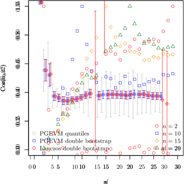
Figure 4: Left: Comparison of PGEVM with error estimate from quantiles, PGEVM with error estimate from double bootstrap and Lanczos with error estimate from double bootstrap. Right: Correlation of the estimates at different $n$-values as a function of $n^{\prime}$.

In order to gain further insight into how the Lanczos method deals with noisy correlator data at large $t$, we have carried out the following experiment: we modify the two-point function by adding to $C(t)$ a Gaussian distributed random shift with width equal to half of the estimated error of $C(t)$. Likewise we modify the bootstrap samples to preserve standard error and correlation and adapt the mean. Then we apply Lanczos to the modified correlator.

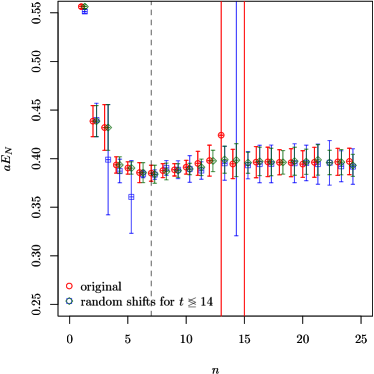
Figure 5: Comparison of Lanczos b applied to the original correlator and to the ones which were modified for $t\leq 14$ (left) and for $t>14$ (right). The vertical dashed line in the right panel indicates the $n$-value from which on modified data enters the result.

The result is shown in Fig. 5, in the left panel the correlator is modified only for $t\leq 14$, in the right panel for $t>14$. Random shifts for $t\leq 14$ are clearly visible in the Lanczos result, while there is almost no change in the Lanczos result on the correlator with modified data for $t>14$. Interestingly, the random shifts for $t>14$ make the outlier disappear in the original Lanczos result. One notes, however, that for both modification scenarios the large $n$-result appears remarkably stable, though still with very little variation of the expectation value relative to the uncertainties.

There is another interesting observation to be made from Fig. 5: random variations of the correlator can cure eigenvalue misidentification problems. For instance in the right panel the results on the randomly shifted correlator for $t>14$ do not show any misidentification issue anymore. This can be used to identify misidentified eigenvalues: one can analyse one or two correlators randomly modified for $t$-values larger than some threshold as discussed above in addition to the original correlator and check for stability of the result.

3.3 Pion Correlator

The pion correlator is, in contrast to the nucleon case, periodic in time. For this case we use a pion correlator for the $N_{f}=2$ Wilson twisted mass ensemble $B_{1}$ from Ref. ETM:2009ztk (22) with $L=24$ and $T=48$. It has a pion mass value of about $300$ MeV at a lattice spacing of $a=0.079$ fm. The correlator estimate is based on $316$ gauge configurations. Note that this data set ships as a sample correlator with the hadron package hadron:2024 (20).

There are two main differences when compared to the nucleon: first, the pion has no signal-to-noise problem; second, the corresponding correlator is periodic. The latter has the consequence that both

$$e^{-E_{0}t}\,,\quad e^{E_{0}t}$$

appear in the spectral decomposition of the correlator with equal amplitudes.

The results of PGEVM and Lanczos, both with double bootstrap error estimate, are compared in the left panel of Fig. 6. For convenience we also plot the usual effective mass estimate $\hat{M}_{\mathrm{eff}}(t=n)$. The general picture appears to be very similar to the nucleon case with the exception of larger fluctuations around $n=10$: this is an effect we attribute to the back propagating state becoming relevant while the matrix size $n$ is not yet sufficient to resolve all relevant states. This effect has been observed already in Ref. Fischer:2020bgv (6).

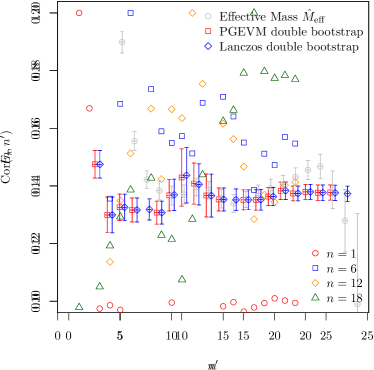
Figure 6: Pion results. Left: ground state pion energy $E_{\pi}$ as a function of $n$ for PGEVM and Lanczos, both with double bootstrap. In grey we we show for comparison $\hat{M}_{\mathrm{eff}}(t=n)$. Lanczos and effective mass data points are slightly shifted horizontally for legibility. Right: correlation estimates like the right panel of Fig. 4, but for the pion.

Moreover, the correlation estimates for the pion correlator are displayed in the right panel of Fig. 6. Qualitatively, the behaviour appears similar to the one of the nucleon correlator shown in the right panel of Fig. 4. However, there are key differences. For $n=6$ correlation starts at zero for $n^{\prime}=1$ and increases to 1 for $n^{\prime}=6$, as expected. Thereafter, the correlation does decrease again until $n^{\prime}=12$. For matrix sizes larger than $12$, the mirror part of the correlator starts contributing, which will likely add little information. This seems to be reflected by a (noisy) plateau in $\mathrm{Cor}(6,n^{\prime})$ for $n^{\prime}>12$.

For $n=12$ the increase from $n^{\prime}=1$ to $n^{\prime}=12$ is present again, but showing a sort of intermediate plateau between $n^{\prime}=7$ and $n^{\prime}=11$, which is the region where the effective mass shows the plateau. For $n^{\prime}>12$ the correlation decreases again with maybe a plateau around values of $0.4$. For $n=18$, finally, instead of the intermediate plateau there is even a minimum in correlation around $n^{\prime}=11$. Only thereafter the correlation rises to $1$. For $n^{\prime}>18$ the correlation plateaus around a value of $0.8$.

Not surprisingly, a fully correlated constant fit to the PGEVM (or Lanczos) results in a range from $n=7$ to $n=22$ basically reproduces the result at $n=22$. The fit result reads $aE_{\pi}=0.1378(24)$ with a reasonable $p$-value of $0.38$. This can be compared to the value $aE_{\pi}=0.1362(7)$ quoted in Ref. ETM:2009ztk (22) based on larger statistics. Both values are fully compatible. If one were to fit the effective mass shown in the left panel of Fig. 6, it really depends on the fit range, but values are also compatible, even though they tend to be higher than the PGEVM result.

4 Discussion

The results presented in the last section clearly demonstrate that (oblique) Lanczos and PGEVM yield identical results, not only for data without noise, but also for noisy data, for which we looked at the nucleon and the pion case separately. The nucleon exhibits the signal-to-noise problem, while the pion is one of the few examples that do not.

By using the double bootstrap estimate of the uncertainty of the median estimator to the expectation value, the correlation of errors of results at $n$ and $n^{\prime}$ can be computed. For the nucleon case they show clearly that the larger $n$ with $n^{\prime}>n$ the results are correlated and the correlation does plateau for $n^{\prime}-n\gtrsim 3$. This plateau value increases with increasing $n$-value.

This behaviour is entirely expected: increasing $n$ by 1 means two more correlator values are included in the analysis. Thus, with increasing $n$ the fraction of additional correlator values with new information decreases like $1/n$. In addition, these correlator values have increasingly large uncertainties. For instance, for $n=20$ there are $40$ correlator values used, and $50$ for $n=25$. Thus, from $n=20$ to $n^{\prime}=25$ the fraction of additional correlator values is $1/5$ and we would expect roughly $80\%$ correlation. We observe a little less. Due to the increasing uncertainties in $C(t)$ itself this correlation is not decreasing anymore and, hence, explaining the plateau.

One might still wonder why the exponentially increasing noise of the correlator values does not lead to an increase in the uncertainties of Lanczos or PGEVM results at large $n$. We explain this as follows: both Lanczos and PGEVM can also work on data with imaginary eigenvalues. And it appears that most of the noise is mapped to those imaginary eigenvalues once the physical eigenvalues are determined sufficiently from correlator values at smaller $t$.

One point worth mentioning here is that eigenvalue identification might still fail despite the methods applied here. We observed in our experiments that random variations of the data can be a way to cure this problem: if after a variation of the correlator within its uncertainties one of the eigenvalues is not found again, it is with high probability a spurious eigenvalue. This could be an alternative to the method described in Ref. Wagman:2024rid (1) where the first row and column of $T_{n}$ are removed, eigenvalues are recalculated, and spurious eigenvalues identified with the same reasoning.

For the pion, on the other hand, without the signal-to-noise problem there appears to be a gain in information up to half of the time extent, after which the correlator is mirrored leading to little additional information.

Finally, we observed for both the pion and the nucleon correlator the behaviour that the PGEVM and Lanczos results show a local minimum at early $n$-values, see Fig. 4 and Fig. 6. Currently, we cannot explain this behaviour.

5 Summary

In this paper we have discussed the equivalence of the Prony GEVM Fischer:2020bgv (6) and Lanczos Wagman:2024rid (1) methods. They are exactly equivalent not only on the analytical level, but also in practice even for noisy data. In particular, both methods converge equally fast to the lattice energy levels one is interested in. We have also seen that double bootstrap is absolutely essential for a robust uncertainty estimate. With double bootstrap and the bootstrap median as the estimator for the expectation value there is also no empirical outlier removal procedure required.

Unfortunately, we conclude from our analysis of the error distributions that the Lanczos method does not solve the signal-to-noise problem. With uncertainties estimated from double bootstrap the correlation of results including correlators at larger and larger $t$-values becomes visible.

One clear advantage PGEVM and Lanczos do have when compared to the standard effective mass is that the result at a large enough $n$-value with its error gives a fit range independent estimate of the energy value. Likely, a model averaging procedure is obsolete in this case. We also observe that both PGEVM and Lanczos provide a lower estimate of the ground state energy level than a plateau fit to the effective mass on the same data. Moreover, this lower value is closer to the estimate obtained with the effective mass approach based on significantly higher statistics.

One should also note that the PGEVM at fixed $n$ scales for large $n$ like $\mathcal{O}(n^{3})$, while the Lanczos method scales only like $\mathcal{O}(n^{2})$. For ensembles with large time extent this is a clear advantage of the Lanczos method. However, PGEVM is more general in principle by adding more degrees of freedom to the algorithm.

Finally, we would like to point out that the block PGEVM introduced in Ref. Fischer:2020bgv (6) should be equivalent to a block Lanczos approach based on the same arguments as discussed in this paper.

References

- (1) Michael L. Wagman “Lanczos, the transfer matrix, and the signal-to-noise problem”, 2024 arXiv:2406.20009 [hep-lat]
- (2) G. P. Lepage “The Analysis Of Algorithms For Lattice Field Theory” Invited lectures given at TASI’89 Summer School, Boulder, CO, Jun 4-30, 1989. Published in Boulder ASI 1989:97-120 (QCD161:T45:1989), 1989
- (3) Christopher Michael and I. Teasdale “Extracting Glueball Masses From Lattice QCD” In Nucl. Phys. B215, 1983, pp. 433–446 DOI: 10.1016/0550-3213(83)90674-0
- (4) Martin Lüscher and Ulli Wolff “How to Calculate the Elastic Scattering Matrix in Two-dimensional Quantum Field Theories by Numerical Simulation” In Nucl. Phys. B339, 1990, pp. 222–252 DOI: 10.1016/0550-3213(90)90540-T
- (5) Benoit Blossier, Michele Della Morte, Georg Hippel, Tereza Mendes and Rainer Sommer “On the generalized eigenvalue method for energies and matrix elements in lattice field theory” In JHEP 04, 2009, pp. 094 DOI: 10.1088/1126-6708/2009/04/094
- (6) Matthias Fischer, Bartosz Kostrzewa, Johann Ostmeyer, Konstantin Ottnad, Martin Ueding and Carsten Urbach “On the generalised eigenvalue method and its relation to Prony and generalised pencil of function methods” In Eur. Phys. J. A 56.8, 2020, pp. 206 DOI: 10.1140/epja/s10050-020-00205-w
- (7) G. R. Prony In Journal de l’cole Polytechnique 1.22, 1795, pp. 24–76
- (8) S. Romiti and S. Simula “Extraction of multiple exponential signals from lattice correlation functions” In Phys. Rev. D 100.5, 2019, pp. 054515 DOI: 10.1103/PhysRevD.100.054515
- (9) Daniel C. Hackett and Michael L. Wagman “Lanczos for lattice QCD matrix elements”, 2024 arXiv:2407.21777 [hep-lat]
- (10) George Tamminga Fleming “What can lattice QCD theorists learn from NMR spectroscopists?” In QCD and numerical analysis III. Proceedings, 3rd International Workshop, Edinburgh, UK, June 30-July 4, 2003, 2004, pp. 143–152 arXiv: http://www1.jlab.org/Ul/publications/view_pub.cfm?pub_id=5245
- (11) Silas R. Beane, William Detmold, Thomas C. Luu, Kostas Orginos, Assumpta Parreno, Martin J. Savage, Aaron Torok and Andre Walker-Loud “High Statistics Analysis using Anisotropic Clover Lattices: (I) Single Hadron Correlation Functions” In Phys. Rev. D 79, 2009, pp. 114502 DOI: 10.1103/PhysRevD.79.114502
- (12) Kimmy K. Cushman and George T. Fleming “Automated label flows for excited states of correlation functions in lattice gauge theory”, 2019 arXiv:1912.08205 [hep-lat]
- (13) Kimmy K. Cushman and George T. Fleming “Prony methods for extracting excited states” In Proceedings, 36th International Symposium on Lattice Field Theory (Lattice 2018): East Lansing, MI, United States, July 22-28, 2018 LATTICE2018, 2019, pp. 297 DOI: 10.22323/1.334.0297
- (14) George T. Fleming “Beyond Generalized Eigenvalues in Lattice Quantum Field Theory” In 40th International Symposium on Lattice Field Theory, 2023 arXiv:2309.05111 [hep-lat]
- (15) Konstantin Ottnad, Tim Harris, Harvey Meyer, Georg Hippel, Jonas Wilhelm and Hartmut Wittig “Nucleon average quark momentum fraction with Wilson fermions” In EPJ Web Conf. 175, 2018, pp. 06026 DOI: 10.1051/epjconf/201817506026
- (16) Shmuel Kaniel “Estimates for Some Computational Techniques in Linear Algebra” In Mathematics of Computation 20.95 American Mathematical Society, 1966, pp. 369–378 URL: http://www.jstor.org/stable/2003590
- (17) Christopher C. Paige “The computation of eigenvalues and eigenvectors of very large sparse matrices”, 1971 URL: https://www.cs.mcgill.ca/~chris/pubClassic/PaigeThesis.pdf
- (18) Y. Saad “On the Rates of Convergence of the Lanczos and the Block-Lanczos Methods” In SIAM Journal on Numerical Analysis 17.5 Society for IndustrialApplied Mathematics, 1980, pp. 687–706 URL: http://www.jstor.org/stable/2156670
- (19) B. Efron and R.J. Tibshirani “An introduction to the bootstrap” ChapmanHall/CRC, 1994
- (20) Bartosz Kostrzewa, Johann Ostmeyer, Martin Ueding and Carsten Urbach “hadron: package to extract hadronic quantities” R package version 3.3.1, https://github.com/HISKP-LQCD/hadron, 2024 URL: https://github.com/HISKP-LQCD/hadron
- (21) Constantia Alexandrou “Simulating twisted mass fermions at physical light, strange and charm quark masses” In Phys. Rev. D 98.5, 2018, pp. 054518 DOI: 10.1103/PhysRevD.98.054518
- (22) Remi Baron “Light Meson Physics from Maximally Twisted Mass Lattice QCD” In JHEP 08, 2010, pp. 097 DOI: 10.1007/JHEP08(2010)097
- (23) R Core Team “R: A Language and Environment for Statistical Computing”, 2019 R Foundation for Statistical Computing URL: https://www.R-project.org/