Large Multi-modal Models Can Interpret Features in Large Multi-modal Models

Abstract

Recent advances in Large Multimodal Models (LMMs) lead to significant breakthroughs in both academia and industry. One question that arises is how we, as humans, can understand their internal neural representations. This paper takes an initial step towards addressing this question by presenting a versatile framework to identify and interpret the semantics within LMMs. Specifically, 1) we first apply a Sparse Autoencoder (SAE) to disentangle the representations into human understandable features. 2) We then present an automatic interpretation framework to interpreted the open-semantic features learned in SAE by the LMMs themselves. We employ this framework to analyze the LLaVA-NeXT-8B model using the LLaVA-OV-72B model and demonstrate that these features can effectively steer the model’s behavior. Our results contribute to a deeper understanding of why LMMs excel in specific tasks, including EQ tests, and illuminate the nature of their mistakes along with potential strategies for their rectification. These findings offer new insights into the internal mechanisms of LMMs and suggest parallels with cognitive process of the human brain. We opensource our codebase and checkpoints at Github

1 Introduction

Recently Large Multi-modal Models (LMMs) [21, 20, 8, 3, 36] have significantly advanced the field of computer vision, achieving remarkable success in various applications such as personal assistant, medical diagnosis, and embodied agents [39, 24]. These models have been integrated into commercial products to assist people’s daily life [2, 26] and hold large potential to transform the future. Despite their success, the opaque nature of LMMs often leads to unexpected behaviors, such as the hallucination of non-existent objects and relationships within images [14], as well as vulnerability to jailbreak attacks [7, 33]. These challenges underscore the critical importance of understanding and controlling the neural representations of LMMs.

Interpreting LMMs presents several challenges compared to traditional models. One key challenge is the high-dimensional, polysemantic nature of their representations. A single neuron within these networks may encode multiple semantics, while a single semantic can also be distributed across multiple neurons [29, 11]. For example, a neuron in the vision features of Inception v1 can respond to both cat faces and car fronts [28]. The larger dimensionality of LMMs compared to conventional models adds more complexity. An efficient algorithm is needed to decompose neural representations into basic components. The second challenge is the vast and open-ended concepts in LMMs. Traditional models, which contain only hundreds of monosemantic concepts such as color, objects, attributes, and layout [42, 4, 34, 31], can be analyzed through extensive human labeling, enabling interpretation of neural representations based on these specific concepts. In contrast, LMMs contain hundreds of thousands of monosemantic concepts across open domains, making human analysis infeasible. This calls for a zero-shot approach to detect the concepts, which minimizes human effort.

Existing works, such as [13, 5], have demonstrated that larger models, like GPT-4, can be used to interpret neurons in smaller models, such as GPT-2. In this paper, we take an initial step toward exploring this approach in the domain of LMMs. We aim to dissect and understand open-semantic features by applying similar methods to analyze LLaVA-NeXT-8B with the larger LLaVA-OV-72B model. We employ sparse auto-encoders (SAEs) [30, 10], a classic interpretability method, to address the first challenge of polysemantic neurons by disentangling them into human-understandable features. In previous works such as [18, 13, 35, 6], the learned features in SAE are proven to be more monosemantic and human-understandable than the neurons. For the second challenge, we develop a pipeline for automatic feature discovery in SAEs, taking advantage of LMMs’ zero-shot abilities. Specifically, for a specific learned feature in SAEs, we first identify Top-K images and the areas in those images that mostly activate on the feature. Then the images and patches will be fed into LLaVA-OV-72B [17] to examine the common factors and generate explanations.

In addition to methodological contributions, our case studies also offer unique insights into LMMs. Firstly, we identify emotional features in LMMs and demonstrate that these features enable LMMs to generate or share emotions. Previous works have highlighted the exceptional capabilities of LMMs in EQ assessments [39] and their ability to read emotions. We extend this investigation by exploring the emotions of LMMs and steering the model to express its own feelings. Secondly, we identify the causes of certain model behaviors and analyze potential reasons for undesired outcomes, such as hallucinations. Adjusting the relevant features can rectify the mistake. Thirdly, some features in LMMs align with those found in the human brain, suggesting that interpreting LMMs could be informative for understanding how the human brain integrates multisensory inputs. For example, we find features that are activated by an action and their corresponding OCR descriptions, which align with the invariant visual features found in the study by [32]. Specifically, our contributions can be summarized as follows:

• We introduce the use of Sparse Autoencoders (SAEs) to analyze the open-semantic features of Large Multimodal Models (LMMs) and demonstrate, for the first time in multimodal domain, that the features learned by SAE in a smaller LMM can be effectively interpreted by a larger LMM.

• We propose an automated pipeline for interpreting these features and further demonstrate that they can be used to steer model behaviors to address specific issues or induce desired outputs.

• Additionally, we propose a method for identifying the underlying causes of model behaviors and offer an analysis of how to address these issues, highlighting the potential for developing more reliable LMMs.

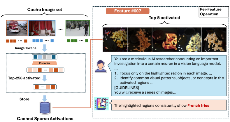
Figure 2: The overview of the explanation pipeline, where images are forwarded through the LMM with the integrated SAE, and the activations of the top 256 most activated features are cached. For each feature, the top 5 images with the highest activations are selected, followed by the execution of zero-shot image explanations using a large LMM.

2 Methodology

In this section, we present our methodology to disentangle, interpret, and steer the internal representation of LMMs.

2.1 Sparse Auto-encoders for Disentanglement

Architecture and loss function:

We utilize the SAE architecture outlined in OpenAI’s research [13], which consists of a two-layer auto-encoder with a TopK activation function. Let’s denote the input by $\bm{x}\in\mathbb{R}^{T\times d_{l}}$, where $T$ is the number of tokens and $d_{l}$ is the hidden dimension of Llava. The SAE operates as follows:

$$\bm{z}=\text{TopK}(\text{ReLU}(\bm{W}_{1}(\bm{x}-\bm{b}_{1})+\bm{b}_{2})),$$ (1)

$$\hat{\bm{x}}=\bm{W}_{2}\bm{z}+\bm{b}_{3},$$ (2)

where $\bm{z}\in\mathbb{R}^{T\times d_{s}}$, where $d_{s}$ is the hidden dimension of SAE, represents the sparse data representation, $\hat{\bm{x}}$ is the reconstructed data, and the sets $\{\bm{W}_{i},\bm{b}_{i}\}$ are the trainable parameters. The loss function combines the reconstruction error with an auxiliary loss used in [13] to prevent inactive features in $\bm{z}$.

To understand why SAEs yield monosemantic features, we draw parallels between the components in (1) and those in traditional sparse coding [30, 10]. In this context, $\bm{W}_{2}$ acts as an overcomplete dictionary [1] for the input data, with its rows forming the dictionary vectors, and $\bm{z}$ serving as the sparse coefficients corresponding to these vectors. Due to the sparsity of $\bm{z}$, the dictionary vectors tend to be nearly orthogonal (or mutually incoherent) to minimize reconstruction error. This near orthogonality suggests that the dictionary vectors are almost independent and each coordinate of $\bm{z}$ is expected to be monosemantic.

Integrating SAEs into LLaVA:

We incorporate SAE into a specific layer of LLaVA, where the hidden representation corresponds to $\bm{x}$ in (1). The SAE is trained using the LLaVA-NeXT [20, 16] sft dataset, which contains approximately 779k samples. During forward, we always use the Anyres [20] strategy to process the image tokens.

2.2 Zero-shot Identification of Concepts

To identify the open-semantic features, we present a pipeline leveraging open-source Large Multimodal Models (LMMs) to identify concepts within LMMs. In this subsection, we only consider the 576 base image features when preparing the exemplars.

Identifying the Top Activated Images and Patches:

Initially, we pinpoint the most activated images for each coordinate in the latent space vector $\bm{z}$. Due to computational resource constraints, we cache a subset of images from the LLaVA training dataset and augment it with images from additional datasets [12, 40, 19, 16], with a total $46684$ images, collectively denoted as $\mathcal{D}$. These images are processed through LLaVA to yield the representation $\bm{X}\in\mathbb{R}^{|\mathcal{D}|\times 576\times d}$. The corresponding latent representation in the SAE is $\bm{Z}\in\mathbb{R}^{|\mathcal{D}|\times 576\times d_{s}}$. By averaging over the second dimension, we obtain the mean activation values $\bar{\bm{Z}}=\frac{1}{576}\sum_{j}\bm{Z}[:,j,:]\in\mathbb{R}^{|\mathcal{D}|\times d_{s}}$. For each feature in the SAE, we identify the top-5 influential image by selecting the top-5 activations along the first dimension of $\bar{\bm{Z}}$. To determine the specific patch that activates a feature, we process the top-k most influential image through LMMs to obtain its representation $\bm{x}\in\mathbb{R}^{5\times 576\times d}$ and its corresponding SAE latent for a feature $\bm{Z_{i}}\in\mathbb{R}^{5\times 576}$ where $i$ represent one of the feature in $d_{s}$. In real time, since we are using a Top-K SAE, we can cache the $\bm{Z}$ using a sparse vector $V\in\mathbb{R}^{|\mathcal{D}|\times 576\times k}$ by selecting the Top-K features from the last dimension and reduce the forward number.

Automatic Feature Interpretation of LMMs by LMMs:

We apply masks to the top activated images, using transparent masks for the most activated patches and black masks for the rest. These masked images are then input into LLaVA-NeXT-OV-72B [17] to detect common patterns. If no common patterns are discernible, the system will return a message stating “unable to produce explanations”. We demonstrate the overall procedure of our explanation pipeline in Fig. 2.

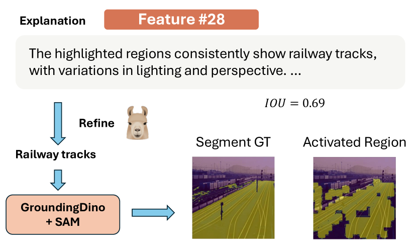
Figure 3: An overview of the evaluation pipeline for calculating IOU scores. Initially, a small LLM is used to refine the explanation into a concise description, which is then employed to generate the segmentation mask. The IOU score is subsequently computed by comparing the mask to the binarized activated region.

Reference Score Calculation:

To quantify the relevance of a feature’s activation to a given concept, we first refine the descriptive text using language models to enhance conciseness. For instance, the verbose description ”The feature activates on the train tracks …” is condensed to ”Train tracks”. This refinement is performed with a smaller LLM to minimize computational expense and time. Following this, GroundingDino-SAM [22] is employed to generate a segmentation mask based on the succinct interpretation. Subsequently, we construct a composite mask incorporating every object detected in the image. The IoU score between the segmentation mask and our activation mask is then calculated, serving as the reference score for the feature’s relevance. An example of the evaluation process is demonstrated in Fig. 3 where the refined explanation is being sent to the GroundingDino-SAM [22] to produce the segmentation ground truth and calculate the IOU with the activated region.

2.3 Steering the Neural Representation

Having interpreted each representation in the SAEs, we explore how to influence the output by steering a specific feature within the SAEs. Steering involves adjusting the feature’s value, either increasing or decreasing it. Specifically, steering in SAEs entails setting the $i$-th hidden representation to a predetermined value $k$. We define the steering operation $\text{Steer}(\mathcal{C},k,i)$ in SAEs as follows:

$$\bm{z}=\text{ReLU}(\bm{W}_{1}(\bm{x}-\bm{b}_{1})+\bm{b}_{2}),$$ (3)

$$\bm{z}[\mathcal{C},j]=k$$ (4)

$$\hat{\bm{z}}=\text{TopK}(z),$$ (5)

$$\hat{\bm{x}}=\bm{W}_{2}\hat{\bm{z}}+\bm{b}_{3},$$ (6)

where $\mathcal{C}$ represents the set of tokens designated for steering, $k$ is the steering value, and $j$ is the index of the feature in the SAE to be steered. Following the steering operation, we input $\hat{\bm{x}}$ into the subsequent LLaVA layer instead of $\bm{x}$. In the experiments discussed in Section 4.1, we apply steering to all tokens by setting $\mathcal{C}$ accordingly. This steering operation is further utilized in the subsequent subsection.

2.4 Localizing the Causes for Model Behaviors

In scenarios where LMMs make decisions, it is often crucial to discern whether these decisions are influenced by vision-related tokens and to determine which specific features are activated. We follow similar approaches in [37, 27, 35] and introduces the technique to identify such relationships in this subsection.

We assume the input comprises $T$ tokens and the model begins outputting from the $(T+1)$-th token, with the decision represented by a single token. We denote the output logits for the $(T+1)$-th token as $\bm{u}$, the current output token id as $v_{c}=\text{argmax}(\bm{u})$, and a baseline token id as $v_{b}$. Our objective is to ascertain why the LMMs exhibit a preference for $v_{c}$ over $v_{b}$. The difference in logits is defined as:

$$d(\bm{u},v_{c},v_{b})=\bm{u}[v_{c}]-\bm{u}[v_{b}].$$

To locate the causes for the decision, we iterate over every patch and every hidden feature in the SAE. The process involves three steps for each token $i$ and each SAE feature $j$: 1. Apply $\text{Steer}(i,j,0)$ to negate the feature’s impact. 2. Process the modified input through Llava to obtain new logits $\hat{\bm{u}}$. 3. Calculate the influence of the $j$-th feature in the $i$-th token on the decision preference for $v_{c}$ over $v_{b}$:

$$I(i,j,v_{c},v_{b})=d(\hat{\bm{u}},v_{c},v_{b})-d(\bm{u},v_{c},v_{b}).$$

Given the time-intensive nature of this method due to multiple forward passes, we employ a linear approximation with the method in [27]:

$$I(i,j,v_{c},v_{b})\approx\left(\frac{\partial d(\bm{u})}{\partial\bm{z}}\right)^{T}(\hat{\bm{z}}-\bm{z}),$$

where $\hat{\bm{z}}$ is the SAE’s activation post-steering operation. This approximation allows us to estimate attribution of each token as illustrated in [27].

3 Experiments

3.1 Scaling SAEs for LMMs

Dataset and Model Setups: We choose the LLaVA-NeXT-LLaMA3-8B  [16] as our base model and hooked the SAE on the $25^{th}$ layer and use the same fine-tuning data from LLaVA-NeXT [20] for training. During training, unlike previous works [35, 6, 13] that used a pretrained format text, we format the text and image into ways that looks exactly the same as the supervised fine-tuning stage. We scale our sparse autoencoder with $2^{17}$ with 8 batch size and 4 gradient accumulation steps. We later tries to scale the features into $2^{18}$ but observe no loss decrease. We use the same Top-k sparse autoencoder settings as  Gao et al. [13], Makhzani and Frey [25] and select $k=256$ that similar to the activated features in [35]. Unless otherwise specified, we will use the settings of SAE with $2^{17}$ features for the rest of this paper. The reason that we choose this large number of features is that we wish our feature to be more splited and informative as similar in the approaches in [1, 35].

3.2 Interpretaion Pipeline Evaluation

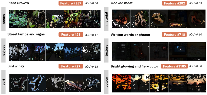
Figure 4: A comparison of several visual concepts and their activated areas. We compare several visual concepts and their corresponding activated areas, showcasing one example for each concept across different features. For each feature, we calculate the IOU by averaging the IOUs from the top-5 activated images. Although some features yield relatively low IOU scores, we find that the explanations are still semantically accurate with respect to the activated regions.

Concept	Metric	Random	V-Interp (Ours)
scene	IOU $(\uparrow)$	$0.007\pm 1\times 10^{-3}$	0.20
	CS $(\uparrow)$	$18.1\pm 6\times 10^{-2}$	24.4
object	IOU $(\uparrow)$	$0.005\pm 5\times 10^{-4}$	0.19
	CS $(\uparrow)$	$18.2\pm 2\times 10^{-2}$	24.0
part	IOU $(\uparrow)$	$0.007\pm 2\times 10^{-3}$	0.21
	CS $(\uparrow)$	$18.1\pm 5\times 10^{-2}$	23.5
material	IOU $(\uparrow)$	$0.01\pm 8\times 10^{-3}$	0.39
	CS $(\uparrow)$	$18.1\pm 1\times 10^{-1}$	24.1
texture	IOU $(\uparrow)$	$0.007\pm 2\times 10^{-3}$	0.21
	CS $(\uparrow)$	$18.4\pm 6\times 10^{-2}$	20.9
colour	IOU $(\uparrow)$	$0.005\pm 2\times 10^{-3}$	0.10
	CS $(\uparrow)$	$19.6\pm 7\times 10^{-2}$	20.3
Total	IOU $(\uparrow)$	$0.005\pm 2\times 10^{-4}$	0.20
	CS $(\uparrow)$	$18.2\pm 1\times 10^{-2}$	23.6

Table 1: The Intersection over Union (IoU) and CLIP scores for each concept are computed based on the top-5 most activated images.

	scene	object	part	material	texture	colour	Total
GPT-4o	0.93	0.84	0.9	1.0	0.85	0.92	0.89
Human	0.70	0.85	0.60	0.95	0.80	0.60	0.75

Table 2: Consistency scores for our explanation, computed based on 100 samples per concept for GPT-4o consistency and 10 samples for human consistency, highlighting the agreement between GPT-4o-generated and human-generated explanations.

Results

We present our result in Tab. 1. Due to the same limitation as illustrate in [35, 6], we report the result on a 5000 subset of features with around 46684 images for caching the features’ activations. For the random result, we randomly sampled 5 images from the cache dataset and run 10 times for IOU and 30 times for the CLIP-Score. We then reported the average result of each run along with the 99% confidence interval. We followed the concepts used in [4] and utilize LLaMA-3.1-Instruct-70B [9] to help us label the concept according to its explanation. In Fig. 4, we also present examples that demonstrate the activated region for different concepts and report the IOU scores for each example.

Consistency

We present the consistency scores for each concept in Tab. 2. To evaluate the consistency of our explanations with the activated image regions, we employ GPT-4 as a judge and conduct a human study. For GPT consistency, we sample 100 test cases per concept, provided that the total number of samples for the concept exceeds 100. For human consistency, we manually label the correctness of 10 samples for each concept.

4 Probing into the Features

In previous section, we demonstrate that we are able to locate and interpret the visual features in a LMM using an automatic pipeline. However, what differs LMM from traditional vision model is its conversation, reasoning, and generalization ability across different modalities. On other words, we believe that the features inside LMM are open-semantic and should not be limited into the concepts in [4]. In this section, we probe into the features in our SAE and try to find out how different features contribute to the final result, and how can these features being used to steer model’s behavior in different scenarioes.

4.1 Case Studies of Emotion Feature

When interacting with humans, it is essential for the model to demonstrate empathy and the ability to understand human emotions. In [39], it has been shown that large multimodal models (LMMs) can perceive emotions and Emotional Quotient (EQ), enabling them to understand and resonate with human feelings. Building on this, we specifically investigate the relevant features, exploring how the model comprehends these features and how they influence its reasoning processes. Through examples of various image features and their effects on model responses, we demonstrate that LMMs are capable of: 1) Connecting emotional concepts between text and visual features, such as actions and behaviors; 2) Engaging with human emotions by adjusting the corresponding features to intervene in the reasoning process manually. 3) Response to concept that with invariant features between modalities.

Figure 5: The feature that relates to sad. We probe and find out the feature that activated on ”sad”. By clamping this feature, we can enforce the model to share the feeling of sad

Sad

We present a feature that may be related to the feeling of ”sadness” and explore the potential for enabling the model to share emotional responses. After probing and confirming that the feature aligns with ”sadness,” we investigate whether manipulating this feature could influence the model’s reasoning to simulate emotional responses. To test this, we use a simple prompt, ”What is your feeling right now?” and ask the assistant. Without steering, the model responds in a neutral, standard AI assistant tone, showing no emotion. However, when we clamp the ”sad” feature to a high value, the model responds with ”sad” as shown in Fig. 5

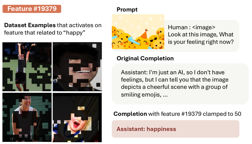
Figure 6: The feature that relates to happy. We find out that the feature is related with joy and celebrate action that relate to happiness. By clamping this feature, we can enforce the model to share the feeling happiness with others.

Happy

Beyond simply experiencing a feeling, it is also essential for the LMM to interact and share emotions when presented with a specific scenario. Toward this goal, we use the same method to probe the feature associated with ”happiness” and provide an image depicting a joyful scenario. When asked about its feelings without steering, the model responds that it does not experience emotions. However, similar to the ”sad” feature, when we clamp the ”happy” feature, the model responds with expressions of happiness, as shown in Fig. 6. This demonstrates that the model’s reasoning process can be effectively influenced.

Hungry, Greedy

We discovered an intriguing feature that links the text-based emotional concepts of greedy and hungry to visual representations of the action eating and the word hungry. We notice that the feature activates in response to the word hungry in the image, suggesting that it connects not only to the action eat but can also extend to broader concepts. To test this, we clamp this feature and prompt the model with ”Tell me a story about Alice and Bob”; the generated response revolves around themes of greed as shown in Fig. 7. This demonstrates that the model can reason from the visual action eat to a broader concept encompassing greedy and hungry with a unified view.

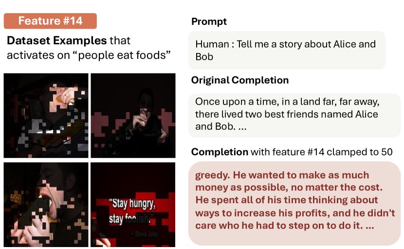
Figure 7: A feature that relates to the concept ”eat”. We further investigate about the concept behind this feature and find out that model can reason from a visual action ”eat” into the concept ”concept” and ”greedy”

4.2 Low Level Perception Features

One important distinction we observed in our features, as compared to those found in Large Language Models in previous studies [35, 6, 13], is the presence of numerous low-level visual features. These features typically represent basic concepts related to common visual elements and often exhibit high activation across most images. For example, these features may be associated with color, shape, or fundamental visual patterns, such as mesh structures or repetitive designs. In the example shown in Fig. 6, the feature associated with ”happy” is only the 78th most activated feature, with many other low-level concepts present as well. We showcase some of these features in Sec. 12, highlighting a key difference between LMMs and LLMs.

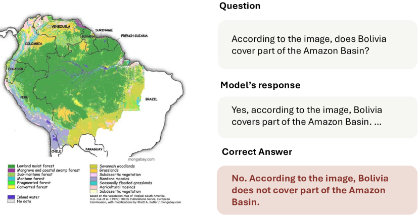
Figure 8: An example of the hallucination on LLaVA. Bolivia is not shown on the image but the model still answer yes.

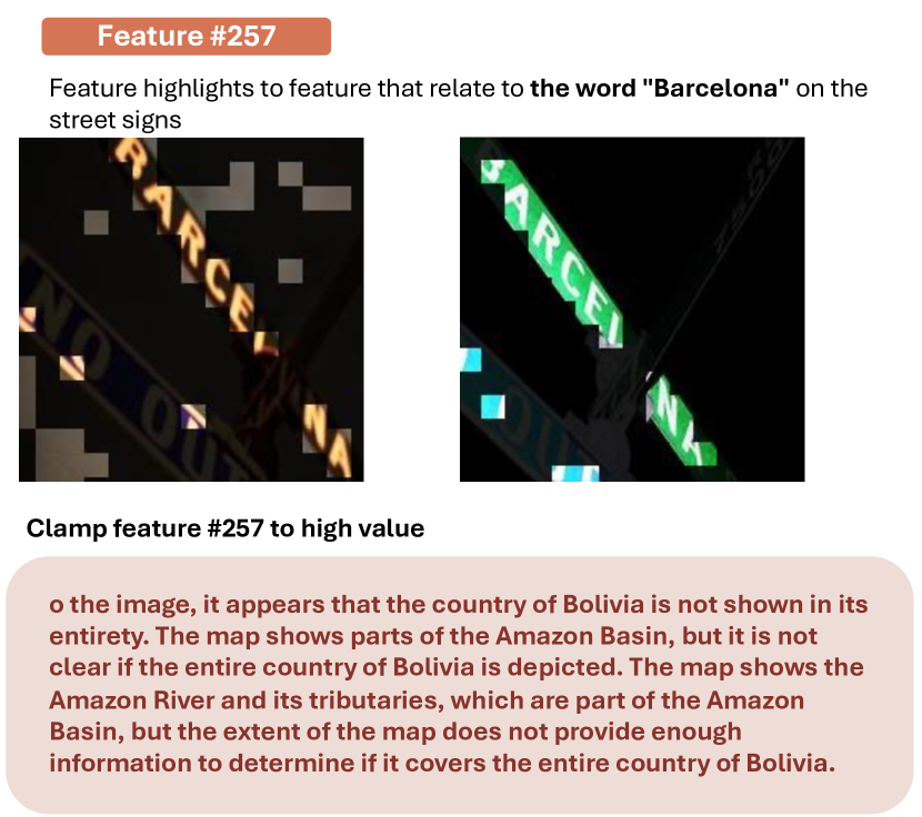
Figure 9: Feature that relates to the text ”Barcelona”. By clamping this feature to high value, we intervene the reasoning steps and hallucination in Fig. 8 disappears.

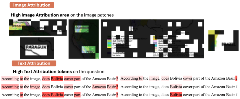
Figure 10: The high attribution area of different images and on the text. For images, we observe that features with high attribution mostly activate on positions that relate to key information about the question. For text, we observe that the ”Bolivia” token contributes the most to the answer ”yes”

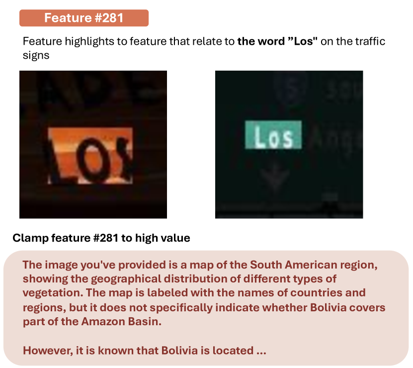
Figure 11: Feature that relates to the text ”Los”. We validate our assumption by finding another feature that relates to text and mitigate the hallucination.

4.3 Localizing the Cause for Model Behaviors

In Sec. 2.4, we mention the patching method that used to locate the cause for the model’s output. This has been treated as viewing the features as model’s intermediate steps in [35]. In this section, we use a hallucination example to deeply study this process in LMM. As shown in Fig. 8, we provide an example from HallusionBench [14] that LLaVA hallucinates on the image and answer Yes even if the image does not shown anything about Bolivia.

To study the cause for this output, we set the answer token $v_{c}=yes$ and $v_{b}=no$ and apply the algorithm with calculate per token contribution. By employing this strategy, we can filter out features that causing the model to be more favored to answer ”yes” instead of answer ”no”. To be specifically in this case, we mainly focus on two points: 1) How does the model reason from the image and is the model reason from the correct path? 2) If the model is paying the correct attention in the image, which part of the text part is causing the hallucination. To answer these two questions, we sort features by their attribution effect on image and text separately and observe their common part with high attribution.

Image Attribution

In Fig. 10, we visualize image patches for common areas with high attribution among the features. To do this, we first filtered out the top 10 features with the highest attribution towards the final output ”yes” and visualized their attribution map. Examining these top features reveals that they primarily contribute to tokens associated with text elements, such as map legends, country names, and other key visual details. This observation demonstrates that the model is effectively focusing on relevant areas of the image and has the ability to accurately identifying where to extract necessary information. However, even with the correct visual perception ability, the model still fail to produce the final answer.

Text Attribution

To further investigate the source of the incorrect answer, we continue visualizing the attribution of text tokens in the question. As shown in Fig. 10, the token ”Bolivia” contributes most to features with high attribution toward the answer ”yes.” Additionally, tokens like ”to” and ”the,” along with concepts such as ”Amazon Basin,” also have a positive attribution to the hallucinated answer ”yes.” This partially explains why the model responds with ”yes” instead of ”no,” even after extracting useful information from the image. While reasoning from visual features, the model is also influenced by text, leading it to approach the question with its pretrained knowledge.

4.4 Application of Model Steering on Hallucination

After identifying the cause for causing the hallucination, we start to wonder how can we fix this hallucination by using steering. We are now assure that the model has the ability of reading the image as it can focus on the correct part of the image but it is being affected by the text tokens and approaches the question without answering the question on image. In this subsection, we focus on how can we utilize the steering effect to intervene the reasoning steps for the model to get the correct answer.

To address this issue, we first consider which features can encourage the model to focus on text tokens in the image rather than the question text. We hypothesize that clamping activations for certain OCR features related to image text may prompt the model to prioritize image-based features over question text features. We identify two such features that reduce hallucinations. In Fig. 9, we locate a feature linked to the word ”Barcelona” and clamp it to a high value, leading the model to rely on image information rather than general geographical knowledge. To validate this, we identify a feature related to the word ”Los” on traffic signs and similarly clamp it in Fig. 11, prompting the model to conclude that Bolivia is absent in the image. This shows that the model can use image information but may sometimes follow incorrect reasoning. With minimal intervention, we successfully guide the model to prioritize image information over question text.

5 Conclusion

In summary, we present an in-depth examination on the internal structure of the LMM and introduce an automated pipeline for interpreting its open-semantic features. Furthermore, we propose methods for steering the model’s behavior through these features and for identifying the sources of errors within the LMM. By systematically analyzing both the structural and functional aspects of the model, we aim to offer valuable insights into its interpretability and reliability. We hope that these findings will not only contribute to the advancement of research in this area but also stimulate further exploration into this area.

Supplementary Material

6 Related Works

Dictionary Learning

Dictionary learning is a common approach for problems like ours, where we aim to extract a set of features from a collection of dense vectors. Sparse autoencoders (SAEs), proposed by [30, 10], have been used as a classic interpretability method to address this challenge. SAEs are designed to identify mutually incoherent bases in data and represent the data as sparse linear combinations of these bases. Existing studies have applied SAEs to LLMs, finding that the bases represent monosemantic features in the data, with the coefficients indicating the activation of these features[18, 13, 35].

Large Multimodal Models

With the development of large language models (LLMs), the performance of large multimodal models has also advanced rapidly, demonstrating strong results across various tasks [16, 20, 3, 38]. Studies such as  [31, 23] have explored methods to understand or manipulate the internal structure of LMMs. In our work, we take an initial step toward evaluating and interpreting the open-semantic features within LMMs.

7 Limitations

Our work primarily focuses on the LLaVA-NeXT-LLaMA-8B model and a specific layer within it. This focus on a particular model and layer is based on the assumption of universality and disentanglement, as discussed in [35, 6]. However, this assumption may contribute to inaccuracies in interpretation and model steering.

Due to limitations in computational complexity and storage, we were unable to prepare a sufficiently large and diverse cached image dataset to accurately interpret the image features. Consequently, we present our results on a subset of features and may have mistakenly classified some features as inactive.

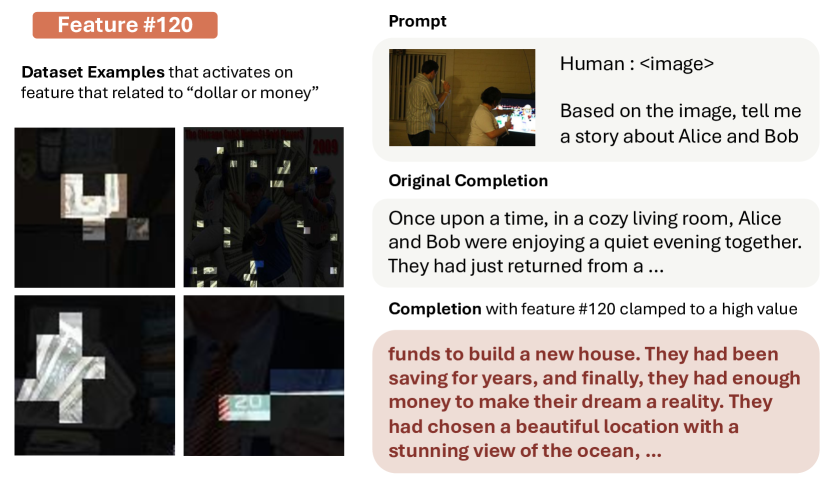
Figure 12: The feature related to money and its steering effect.

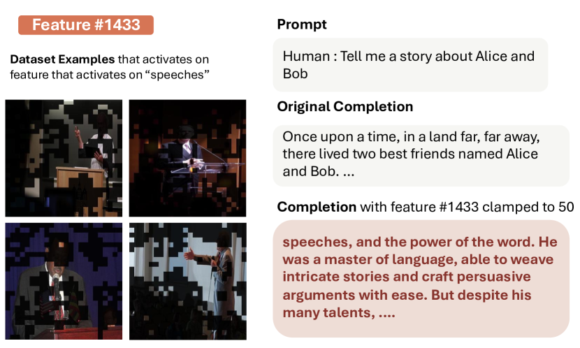
Figure 13: The feature related to speech and its steering effect.

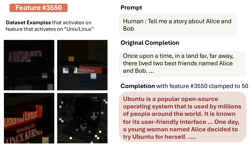
Figure 14: The feature related to unix and its steering effect.

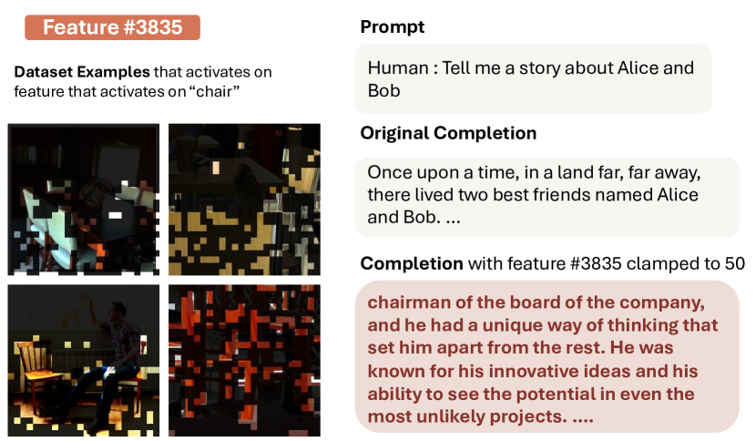
Figure 15: The feature related to chair and its steering effect.

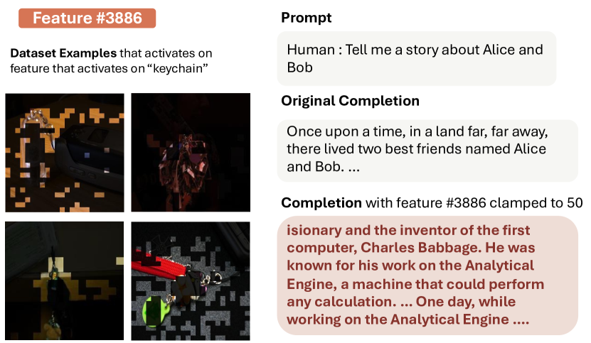
Figure 16: The feature related to money and its steering effect.

8 Detail about Prompt

We detail the prompts used in different stages of the automated pipeline in this section. The prompt for zero-shot identification of concepts is provided in Tab. 3. For this task, we utilize the LLaVA-NeXT-OV-72B model [17]. To refine labels and categorize explanations using large language models (LLMs), we use the prompts detailed in Tabs. 5 and 6. Specifically, LLaMA-3.1-Instruct-8B is used for label refinement, while LLaMA-3.1-Instruct-70B is employed for categorizing explanations. For high-throughput performance, the models are served using SGLang [41].

Table 3: The prompt for zero-shot identification of concepts

Table 4: The prompt to ask GPT to evaluate the correctness of the evaluation

Table 5: The prompt that use to label concept for each description

Table 6: The prompt that used to refine the explanations for grounding and segment visual objects

9 More Steering Examples

In this section, we provide more steering examples that we discover during experiments. We perform a large scale steering on the 5000 size features subset we choose and then filtered some interesting examples here. In Fig. 12, the feature activates on money and when this feature is clamped to 50, the model output a story about saving funds and by a house. In Fig. 13, when a feature relates to a feature that relate to speech, the model output a story about a man who is a speech master. In Fig. 14, we found a feature that relate to unix/linux and its steering effect would output a story about Ubuntu. More interestingly, in Fig. 15, though the model response on a visual ”chair” object, when steering this feature, model would output a story relates to ”chairman” instead of a ”chair”. Another example is that in Fig. 16, when steering this feature related to ”key” or ”keychain”, the model output a story about developing some analytic software.

10 CLIP-Score and IOU details

We use Grounding DINO L [22] as our grounding module and SAM Huge [15] as our segment module. The output from the interpretation pipeline is being refined into concise description by using the LLaMA-3.1-Instruct-8B [9]. We use ViT-B/32 CLIP model to generate embeddings and calculate the cosine similarity between the interpretations and the image. We calculate the IOU and the CLIP-Score using the top-5 activated images for each features. Due to the same limitation as illustrate in [35, 6], we report the result on a 5000 subset of features with around 46684 images for caching the features’ activations.

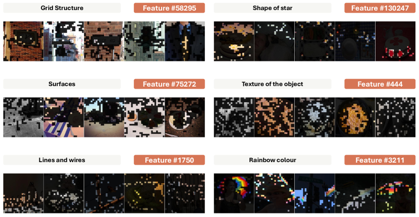
Figure 17: Low level features in the LMM. These features activate in most of the images and showcase the model’s basic cognition and perception abilities.

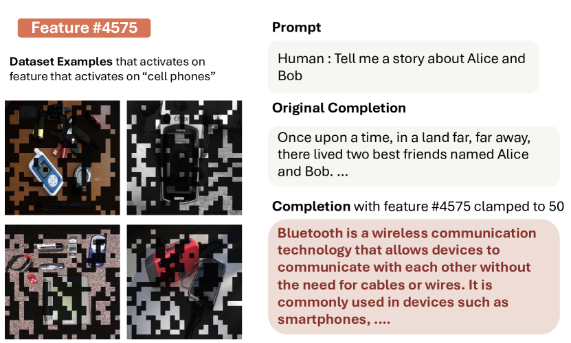
Figure 18: The feature related to money and its steering effect.

11 Feature Probing

Due to the large number of features, identifying specific features of interest is challenging, and interpreting all available features before making a selection is impractical. Following Templeton et al. [35], we also probe into the features of our SAE to identify several emotion-related features that may influence the model’s perceived emotional responses. We first prepare an image representing a specific emotion, then select the top-k activated features for that image to run through our explanation and steering pipeline. From the output, we manually select the desired features and validate them through steering and activated examples. Unlike the approach in [35], which uses only the top 5 activated features, we found that a higher value of $k$ is preferable because a single image can contain many low-level visual features and diverse semantic information. In practice, we select $30\leq k\leq 100$ and skip some of the top-activated values to exclude low-level visual features.

12 Low Level Perception Features Examples

We identify many low-level visual features from the model that differ from the text-based features in large language models (LLMs). These visual features are strongly activated across most images and represent the model’s basic perceptual and cognitive abilities. In Fig. 17, we present examples of features activated by structure, shape, and color. In many of our probing trials, these features exhibit high activation levels and respond to various aspects of the images. We believe these features function as universal elements in how language-vision models (LMMs) understand the world.

References

- Agarwal et al. [2014] Alekh Agarwal, Animashree Anandkumar, Prateek Jain, and Praneeth Netrapalli. Learning sparsely used overcomplete dictionaries via alternating minimization, 2014.
- Apple [2024] Apple. Apple intelligence is available today on iphone, ipad and mac. https://www.apple.com/sg/newsroom/2024/10/apple-intelligence-is-available-today-on-iphone-ipad-and-mac/, 2024.
- Bai et al. [2023] Jinze Bai, Shuai Bai, Shusheng Yang, Shijie Wang, Sinan Tan, Peng Wang, Junyang Lin, Chang Zhou, and Jingren Zhou. Qwen-vl: A versatile vision-language model for understanding, localization, text reading, and beyond. arXiv preprint arXiv:2308.12966, 2023.
- Bau et al. [2017] David Bau, Bolei Zhou, Aditya Khosla, Aude Oliva, and Antonio Torralba. Network dissection: Quantifying interpretability of deep visual representations. In Proceedings of the IEEE conference on computer vision and pattern recognition, pages 6541–6549, 2017.
- Bills et al. [2023] Steven Bills, Nick Cammarata, Dan Mossing, Henk Tillman, Leo Gao, Gabriel Goh, Ilya Sutskever, Jan Leike, Jeff Wu, and William Saunders. Language models can explain neurons in language models. https://openaipublic.blob.core.windows.net/neuron-explainer/paper/index.html, 2023.
- Bricken et al. [2023] Trenton Bricken, Adly Templeton, Joshua Batson, Brian Chen, Adam Jermyn, Tom Conerly, Nick Turner, Cem Anil, Carson Denison, Amanda Askell, Robert Lasenby, Yifan Wu, Shauna Kravec, Nicholas Schiefer, Tim Maxwell, Nicholas Joseph, Zac Hatfield-Dodds, Alex Tamkin, Karina Nguyen, Brayden McLean, Josiah E Burke, Tristan Hume, Shan Carter, Tom Henighan, and Christopher Olah. Towards monosemanticity: Decomposing language models with dictionary learning. Transformer Circuits Thread, 2023. https://transformer-circuits.pub/2023/monosemantic-features/index.html.
- Chen et al. [2024a] Shuo Chen, Zhen Han, Bailan He, Zifeng Ding, Wenqian Yu, Philip Torr, Volker Tresp, and Jindong Gu. Red teaming gpt-4v: Are gpt-4v safe against uni/multi-modal jailbreak attacks?, 2024a.
- Chen et al. [2024b] Zhe Chen, Jiannan Wu, Wenhai Wang, Weijie Su, Guo Chen, Sen Xing, Muyan Zhong, Qinglong Zhang, Xizhou Zhu, Lewei Lu, et al. Internvl: Scaling up vision foundation models and aligning for generic visual-linguistic tasks. In Proceedings of the IEEE/CVF Conference on Computer Vision and Pattern Recognition, pages 24185–24198, 2024b.
- Dubey et al. [2024] Abhimanyu Dubey, Abhinav Jauhri, Abhinav Pandey, Abhishek Kadian, Ahmad Al-Dahle, Aiesha Letman, Akhil Mathur, Alan Schelten, Amy Yang, Angela Fan, Anirudh Goyal, Anthony Hartshorn, Aobo Yang, Archi Mitra, Archie Sravankumar, Artem Korenev, Arthur Hinsvark, Arun Rao, Aston Zhang, Aurelien Rodriguez, Austen Gregerson, Ava Spataru, Baptiste Roziere, Bethany Biron, Binh Tang, Bobbie Chern, Charlotte Caucheteux, Chaya Nayak, Chloe Bi, Chris Marra, Chris McConnell, Christian Keller, Christophe Touret, Chunyang Wu, Corinne Wong, Cristian Canton Ferrer, Cyrus Nikolaidis, Damien Allonsius, Daniel Song, Danielle Pintz, Danny Livshits, David Esiobu, Dhruv Choudhary, Dhruv Mahajan, Diego Garcia-Olano, Diego Perino, Dieuwke Hupkes, Egor Lakomkin, Ehab AlBadawy, Elina Lobanova, Emily Dinan, Eric Michael Smith, Filip Radenovic, Frank Zhang, Gabriel Synnaeve, Gabrielle Lee, Georgia Lewis Anderson, Graeme Nail, Gregoire Mialon, Guan Pang, Guillem Cucurell, Hailey Nguyen, Hannah Korevaar, Hu Xu, Hugo Touvron, Iliyan Zarov, Imanol Arrieta Ibarra, Isabel Kloumann, Ishan Misra, Ivan Evtimov, Jade Copet, Jaewon Lee, Jan Geffert, Jana Vranes, Jason Park, Jay Mahadeokar, Jeet Shah, Jelmer van der Linde, Jennifer Billock, Jenny Hong, Jenya Lee, Jeremy Fu, Jianfeng Chi, Jianyu Huang, Jiawen Liu, Jie Wang, Jiecao Yu, Joanna Bitton, Joe Spisak, Jongsoo Park, Joseph Rocca, Joshua Johnstun, Joshua Saxe, Junteng Jia, Kalyan Vasuden Alwala, Kartikeya Upasani, Kate Plawiak, Ke Li, Kenneth Heafield, Kevin Stone, Khalid El-Arini, Krithika Iyer, Kshitiz Malik, Kuenley Chiu, Kunal Bhalla, Lauren Rantala-Yeary, Laurens van der Maaten, Lawrence Chen, Liang Tan, Liz Jenkins, Louis Martin, Lovish Madaan, Lubo Malo, Lukas Blecher, Lukas Landzaat, Luke de Oliveira, Madeline Muzzi, Mahesh Pasupuleti, Mannat Singh, Manohar Paluri, Marcin Kardas, Mathew Oldham, Mathieu Rita, Maya Pavlova, Melanie Kambadur, Mike Lewis, Min Si, Mitesh Kumar Singh, Mona Hassan, Naman Goyal, Narjes Torabi, Nikolay Bashlykov, Nikolay Bogoychev, Niladri Chatterji, Olivier Duchenne, Onur Çelebi, Patrick Alrassy, Pengchuan Zhang, Pengwei Li, Petar Vasic, Peter Weng, Prajjwal Bhargava, Pratik Dubal, Praveen Krishnan, Punit Singh Koura, Puxin Xu, Qing He, Qingxiao Dong, Ragavan Srinivasan, Raj Ganapathy, Ramon Calderer, Ricardo Silveira Cabral, Robert Stojnic, Roberta Raileanu, Rohit Girdhar, Rohit Patel, Romain Sauvestre, Ronnie Polidoro, Roshan Sumbaly, Ross Taylor, Ruan Silva, Rui Hou, Rui Wang, Saghar Hosseini, Sahana Chennabasappa, Sanjay Singh, Sean Bell, Seohyun Sonia Kim, Sergey Edunov, Shaoliang Nie, Sharan Narang, Sharath Raparthy, Sheng Shen, Shengye Wan, Shruti Bhosale, Shun Zhang, Simon Vandenhende, Soumya Batra, Spencer Whitman, Sten Sootla, Stephane Collot, Suchin Gururangan, Sydney Borodinsky, Tamar Herman, Tara Fowler, Tarek Sheasha, Thomas Georgiou, Thomas Scialom, Tobias Speckbacher, Todor Mihaylov, Tong Xiao, Ujjwal Karn, Vedanuj Goswami, Vibhor Gupta, Vignesh Ramanathan, Viktor Kerkez, Vincent Gonguet, Virginie Do, Vish Vogeti, Vladan Petrovic, Weiwei Chu, Wenhan Xiong, Wenyin Fu, Whitney Meers, Xavier Martinet, Xiaodong Wang, Xiaoqing Ellen Tan, Xinfeng Xie, Xuchao Jia, Xuewei Wang, Yaelle Goldschlag, Yashesh Gaur, Yasmine Babaei, Yi Wen, Yiwen Song, Yuchen Zhang, Yue Li, Yuning Mao, Zacharie Delpierre Coudert, Zheng Yan, Zhengxing Chen, Zoe Papakipos, Aaditya Singh, Aaron Grattafiori, Abha Jain, Adam Kelsey, Adam Shajnfeld, Adithya Gangidi, Adolfo Victoria, Ahuva Goldstand, Ajay Menon, Ajay Sharma, Alex Boesenberg, Alex Vaughan, Alexei Baevski, Allie Feinstein, Amanda Kallet, Amit Sangani, Anam Yunus, Andrei Lupu, Andres Alvarado, Andrew Caples, Andrew Gu, Andrew Ho, Andrew Poulton, Andrew Ryan, Ankit Ramchandani, Annie Franco, Aparajita Saraf, Arkabandhu Chowdhury, Ashley Gabriel, Ashwin Bharambe, Assaf Eisenman, Azadeh Yazdan, Beau James, Ben Maurer, Benjamin Leonhardi, Bernie Huang, Beth Loyd, Beto De Paola, Bhargavi Paranjape, Bing Liu, Bo Wu, Boyu Ni, Braden Hancock, Bram Wasti, Brandon Spence, Brani Stojkovic, Brian Gamido, Britt Montalvo, Carl Parker, Carly Burton, Catalina Mejia, Changhan Wang, Changkyu Kim, Chao Zhou, Chester Hu, Ching-Hsiang Chu, Chris Cai, Chris Tindal, Christoph Feichtenhofer, Damon Civin, Dana Beaty, Daniel Kreymer, Daniel Li, Danny Wyatt, David Adkins, David Xu, Davide Testuggine, Delia David, Devi Parikh, Diana Liskovich, Didem Foss, Dingkang Wang, Duc Le, Dustin Holland, Edward Dowling, Eissa Jamil, Elaine Montgomery, Eleonora Presani, Emily Hahn, Emily Wood, Erik Brinkman, Esteban Arcaute, Evan Dunbar, Evan Smothers, Fei Sun, Felix Kreuk, Feng Tian, Firat Ozgenel, Francesco Caggioni, Francisco Guzmán, Frank Kanayet, Frank Seide, Gabriela Medina Florez, Gabriella Schwarz, Gada Badeer, Georgia Swee, Gil Halpern, Govind Thattai, Grant Herman, Grigory Sizov, Guangyi, Zhang, Guna Lakshminarayanan, Hamid Shojanazeri, Han Zou, Hannah Wang, Hanwen Zha, Haroun Habeeb, Harrison Rudolph, Helen Suk, Henry Aspegren, Hunter Goldman, Ibrahim Damlaj, Igor Molybog, Igor Tufanov, Irina-Elena Veliche, Itai Gat, Jake Weissman, James Geboski, James Kohli, Japhet Asher, Jean-Baptiste Gaya, Jeff Marcus, Jeff Tang, Jennifer Chan, Jenny Zhen, Jeremy Reizenstein, Jeremy Teboul, Jessica Zhong, Jian Jin, Jingyi Yang, Joe Cummings, Jon Carvill, Jon Shepard, Jonathan McPhie, Jonathan Torres, Josh Ginsburg, Junjie Wang, Kai Wu, Kam Hou U, Karan Saxena, Karthik Prasad, Kartikay Khandelwal, Katayoun Zand, Kathy Matosich, Kaushik Veeraraghavan, Kelly Michelena, Keqian Li, Kun Huang, Kunal Chawla, Kushal Lakhotia, Kyle Huang, Lailin Chen, Lakshya Garg, Lavender A, Leandro Silva, Lee Bell, Lei Zhang, Liangpeng Guo, Licheng Yu, Liron Moshkovich, Luca Wehrstedt, Madian Khabsa, Manav Avalani, Manish Bhatt, Maria Tsimpoukelli, Martynas Mankus, Matan Hasson, Matthew Lennie, Matthias Reso, Maxim Groshev, Maxim Naumov, Maya Lathi, Meghan Keneally, Michael L. Seltzer, Michal Valko, Michelle Restrepo, Mihir Patel, Mik Vyatskov, Mikayel Samvelyan, Mike Clark, Mike Macey, Mike Wang, Miquel Jubert Hermoso, Mo Metanat, Mohammad Rastegari, Munish Bansal, Nandhini Santhanam, Natascha Parks, Natasha White, Navyata Bawa, Nayan Singhal, Nick Egebo, Nicolas Usunier, Nikolay Pavlovich Laptev, Ning Dong, Ning Zhang, Norman Cheng, Oleg Chernoguz, Olivia Hart, Omkar Salpekar, Ozlem Kalinli, Parkin Kent, Parth Parekh, Paul Saab, Pavan Balaji, Pedro Rittner, Philip Bontrager, Pierre Roux, Piotr Dollar, Polina Zvyagina, Prashant Ratanchandani, Pritish Yuvraj, Qian Liang, Rachad Alao, Rachel Rodriguez, Rafi Ayub, Raghotham Murthy, Raghu Nayani, Rahul Mitra, Raymond Li, Rebekkah Hogan, Robin Battey, Rocky Wang, Rohan Maheswari, Russ Howes, Ruty Rinott, Sai Jayesh Bondu, Samyak Datta, Sara Chugh, Sara Hunt, Sargun Dhillon, Sasha Sidorov, Satadru Pan, Saurabh Verma, Seiji Yamamoto, Sharadh Ramaswamy, Shaun Lindsay, Shaun Lindsay, Sheng Feng, Shenghao Lin, Shengxin Cindy Zha, Shiva Shankar, Shuqiang Zhang, Shuqiang Zhang, Sinong Wang, Sneha Agarwal, Soji Sajuyigbe, Soumith Chintala, Stephanie Max, Stephen Chen, Steve Kehoe, Steve Satterfield, Sudarshan Govindaprasad, Sumit Gupta, Sungmin Cho, Sunny Virk, Suraj Subramanian, Sy Choudhury, Sydney Goldman, Tal Remez, Tamar Glaser, Tamara Best, Thilo Kohler, Thomas Robinson, Tianhe Li, Tianjun Zhang, Tim Matthews, Timothy Chou, Tzook Shaked, Varun Vontimitta, Victoria Ajayi, Victoria Montanez, Vijai Mohan, Vinay Satish Kumar, Vishal Mangla, Vítor Albiero, Vlad Ionescu, Vlad Poenaru, Vlad Tiberiu Mihailescu, Vladimir Ivanov, Wei Li, Wenchen Wang, Wenwen Jiang, Wes Bouaziz, Will Constable, Xiaocheng Tang, Xiaofang Wang, Xiaojian Wu, Xiaolan Wang, Xide Xia, Xilun Wu, Xinbo Gao, Yanjun Chen, Ye Hu, Ye Jia, Ye Qi, Yenda Li, Yilin Zhang, Ying Zhang, Yossi Adi, Youngjin Nam, Yu, Wang, Yuchen Hao, Yundi Qian, Yuzi He, Zach Rait, Zachary DeVito, Zef Rosnbrick, Zhaoduo Wen, Zhenyu Yang, and Zhiwei Zhao. The llama 3 herd of models, 2024.
- Elad [2010] Michael Elad. Sparse and redundant representations: from theory to applications in signal and image processing. Springer Science & Business Media, 2010.
- Elhage et al. [2022] Nelson Elhage, Tristan Hume, Catherine Olsson, Nicholas Schiefer, Tom Henighan, Shauna Kravec, Zac Hatfield-Dodds, Robert Lasenby, Dawn Drain, Carol Chen, et al. Toy models of superposition. arXiv preprint arXiv:2209.10652, 2022.
- Fu et al. [2024] Chaoyou Fu, Peixian Chen, Yunhang Shen, Yulei Qin, Mengdan Zhang, Xu Lin, Jinrui Yang, Xiawu Zheng, Ke Li, Xing Sun, Yunsheng Wu, and Rongrong Ji. Mme: A comprehensive evaluation benchmark for multimodal large language models, 2024.
- Gao et al. [2024] Leo Gao, Tom Dupré la Tour, Henk Tillman, Gabriel Goh, Rajan Troll, Alec Radford, Ilya Sutskever, Jan Leike, and Jeffrey Wu. Scaling and evaluating sparse autoencoders, 2024.
- Guan et al. [2023] Tianrui Guan, Fuxiao Liu, Xiyang Wu, Ruiqi Xian, Zongxia Li, Xiaoyu Liu, Xijun Wang, Lichang Chen, Furong Huang, Yaser Yacoob, Dinesh Manocha, and Tianyi Zhou. Hallusionbench: An advanced diagnostic suite for entangled language hallucination & visual illusion in large vision-language models, 2023.
- Kirillov et al. [2023] Alexander Kirillov, Eric Mintun, Nikhila Ravi, Hanzi Mao, Chloe Rolland, Laura Gustafson, Tete Xiao, Spencer Whitehead, Alexander C. Berg, Wan-Yen Lo, Piotr Dollár, and Ross Girshick. Segment anything. arXiv:2304.02643, 2023.
- Li et al. [2024a] Bo Li, Kaichen Zhang, Hao Zhang, Dong Guo, Renrui Zhang, Feng Li, Yuanhan Zhang, Ziwei Liu, and Chunyuan Li. Llava-next: Stronger llms supercharge multimodal capabilities in the wild, 2024a.
- Li et al. [2024b] Bo Li, Yuanhan Zhang, Dong Guo, Renrui Zhang, Feng Li, Hao Zhang, Kaichen Zhang, Peiyuan Zhang, Yanwei Li, Ziwei Liu, and Chunyuan Li. Llava-onevision: Easy visual task transfer, 2024b.
- Lieberum et al. [2024] Tom Lieberum, Senthooran Rajamanoharan, Arthur Conmy, Lewis Smith, Nicolas Sonnerat, Vikrant Varma, János Kramár, Anca Dragan, Rohin Shah, and Neel Nanda. Gemma scope: Open sparse autoencoders everywhere all at once on gemma 2, 2024.
- Lin et al. [2015] Tsung-Yi Lin, Michael Maire, Serge Belongie, Lubomir Bourdev, Ross Girshick, James Hays, Pietro Perona, Deva Ramanan, C. Lawrence Zitnick, and Piotr Dollár. Microsoft coco: Common objects in context, 2015.
- Liu et al. [2024a] Haotian Liu, Chunyuan Li, Yuheng Li, Bo Li, Yuanhan Zhang, Sheng Shen, and Yong Jae Lee. Llava-next: Improved reasoning, ocr, and world knowledge, 2024a.
- Liu et al. [2024b] Haotian Liu, Chunyuan Li, Qingyang Wu, and Yong Jae Lee. Visual instruction tuning. Advances in neural information processing systems, 36, 2024b.
- Liu et al. [2023] Shilong Liu, Zhaoyang Zeng, Tianhe Ren, Feng Li, Hao Zhang, Jie Yang, Chunyuan Li, Jianwei Yang, Hang Su, Jun Zhu, et al. Grounding dino: Marrying dino with grounded pre-training for open-set object detection. arXiv preprint arXiv:2303.05499, 2023.
- Liu et al. [2024c] Sheng Liu, Haotian Ye, and James Zou. Reducing hallucinations in vision-language models via latent space steering. arXiv preprint arXiv:2410.15778, 2024c.
- Ma et al. [2024] Yueen Ma, Zixing Song, Yuzheng Zhuang, Jianye Hao, and Irwin King. A survey on vision-language-action models for embodied ai. arXiv preprint arXiv:2405.14093, 2024.
- Makhzani and Frey [2014] Alireza Makhzani and Brendan Frey. k-sparse autoencoders, 2014.
- Meta [2024] Meta. Introducing orion: Our first true augmented reality glasses. https://about.fb.com/news/2024/09/introducing-orion-our-first-true-augmented-reality-glasses/, 2024.
- Nanda [2023] Neel Nanda. Attribution patching: Activation patching at industrial scale. https://www.neelnanda.io/mechanistic-interpretability/attribution-patching, 2023. Accessed: 2024-09-30.
- Olah et al. [2017] Chris Olah, Alexander Mordvintsev, and Ludwig Schubert. Feature visualization. Distill, 2017. https://distill.pub/2017/feature-visualization.
- Olah et al. [2020] Chris Olah, Nick Cammarata, Ludwig Schubert, Gabriel Goh, Michael Petrov, and Shan Carter. Zoom in: An introduction to circuits. Distill, 5(3):e00024–001, 2020.
- Olshausen and Field [1996] Bruno A Olshausen and David J Field. Emergence of simple-cell receptive field properties by learning a sparse code for natural images. Nature, 381(6583):607–609, 1996.
- Parekh et al. [2024] Jayneel Parekh, Pegah Khayatan, Mustafa Shukor, Alasdair Newson, and Matthieu Cord. A concept-based explainability framework for large multimodal models, 2024.
- Quiroga et al. [2005] R Quian Quiroga, Leila Reddy, Gabriel Kreiman, Christof Koch, and Itzhak Fried. Invariant visual representation by single neurons in the human brain. Nature, 435(7045):1102–1107, 2005.
- Schaeffer et al. [2024] Rylan Schaeffer, Dan Valentine, Luke Bailey, James Chua, Cristóbal Eyzaguirre, Zane Durante, Joe Benton, Brando Miranda, Henry Sleight, John Hughes, Rajashree Agrawal, Mrinank Sharma, Scott Emmons, Sanmi Koyejo, and Ethan Perez. When do universal image jailbreaks transfer between vision-language models?, 2024.
- Shen and Zhou [2021] Yujun Shen and Bolei Zhou. Closed-form factorization of latent semantics in gans. In Proceedings of the IEEE/CVF conference on computer vision and pattern recognition, pages 1532–1540, 2021.
- Templeton et al. [2024] Adly Templeton, Tom Conerly, Jonathan Marcus, Jack Lindsey, Trenton Bricken, Brian Chen, Adam Pearce, Craig Citro, Emmanuel Ameisen, Andy Jones, Hoagy Cunningham, Nicholas L Turner, Callum McDougall, Monte MacDiarmid, C. Daniel Freeman, Theodore R. Sumers, Edward Rees, Joshua Batson, Adam Jermyn, Shan Carter, Chris Olah, and Tom Henighan. Scaling monosemanticity: Extracting interpretable features from claude 3 sonnet. Transformer Circuits Thread, 2024.
- Tong et al. [2024] Shengbang Tong, Ellis Brown, Penghao Wu, Sanghyun Woo, Manoj Middepogu, Sai Charitha Akula, Jihan Yang, Shusheng Yang, Adithya Iyer, Xichen Pan, Austin Wang, Rob Fergus, Yann LeCun, and Saining Xie. Cambrian-1: A fully open, vision-centric exploration of multimodal llms, 2024.
- Wang et al. [2022] Kevin Wang, Alexandre Variengien, Arthur Conmy, Buck Shlegeris, and Jacob Steinhardt. Interpretability in the wild: a circuit for indirect object identification in gpt-2 small, 2022.
- Wang et al. [2024] Peng Wang, Shuai Bai, Sinan Tan, Shijie Wang, Zhihao Fan, Jinze Bai, Keqin Chen, Xuejing Liu, Jialin Wang, Wenbin Ge, Yang Fan, Kai Dang, Mengfei Du, Xuancheng Ren, Rui Men, Dayiheng Liu, Chang Zhou, Jingren Zhou, and Junyang Lin. Qwen2-vl: Enhancing vision-language model’s perception of the world at any resolution, 2024.
- Yang et al. [2023] Zhengyuan Yang, Linjie Li, Kevin Lin, Jianfeng Wang, Chung-Ching Lin, Zicheng Liu, and Lijuan Wang. The dawn of lmms: Preliminary explorations with gpt-4v (ision). arXiv preprint arXiv:2309.17421, 9(1):1, 2023.
- Yu et al. [2023] Weihao Yu, Zhengyuan Yang, Linjie Li, Jianfeng Wang, Kevin Lin, Zicheng Liu, Xinchao Wang, and Lijuan Wang. Mm-vet: Evaluating large multimodal models for integrated capabilities, 2023.
- Zheng et al. [2024] Lianmin Zheng, Liangsheng Yin, Zhiqiang Xie, Chuyue Sun, Jeff Huang, Cody Hao Yu, Shiyi Cao, Christos Kozyrakis, Ion Stoica, Joseph E. Gonzalez, Clark Barrett, and Ying Sheng. Sglang: Efficient execution of structured language model programs, 2024.
- Zhou et al. [2014] Bolei Zhou, Aditya Khosla, Agata Lapedriza, Aude Oliva, and Antonio Torralba. Object detectors emerge in deep scene cnns. arXiv preprint arXiv:1412.6856, 2014.