Generalized Multivariate Polynomial Codes for Distributed Matrix-Matrix Multiplication

Abstract

Supporting multiple partial computations efficiently at each of the workers is a keystone in distributed coded computing in order to speed up computations and to fully exploit the resources of heterogeneous workers in terms of communication, storage, or computation capabilities. Multivariate polynomial coding schemes have recently been shown to deliver faster results for distributed matrix-matrix multiplication compared to conventional univariate polynomial coding schemes by supporting multiple partial coded computations at each worker at reduced communication costs. In this work, we extend multivariate coding schemes to also support arbitrary matrix partitions. Generalized matrix partitions have been proved useful to trade-off between computation speed and communication costs in distributed (univariate) coded computing. We first formulate the computation latency-communication trade-off in terms of the computation complexity and communication overheads required by coded computing approaches as compared to a single server uncoded computing system. Then, we propose two novel multivariate coded computing schemes supporting arbitrary matrix partitions. The proposed schemes are shown to improve the studied trade-off as compared to univariate schemes.

I Introduction

Matrix-matrix multiplication is a fundamental operation that arises in many problems, particularly in emerging machine learning applications. When the input matrices are from large datasetscomputing matrix multiplications on a single server within a reasonable amount of time becomes unfeasible. It is thus essential to split the job into multiple subtasks and execute them on multiple servers in parallel. However, servers in modern large distributed computation clusters usually comprise small, low-end, and unreliable computational nodes which are severely affected by “system noise”, i.e., faulty behaviors due to computation or memory bottlenecks, load imbalance, resource contention, hardware issues, etc [1]. As a result, task completion times of individual workers become largely unpredictable, and the slowest workers dominate the overall computation time. This is referred to in the literature as the straggler problem.

In this work, we address this problem by adopting the coded computing framework initiated in [2, 3, 4, 5]. A formulation based on maximum distance separable (MDS) codes was first presented in [2]. In coded computing, unlike conventional schemes that rely on subtask repetition, any delayed subtask can be replaced by any other subtask. As a result, coded-computing-based solutions provide order-wise improvements in task completion times. In particular, it was possible to recover the original matrix-matrix product from a number of computations, referred to as recovery threshold that did not increase with the number of workers, but rather with the total number of matrix block products. Univariate polynomial codes, a form of MDS codes with a particularly efficient decoding procedure via polynomial interpolation, were described, simultaneously, in [5] referred to as entangled polynomial codes, and in [6] referred to as generalized PolyDot codes. These schemes offered flexibility to trade the computation complexity for download communications resources. Follow-up works extended the results to secure matrix-matrix multiplications [7, 8], matrix chain multiplications[9], among others.

All these works consider a distributed computation model in which a single subtask is assigned to each worker. To further speed up computations and to better support heterogeneous workers, subsequent works [10, 11, 12, 13, 14] consider instead a distributed computation model with multiple subtasks per worker. By assigning multiple, smaller subtasks to workers it can be shown that any partial work conducted by straggler workers can also be exploited. In [15, 16] it was shown that univariate polynomial coding schemes are inefficient in terms of the upload communication costs, i.e., the resources needed to communicate the coded matrices from the master server to workers. To address this inefficiency, bivariate polynomial codes are proposed in [16]. These schemes, however, cannot support generalized partition schemes, failing to trade computation complexity with the download communication cost.

In this work, we provide an extension of the bivariate codes proposed in [16] to accommodate generalized matrix partitions. We introduce two novel multivariate schemes achieving new points in the trade-off curves between the computation complexity and upload/download communication overheads.

The remainder of the paper is organized as follows. In Section II, the problem formulation is presented. Section III characterizes the univariate polynomial coding scheme. Next, Section IV introduces the proposed multivariate polynomial codes. Numerical results are provided in Section V. Finally, conclusions are drawn in Section VI.

II System Model and Problem Formulation

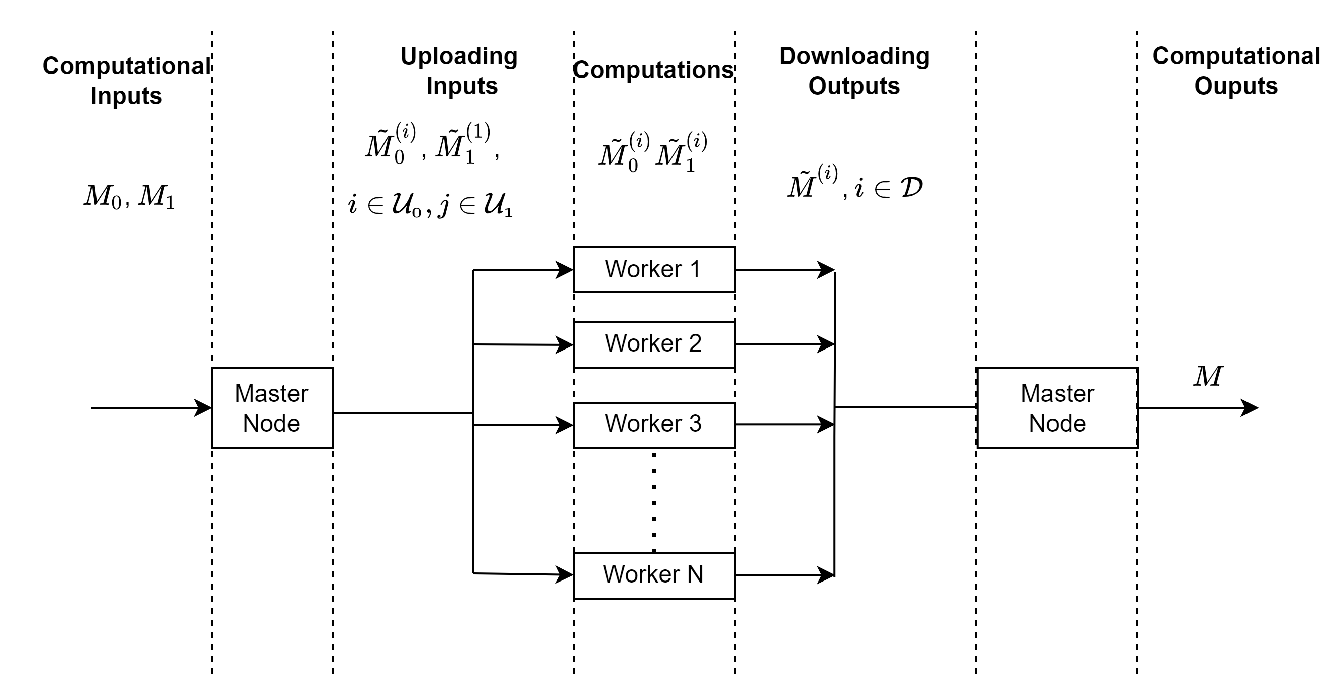
Figure 1: Distributed computational system.

We consider the problem of outsourcing the task of multiplying two large matrices $M_{0}\in\mathbb{F}^{r_{0}\times r_{1}}$ and $M_{1}\in\mathbb{F}^{r_{1}\times r_{2}}$ from a centralized master node to a more computational powerful entity with $N$ parallel computation nodes/workers, see Figure 1. For that, the master node splits the task into several subtasks and sends (uploads) appropriate, eg. coded subtask inputs to the nodes. These nodes in parallel and under a timely coordination from the master, compute distinct subtasks, and send the results back (downloaded) to the master node. Multiple subtasks can be assigned to each worker, in which case, these subtasks are executed sequentially. By exploiting task partitions and distributing the computation between workers, the overall computation time can be reduced. However, as we will show in this work, there is a computation complexity and communication overhead associated to task partitioning. For the uplink communication from the master to the workers, we assume that each subtask input can be broadcasted to all the workers at the cost of transmitting only one subtask, i.e. wireless broadcast model. Workers coordinated by the master, store or discard the subtask inputs received. For the downlink, each computation output makes use of separate resources.

Specifically, in order to distribute the total computation work, matrix $M_{0}$ is partitioned into $p_{0}$ partitions vertically and $p_{1}$ partitions horizontally, resulting in $p_{0}p_{1}$ matrix block partitions $M_{0}^{b_{0},b_{1}}\in\mathbb{F}^{\frac{r_{0}}{p_{0}}\times\frac{r_{1}}{p_{1}}}$, for $b_{0}\in\left[p_{0}\right]$ and $b_{1}\in\left[p_{1}\right]$ where we denoted $\left[n\right]=\left\{0,1,\dots,n-1\right\}$. Similarly, matrix $M_{1}$ is partitioned into $p_{1}$ partitions vertically, and $p_{2}$ partitions horizontally, resulting in $p_{1}p_{2}$ matrix block partitions $M_{1}^{b_{1},b_{2}}\in\mathbb{F}^{\frac{r_{1}}{p_{1}}\times\frac{r_{2}}{p_{2}}}$ for $b_{1}\in\left[p_{1}\right]$ and $b_{2}\in\left[p_{2}\right]$, i.e.,

$$M_{i} = \left[\begin{array}[]{ccc}M_{i}^{0,0}&\cdots&M_{i}^{0,p_{i+1}-1}\\ \vdots&\ddots&\vdots\\ M_{i}^{p_{i}-1,0}&\cdots&M_{i}^{p_{i}-1,p_{i+1}-1}\end{array}\right]$$

for $i\in\left\{0,1\right\}$. The result of the multiplication of $M_{0}$ and $M_{1}$, as a function of its matrix blocks, can be written as

$$M=M_{0}M_{1} = \left[\begin{array}[]{ccc}M^{0,0}&\cdots&M^{0,p_{2}-1}\\ \vdots&\ddots&\vdots\\ M^{p_{0}-1,0}&\cdots&M^{p_{0}-1,p_{2}-1}\end{array}\right]$$ (5)

with $M^{n_{0},n_{2}}=\sum_{n_{1}=0}^{p_{1}-1}M^{n_{0},n_{1}}M_{1}^{n_{1},n_{2}}$. From (5) we can readily see that $M$ is comprised of $p_{0}p_{2}$ matrix block partitions. Given that each matrix block partition involves $p_{1}$ matrix-matrix multiplications, a total of $K=p_{0}p_{1}p_{2}$ different block matrix-matrix multiplications $M_{0}^{n_{0},n_{1}}M_{1}^{n_{1},n_{2}}$ $\left(n_{0},n_{1},n_{2}\right)\in\left[p_{0}\right]\times\left[p_{1}\right]\times\left[p_{2}\right]$ are needed to recover the original multiplication. We refer to the triplet $\left(p_{0},p_{1},p_{2}\right)$ as the partition scheme and $K$ as the partition level.

Given these matrix partitions, an uncoded distributed computation scheme consists of distributing each of these block matrix-matrix multiplications into the different parallel workers. However, any delay in one of these computations, results in a delay in the overall computation. This is known as the straggler problem in distributed computing. A straightforward solution, although inefficient, is work repetition, i.e., replicating each of the block matrix-matrix products into different workers. Since every replicated computation can only replace one specific block multiplication, the number of workers needed grows linearly with the partition level. Coded computing offers a much more efficient approach to this problem. At the master server, block matrices from $M_{0}$ are linearly encoded into $\left|\mathcal{U}_{0}\right|$ coded block matrices, i.e., $\tilde{M}_{0}^{(i)}\in\mathbb{F}^{\frac{r_{0}}{p_{0}}\times\frac{r_{1}}{p_{1}}}$, $i\in\mathcal{U}_{0}$, and, similarly, block matrices from $M_{1}$ are linearly encoded into $\left|\mathcal{U}_{1}\right|$ coded block matrices, i.e., $\tilde{M}_{1}^{(i)}\in\mathbb{F}^{\frac{r_{1}}{p_{1}}\times\frac{r_{2}}{p_{2}}},$$i\in\left|\mathcal{U}_{1}\right|$. Then, coded block matrices from $M_{0}$ and $M_{1}$ are distributed to the $N$ workers in the system, which then compute the coded block matrix-matrix multiplications $\tilde{M}^{(i)}=\tilde{M}_{0}^{(i)}\tilde{M}_{1}^{(i)}\in\mathbb{F}^{\frac{r_{0}}{p_{0}}\times\frac{r_{2}}{p_{2}}}$, each of which is referred to as a subtask. In order to exploit partial work, we also consider that each worker may compute multiple subtasks in a serial manner. That is, as soon as a worker finishes a subtask, it returns the result to the master for decoding and proceeds to compute another subtask. After receiving a number of computations known as the recovery threshold, $R_{th}$, the master is able to decode the target matrix-matrix multiplication, $M_{0}M_{1}$. In contrast to work repetition, in coded computing, any computation can be replaced by another that could have been delayed.

TABLE I: Computation complexity and upload/download communications overheads for different coded distributed computing methods

Method∗	$R_{th}$	$\delta$	$\delta_{u,0}$	$\delta_{u,1}$	$\delta_{d}$
epc	$p_{1}p_{2}p_{0}+p_{1}-1$	$\frac{p_{1}-1}{p_{0}p_{1}p_{2}}$	$p_{2}-1+p_{2}\delta$	$p_{0}-1+p_{0}\delta$	$p_{1}-1+p_{1}\delta$
Bi0	$p_{0}p_{2}p_{1}+p_{0}\left(p_{1}-1\right)$	$\frac{p_{1}-1}{p_{0}p_{1}}$	$\delta$	$p_{0}-1+p_{0}\delta$	$p_{1}-1+p_{1}\delta$
Bi2	$p_{0}p_{1}p_{2}+p_{2}\left(p_{1}-1\right)$	$\frac{p_{1}-1}{p_{1}p_{2}}$	$p_{2}-1+p_{2}\delta$	$\delta$	$p_{1}-1+p_{1}\delta$
Tri	$p_{0}p_{2}p_{1}+p_{0}p_{2}\left(p_{1}-1\right)$	$\frac{p_{1}-1}{p_{1}}$	$\delta$	$\delta$	$p_{1}-1+p_{1}\delta$

^∗See Section III and IV for the definition of these abreviations.

Although coded computing is an efficient method to achieve lower computation latencies, it incurs communication and computation complexity overheads. The average computation latency is here defined as the average time taken to obtain the computation result. For simplicity, we assume the computation latency is mainly dominated by the computation time at workers. We get lower computation latency as we increase the number of parallel workers, $N$, since there is more work parallelization, but also as we increase the partition level, $K$, since then each subtask becomes smaller and less work is left unfinished at the workers by the time $R_{th}$ computations are completed.

For the overheads, we will use as a reference, the setting where we outsource the computation to a single server, which we refer to as SS. Then, we define the computation complexity overhead, $\delta$, as the increment in computation complexity, i.e., number of element-wise multiplications, required by coded computing $C^{\text{CC}}$, relative to the computation complexity in a single server, $C^{\text{SS}}$. That is, $C^{\text{CC}}=C^{\text{SS}}\left(1+\delta\right)$. For the uncoded single server setting, multiplication involves, roughly, $C^{\text{SS}}=r_{0}r_{1}r_{2}$ element-wise multiplications . Likewise, for coded computing, each partial computation at the workers involves $\frac{r_{0}}{p_{0}}\frac{r_{1}}{p_{1}}\frac{r_{2}}{p_{1}}$ element-wise multiplications. Given that $R_{th}$ subtasks are required, the computation complexity is $C^{\text{CC}}=R_{th}\frac{r_{0}}{p_{0}}\frac{r_{1}}{p_{1}}\frac{r_{2}}{p_{1}}$, and thus the computation overheads is

$$\delta = \frac{C^{\text{CC}}}{C^{\text{SS}}}-1=\frac{R_{th}}{K}-1.$$ (6)

The download communication overhead, $\delta_{d}$, is similarly defined as the increment of the cost of communicating the block matrix products from the workers to the master in coded computing, $C_{d}^{\text{CC}}$, relative to the cost of communicating the original product result from a single server, $C_{d}^{\text{SS}}$. That is $C_{d}^{\text{CC}}=C_{d}^{\text{SS}}\left(1+\delta_{d}\right)$. If we measure the communication cost in units of the size of the entries of the resultant product matrix, we have that, since $R_{th}$ block matrix products, i.e., subtasks, are returned, each of size $\frac{r_{0}}{p_{0}}\frac{r_{2}}{p_{2}}$, the cost is $C_{d}^{\text{CC}}=R_{th}\frac{r_{0}r_{2}}{p_{0}p_{2}}$. On the other hand, given that the size of the matrix product result is $r_{0}r_{2},$ the cost of communicating the result from a single server is $C_{d}^{\text{SS}}=r_{0}r_{2}$, and thus,

$$\delta_{d} = \frac{R_{th}}{p_{0}p_{2}}-1=\left(p_{1}-1\right)+p_{1}\delta.$$ (7)

In (7), we can distinguish two different contributions, one related with computation complexity overhead, $\delta$, and another related with the partition level $p_{1}$.

The upload communication overhead is similarly defined as the increment in the cost of communicating the coded block matrices from the master to the workers, relative to the cost of communicating the original matrices $M_{0}$ and $M_{1}$ to a single server. When the computation has finished, we have obtained $R_{th}$ block matrix products and $N-1$ are left unfinished at workers. Thus, we need to upload the necessary inputs to run, at least, $R_{th}+N-1$ computations. For simplicity, we assume the number of partitions is large, and it is satisfied that $R_{th}\gg N$, in that case, we can closely approximate the upload communication overheads by counting the number of coded matrix block $\tilde{M}_{0}$ and $\tilde{M}_{1}$ denoted as $R_{0}$ and $R_{1}$, respectively, that need to be sent to the workers in order to obtain exactly $R_{th}$, block matrix products.have size $\frac{r_{0}}{p_{0}}\frac{r_{1}}{p_{1}}$ and $\frac{r_{1}}{p_{1}}\frac{r_{2}}{p_{2}}$, respectively we have that the uploading cost associated with sending the $R_{0}$ code blocks from $M_{0}$ and $R_{1}$ code blocks from $M_{1}$ are $C_{u,0}^{\text{CC}}=R_{0}\frac{r_{0}r_{1}}{p_{0}p_{1}}$ and $C_{u,1}^{\text{CC}}=R_{1}\frac{r_{1}r_{2}}{p_{1}p_{2}}$, respectively. On the other hand, given that original matrices have size $r_{0}r_{1}$ and $r_{1}r_{2},$ the cost of uploading them to a single server is $C_{U,0}^{\text{SS}}=r_{0}r_{1}$ and $C_{U,1}^{\text{SS}}=r_{1}r_{2}$, respectively. The upload communication overheads are then obtained from $C_{U,0}^{\text{CC}}=C_{U,0}^{\text{SS}}\left(1+\delta_{u,0}\right)$, and $C_{U,1}^{\text{CC}}=C_{U,1}^{\text{SS}}\left(1+\delta_{u,1}\right)$ as

$$\delta_{u,0} = \frac{R_{0}}{p_{0}p_{1}}-1=p_{2}\frac{R_{0}}{R_{th}}\left(\delta+1\right)-1$$ (8)

$$\delta_{u,1} = \frac{R_{1}}{p_{1}p_{2}}-1=p_{0}\frac{R_{0}}{R_{th}}\left(\delta+1\right)-1$$ (9)

where (8) and (9) follows from (6).

As a reference for the rest of the paper, in Table I we summarize the obtained overheads for the different coded computing strategies discussed in this work.

III Univariate Polynomial Codes

As a reference, we first provide the computation complexity and communication overheads for a more general version of the univariate polynomial coding schemes considered in the literature, e.g., entangled polynomial codes presented in [6, 17] and [5]. The original coding scheme was described assuming that only one coded block matrix product is assigned to each worker. Here, we describe its direct extension to support multiple coded computations per worker that are executed sequentially. This extension provides more flexibility to the system design, as now the number of matrix partitions is not limited by the number of parallel workers in the system.

With entangled polynomial codes (epc), the block matrices $M_{0}^{(b_{0},b_{1})}$ and $M_{1}^{(b_{1},b_{2})}$ are encoded with the polynomials

$$\tilde{M}_{0}^{\text{epc}}(x) = \sum_{b_{0}=0}^{p_{0}-1}\sum_{b_{1}=0}^{p_{1}-1}M_{0}^{(b_{0},b_{1})}x^{p_{1}p_{2}b_{0}+b_{1}}$$

$$\tilde{M}_{1}^{\text{epc}}(x) = \sum_{b_{2}=0}^{p_{2}-1}\sum_{b_{1}=0}^{p_{1}-1}M_{1}^{(p_{1}-1-b_{1},b_{2})}x^{p_{1}b_{2}+b_{1}}.$$

Observe that within the coefficients of the univariate product polynomial $\tilde{M}^{\text{epc}}\left(x\right)=\tilde{M}_{0}^{\text{epc}}(x)\tilde{M}_{1}^{\text{epc}}(x)$, we can find the matrix blocks of the target matrix product. In particular, $M^{n_{0},n_{2}}=\sum_{n_{1}=0}^{p_{1}-1}M_{0}^{n_{0},n_{1}}M_{1}^{n_{1},n_{2}}$ is given by the coefficient of the monomial $x^{p_{1}p_{2}n_{0}+p_{1}n_{2}+p_{1}-1}$ of $\tilde{M}^{\text{epc}}\left(x\right)$. Moreover, the product polynomial has degree $p_{1}p_{2}p_{0}+p_{1}-2$ and thus, via polynomial interpolation we can recover its coefficients from $R_{th}^{\text{epc}}=p_{1}p_{2}p_{0}+p_{1}-1$ evaluations of $M\left(x\right)$. To obtain these evaluations in a distributed manner, at least $R_{th}$ pairs of evaluations of the coded matrix blocks $\left(\tilde{M}_{0}^{\text{epc}}(x_{i}),\tilde{M}_{1}^{\text{epc}}(x_{i})\right)$ for $x_{1}=1,\dots,R_{th}$ need to be uploaded to the workers, which then compute the products $\tilde{M}^{\text{epc}}\left(x_{i}\right)=\tilde{M}_{0}^{\text{epc}}(x_{i})\tilde{M}_{1}^{\text{epc}}(x_{i})$ and send them back to the master for decoding. The computation complexity overhead can be obtained from (6) as $\delta^{\text{epc}}=\frac{p_{1}-1}{p_{1}p_{2}p_{0}}.$ The upload communication overhead is obtained by particularizing (8) and (9) with $R_{0}^{\text{epc}}=R_{1}^{\text{epc}}=R_{th}^{\text{epc}},$ as $\delta_{u,0}^{\text{epc}}=p_{2}-1+p_{2}\delta^{\text{epc}}$ and $\delta_{u,1}^{\text{epc}}=p_{0}-1+p_{0}\delta^{\text{epc}}$. The download communication overhead is directly given by (7).

Observe that zero computation complexity overhead is achieved only when $p_{1}=1$. Alternatively, when we have $p_{1}>1$, we can achieve a negligible complexity overhead by increasing $p_{0}$ and $p_{2}$, at the cost of increasing the download and upload communication overheads. In the following, we describe two multivariate coded computing schemes, which support arbitrary matrix partitioning, and remove the penalization from $p_{0}$ and $p_{2}$ on the upload communication overheads.

IV Multivariate Coded Computing

In [16], a bivariate polynomial coding scheme was presented supporting partial computation at workers and improving the upload communication costs, as compared to univariate coding schemes for the case $p_{1}=1$. Here, we extend this scheme to support the case $p_{1}\geq 1.$ In contrast to univariate polynomial codes of degree $d$, for which, any set of $d+1$ distinct evaluation points guarantee decodability, for multi-variate polynomials, there exists only a few known sets of multi-variate evaluation points for which decodability can be guaranteed. With an independent random choice of the evaluation points we can achieve almost decodability, that is, decodability with probability increasing with the size of the operation field. The interested reader is referred to [18] for details on multivariate polynomial interpolation and to [16, 15] for its application to coded computing. However, as we will see here, to achieve low upload communications overheads, the evaluation set must have structure. For simplicity, in this work we restrict the analysis to the multivariate Cartesian product evaluation set. The Cartesian product set guarantees decodability and provides the lowest possible upload communication overheads. However, it may require large storage capacity at the workers in offline upload communication settings, i.e. if all the subtask inputs are uploaded before any computation starts at workers.

IV-A Bivariate Polynomial Codes

First, we present bivariate coding polynomials, referred to as Bi0, where the coded matrix partitions associated to $M_{0}$ are encoded with a bivariate polynomial and the ones associated to $M_{1}$ with a univariate polynomial given by

$$\tilde{M}_{0}^{\text{Bi0}}\left(x,y\right) = \sum_{b_{0}=0}^{p_{0}-1}\sum_{b_{1}=0}^{p_{1}-1}M_{0}^{\left(b_{0},b_{1}\right)}x^{b_{0}}y^{p_{1}-1-b_{1}}$$

$$\tilde{M}_{1}^{\text{Bi0}}\left(y\right) = \sum_{b_{2}=0}^{p_{2}-1}\sum_{b_{1}=0}^{p_{1}-1}M_{1}^{(b_{1},b_{2})}y^{b_{2}p_{1}+b_{1}}.$$

Observe that the bivariate product polynomial $\tilde{M}^{\text{Bi0}}(x,y)=\tilde{M}_{0}^{\text{Bi0}}\left(x,y\right)\tilde{M}_{1}^{\text{Bi0}}\left(y\right)$ contains the matrix blocks $M^{n_{0},n_{2}}$ of the product matrix $M$ as the coefficients of the monomials $x^{n_{0}}y^{p_{1}-1+n_{2}p_{1}}$. The product polynomial has a degree $p_{0}-1$ on $x$ and $p_{2}p_{1}+p_{1}-2$ on $y$, and thus, via bivariate polynomial interpolation we can recover the coefficients of $\tilde{M}^{\text{Bi0}}(x,y)$ from $R_{th}^{\text{Bi0}}=p_{0}\left(p_{2}p_{1}+p_{1}-1\right)$ evaluations. Specifically, consider the bi-variate Cartesian product evaluation set, that is $\left(x,y\right)\in\mathcal{X}\times\mathcal{Y}$, with $\left|\mathcal{X}\right|=p_{0},$ and $\left|\mathcal{Y}\right|=p_{2}p_{1}+p_{1}-1$. For this choice of evaluation points, the server broadcasts $\tilde{M}_{1}^{\text{Bi0}}(y)$ for each $y\in\mathcal{\mathcal{Y}}$ and $\tilde{M}_{0}^{\text{Bi0}}(x,y)$ for each $\left(x,y\right)\in\mathcal{X}\times\mathcal{Y}$, and thus $R_{0}^{\text{Bi0}}=\left(p_{2}p_{1}+p_{1}-1\right)p_{0}=R_{th}^{\text{Tri}}$, and $R_{1}^{\text{Bi0}}=p_{2}p_{1}+p_{1}-1=\frac{R_{th}^{\text{Tri}}}{p_{0}}$. Then, the workers, timely coordinated by the master, compute all the products $\tilde{M}^{\text{Bi0}}\left(x,y\right)$ with $\left(x,y\right)\in\mathcal{X}\times\mathcal{Y}$. Thus, the upload communication overheads from (8) and (9) are given by $\delta_{u,0}^{\text{Bi0}}=p_{2}-1+p_{2}\delta^{\text{Bi0}}$ and $\delta_{u,1}^{\text{Bi0}}=\delta^{\text{Bi0}}$, where the computation complexity overhead from (6) is given by $\delta^{\text{Bi}0}=\frac{p_{1}-1}{p_{1}p_{2}}.$ Compared to the univariate polynomial coding, the upload communications overheads are reduced because now each evaluation of $\tilde{M}_{1}^{\text{Bi0}}(y)$ can be multiplied with up to $p_{0}$ evaluations of $\tilde{M}_{0}^{\text{Bi0}}(x,y)$, with a common $y-$coordinate. Finally, the download communication overhead is directly given by (7) as shown in Table I.

Notice that in an offline upload communication setting we must have sufficient storage capacity to compute any of the subtasks during all computation time. The storage requirements could be reduced in practice with online settings where new evaluations are sent as computation advances, replacing previous evaluations that are not needed for future computations at a particular worker. By interchanging the encoding polynomials for $M_{0}$ and $M_{1}$, we can define a dual bivariate scheme referred to as Bi2 with the recovery thresholds and overhead expressions that result from interchanging $p_{0}$ and $p_{2}$ as shown in Table I.

IV-B Tri-variate Polynomial Codes

Compared to the univariate epc scheme, with bivariate coding schemes, we were able to reduce the upload communication overheads on one of the two coded matrices by eliminating the contribution of $p_{0}-1$ in $\delta_{u,1}$ or the contribution of $p_{2}-1$ in $\delta_{u,0}$. This was, however, at the cost of increasing the computation complexity overhead by a factor of $p_{0}$ or $p_{2}$, respectively. Next, we present a tri-variate polynomial coding scheme for which the upload communication overhead is reduced for both matrices simultaneously at the expense of increasing the computation complexity overhead by a factor of $p_{0}p_{2}$ relative to the epc scheme. are encoded with

$$\tilde{M}_{0}^{\text{Tri}}(x,y) = \sum_{b_{0}=0}^{p_{0}-1}\sum_{b_{1}=0}^{p_{1}-1}M_{0}^{(b_{0},b_{1})}x^{b_{0}}y^{b_{1}}$$

$$\tilde{M}_{1}^{\text{Tri}}(y,z) = \sum_{b_{2}=0}^{p_{2}-1}\sum_{b_{1}=0}^{p_{1}-1}M_{1}^{(p_{1}-1-b_{1},b_{2})}y^{b_{1}}z^{b_{2}}.$$

Observe that within the coefficients of the tri-variate product polynomial $\tilde{M}^{\text{Tri}}(x,y,z)=\tilde{M}_{0}^{\text{Tri}}(x,y)\tilde{M}_{1}^{\text{Tri}}(y,z)$, we can find the matrix blocks of the desired matrix product. Specifically, $M^{n_{0},n_{2}}$ is given by the coefficient of the monomial $x^{n_{0}}y^{p_{1}-1}z^{n_{2}}$ in $\tilde{M}^{\text{Tri}}(x,y,z)$. Moreover, the product polynomial has degree $p_{0}-1$ in $x$, $p_{2}-1$ in $z$, and $2p_{1}-2$ in $y$. Thus, via multivariate polynomial interpolation it is potentially possible to recover its coefficients from $R_{th}^{\text{Tri}}=p_{0}p_{2}\left(2p_{1}-1\right)$ evaluations of $\tilde{M}^{\text{Tri}}(x,y,z)$. To obtain these evaluations, we consider the Cartesian product set, $\mathcal{X}\times\mathcal{Y}\times\mathcal{Z}$, with $\left|\mathcal{X}\right|=p_{0},$ $\left|\mathcal{Y}\right|=2p_{1}-1$ and $\left|\mathcal{Z}\right|=p_{2}$. Then, the server broadcasts $\tilde{M}_{0}^{\text{Tri}}(x,y)$ for each $\left(x,y\right)\in\mathcal{X}\times\mathcal{Y}$, and thus $R_{0}^{\text{Tri}}=\left(2p_{1}-1\right)p_{0}=\frac{R_{th}^{\text{Tri}}}{p_{2}}$, and $\tilde{M}_{1}^{\text{Tri}}(y,z)$ for each $\left(y,z\right)\in\mathcal{\mathcal{Y}\times\mathcal{Z}}$, and thus $R_{1}^{\text{Tri}}=\left(2p_{1}-1\right)p_{2}=\frac{R_{th}^{\text{Tri}}}{p_{0}}$. Then workers, coordinated by the master can compute one-by-one all the products $\tilde{M}^{\text{Tri}}\left(x,y,z\right)$. Thus, from (8) and (9), the upload communication overheads are given by $\delta_{u,0}^{\text{Tri}}=\delta^{\text{Tri}}$ and $\delta_{u,1}^{\text{Tri}}=\delta^{\text{Tri}}$. Compared to the univariate polynomial coding, the upload communications overheads are reduced because now each evaluation of $\tilde{M}_{0}^{\text{Tri}}(x,y)$ can be multiplied with up to $p_{2}$ evaluations of $\tilde{M}_{1}^{\text{Tri}}(y,z)$, with a common $y-$coordinate. Similarly, each evaluation of $\tilde{M}_{1}^{\text{Tri}}(y,z)$ can be multiplied with up to $p_{0}$ evaluations of $\tilde{M}_{0}^{\text{Tri}}(x,y)$ with a common $y-$coordinate. Finally, the download communication overhead is again directly given by (7) as shown in Table I.

This encoding polynomials $\tilde{M}_{0}^{\text{Tri}}(x,y)$ and $\tilde{M}_{1}^{\text{Tri}}(y,z)$ have previously appeared in [6] to provide a unified formulation to different uni-variate polynomial coding schemes, including Generalized PolyDot Codes in [6] or, the epc codes [5]. For that, the tri-variate polynomials were reduced to uni-variate polynomials by choosing evaluation points on single dimensional curves, see [6, Table I]. Specifically, to recover the epc encoding polynomial, we choose $x=y^{p_{1}p_{2}}$ and $z=y^{p_{1}}$. However, the potential of their multi-variate evaluation, witch we address in this work, was not considered.

V Numerical Results

We are interested in characterizing the trade-off between the average computation latency and the upload/download communication overhead. For that, we search for the partition scheme $\left(p_{0},p_{1},p_{2}\right)$ that minimizes the average computation latency $T(p_{0},p_{1},p_{2})$ while guaranteeing bounded upload/download communication overheads. That is,

$$\min_{p_{0},p_{1},p_{2}} T(p_{0},p_{1},p_{2})$$ (10)

s.t. $\delta_{u,0}\leq\hat{\delta}_{u,0}$, $\delta_{u,1}^{\text{}}\leq\hat{\delta}_{u,1}$, and $\delta_{d}\leq\hat{\delta}_{d}$, where $\hat{\delta}_{u,0}$, $\hat{\delta}_{u,1}$ and $\hat{\delta}_{d}$ are fixed system constraints on upload and download costs. We solve the problem via Monte Carlo simulations. To model the subtask completion time at workers, we consider the shifted exponential model, which is a common model employed in distributed computing [2, 19]. Suppose that the completion of the full task in a single server has an average completion time given by $T_{\text{full}}=T_{0}+T_{E}$ where $T_{0}$ is a constant and $T_{E}$ is exponentially distributed random variable with parameter $\lambda$. Then, by partitioning the full task into $K$ subtasks, the cumulative distribution function of the completion time of each individual subtask $T_{i}$ is

$$\text{F}_{i}(t) = P(T_{i}\leq t)=1\text{\textendash}\exp\left(-\lambda K\left(t-\frac{T_{0}}{K}\right)\right)$$

and thus, $T_{i}$ is the sum of a constant $T_{0,i}=\frac{T_{0}}{K}$ plus an exponential random variable with parameter $\lambda_{i}=\lambda K$.

We search over all partition schemes $\left(p_{0},p_{1},p_{2}\right)$ that satisfy all the communication overhead constraints. Here we consider the particular case when $\hat{\delta}_{u,0}=\hat{\delta}_{u,1}=\hat{\delta}_{d}=\hat{\delta}_{u,d}$. To reduce the search space, we further limit the maximum partition levels to satisfy $p_{0}\leq\hat{p}_{0}$ and $p_{2}\leq\hat{p}_{2}$ , while $p_{1}$ is left unbounded. As an illustrative case, we choose $\frac{1}{\lambda}=10$ and $T_{0}=\frac{1}{10\lambda}$, $N=300$ workers and $\hat{p}_{0}=\hat{p}_{2}=10$. In Figure 2, we show the average computation latency as a function of the communication overhead constraint for the three coded computing schemes. As a reference, we also show the results obtained by forcing $p_{1}=1$ (dotted lines). We can observe that the tri-variate scheme obtains the best performance in this situation, while univariate scheme is heavily penalized at low communication overheads.

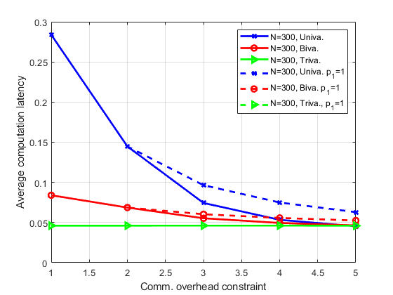
Figure 2: Average computation latency as a function of the communication overhead constraint for the different coding schemes.

VI Conclusion

We formulated the computation latency versus communication/complexity overheads trade off analysis in distributed coded computing systems. The overheads are defined relative to the resources required by outsourcing the computation to a single server in an uncoded manner. We presented two novel multivariate polynomial coding schemes supporting arbitrary matrix partitions, which, compared to univariate polynomial codes, require lower upload communication overheads at the cost of increasing the computation complexity. Simulation results show significant improvements in the computation latency for communication overhead constrained systems.

References

- [1] J. Dean and L. A. Barroso, “The tail at scale,” Communications of the ACM, vol. 56, pp. 74–80, 2013. [Online]. Available: http://cacm.acm.org/magazines/2013/2/160173-the-tail-at-scale/fulltext
- [2] K. Lee, M. Lam, R. Pedarsani, D. Papailiopoulos, and K. Ramchandran, “Speeding up distributed machine learning using codes,” IEEE Transactions on Information Theory, vol. 64, no. 3, pp. 1514–1529, 2017.
- [3] K. Lee, C. Suh, and K. Ramchandran, “High-dimensional coded matrix multiplication,” in 2017 IEEE International Symposium on Information Theory (ISIT). IEEE, 2017, pp. 2418–2422.
- [4] Q. Yu, M. A. Maddah-Ali, and A. S. Avestimehr, “Polynomial codes: An optimal design for high-dimensional coded matrix multiplication,” in Proc. Int’l Conf. on Neural Information Processing Systems, 2017, pp. 4406–4416.
- [5] ——, “Straggler mitigation in distributed matrix multiplication: Fundamental limits and optimal coding,” IEEE Transactions on Information Theory, vol. 66, no. 3, pp. 1920–1933, 2020.
- [6] S. Dutta, M. Fahim, F. Haddadpour, H. Jeong, V. Cadambe, and P. Grover, “On the optimal recovery threshold of coded matrix multiplication,” IEEE Transactions on Information Theory, vol. 66, no. 1, pp. 278–301, 2019.
- [7] W.-T. Chang and R. Tandon, “On the capacity of secure distributed matrix multiplication,” in 2018 IEEE Global Communications Conference (GLOBECOM), 2018, pp. 1–6.
- [8] R. G. L. D’Oliveira, S. El Rouayheb, and D. Karpuk, “Gasp codes for secure distributed matrix multiplication,” IEEE Transactions on Information Theory, vol. 66, no. 7, pp. 4038–4050, 2020.
- [9] X. Fan, A. Saldivia, P. Soto, and J. Li, “Coded matrix chain multiplication,” in 2021 IEEE/ACM 29th International Symposium on Quality of Service (IWQOS), 2021, pp. 1–6.
- [10] M. M. Amiri and D. Gündüz, “Computation scheduling for distributed machine learning with straggling workers,” IEEE Transactions on Signal Processing, vol. 67, no. 24, pp. 6270–6284, 2019.
- [11] L. Song, L. Tang, and Y. Wu, “An optimal coded matrix multiplication scheme for leveraging partial stragglers,” in 2023 IEEE International Symposium on Information Theory (ISIT). IEEE, 2023, pp. 1741–1744.
- [12] S. Kiani, N. Ferdinand, and S. C. Draper, “Exploitation of stragglers in coded computation,” in 2018 IEEE International Symposium on Information Theory (ISIT). IEEE, 2018, pp. 1988–1992.
- [13] E. Ozfatura, S. Ulukus, and D. Gündüz, “Straggler-aware distributed learning: Communication–computation latency trade-off,” Entropy, vol. 22, no. 5, p. 544, 2020.
- [14] A. Reisizadeh, S. Prakash, R. Pedarsani, and A. S. Avestimehr, “Coded computation over heterogeneous clusters,” IEEE Transactions on Information Theory, vol. 65, no. 7, pp. 4227–4242, 2019.
- [15] B. Hasırcıoǧlu, J. Gómez-Vilardebó, and D. Gündüz, “Bivariate polynomial codes for secure distributed matrix multiplication,” IEEE Journal on Selected Areas in Communications, vol. 40, no. 3, pp. 955–967, 2022.
- [16] B. Hasırcıoğlu, J. Gómez-Vilardebó, and D. Gündüz, “Bivariate polynomial coding for efficient distributed matrix multiplication,” IEEE Journal on Selected Areas in Information Theory, vol. 2, no. 3, pp. 814–829, 2021.
- [17] S. Dutta, Z. Bai, H. Jeong, T. M. Low, and P. Grover, “A unified coded deep neural network training strategy based on generalized polydot codes for matrix multiplication,” arXiv preprint arXiv:1811.10751, 2019.
- [18] R. A. Lorentz, Multivariate Birkhoff Interpolation. Springer, 2006.
- [19] G. Liang and U. C. Kozat, “Tofec: Achieving optimal throughput-delay trade-off of cloud storage using erasure codes,” in IEEE INFOCOM 2014-IEEE Conference on Computer Communications. IEEE, 2014, pp. 826–834.