Height-offset variables and pinning at infinity for gradient Gibbs measures on trees

Abstract.

We provide a general theory of height-offset variables and their properties for nearest-neighbor integer-valued gradient models on trees. This notion goes back to Sheffield [25], who realized that such tail-measurable variables can be used to associate to gradient Gibbs measures also proper Gibbs measures, via the procedure of pinning at infinity.

On the constructive side, our theory incorporates the existence of height-offset variables, regularity properties of their Lebesgue densities and concentration properties of the associated Gibbs measure. On the pathological side, we show that pinning at infinity necessarily comes at a cost. This phenomenon will be analyzed on the levels of translation invariance, the tree-indexed Markov chain property, and extremality.

The scope of our theory incorporates free measures, and also height-periodic measures of period $2$, assuming only finite second moments of the transfer operator which encodes the nearest neighbor interaction. Our proofs are based on investigations of the respective martingale limits, past and future tail-decompositions, and infinite product representations for moment generating functions.

Mathematics Subject Classifications (2020). 60K35 (primary); 82B41, 82B26 (secondary)

Key words. Localization, delocalization, gradient model, height-offset variable, pinning, martingale

1. Introduction

The notion of a gradient Gibbs measure (GGM) was introduced by Funaki and Spohn in [12] for the Ginzburg-Landau interface model to classify the ergodic measures for the shape of an interface in space which is subject to a stochastic dynamics. As opposed to Gibbs measures (GM), which describe the absolute heights of the interface, gradient Gibbs measures describe the heights of the interface modulo a joint shift in the height-direction. This can be represented by the field of increments (gradients) along the oriented edges of the respective graph.

For background on gradient models, on various graphs, concerning various aspects of localization and delocalization properties, see [4, 5, 6, 10, 26, 7, 19, 20, 22, 23, 24, 8, 5, 9]. In particular, [6, 10, 7, 8, 12, 25, 20] specifically consider gradient models on the lattice $\mathbb{Z}^{d}$ or the lattice torus $(\mathbb{Z}/nZ)^{d}$. On the other hand, [19] considers planar graphs of maximal degree three which are invariant under the action of some distinguished lattice $\mathcal{L}$ and provides two distinct sufficient assumptions on the interaction that guarantee that there are no (spatially) $\mathcal{L}$-invariant proper Gibbs measures. [24] studies the Ginzburg-Landau-model on locally finite connected graphs which are percolation-invariant in that for some $p<1$ the $p$-Bernoulli bond percolation on the respective graph almost surely possesses a transient infinite cluster. Finally, for results on the tree see [21, 4].

On the lattice $\mathbb{Z}^{d}$ the theory was significantly enhanced by Sheffield [25]. Amongst other results, for continuous spin variables Sheffield uniquely characterizes liftable extremal (or as he calls them smooth) gradient phases by their average heights modulo 1 and their height-offset spectrum. Here, an infinite-volume gradient state is liftable, if it arises as the projection of a proper Gibbs measure to the gradient variables. The height-offset spectrum is defined as the distribution of the underlying height-offset variable (HOV). Most importantly, a height-offset variable is by definition a tail-measurable observable on the infinite-volume state space of total height configurations $\Omega_{0}^{V}$ which enjoys covariance under a joint shift of the configuration in the height-direction. Height-offset variables make rigorous the idea of pinning a configuration at infinity, and can be used to lift gradient Gibbs measures to proper Gibbs measures, which describe absolute heights at the vertices of the graph. Remarkably, it turns out that this can be also possible in apparent delocalization regimes, if the respective gradient Gibbs measure is not extreme in the set of all gradient Gibbs measures. This may seem to be a contradiction at first, and there is in fact an interesting general theory behind, as we will see. To our knowledge the phenomenon was first shown to appear with a concrete example of a model on a tree, in the inspiring paper [21], where Lammers and Toninelli discuss how to interpret the free state of the graph homomorphism model (cf. also e.g., [3] for the same model on the lattice) on regular trees as a proper Gibbs measure, using the existence of a non-trivial height-offset variable. Their model is nice but also very particular. So it remained unclear, how far the phenomenon extends when one looks at general gradient interactions. Are there always HOVs, and if so, what regularity properties do they have? What are the possible consequences, are there pinned measures, what is their structure? What can we say about extremality, Markov chain property, translation invariance? This begs for a general theory for HOVs for general gradient Gibbs measures on trees. This is the motivation for our present work.

The most prominent and popular type of GGMs for which our theory holds, are free states, obtained with open boundary conditions. Moreover, we can include in our analysis, at not too much more cost, also the case of the more complex period-$2$ height-periodic GGMs. Let us give an idea of how these interesting measures can be constructed. For general integer-valued gradient models on regular trees, described via a transfer operator $Q$, [16, 14, 15, 1], provided period-$q$ height-periodic GGMs via a two layer hidden Markov model construction with an internal layer $\mathbb{Z}_{q}$. The hidden variables on the internal layer interact via a suitably chosen $q$-dependent Hamiltonian. The full measure on integer-valued increments is obtained from here via application of transition kernels acting on the edges. The classes of these GGMs associated with different coprime values of $q$ were then shown to be disjoint. Furthermore, for any summable isotropic $Q$ there always exist non-translation invariant gradient Gibbs measures corresponding to an internal layer with sufficiently large (depending on $Q$) $q$ (see [15]). On the more concrete side, such height-periodic GGMs naturally show up via non-normalizable periodic boundary law solutions to the $Q$-dependent tree recursions [16]. This is related to but goes beyond Zachary [27] as he studies normalizable boundary law solutions.

Main results 1: Existence of HOVs and peculiarities of pinned measures

In the present note we consider free states and height-periodic measures asking for the possibility of pinning at infinity. Specifically we will explain how to obtain in complete generality the existence of height-offset variables for free GGMs and GGMs of period $2$. To show existence of HOVs, we prove that limits of empirical height sums over spheres (after an arbitrary pinning) converge a.s. and in $L^{2}(\nu)$ to a height-offset variable $H$. This works for the free gradient measure $\nu$, see Proposition 1, but also for height-period $2$ gradient measures, see Proposition 2 under an $L^{2}$-condition on the defining a-priori increment interaction along any edge described by $Q$.

For convenience of the reader, and to be on safe grounds to develop the theory, we include a detailed proof of how to pin at infinity on trees by means of an HOV and obtain a GM from the GGM. From here we derive consequences in our paper, both from a structural probabilistic point of view, and from a quantitative analytical point of view. Namely, this pinned-at-infinity measure however, always has peculiar properties: It necessarily loses translation invariance (tree-automorphism invariance resp.). See Proposition 5. Moreover, it loses extremality and in case of the free state even more the tree-indexed Markov chain property, see Proposition 7.

Main results 2: Regularity properties of HOVs

Having proved existence of HOVs we turn to describe their distribution, and also to derive consequences for the marginal distribution of the height-variable of the pinned GGM at the origin of the tree.

The distribution of the HOV can be analyzed nicely for the free measure on the level of the characteristic function (and the moment generating function whenever it exists). To to so, we exploit the recursive structure of the tree, from which we are able to derive Propositions 3 and 4 in terms of an infinite product of the corresponding quantities of $Q/\|Q\|_{1}$, see Lemma 1.

Without any further assumption on $Q$ beyond existence of second moments, we obtain exponential upper bounds on the Fourier-transform, which imply existence of an infinitely often differentiable Lebesgue-density of the HOV, see Proposition 4.

Assuming moreover that the moment generating function of the increment along any oriented edge has a positive radius of convergence $R>0$, we can deduce the existence of the moment generating for the HOV, too, with enlarged radius of convergence $R(d+1)$. Moreover, we obtain a nice relation between the cumulants.

For period-2 GGMs the situation is a little more intricate, but we are able to obtain bounds instead of equalities: For the characteristic function of the HOV again exponential upper bounds can be derived, which implies that the density is infinitely-often differentiable. The nice explicit relations for the cumulants we obtained for the free measure are not valid anymore, but still we get bounds which can be used to obtain tail-estimates.

To round up our analysis, we present the two cases of the SOS-model and for the discrete Gaussian (cf. also e.g., [2] for recent results on the lattice).

The remainder of the paper is organized as follows: Following a short overview of the definitions and notions in Subsection 2.1 we present all results regarding pinning at infinity of the free state summarized in Theorem 2. The corresponding results regarding gradient Gibbs measures of height-period $2$ are then given in analogous Theorem 3. In Section 3 we provide the proofs of each of the statements of Theorems 2 and 3 in the same order as they appear in the respective theorem and structured by subsections whose titles summarize the key idea of proof. Each of these subsections begins with a proof of the respective statement for the easier case of the free state and ends with an extension to the more intricate case of gradient Gibbs measures of height-period $2$.

2. Definitions and main results

2.1. Preliminary definitions

In the following, we let $\mathbb{T}^{d}=(V,E)$ denote the Cayley tree of order $d$, i.e., every vertex has exactly $d+1$ nearest neighbors with vertex set $V$, (unoriented) edge set $E$ and root $\rho$. Besides $E$, we also consider the set $\vec{E}$ consisting of oriented pairs of vertices connected by an edge. We will partition $\vec{E}={}^{\rho}\vec{E}\cup\vec{E}^{\rho}$, where ${}^{\rho}\vec{E}$ denotes those oriented edges which point away from the root $\rho$ and $\vec{E}^{\rho}$ is the complementary subset of those edges which point towards $\rho$.

We will write $\Lambda\Subset V$ if $\Lambda$ is a finite subset and denote by $\partial\Lambda\subset V$ its outer boundary. For any $x,y\in V$ we will further denote by $\Gamma(x,y)$ the unique directed path from $x$ to $y$.

Furthermore, for any $r\in\mathbb{N}$ we denote by $W_{r}:=\{v\in V\colon d(\rho,v)=r\}$ the sphere of radius $r$ and by $B_{r}:=\{v\in V\colon d(\rho,v)\leq r\}$ the closed ball of radius $r$. Finally, for any $u\in V$ we denote by $S(u):=\{v\in V\colon\{u,v\}\in E\text{ and }d(v,\rho)=d(u,\rho)+1\}$ the set of children (direct successors) of $v$. Within some of the proofs given in Section 3 we will also consider the $d$-ary tree, where the root has degree $d$ and every other vertex has degree $d+1$, which means that each vertex has exactly $d$ children.

Height-configurations and gradient configuration

Let $\Omega:=\mathbb{Z}^{V}=\{(\omega_{x})_{x\in V}\mid\omega_{x}\in\mathbb{Z}\}$ denote the set of (integer-valued) height-configurations endowed with the product-$\sigma$-algebra $\mathcal{F}=\mathcal{P}(\mathbb{Z})^{\otimes V}$ generated by the spin-variables (projections) $\sigma_{y}:\Omega\rightarrow\mathbb{Z},\ \omega\mapsto\omega_{y}$, where $y\in V$. For arbitrary $\Lambda\subset V$ we denote by $\mathcal{F}_{\Lambda}$ the $\sigma$-algebra on $\Omega$ generated by the spin-variables for vertices inside $\Lambda$.

Besides the height-configurations $\Omega$, we consider the set of gradient configurations $\Omega^{\nabla}:=\{(\zeta_{(u,v)})_{(u,v)\in\vec{E}}\in\mathbb{Z}^{\vec{E}}\mid\zeta_{(u,v)}=-\zeta_{(v,u)}\}$, which describe height-increments along directed edges instead of absolute heights. The corresponding gradient-projection reads $\nabla:\Omega\rightarrow\Omega^{\nabla};\ (\omega_{x})_{x\in V}\mapsto(\omega_{x}-\omega_{y})_{(x,y)\in\vec{E}}$ with gradient spin-variables $\eta_{(x,y)}(\zeta):=\zeta_{(x,y)}$, which generate the respective gradient sigma-algebra $\mathcal{F}^{\nabla}:=\mathcal{P}(\mathbb{Z})^{\otimes\vec{E}}$ on $\Omega^{\nabla}$. Given any gradient configuration $\zeta\in\Omega^{\nabla}$, let $\sigma^{x,s}(\zeta)\in\Omega$ denote the height configuration obtained from $\zeta$ by pinning the height to be $s$ at vertex $x$. In particular, $\Omega^{\nabla}$ is one-to-one to the set $\Omega/\mathbb{Z}$ of height-configurations modulo joint height-shifts of the form $\tau_{a}:\Omega\rightarrow\Omega;\ (\omega_{x})_{x\in V}\mapsto(\omega_{x}-a)_{x\in V}$ for some $a\in\mathbb{Z}$.

Transfer operators and Markovian Gibbsian specifications.

By a transfer operator on $\mathbb{T}^{d}$ we mean a function $Q:\mathbb{Z}\rightarrow(0,\infty)$ which is symmetric (i.e., $Q(-i)=Q(i)$ for every $i\in\mathbb{Z}$) and satisfies $Q\in\ell^{\frac{d+1}{2}}(\mathbb{Z})$ in that $\|Q\|_{\frac{d+1}{2}}:=\left(\sum_{i\in\mathbb{Z}}Q(i)^{\frac{d+1}{2}}\right)^{\frac{2}{d+1}}<\infty$. The idea behind is that the transfer operator is usually given in terms of a suitable symmetric interaction function $U:\mathbb{Z}\rightarrow[0,+\infty)$ as

$$Q(i)=e^{-\beta U(i)},$$ (2.1)

where $\beta>0$ is interpreted as the inverse of a temperature.

A transfer operator $Q$ induces the (local) Markovian Gibbsian specification

$$\gamma=\{\gamma_{\Lambda}:\mathcal{F}\times\Omega\rightarrow[0,1]\}_{\Lambda\Subset V}$$

by the assignment

$$\gamma_{\Lambda}(\sigma_{\Lambda}=\tilde{\omega}_{\Lambda}\mid\omega)=\frac{1}{Z_{\Lambda}(\omega_{\partial\Lambda})}\left(\prod_{\{x,y\}\in E_{\Lambda}}Q(\tilde{\omega}_{x}-\tilde{\omega}_{y})\right)\,\prod_{\genfrac{}{}{0.0pt}{}{\{x,y\}\in E}{x\in\Lambda,y\in\partial\Lambda}}Q(\tilde{\omega}_{x}-\omega_{y}),$$ (2.2)

for every $\Lambda\Subset V$, $\tilde{\omega}\in\Omega_{\Lambda}$ and $\omega\in\Omega$. Here, the partition function $Z_{\Lambda}$ gives for every $\omega\in\Omega$ the normalization constant $Z_{\Lambda}(\omega)=Z_{\Lambda}(\omega_{\partial\Lambda})$ turning $\gamma_{\Lambda}(\cdot\mid\omega)$ into a probability measure on $(\Omega,\mathcal{F})$ and $\omega_{\Lambda}$, $\Omega_{\Lambda}$, $E_{\Lambda}$ and $\vec{E}_{\Lambda}$ denote the respective restrictions on $\Lambda\subset V$, where edges in $E_{\Lambda}$ or $\vec{E}_{\Lambda}$ are supposed to have both vertices inside $\Lambda$. The assumptions $Q>0$ and $Q\in\ell^{\frac{d+1}{2}}(\mathbb{Z})$ guarantee that such a partition function does exist. See Lemma 1 in [14].

The kernels $\gamma_{\Lambda}$ can be projected to the respective gradient Gibbs specification

$$\gamma^{\nabla}=\{\gamma^{\nabla}_{\Lambda}:\mathcal{F}^{\nabla}\times\Omega^{\nabla}\rightarrow[0,1]\}_{\Lambda\Subset V}.$$

For this we note that for any $\emptyset\neq\Lambda\Subset V$ the gradient variables in the disconnected complement $\Lambda^{c}$ do not contain information on the relative heights at the boundary $[\omega]_{\partial\Lambda}\in\mathbb{Z}^{\partial\Lambda}\mod\mathbb{Z}$, where $[\tilde{\omega}]_{\partial\Lambda}=[\omega]_{\partial\Lambda}$ if and only if $\tilde{\omega}_{\partial\Lambda}=\left(\tau_{a}(\omega)\right)_{\partial\Lambda}$ for some $a\in\mathbb{Z}$. However, in any case the map $\Omega\ni\omega\mapsto[\omega]_{\partial\Lambda}\in\mathbb{Z}^{\partial\Lambda}\mod\mathbb{Z}$ is clearly measurable with respect to the whole gradient field $\mathcal{F}^{\nabla}$ as any $x,y\in\partial\Lambda$ are connected by a path in $V$. Hence, the kernels $\gamma^{\nabla}_{\Lambda}$ are

$$\gamma^{\nabla}_{\Lambda}(\eta_{\Lambda}=\zeta_{\Lambda}\mid\zeta):=\gamma_{\Lambda}(\sigma_{\Lambda}=\omega_{\Lambda}\mid\omega)$$ (2.3)

for any $\omega\in\Omega$ such that $(\nabla\omega)_{\Lambda^{c}}=\zeta_{\Lambda^{c}}$ and $[\nabla\omega]_{\partial\Lambda}=[\zeta]_{\partial\Lambda}$. In what follows we call the respective $\sigma$-algebra

$$\mathcal{T}_{\Lambda}^{\nabla}:=\sigma\left((\eta_{(x,y)})_{(x,y)\in\vec{E}_{\Lambda^{c}}},\ [\cdot]_{\partial\Lambda}\right)$$

on $\Omega^{\nabla}$ the outer gradient $\sigma$-algebra for $\Lambda$.

Gibbs measures and gradient Gibbs measures.

A probability measure $\mu$ on $(\Omega,\mathcal{F})$ is called a Gibbs measure for the specification $\gamma$ iff the DLR-equation holds

$$\int_{\Omega}\gamma_{\Lambda}(A\mid\omega)\mu(d\omega)=\mu(A)\quad\text{ for every }A\in\mathcal{F}\text{ and }\Lambda\Subset V.$$ (2.4)

Similarly, a gradient measure $\nu$ on $(\Omega^{\nabla},\mathcal{F}^{\nabla})$ is called a gradient Gibbs measure for the gradient specification $\gamma^{\nabla}$ iff the DLR-equation holds

$$\int_{\Omega^{\nabla}}\gamma_{\Lambda}^{\nabla}(A\mid\zeta)\mu(d\zeta)=\mu(A)\quad\text{ for every }A\in\mathcal{F}^{\nabla}\text{ and }\Lambda\Subset V.$$ (2.5)

Tree-indexed Markov chains.

Following [13, Chapter 12], choosing any oriented edge $(u,v)\in\vec{E}$ of the tree induces a splitting of the sets of vertices $V$ into the past

$$[-\infty,uv):=\{w\in V\mid\text{d}(w,u)<\text{d}(w,v)\}$$ (2.6)

and the future $[uv,+\infty):=V\setminus[-\infty,uv)$. See also Figure 2 below for an illustration. Then, a probability measure $\mu$ on $(\Omega,\mathcal{F})$ is by definition a tree-indexed Markov chain iff for every $(u,v)\in\vec{E}$

$$\mu(\sigma_{v}=\cdot\mid\mathcal{F}_{[\infty,uv)})=\mu(\sigma_{v}=\cdot\mid\mathcal{F}_{\{u\}})\quad\mu-\text{a.s.}$$ (2.7)

Liftable gradient Gibbs measures

While every Gibbs measure can be projected to a gradient Gibbs measure for the respect gradient specification via the map $\nabla$, which sends a spin configuration to its gradients, the converse is not generally true. This distinction corresponds to whether a gradient Gibbs measure is liftable (or smooth in the sense of Sheffield[25]) in that it can be lifted to a proper Gibbs measure, or not.

Definition 1.

A function $H:\Omega\rightarrow\mathbb{R}\cup\{\pm\infty\}$ is called a height-offset variable for a gradient Gibbs measure $\nu$ iff it fulfills the following properties:

1. For all $a\in\mathbb{Z}$ we have $H(\omega+a)=H(\omega)+a$ for all $\omega\in\Omega$;

2. $H$ is measurable with respect to the tail-$\sigma$-algebra $\mathcal{T}$ on $\Omega$;

3. $\nu(|H|<\infty)=1$.

For c) note that by a) the event $\{|H|<\infty\}$ is measurable with respect to $\mathcal{F}^{\nabla}$.

For a height-offset variable $H$ let $\Omega^{\nabla}_{H}:=\Omega^{\nabla}\cap\{|H|<\infty\}$. Then, for fixed $x\in V$ and $s\in\mathbb{Z}$ define the map

$$G_{H}:\Omega_{H}^{\nabla}\rightarrow\Omega;\ G_{H}(\zeta):=\sigma^{x,s}(\zeta)-\lfloor H(\sigma^{x,s}(\zeta))\rfloor,$$ (2.8)

where $\lfloor\alpha\rfloor$ denotes the largest integer less or equal to $\alpha\in\mathbb{R}$. Note that by definition of a height-offset variable the definition of the function $G_{H}$ is independent of the choices of $x$ and $s$, as $\sigma^{y,t}(\zeta)=\sigma^{x,s}(\zeta)+(t-s)-\sum_{b\in\Gamma(x,y)}\zeta_{b}$. In particular, this implies that the image measure $\mu^{H}:=\nu\circ G_{H}^{-1}\in\mathcal{M}_{1}(\Omega,\mathcal{F})$ has single-site marginals given by

$$\mu^{H}(\sigma_{x}=t)=\nu(\,\lfloor H(\sigma^{x,0})\rfloor=-t)=\nu(\sum_{b\in\Gamma(\rho,x)}\eta_{b}-\,\lfloor H(\sigma^{\rho,0})\rfloor=t),\quad t\in\mathbb{Z}$$ (2.9)

So, we see that the Gibbs measure is obtained from the gradient Gibbs measure with fluctuating localization center $\lfloor H\rfloor$.

Theorem 1 (Gibbs property of measures pinned at infinity).

Let $\nu$ be a gradient Gibbs measure for $\gamma^{\nabla}$ which possesses a height-offset variable $H$.

Then the image measure $\mu^{H}=\nu\circ G_{H}^{-1}\in\mathcal{M}_{1}(\Omega,\mathcal{F})$ is a Gibbs measure for $\gamma$.

The Theorem goes back to Sheffield [25] and Lammers and Toninelli [21], but for convenience of the reader we include a detailed proof in the Appendix.

Remark 1.

Theorem 1 above does not impose any assumptions on regularity of the tree $(V,E)$ or on symmetries of the gradient Gibbs measure $\nu$.

We will construct height-offset variables as the limit of spherical averages of height configurations. To verify that this limit exists as a real-valued random variable on $\Omega$ $\nu$-almost surely, we will also consider spherical averages of gradient fields with a prescribed absolute height at the root.

Definition 2 (Spherical averages of height- and pinned gradient configurations).

1. We denote by $H_{r}:\Omega\rightarrow\mathbb{R}$

   $$H_{r}(\omega):=\frac{1}{|W_{r}|}\sum_{v\in W_{r}}\omega_{v}$$ (2.10)

   the average value of the heights at the $r$-sphere, $r\in\mathbb{N}$.

2. Furthermore, by $H^{\nabla}_{r}:\Omega^{\nabla}\rightarrow\mathbb{R}$

   $$H^{\rho,0}_{r}(\zeta):=\frac{1}{|W_{r}|}\sum_{v\in W_{r}}\sigma_{v}^{\rho,0}(\zeta)$$ (2.11)

   we denote the average value of the heights of the gradient field pinned at height zero at the root $\rho$, $r\in\mathbb{N}$.

Remark 2.

We have $H_{r}(\omega)=H_{r}^{\rho,0}(\nabla\omega)+\omega_{\rho}$ for every $r\in\mathbb{N}$ and $\omega\in\Omega$.

Assumption 1 (Second moment condition on transfer operator $Q$).

In the following Theorems 2 and 3 we assume that

$$\sum_{j\in\mathbb{Z}}j^{2}Q(j)<\infty,$$ (2.12)

which means that the probability measure on $\mathbb{Z}$ described by the probability mass function $\frac{Q(\cdot)}{\|Q\|_{1}}$ has finite second moments.

2.2. Result: Pinning at infinity for free state under second moment assumption on transfer operator

At first, we show that the gradient Gibbs measure which arises for free boundary conditions can be pinned at infinity.

Definition 3 (Free state of i.i.d-increments).

Given a positive symmetric transfer operator $Q\in\ell^{\frac{d+1}{2}}(\mathbb{Z})$, we call the probability measure $\nu$ on $(\Omega^{\nabla},\mathcal{F}^{\nabla})$ with marginals

$$\nu(\eta_{\Lambda\cup\partial\Lambda}=\zeta_{\Lambda\cup\partial\Lambda})=\frac{1}{Z_{\Lambda}}\prod_{(x,y)\in{}^{\rho}\vec{E}_{\Lambda\cup\partial\Lambda}}Q(\zeta_{(x,y)}).$$ (2.13)

the free state (of i.i.d.-increments).

With that notation in mind, the result reads

Theorem 2 (Pinning at infinity of the free state: existence, regularity of density, loss of translation invariance and of Markov property).

Let $Q:\mathbb{Z}\rightarrow(0,\infty)$ be any positive symmetric transfer operator of gradient type such that $\sum_{j\in\mathbb{N}}j^{2}Q(j)<\infty$. Then the following holds true for the corresponding free state $\nu$ on the Cayley tree of order $d\geq 2$.

• Let $(H_{r})_{r\in\mathbb{N}}$ be as in Definition 2. Then $H:=\lim_{r\rightarrow\infty}H_{r}$ is a height-offset variable for $\nu$ in the sense of Definition 1, where the limit holds $\nu$-almost surely and in $\mathcal{L}^{2}(\nu)$. In particular, the measure $\mu^{H}$ associated with $H$ and $\nu$ via Theorem 1 is a proper Gibbs measure.

• The corresponding distribution of $H^{\rho,0}$ obtained from Definition 2 under $\nu$ has an infinitely often differentiable Lebesgue-density $f_{H^{\rho,0}}$. Moreover, for every $\delta>0$ there exist some lattice $\mathfrak{R}_{\delta}\subset\mathbb{R}$ of the form $\mathfrak{R}_{\delta}=a+\delta\mathbb{Z}$, where $a\in\mathbb{R}$, such that $f_{H^{\rho,0}}$ is strictly positive on $\mathfrak{R}_{\delta}$.

• Assume that there is some $R>0$ such that the moment generating function for a single gradient variable, $t\mapsto\sum_{j\in\mathbb{Z}}\exp(tj)\frac{Q(j)}{\|Q\|_{1}}$ is finite for $t\in(-R,+R)$. Then, for every $A<(d+1)R$ there exists a $B(A)\in(0,\infty)$ such that the single-site marginal at the root satisfies the following exponential concentration:

  $$\mu^{H}(|\sigma_{\rho}|\geq s)\leq B(A)\exp(-As),\quad\text{for every }s\in\mathbb{N}.$$

• The lifted measure Gibbs $\mu^{H}$ is necessarily not invariant under the translations of the tree.

• The measure $\mu^{H}$ is not a tree-indexed Markov chain and in particular not extreme in the set of all Gibbs measures for the specification associated with $Q$ via (2.2).

2.3. Result: Pinning at infinity for the hidden Ising model under second moment assumption on transfer operator

Spatially homogeneous gradient Gibbs measures for underlying hidden clock models were introduced in [16, 18] in the context of a height-periodicity approach towards Zachary’s [27] boundary law-equation for those Gibbs measures on the tree which are also tree-indexed Markov chains. The notion was refined and extended in [15] to provide a broad statement on existence of gradient Gibbs measures which are not invariant under the automorphisms of the tree, requiring only a summability assumption on the transfer operator $Q$. We shortly present the construction for the special case of a hidden Ising model and afterwards state Theorem 3, which analogously to Theorem 2 above for the free state describes the existence and properties of a suitable HOV for this class of GGM.

Let $\mathbb{Z}_{2}=\mathbb{Z}/2\mathbb{Z}=\{\bar{0},\bar{1}\}$. For any positive symmetric $Q\in\ell^{1}(\mathbb{Z})$ define the fuzzy transfer operator $\bar{Q}:\mathbb{Z}_{2}\rightarrow(0,\infty)$ by setting

$$\bar{Q}(\bar{0}):=\sum_{l\in\mathbb{Z}}Q(2l)\text{ and }\bar{Q}(\bar{1}):=\sum_{l\in\mathbb{Z}}Q(1+2l).$$ (2.14)

The fuzzy transfer operator $\bar{Q}$ describes an Ising model in the following sense: if we identify $\bar{0}$ with $-1$ and $\bar{1}$ with $+1$ then $\bar{Q}$ then the formal Ising-Hamiltonian

$$\mathcal{H}(\tilde{\omega})=-J\sum_{x\sim y}\tilde{\omega}_{x}\tilde{\omega}_{y},\quad\tilde{\omega}\in\{\pm 1\}^{V}$$

is built from $\bar{Q}$ via

$$\exp(2J)=\frac{\bar{Q}(\bar{0})}{\bar{Q}(\bar{1})}.$$

In the following we will write $\bar{a}:=a+2\mathbb{Z}$ to denote the projection of $a\in\mathbb{Z}$ to $\mathbb{Z}_{2}$. Fix any Gibbs measure $\bar{\mu}$ on $\mathbb{Z}_{2}^{V}$ with spin-variables $(\bar{\sigma}_{v})_{v\in V}$ for the Ising model described by $\bar{Q}$. Then we consider the following two-step procedure, where we first sample a configuration of $\mathbb{Z}_{2}$-valued spins (fuzzy chain) which plays the role of a random environment. Given a realization of such an environment we then sample edge-wise independently integer-valued increments conditionally on whether the fuzzy chain changes or preserves its value along the respective edge according to the kernel

$$\rho^{Q}(s\mid\bar{a}):=\boldsymbol{1}_{a+2\mathbb{Z}}(s)\frac{Q(s)}{\bar{Q}(\bar{a})},\quad s\in\mathbb{Z},\ \bar{a}\in\{\bar{0},\bar{1}\}.$$ (2.15)

Definition 4.

Let $\bar{\mu}$ be a Gibbs measure for the Ising model defined by $\bar{Q}$. Then we call the annealed measure $\nu^{\bar{\mu}}$ on $(\Omega^{\nabla},\mathcal{F}^{\nabla})$ with marginals

$$\begin{split}\nu^{\bar{\mu}}(\eta_{\Lambda\cup\partial\Lambda}=\zeta_{\Lambda\cup\partial\Lambda})=\frac{1}{Z_{\Lambda\cup\partial\Lambda}}\sum_{\bar{\omega}_{\Lambda\cup\partial\Lambda}\in\mathbb{Z}_{2}^{\Lambda\cup\partial\Lambda}}\bar{\mu}(\bar{\sigma}_{\Lambda\cup\partial\Lambda}=\bar{\omega}_{\Lambda\cup\partial\Lambda})\prod_{(x,y)\in{}^{\rho}\vec{E}_{\Lambda\cup\partial\Lambda}}\rho^{Q}(\zeta_{(x,y)}\mid\bar{\omega}_{y}-\bar{\omega}_{x}),\end{split}$$ (2.16)

where $\Lambda\Subset V$, the gradient Gibbs measure of height period $2$ associated with the hidden Ising measure (or fuzzy chain) $\bar{\mu}$.

In cases where we do not want to make fuzzy chain $\bar{\mu}$ explicit we will write $\nu^{per}$ instead.

The gradient measure $\nu^{\bar{\mu}}$ indeed satisfies the DLR-equation, for a proof see [15, Theorem 2], where we note that the construction does not impose any further assumption such as spatial homogeneity on the hidden Ising measure $\bar{\mu}$ and, even more, generalizes from the hidden Ising model to more general hidden clock models on $\mathbb{Z}_{q}$, $q\geq 2$.

For the Statement (b2) of the following result on pinning at infinity the GGM for the hidden Ising model we need to consider the moment generating function of the $\mathbb{Z}$-valued increment along an edge conditioned on the increment of the internal fuzzy chain along the edge.

Definition 5 (Upper bound on single-edge moment generating function in hidden Ising model).

Consider the hidden Ising model with fuzzy chain $(\bar{\sigma}_{u})_{u\in V}$ and let $(u,v)\in\vec{E}$ be any edge. Then we define

$$\hat{\psi}^{per}_{\star}(t):=\max_{\bar{a}\in\{\bar{0},\bar{1}\}}\big{|}\,\mathbb{E}[\exp(t\eta_{(v,w)})\mid\bar{\sigma}_{w}-\bar{\sigma}_{v}=\bar{a}]\,\big{|},\quad t\in D_{\hat{\psi}^{per}},$$ (2.17)

where $D_{\hat{\psi}^{per}}\subset\mathbb{C}$ denotes the respective domain of convergence, where the expression exists as a finite number. Note that by symmetry of the conditional distribution (cf. Equation (3.11) below) the expression $\hat{\psi}^{per}_{\star}(is)$ is well-defined and real for all $s\in\mathbb{R}$ and provides a corresponding upper bound for the absolute value of the characteristic function.

Now the theorem reads:

Theorem 3 (Pinning at infinity for gradient Gibbs measures of height period $2$: existence, regularity of density, loss of translation invariance and loss of extremality).

Let $Q:\mathbb{Z}\rightarrow(0,\infty)$ be a positive symmetric transfer operator of gradient type such that $\sum_{j\in\mathbb{N}}j^{2}Q(j)<\infty$. Let $\bar{\mu}$ be any (not necessarily spatially homogeneous) tree-indexed Markov chain Gibbs measure for the Ising model with interaction described by $\bar{Q}$ (see Eq. (2.14)). Then the following holds true for the gradient Gibbs measure $\nu^{\bar{\mu}}$ of height-period $2$ associated to $\bar{\mu}$ on the $d$-regular tree with $d\geq 2$ via Definition 4.

• Let $(H_{r})_{r\in\mathbb{N}}$ be as in Definition 2. Then $H:=\limsup_{r\rightarrow\infty}H_{r}\in\mathcal{L}^{2}(\nu^{\bar{\mu}})$ is a HOV for $\nu^{\bar{\mu}}$. In particular, the associated measure $\mu^{H}$ which is pinned at infinity via $\mu^{H}=\nu^{\bar{\mu}}\circ G_{H}^{-1}$ (cf. Eq. (2.8)) is a proper Gibbs measure.

• The corresponding distribution of $H^{\rho,0}$ obtained from Definition 2, under $\nu^{\bar{\mu}}$, has an infinitely often differentiable Lebesgue-density $f_{H^{\rho,0}}$. Moreover, for every $\delta>0$ there exist some lattice $\mathfrak{R}_{\delta}\subset\mathbb{R}$ of the form $\mathfrak{R}_{\delta}=a+\delta\mathbb{Z}$, where $a\in\mathbb{R}$, such that $f_{H^{\rho,0}}$ is strictly positive on $\mathfrak{R}_{\delta}$.

• Assume that there is some $R>0$ such that the single-edge function $\hat{\psi}^{per}_{\star}(t)$ given by Definition 5 is finite for $t\in(-R,+R)$. Then, for every $A<(d+1)R$ there exists a $B(A)\in(0,\infty)$ such that the single site marginal at the root satisfies the following exponential decay:

  $$\mu^{H}(|\sigma_{\rho}|\geq s)\leq B(A)\exp(-As),\quad\text{for every }s\in\mathbb{N}.$$

• The lifted Gibbs measure $\mu^{H}$ is necessarily not invariant under the translations of the tree.

• The $\mu^{H}$ is not extreme in the set of all Gibbs measures for $Q$.

Remark 3.

• Property (b1) in Theorems 2 and 3 implies that the support of the distribution of $H^{\rho,0}$ equals $\mathbb{R}$.

• In the case $q=2$ conditioning on the non-observable internal fuzzy spin preserves the $\pm$-symmetry (see (3.12) below, and thus leads to the martingale property of $(H_{r}^{\rho,0})_{r\in\mathbb{N}}$ even conditional on the internal spins, which will be very useful for the proofs given below. This is in general no longer true for higher $q$. Hence, the convergence of $H_{r}$, if it holds at all for general $q$, would need to be proved in a way different from conditioning on the internal spins.

3. Proofs

We will prove each of the Statements (a), (b1), (b2), (c1) and (c2) of the Theorems 2 and 3 in a separate subsection. We begin with the first part of Statement (a) on almost sure convergence of the family $(H_{r})_{r\in\mathbb{N}}$, which follows from identifying the process as a suitable $\mathcal{L}^{2}$-Martingale for a suitable filtration. Afterwards, we study the moment generating functions associated with $(H_{r})_{r\in\mathbb{N}}$ to obtain Statement (b2) on localization of the single-site marginals of the measure $\mu^{H}$. Subsequently, we give the proof of the first part of Statement (b1) on absolute continuity of the distribution of the HOV $H$, which follows from considering the characteristic functions associated with $(H_{r})_{r\in\mathbb{N}}$, and is thus merely a corollary of the previous calculations with moment generating functions (two-sided Laplace transforms). Before proving the second part of Statement (b1) regarding the support of the Lebesgue density, we first present the more illustrative proof of Statement (c1) on non-invariance of the pinned measure under the translations of the tree. This is based on splitting the tree into the two sub-trees of the past and of the future of an edge and analyzing a reflection that changes the roles of infinite past and future. This is followed by the proof of the second part of Statement (b1) which relies on another decomposition of the tree. Finally, we conclude with a proof of Statement (c2) on violation of the Markov property and non-extremality.

We present the respective steps for the free state and the GGM for the hidden Ising model as much in parallel as possible to avoid redundancies in argumentation and to keep presentation short and concise.

3.1. Averages over spheres form a suitable $\mathcal{L}^{2}$-martingale

To show that $\limsup_{r\rightarrow\infty}H_{r}$ is $\nu$-almost surely finite, in what follows, we consider the function $H_{r}^{\rho,0}$ (cf. Definition 2) which maps any gradient configuration $\zeta$ to the average height at the $r$-sphere, where we pin the height $0$ at the root $\rho$.

Proposition 1 (Martingale construction for the free state).

Let $Q$ be a positive symmetric transfer operator with $\sum_{j=0}^{\infty}j^{2}Q(j)<\infty$. Then for the free state $\nu^{free}$, the family $(H_{r}^{\rho,0})_{r\in\mathbb{N}}$ is an $\mathcal{L}^{2}(\nu^{free})$-martingale with respect to the filtration $(\mathcal{F}^{\nabla}_{B_{r}})_{r\in\mathbb{N}}$. Hence, $(H_{r}^{\rho,0})_{r\in\mathbb{N}}$ converges $\nu^{free}$-a.s. and in $\mathcal{L}^{2}(\nu^{free})$ to a limit $H^{\rho,0}$, which is $\nu^{free}$-a.s. finite.

Proof of Proposition 1.

The family $(H_{r}^{\rho,0})_{r\in\mathbb{N}}$ is by construction adapted to the filtration $\mathcal{F}^{\nabla}_{B_{r}}$. To prove the martingale property, let $r\in\mathbb{N}$. Then linearity of the conditional expectation and the Markov property give $\nu^{free}$-a.s.

$$\begin{split}\mathbb{E}[H^{\rho,0}_{r+1}\mid\mathcal{F}^{\nabla}_{B_{r}}]&=\frac{1}{|W_{r}|}\sum_{u\in W_{r}}\frac{1}{d}\sum_{v\in S(u)}\mathbb{E}[\sigma_{v}^{\rho,0}\mid\mathcal{F}^{\nabla}_{B_{r}}]=\frac{1}{|W_{r}|}\sum_{u\in W_{r}}\frac{1}{d}\sum_{v\in S(u)}\mathbb{E}[\sigma_{v}^{\rho,0}\mid\sigma_{u}]\end{split}$$ (3.1)

From the fact that $\nu(\sigma_{x}=i\mid\sigma_{y}=j)=\frac{Q(i-j)}{\|Q\|_{1}}$ and symmetry of $Q$ it follows that for every $u\in W_{r}$ and $v\in S(u)$

$$\mathbb{E}[\sigma_{v}^{\rho,0}\mid\sigma_{u}](\omega)=\omega_{u}\quad\nu^{free}{\text{-}a.s.}$$ (3.2)

Inserting this into (3.1) shows the martingale property.

In the second step, we show $\mathcal{L}^{2}(\nu)$-boundedness of the martingale $(H_{r}^{\rho,0})_{r\in\mathbb{N}}$ to deduce from martingale convergence [17, Corollary 11.11] that $(H_{r}^{\rho,0})_{r\in\mathbb{N}}$ converges $\nu^{free}$-a.s. to a real-valued limiting random variable.

We have

$$\begin{split}\mathbb{E}[(H_{r}^{\rho,0})^{2}]=\frac{1}{|W_{r}|^{2}}\sum_{u,v\in W_{r}}\mathbb{E}[\sigma_{u}^{\rho,0}\sigma_{v}^{\rho,0}]&=\frac{1}{|W_{r}|}\sum_{v_{2}\in W_{r}}\mathbb{E}[\sigma_{v_{1}}^{\rho,0}\sigma_{v_{2}}^{\rho,0}],\end{split}$$ (3.3)

where $v_{1}\in W_{r}$ is any fixed vertex. For any $v_{2}\in W_{r}$ the sets of vertices on the shortest paths from the root $\rho$ to $v_{1}$ and from $\rho$ to $v_{2}$ have a nonempty intersection (at least the root is contained in the intersection). Let

$$u(v_{2}):=u_{v_{1}}(v_{2})$$ (3.4)

denote the vertex in the intersection which maximizes the distance to root, i.e., the point at which the two paths split and define the function $\mathbbm{u}:V\rightarrow\mathbb{N}_{0}$ by setting $\mathbbm{u}(v):=d(\rho,u_{v_{1}}(v))$. Now, by conditional independence (from the Markov property) and (3.2) we have for all $v_{2}\in W_{r}$

$$\begin{split}\mathbb{E}[\sigma_{v_{1}}^{\rho,0}\sigma_{v_{2}}^{\rho,0}]&=\mathbb{E}[\,\mathbb{E}[\sigma_{v_{1}}^{\rho,0}\sigma_{v_{2}}^{\rho,0}\mid\sigma_{u(v_{2})}]\,]=\mathbb{E}[\,\mathbb{E}[\sigma_{v_{1}}^{\rho,0}\mid\sigma_{u(v_{2})}]\cdot\mathbb{E}[\sigma_{v_{2}}^{\rho,0}\mid\sigma_{u(v_{2})}]\,]=\mathbb{E}\big{[}(\sigma_{u(v_{2})}^{\rho,0})^{2}\big{]}\end{split}$$ (3.5)

To calculate the second moment of the spin at site $u(v_{2})$ let $Y_{1},\ldots,Y_{|u(v_{2})|}$ denote the increments along the edges of the path from $\rho$ to $u(v_{2})$. As these are independent under the free measure $\nu^{free}$ we arrive at

$$\mathbb{E}[\sigma_{u(v_{2})}^{2}]=\mathbbm{u}(v_{2})\,\mathbb{E}[Y_{1}^{2}].$$ (3.6)

Hence,

$$\begin{split}\mathbb{E}[(H_{r}^{\rho,0})^{2}]&=\frac{1}{|W_{r}|}\mathbb{E}[Y_{1}^{2}]\sum_{v_{2}\in W_{r}}\mathbbm{u}(v_{2})=\mathbb{E}[Y_{1}^{2}]\sum_{n=1}^{r}n\,\frac{|\{v_{2}\in W_{r}\mid\mathbbm{u}(v_{2})=n\}|}{|W_{r}|}.\end{split}$$ (3.7)

To calculate the sizes of the level sets of the function $\mathbbm{u}$ we proceed with the following iteration from the outside of the tree to the inside (see Figure 1): $v_{1}$ is the only vertex in $W_{r}$ for which the function $\mathbbm{u}$ reaches its maximum $r$. Going over to the parent $\tilde{v}$ of $v_{1}$, we see that there are $d-1$ vertices (which are the children of $\tilde{v}$ except $v_{1}$) for which $\mathbbm{u}$ takes the value $r-1$. Iterating this argument (if $r\geq 3$) then means going over to the parent $\tilde{\raisebox{0.0pt}[0.85pt]{$\tilde{v}$}}$ of $\tilde{v}$ and counting the total offspring in $W_{r}$ of all of its children except $\tilde{v}$, which amounts to $(d-1)d$ vertices at which $\mathbbm{u}$ takes the value $r-2$. Any further iteration (as long as we do not arrive at the root $\rho$) corresponds to a multiplication by $d$. Consequently

$$|\{v_{2}\in W_{s}\mid\mathbbm{u}(v_{2})=n\}|=\begin{cases}(d-1)d^{r-n-1},\quad&\text{if }1\leq n\leq r-1;\\ 1,\quad&\text{if }n=r.\\ \end{cases}$$ (3.8)

Figure 1. An illustration for the recursion leading to Eq. (3.8). The graphics shows the ball $B_{r}$ of radius $r=3$ on the Cayley tree of order $d=2$ with some distinguished vertex $v_{1}\in W_{r}$. The vertex $v_{1}$ is the unique vertex for which the function $\mathbbm{u}$ takes its maximal value $r$. The $d-1=1$ vertices filled with vertical lines are the vertices for which $\mathbbm{u}$ takes the value $r-1$. The $d(d-1)$ vertices filled with horizontal lines are the vertices for which $\mathbbm{u}$ takes the value $r-2$. The recursion stops here, as $r-3=0$.

In combination with $|W_{r}|=(d+1)d^{r-1}$ (3.7) hence becomes

$$\mathbb{E}[(H_{r}^{\rho,0})^{2}]=\frac{d-1}{d+1}\mathbb{E}[Y_{1}^{2}]\sum_{n=1}^{r}nd^{-n}<\frac{d-1}{d+1}\mathbb{E}[Y_{1}^{2}]\sum_{n=1}^{\infty}nd^{-n}=2\frac{d}{d^{2}-1}\frac{\sum_{j=1}^{\infty}j^{2}Q(j)}{\|Q\|_{1}},$$ (3.9)

where the r.h.s of (3.9) is independent of $r$ and, by the assumption on $Q$, finite. In particular, the martingale $(H_{r}^{\rho,0})_{r\in\mathbb{N}}$ is $\mathcal{L}^{2}(\nu)$-bounded and hence converges both a.s. and in $\mathcal{L}^{2}(\nu)$. This concludes the proof of Proposition 1. ∎

In case of the hidden Ising model, we need to consider a different filtration which contains information on both the gradient field and the internal fuzzy chain.

Definition 6.

We let

$$\overline{\mathcal{F}}^{\nabla}_{B_{r}}:=\sigma(\bar{\sigma}_{x},\,\eta_{b}\mid x\in B_{r},\,b\in\vec{E}_{B_{r}})$$

denote the sigma-algebra on $\Omega^{\nabla}$ generated by the gradient field and the fuzzy chain inside $B_{r}$.

Proposition 2 (Martingale construction for the hidden Ising model).

Let $Q$ be a positive symmetric transfer operator with $\sum_{j=0}^{\infty}j^{2}Q(j)<\infty$. Let $\bar{\mu}$ be any Gibbs measure for the Ising model described by $\bar{Q}$.

Then for the associated gradient Gibbs measure $\nu^{\bar{\mu}}$ of height-period $2$ the family $(H_{r}^{\rho,0})_{r\in\mathbb{N}}$ is an $\mathcal{L}^{2}(\nu^{\bar{\mu}})$-martingale for the filtration $(\overline{\mathcal{F}}^{\nabla}_{B_{r}})_{r\in\mathbb{N}}$. In particular, it converges $\nu^{\bar{\mu}}$-almost surely and in $\mathcal{L}^{2}(\nu^{\bar{\mu}})$ to a limit $H^{\rho,0}$, which is $\nu^{\bar{\mu}}$-a.s. finite.

Proof of Proposition 2.

The family $(H_{r}^{\rho,0})_{r\in\mathbb{N}}$ is by construction already adapted to the coarser filtration $(\mathcal{F}_{B_{r}}^{\nabla})_{r\in\mathbb{N}}$, hence it is also adapted to $(\overline{\mathcal{F}}^{\nabla}_{B_{r}})_{r\in\mathbb{N}}$. By applying conditional independence of the children conditioned on their parent and the Markov property similarly to (3.1), the martingale property follows once we have shown that

$$\mathbb{E}[\sigma_{v}^{\rho,0}(\eta)\mid\bar{\sigma}_{u},\,\sigma^{\rho,0}_{u}(\eta)]=\sigma^{\rho,0}_{u}(\eta)\quad\nu^{\bar{\mu}}\text{-a.s.}$$ (3.10)

for all oriented edges $(u,v)\in\vec{E}$. To prove (3.10), write

$$\begin{split}\mathbb{E}[\sigma_{v}^{\rho,0}(\eta)\mid\bar{\sigma}_{u},\,\sigma^{\rho,0}_{u}(\eta)]&=\sigma^{\rho,s}_{u}(\eta)+\mathbb{E}[\eta_{(u,v)}\mid\bar{\sigma}_{u},\,\sigma^{\rho,0}_{u}(\eta)]\cr&=\sigma_{u}^{\rho,0}(\eta)+\mathbb{E}[\eta_{(u,v)}\mid\bar{\sigma}_{u}]\quad\nu^{\bar{\mu}}\text{-a.s.},\end{split}$$

where the second equality follows from the fact that $(\bar{\sigma}_{x})_{x\in V}$ is a Markov chain and $\eta$ is obtained by an edge-wise independent resampling given any realization of $(\bar{\sigma}_{x})_{x\in V}$. By construction of the measure $\nu^{\bar{\mu}}$ (recall Definition 4) we have that

$$\nu^{\bar{\mu}}(\eta_{(u,v)}=k\mid\bar{\sigma}_{u}=\bar{a})=\bar{\mu}(\bar{\sigma}_{v}=\bar{k}+\bar{a}\mid\bar{\sigma}_{u}=\bar{a})\frac{Q(k)}{\bar{Q}(\bar{k})}\text{ for all }k\in\mathbb{Z}\text{ and }\bar{a}\in\mathbb{Z}_{2}.$$ (3.11)

As $Q$ is symmetric and $\overline{(-k)}=\bar{k}$ for every $k\in\mathbb{Z}$ this implies

$$\mathbb{E}[\eta_{(u,v)}\mid\bar{\sigma}_{u}=\bar{0}]=\mathbb{E}[\eta_{(u,v)}\mid\bar{\sigma}_{u}=\bar{1}]=0$$ (3.12)

This proves (3.10). Next, we will prove $\mathcal{L}^{2}$-boundedness of the martingale $(H_{r})_{r\in\mathbb{N}}$. First, by the Assumption 1 on $Q$ there is a $C<\infty$ such that for any edge $(u,v)\in\vec{E}$ and any $\bar{a}\in\mathbb{Z}_{2}$ we have

$$\mathbb{E}[\eta_{(u,v)}^{2}\mid\bar{\sigma}_{v}-\bar{\sigma}_{u}=\bar{a}]=\frac{\sum_{j\in\bar{a}+2\mathbb{Z}}j^{2}Q(j)}{\sum_{k\in\bar{a}+2\mathbb{Z}}Q(k)}<C.$$ (3.13)

Now, for all $r\in\mathbb{N}$ and $\bar{\mu}$-almost all $\bar{\omega}\in\mathbb{Z}_{2}^{V}$

$$\begin{split}\mathbb{E}[(H_{r}^{\rho,0})^{2}\mid\bar{\sigma}=\bar{\omega}]&=\frac{1}{|W_{r}|^{2}}\mathbb{E}\left[\bigl{(}\sum_{v\in W_{r}}\sum_{b\in\Gamma(\rho,v)}\eta_{b}\bigr{)}^{2}\,\bigg{|}\,\bar{\sigma}=\bar{\omega}\right]\cr&=\frac{1}{|W_{r}|^{2}}\sum_{v_{1},v_{2}\in W_{r}}\sum_{\genfrac{}{}{0.0pt}{}{b_{1}\in\Gamma(\rho,v_{1})}{b_{2}\in\Gamma(\rho,v_{2})}}\mathbb{E}[\eta_{b_{1}}\eta_{b_{2}}\mid\bar{\sigma}=\bar{\omega}]\end{split}$$ (3.14)

By (3.12), the gradient variables $(\eta_{b})_{b\in\vec{E}}$ are centered and by construction conditionally independent given any realization of the internal field $(\bar{\sigma}_{x})_{x\in V}$. Hence, fix $v_{1}$ in $W_{r}$ and as in (3.4) let $u(v_{2})$ denote the vertex at which the paths from $\rho$ to $v_{1}$ and from $\rho$ to $v_{2}$ split with $\mathbbm{u}(v_{2})$ denoting the respective distance between $u(v_{2})$ and the root to arrive at the following analogue of (3.7)

$$\begin{split}\mathbb{E}[(H_{r}^{\rho,0})^{2}\mid\bar{\sigma}=\bar{\omega}]&=\frac{1}{|W_{r}|}\sum_{v_{2}\in W_{r}}\sum_{b\in\Gamma(\rho,u(v_{2}))}\mathbb{E}[\eta_{b}^{2}\mid\bar{\sigma}=\bar{\omega}]\cr&\leq C\frac{1}{|W_{r}|}\sum_{n=1}^{r}n\,|\{v_{2}\in W_{r}\mid\mathbbm{u}(v_{2})=n\}|.\end{split}$$ (3.15)

By employing (3.8), similarly to (3.9) we obtain an upper bound on $\mathbb{E}[(H_{r}^{\rho,0})^{2}\mid\bar{\sigma}=\bar{\omega}]$ which is uniform in $r$ and $\bar{\omega}$. Finally, $\mathcal{L}^{2}(\nu)$-boundedness of $(H_{r}^{\rho,0})_{r\in\mathbb{N}}$ follows from integrating (w.r.t. the hidden Ising measure $\bar{\mu}$) over all possible realizations of $\bar{\omega}$. ∎

Remark 4 (Extensions of Propositions 1 and 2).

1. The statements of Propositions 1 and 2 remain true if we replace the Cayley tree of order $d$ by the $d$-ary tree, which is the rooted tree where the root has $d$ nearest neighbors and every other vertex has $d+1$ nearest neighbors.

2. The statements of Proposition 2 remain true if we prescribe any mod-2 fuzzy configuration $\bar{\omega}\in\{\bar{0},\bar{1}\}^{\mathbb{T}_{d}}$ and consider the conditional distribution $\nu^{\bar{\mu}}(\cdot\mid\bar{\sigma}=\bar{\omega})$ of gradient spin variables instead of the unconditioned one. This follows from the symmetry (3.12) and the uniform bound (3.13).

3.2. Exponential upper bound on single-site marginals via moment generating function

In the following, we give an exponential upper bound on the tail-distribution of the HOV $H$ for the free measure provided that the moment generating function of a single-gradient variable $\eta_{b}$:

$$\hat{\psi}^{free}(t):=\mathbb{E}\big{[}\exp(t\eta_{b})\,\big{]}=\sum_{j\in\mathbb{Z}}\exp(tj)\frac{Q(j)}{\|Q\|_{1}}$$

exists on an open interval $(-R,+R)$ around zero. A similar upper bound also holds true for the hidden Ising model when we replace the moment generating function of a single-gradient variable by $\hat{\psi}^{per}_{\star}$ as given in Definition 5 above.

Proposition 3 (Exponential bound on single-site marginals).

Let $\nu$ be the free measure (or a GGM of height-period $2$, resp.) Assume that the moment generating function $\hat{\psi}^{free}$ (or the function $\hat{\psi}^{per}_{\star}$ of Definition 5, resp.) exists on the open interval $(-R,+R)$ with $R>0$.

Then, for all $A<(d+1)R$ there exists a constant $B(A)<\infty$ such that

$$\mu^{H}(|\sigma_{\rho}|\geq s+1)\leq\nu(|H^{\rho,0}|\geq s)\leq B(A)e^{-As}\quad\text{for all }s\geq 0.$$ (3.16)

with equality in case of $s\in\mathbb{N}$.

For the proof of Proposition 3 we will first relate the moment generating function $\hat{\varphi^{\nu}_{r}}$ of $H_{r}^{\rho,0}$, $r\in\mathbb{N}$, defined by

$$\hat{\varphi}^{\nu}_{r}(t)=\mathbb{E}\left[\exp\left(\frac{t}{|W_{r}|}\sum_{v\in W_{r}}\sigma_{v}^{\rho,0}\right)\right],$$ (3.17)

where $\nu$ is the free-state (a GGM of height-period $2$, resp.) to $\hat{\psi}^{\nu}$ (to $\hat{\psi}^{per}_{\star}$ in case of the hidden Ising model).

Lemma 1 (Relations for integral transforms).

The following relation holds true for the moment generating function $\hat{\varphi}^{\nu}_{r}$.

1. In case of $\nu$ being the free measure,

   $$\hat{\varphi}^{free}_{r}(t)=\prod_{l=0}^{r-1}\hat{\psi}^{free}\left(\frac{t}{(d+1)d^{l}}\right)^{(d+1)d^{l}},\quad t\in D_{\hat{\psi}^{free}}.$$

2. For the $\nu$ being a GGM of height-period $2$, for real $t$ we have

   $$\hat{\varphi}^{per}_{r}(t)\leq\prod_{l=0}^{r-1}\hat{\psi}_{\star}^{per}\left(\frac{t}{(d+1)d^{l}}\right)^{(d+1)d^{l}},\quad t\in D_{\hat{\psi}^{per}}.$$

Note that the Statements (a) and (b) remain true if we replace the moment generating functions by the respective characteristic functions, i.e., substitute $t=is$ for any $s\in\mathbb{R}$, and consider absolute values in (b).

Proof.

Proof of Lemma 1. We start with considering the case when $\nu$ is the free measure. The proof is done by induction on $r\in\mathbb{N}$. For $r=1$ we have

$$\hat{\varphi}_{1}^{free}(t)=\mathbb{E}[\exp(\frac{t}{d+1}\sum_{v\in W_{1}}\eta_{(\rho,v)})]=\hat{\psi}\left(\frac{t}{d+1}\right)^{d+1},$$ (3.18)

which follows from the fact that we condition the root to have height $0$ and independence of the gradient spin variables. For the induction step write

$$\begin{split}\hat{\varphi}_{r+1}^{free}(t)&=\mathbb{E}\left[\exp(\frac{t}{|W_{r+1}|}\sum_{v\in W_{r+1}}\sigma_{v}^{\rho,0})\right]=\mathbb{E}\left[\exp\left(\frac{t}{|W_{r+1}|}\sum_{v\in W_{r}}\sum_{w\in S(v)}(\sigma_{v}^{\rho,0}+\eta_{(v,w)})\right)\right].\end{split}$$ (3.19)

The gradient spin variables for the free measure are i.i.d., hence we arrive at

$$\begin{split}\hat{\varphi}_{r+1}^{free}(t)&=\mathbb{E}[\exp(\frac{t}{d|W_{r}|}\sum_{v\in W_{r}}d\,\sigma_{v}^{\rho,0})]\cdot\prod_{\genfrac{}{}{0.0pt}{}{v\in W_{r}}{w\in S(v)}}\mathbb{E}[\exp(\frac{t}{|W_{r+1}|}\eta_{(v,w)})]\cr&=\hat{\varphi}_{r}^{free}(t)\cdot\hat{\psi}\left(\frac{t}{|W_{r+1}|}\right)^{|W_{r+1}|}=\hat{\varphi}_{r}^{free}(t)\cdot\hat{\psi}\left(\frac{t}{(d+1)d^{r}}\right)^{(d+1)d^{r}}\end{split}$$ (3.20)

This proves Statement a).

For the case of the hidden Ising model, we will condition on the sigma-algebra

$$\overline{\mathcal{F}}_{B_{r}}:=\sigma(\bar{\sigma}_{v}\mid v\in B_{r})$$ (3.21)

which is generated by the random environment, i.e., the fuzzy spins, within the ball of radius $r$ around the origin. We show by induction on $r\geq 1$ that

$$\big{|}\,\mathbb{E}\big{[}\exp(\frac{t}{|W_{r}|}\sum_{v\in W_{r}}\sigma_{v}^{\rho,0})\mid\overline{\mathcal{F}}_{B_{r+1}}\big{]}\,\big{|}\leq\prod_{l=0}^{r-1}\hat{\psi}_{\star}^{per}\left(\frac{t}{(d+1)d^{l}}\right)^{(d+1)d^{l}},$$

where we consider absolute values to extend the result to the case of the characteristic function. Then Statement b) follows from total expectation, i.e., integration out w.r.t. hidden Ising measure $\bar{\mu}$ in combination with the triangular inequality for conditional expectations. The induction beginning $r=1$ is completely analogous to (3.18) employing conditional independence of the gradient spin variables. For the induction step we write

$$\begin{split}&\bigg{|}\,\mathbb{E}\bigg{[}\exp\bigg{(}\frac{t}{|W_{r+1}|}\sum_{v\in W_{r}}\sum_{w\in S(v)}(\sigma_{v}^{\rho,0}+\eta_{(v,w)})\bigg{)}\ \bigg{|}\ \overline{\mathcal{F}}_{B_{r+2}}\bigg{]}\,\bigg{|}\cr&=\bigg{|}\,\mathbb{E}\bigg{[}\exp\bigg{(}\frac{t}{d|W_{r}|}\sum_{v\in W_{r}}d\sigma_{v}^{\rho,0}\bigg{)}\bigg{|}\,\overline{\mathcal{F}}_{B_{r+2}}\bigg{]}\,\bigg{|}\cdot\prod_{\genfrac{}{}{0.0pt}{}{v\in W_{r}}{w\in S(v)}}\bigg{|}\mathbb{E}\bigg{[}\exp\bigg{(}\frac{t}{|W_{r+1}|}\eta_{(v,w)}\bigg{)}\,\bigg{|}\,\overline{\mathcal{F}}_{B_{r+2}}\bigg{]}\bigg{|}.\end{split}$$ (3.22)

Hence, employing conditional independence of the gradient spins given the mod-2 increments along the respective edges we arrive at the upper bound $\prod_{l=0}^{r-1}\hat{\psi}_{\star}^{per}\left(\frac{t}{(d+1)d^{l}}\right)^{(d+1)d^{l}}$ for (3.22). This completes the induction step and thus completes the proof of Lemma 1. ∎

With Lemma 1 in mind, we can now describe the domain of convergence of the moment generating function of the HOV $H$.

Lemma 2 (Range of convergence for the moment generating function of $H$ and its cumulants).

1. Let $\nu$ be the free measure (a GGM of height-period $2$, resp.) Assume that $\hat{\psi}^{free}(t)$ ($\hat{\psi}^{per}_{\star}(t)$, resp.) converges for real $t\in(-R,+R)$. Then the following holds true. The moment generating function $\hat{\varphi}_{\infty}^{\nu}$ of $H^{\rho,0}$ converges for real $t\in\left(-(d+1)R,+(d+1)R\right)$ and is given as the pointwise limit of the family $(\hat{\varphi}_{r}^{\nu})_{r\geq 1}$.

2. In the specific case of the free state let $\kappa_{n}^{free,\mathbb{T}^{d}}$ denote the $n$th cumulant for $H^{\rho,0}$ and let $\kappa_{n}^{free}$ denote the $n$th cumulant associated with $\hat{\psi}^{free}$. Then $\kappa^{free,\mathbb{T}^{d}}_{n}=\kappa^{free}_{n}\frac{d^{n-1}}{(d^{n-1}-1)(d+1)^{n-1}}$.

Proof.

(a) First consider the case of the free measure. By definition of the cumulants $(\kappa_{n}^{free})_{n\in\mathbb{N}}$ of the increment along an edge we have

$$\log\psi^{free}(s)=\sum_{n=1}^{\infty}\kappa_{n}^{free}\frac{s^{n}}{n!},\quad s\in(-R,+R).$$

Now Lemma 1 gives for every $s\in(-(d+1)R,+(d+1)R)$:

$$\begin{split}&\limsup_{r\rightarrow\infty}\log\hat{\varphi}^{free}_{r}(s)\cr&=\limsup_{r\rightarrow\infty}\sum_{l=0}^{r-1}(d+1)d^{l}\log\psi^{free}\left(\frac{s}{(d+1)d^{l}}\right)=\limsup_{r\rightarrow\infty}\sum_{l=0}^{r-1}(d+1)d^{l}\sum_{n=1}^{\infty}\kappa^{free}_{n}\frac{s^{n}}{n!}\left(\frac{1}{(d+1)d^{l}}\right)^{n}\cr&=\limsup_{r\rightarrow\infty}\sum_{n=1}^{\infty}\kappa^{free}_{n}\frac{s^{n}}{n!}(d+1)^{-(n-1)}\sum_{l=0}^{r-1}d^{-(n-1)l}=\limsup_{r\rightarrow\infty}\sum_{n=1}^{\infty}\kappa^{free}_{n}\frac{s^{n}}{n!}\frac{1-d^{-(n-1)r}}{(d+1)^{n-1}(1-d^{-(n-1)})}\cr&=\sum_{n=1}^{\infty}\kappa^{free}_{n}\frac{s^{n}}{n!}\frac{1}{(d+1)^{n-1}(1-d^{-(n-1)})}.\end{split}$$ (3.23)

Here, interchanging the limsup w.r.t $r$ and the infinite summation w.r.t $n$ in the last equation is possible by dominated convergence. By the standard formula for the radius of convergence, the last expression in (3.23) converges absolutely on the interval $(-(d+1)R,+(d+1)R)$. This also justifies the interchange of infinite summations in (3.23). By dominated convergence the moment generating function $\hat{\varphi}_{\infty}^{\nu}$ thus exists on $(-(d+1)R,+(d+1)R)$ and is given as the pointwise limit of $(\hat{\varphi}_{r}^{\nu})_{r\geq 1}$, which proves (a) for the case of the free state. As a direct implication of (3.23) we also obtain Statement (b).
Hidden Ising model: To adapt this proof to the case of the hidden Ising model, define for any edge $(v,w)\in\vec{E}$ and real $t$ the expressions $\hat{\psi}_{\bar{0}}:=\mathbb{E}[\exp(t\eta_{(v,w)})\mid\bar{\sigma}_{w}-\bar{\sigma}_{v}=\bar{0}]$ and $\hat{\psi}_{\bar{1}}:=\mathbb{E}[\exp(t\eta_{(v,w)})\mid\bar{\sigma}_{w}-\bar{\sigma}_{v}=\bar{1}]$, so $\hat{\psi}_{\star}(t)=\max_{\bar{a}\in\mathbb{Z}_{2}}\hat{\psi}_{\bar{a}}(t)$. Further, for $\bar{a}\in\mathbb{Z}_{2}$ let $\kappa_{n,\bar{a}}^{per}$ denote the $n$th cumulant of the distribution of $\eta_{(v,w)}$ given $\bar{\sigma}_{w}-\bar{\sigma}_{v}=\bar{a}$. Hence,

$$\log\hat{\psi}_{\star}(t)\leq|\log\hat{\psi}_{\bar{0}}(t)|+|\log\hat{\psi}_{\bar{1}}(t)|\leq\sum_{n=1}^{\infty}(|\kappa_{n,\bar{0}}^{per}|+|\kappa_{n,\bar{1}}^{per}|)\frac{|t|^{n}}{n!}$$

Then, by Lemma 1 we have:

$$\begin{split}&\limsup_{r\rightarrow\infty}\log\hat{\varphi}^{per}_{r}(t)\leq\limsup_{r\rightarrow\infty}\sum_{l=0}^{r-1}(d+1)d^{l}\log\psi_{\star}^{per}\left(\frac{t}{(d+1)d^{l}}\right)\cr&=\limsup_{r\rightarrow\infty}\sum_{l=0}^{r-1}(d+1)d^{l}\sum_{n=1}^{\infty}(|\kappa_{n,\bar{0}}^{per}|+|\kappa_{n,\bar{1}}^{per}|)\frac{|t|^{n}}{n!}\cr&=\sum_{n=1}^{\infty}(|\kappa_{n,\bar{0}}^{per}|+|\kappa_{n,\bar{1}}^{per}|)\frac{|t|^{n}}{n!}\frac{1}{(d+1)^{n-1}(1-d^{-(n-1)})}\cr&=\sum_{n=1}^{\infty}|\kappa_{n,\bar{0}}^{per}|\frac{|t|^{n}}{n!}\frac{1}{(d+1)^{n-1}(1-d^{-(n-1)})}+\sum_{m=1}^{\infty}|\kappa_{m,\bar{1}}^{per}|\frac{|t|^{m}}{m!}\frac{1}{(d+1)^{m-1}(1-d^{-(m-1)})}.\end{split}$$ (3.24)

From the assumption that $\hat{\psi}_{\star}(t)$ is finite for $t\in(-R,+R)$ we thus conclude similarly to the case of the free state that the pointwise limit $\hat{\varphi}^{per}_{r}(t)$ exists as a finite number for all $t\in(-(d+1)R,(d+1)R)$. This concludes the proof of Statement (a) for the case of the hidden Ising model. ∎

Finally, the proof of Proposition 3 is just a combination of Lemma 2 and the (exponential) Markov inequality.

Proof of Proposition 3.

Let $0<A<(d+1)R$. Then we have for every $s\geq 0$

$$\begin{split}\nu(H^{\rho,0}\geq s)=\nu\left(\exp(AH^{\rho,0})\geq\exp(As)\right)\leq\hat{\varphi}^{\nu}_{\infty}(A)\exp(-As),\end{split}$$

where we employed Markov’s inequality and the fact that by Lemma 2, the number $A$ lies within the domain of convergence of $\hat{\varphi}^{\nu}_{\infty}$. Similarly, $\nu(H^{\rho,0}\leq-s)\leq\hat{\varphi}^{\nu}_{\infty}(A)\exp(-As)$ as both for the free measure and GGM of height-period $2$, the distribution of $H^{\rho,0}$ is even.

Finally, the inequality $\mu^{H}(|\sigma_{\rho}|\geq s+1)\leq\nu(|H^{\rho,0})|\geq s)$ follows directly from the single-site marginals representation (2.9), which finishes the proof of Proposition 3. ∎

3.3. The underlying HOV $H$ possesses an infinitely often differentiable Lebesgue-density

As a Corollary of Proposition 1 applied to the characteristic functions we obtain the following result.

Proposition 4 (Exponential bound on limiting characteristic function).

Let $\nu$ be either the free measure or a GGM of height-period $2$ and let $\varphi_{\infty}^{\nu}$ denote the respective characteristic function of $H^{\rho,0}$. Then the following is true:

1. There is a constant $0<c<\infty$ such that

   $$|\varphi^{\nu}_{\infty}(t)|\leq\exp\left(-c|t|\right)\text{ for all }t\in\mathbb{R}.$$

2. By reverse Fourier-transform, $H^{\rho,0}$ thus has a Lebesgue density $f_{H^{\rho,0}}$ which is infinitely often differentiable.

Proof of Proposition 4.

First assume that $\nu$ is the free state and denote by $\psi^{free}(s):=\hat{\psi}^{free}(is)$ and $\varphi^{free}_{r}(s):=\hat{\varphi}^{free}_{r}(is)$ the respective characteristic functions of a gradient spin variable and on the $r$-sphere. To prove Statement (a), note that by a second-order Taylor expansion of $\psi^{free}$ (e.g., [17, Thm. 15.32]) and vanishing firsts moments there are a constant $0<\bar{c}<\infty$ and $\delta=\delta(\bar{c})>0$ such that

$$\log\psi^{free}(s)\leq-\bar{c}s^{2}\text{ for every }s\in[0,\delta(\bar{c})].$$ (3.25)

Consider the even function

$$L_{\delta}:\mathbb{R}\rightarrow(0,\infty);\quad L_{\delta}(t):=\min\{l\in\mathbb{N}\mid\frac{|t|}{(d+1)d^{l}}\leq\delta\}.$$

Now, by Levy’s continuity theorem (e.g., [17, Thm. 15.24]) and Proposition 1 the family $(\varphi^{free}_{r})_{r\in\mathbb{N}}$ converges pointwise (even more, uniformly on compact sets) to $\varphi^{free}_{\infty}$. Hence, from Lemma 1 we obtain the following.

$$\begin{split}|\varphi^{free}_{\infty}(t)|&\leq\bigg{|}\prod_{l=1}^{L_{\delta}(t)}\psi^{free}\left(\frac{t}{(d+1)d^{l}}\right)^{(d+1)d^{l}}\bigg{|}\cr&\quad\cdot\,\bigg{|}\exp\left(\sum_{l=L_{\delta}(t)+1}^{\infty}\left((d+1)d^{l}\log\psi^{free}\left(\frac{t}{(d+1)d^{l}}\right)\right)\right)\bigg{|}.\end{split}$$ (3.26)

As $\psi^{free}$ is a characteristic function, we can bound the absolute value of the first factor from above by $1$. For the second factor we employ the defining properties of $\delta$ and $L_{\delta}$ to arrive at

$$\begin{split}|\varphi^{free}_{\infty}(t)|&\leq\exp\left(-\bar{c}t^{2}\sum_{l=L_{\delta}(t)+1}^{\infty}(d+1)d^{l}\left(\frac{1}{(d+1)d^{l}}\right)^{2}\right)\cr&=\exp\left(-\frac{\bar{c}t^{2}}{(d+1)d^{L_{\delta}(t)+1}}\frac{d}{d-1}\right).\end{split}$$ (3.27)

By definition of $L_{\delta}$, we have $\frac{|t|}{(d+1)d^{L_{\delta}(t)}}\geq\frac{\delta}{d}$. Hence, (3.27) implies

$$|\varphi^{free}_{\infty}(t)|\leq\exp\left(-\frac{\bar{c}\delta}{d(d-1)}|t|\right).$$ (3.28)

In particular, the quantities $\bar{c}$ and $\delta(\bar{c})$ are positive and do not depend on $t$, which concludes the proof of Statement (a) for the free state setting $c:=\frac{\bar{c}\delta(\bar{c})}{d(d-1)}$. The respective result for any GGM of height-period $2$ now follows from replacing $\psi^{free}$ by $\psi^{per}_{\star}$ defined by $\psi^{per}_{\star}(s):=\hat{\psi}^{per}_{\star}(is)$ (cf. Definition 5) and noting that all the above steps remain true.

For the proof of Statement (b) let $\nu$ be either the free state or a GGM of height-period $2$. We note that Statement (a) implies that $\int_{-\infty}^{+\infty}|\varphi_{\infty}^{\nu}(t)|\,\text{d}t<\infty$. Hence, from the Fourier-inversion formula ([11, Chapter XV, Thm. 3] or [17, Ex. 15.1.7]) we obtain that $H^{\rho,0}$ has the bounded continuous Lebesgue density

$$f_{H^{\rho,0}}(s)=\frac{1}{2\pi}\int_{-\infty}^{+\infty}\exp(-ist)\varphi_{\infty}^{\nu}(t)\,\text{d}t,$$ (3.29)

which by the exponential bound (3.28) and the differentiation lemma (e.g., [17, Thm. 6.28]) is infinitely often differentiable. ∎

Remark 5 (Extensions of Proposition 4).

As for the results of Propositions 1 and 2, also the result of Proposition 4 remains true if we replace the Cayley tree of order $d$ by the respective $d$-ary tree. In the particular case of the hidden Ising model the result further remains true if we fix any $\mod-2$ fuzzy spin configuration $\bar{\omega}\in\{\bar{0},\bar{1}\}^{V}$ and replace the distribution $\nu^{per}$ of gradients by the conditional distribution $\nu^{per}(\cdot\mid\bar{\sigma}=\bar{\omega})$. This follows from the fact that $\psi^{per}_{\star}$ is by definition an upper bound on the absolute value of the characteristic function of a gradient variable with respect to the two possible increments of the fuzzy chain.

3.4. Pinning at infinity destroys spatial homogeneity

Surprisingly, even pinning at infinity of a previously spatially homogeneous gradient Gibbs measure destroys spatial homogeneity already on the level of the single-site marginals. We will provide a proof for the case of the free measure and afterwards outline its extension to the case of gradient Gibbs measures of height period $2$.

Proposition 5.

Let $\nu$ be the free state (or a spatially homogeneous GGM of height-period $2$, resp.) and let $H$ be the height-offset variable which is given by Proposition 1 (or Proposition 2, resp.).

Then the Gibbs measure $\mu^{H}$ is not spatially homogeneous.

Proof of Proposition 5.

Let $\mathbb{T}^{d}_{n}=(W_{n},E_{W_{n}})$ denote the Cayley tree with root $\rho$ of depth $n$ and let $v\in\partial\{\rho\}$ be arbitrary. We will show that the joint distribution of the variables $\sigma_{\rho}$ and $\sigma_{v}$ is not invariant under the left translation with $v$,

$$l_{v}:V\rightarrow V,\quad u\mapsto vu,$$

which maps $\rho$ to $v\rho=v$ and $v$ to $vv=\rho$. For the particular choice of $v$ let $\{v_{1},v_{2},\ldots,v_{d}\}=\partial\{\rho\}\setminus\{v\}$. The choice of $v$ induces a decomposition of $\mathbb{T}^{d}_{n}$ into two subtrees $\overleftarrow{\mathbb{T}}^{d}_{n}$ and $\overrightarrow{\mathbb{T}}^{d}_{n}$. Here, $\overleftarrow{\mathbb{T}}^{d}_{n}$ is the $d$-ary tree of depth $n$ with root $\rho$ which lies in the past of the oriented edge $(\rho,v)$ (see Eq. (2.6)), while $\overrightarrow{\mathbb{T}}^{d}_{n}$ is the $d$-ary tree of depth $n-1$ rooted at $v$ which lies in the future of $(\rho,v)$. Now, recall the notation from Definition 2 on spherical averages and write

$$\begin{split}H_{r}^{(\rho,0)}(\eta)=\frac{1}{|W_{r}|}\left(\sum_{u\in W_{r}\cap\overleftarrow{\mathbb{T}}^{d}_{r}}\sigma_{u}^{\rho,0}(\eta)+\sum_{u\in W_{r}\cap\overrightarrow{\mathbb{T}}^{d}_{r}}\sigma_{u}^{v,0}(\eta)\right)+\frac{|W_{r}\cap\overrightarrow{\mathbb{T}}^{d}_{r}|}{|W_{r}|}\eta_{(\rho,v)}.\end{split}$$ (3.30)

In the next step notice that the statements of Propositions 1 and 2 on almost sure convergence of $(H_{r}^{(\rho,0)})_{r\geq 1}$ remain true if the underlying Cayley tree is replaced by the $d$-ary tree. In particular, the $\nu$-almost sure limits

$$\overleftarrow{H}^{\rho,0}:=\lim_{r\rightarrow\infty}\frac{1}{|W_{r}\cap\overleftarrow{\mathbb{T}}^{d}_{r}|}\sum_{u\in W_{r}\cap\overleftarrow{\mathbb{T}}^{d}_{r}}\sigma_{u}^{\rho,0}\quad\text{and}\quad\overrightarrow{H}^{v,0}:=\lim_{r\rightarrow\infty}\frac{1}{|W_{r}\cap\overrightarrow{\mathbb{T}}^{d}_{r}|}\sum_{u\in W_{r}\cap\overrightarrow{\mathbb{T}}^{d}_{r}}\sigma_{u}^{v,0}$$ (3.31)

exist. See Figure 2 for an illustration.

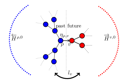
Figure 2. The situation on the binary tree $\mathbb{T}^{2}$. The choice of $v$ induces a splitting of $\mathbb{T}^{d}$ into the blue $d$-ary subtree rooted at $\rho$ and the red $d$-ary subtree of rooted at $v$. The tail-measurable random variables $\overleftarrow{H}^{\rho,0}$ and $\overrightarrow{H}^{v,0}$ are the limits of spherical averages in the past (the future, resp.). Finally, the map $l_{v}$ interchanges the roles of the past and the future.

Hence, taking the $\nu$-a.s.-limit $r\rightarrow\infty$ on both sides of the equation (3.30) leads to

$$H^{\rho,0}=\frac{d}{d+1}\overleftarrow{H}^{\rho,0}+\frac{1}{d+1}\overrightarrow{H}^{v,0}+\frac{1}{d+1}{\eta_{(\rho,v)}}$$ (3.32)

Now consider the joint distribution of $(\sigma_{\rho},\sigma_{v})$ and of $(\sigma_{v},\sigma_{\rho})$. We have for any $s,t\in\mathbb{Z}$

$$\begin{split}\mu^{H}(\sigma_{\rho}=t,\ \sigma_{v}=s)&=\mu^{H}\left(\sigma_{\rho}=t,\ \eta_{(\rho,v)}=s-t\right)\\ \mu^{H}(\sigma_{v}=t,\ \sigma_{\rho}=s)&=\mu^{H}\left(\sigma_{v}=t,\ \eta_{(\rho,v)}=-(s-t)\right).\end{split}$$ (3.33)

From the Expression 2.9 for the single-site marginals of $\sigma_{\rho}$ and $\sigma_{v}$, respectively, of the pinned Gibbs measure $\mu^{H}$ and the decomposition (3.32) of $H^{\rho,0}$ we obtain

$$\begin{split}\mu^{H}(\sigma_{\rho}=t,\ \sigma_{v}=s)&=\nu\left(\lfloor\frac{d}{d+1}\overleftarrow{H}^{\rho,0}+\frac{1}{d+1}\overrightarrow{H}^{v,0}+\frac{s-t}{d+1}\rfloor=-t,\ \eta_{(\rho,v)}=s-t\right)\\ \mu^{H}(\sigma_{v}=t,\ \sigma_{\rho}=s)&=\nu\left(t-s-\lfloor\frac{d}{d+1}\overleftarrow{H}^{(\rho,0)}+\frac{1}{d+1}\overrightarrow{H}^{(v,0)}+\frac{t-s}{d+1}\rfloor=t,\ \eta_{(\rho,v)}=t-s\right).\end{split}$$ (3.34)

Set $Z:=\frac{d}{d+1}\overleftarrow{H}^{\rho,0}+\frac{1}{d+1}\overrightarrow{H}^{v,0}$ and for fixed $t,b\in\mathbb{Z}$ let $s:=s(b):=t+b(d+1)$. Then we have

$$\begin{split}\mu^{H}(\sigma_{\rho}=s,\ \sigma_{v}=t)&=\nu\left(\lfloor Z+a\rfloor=-t,\ \eta_{(\rho,v)}=b(d+1)\right)\\ \mu^{H}(\sigma_{v}=s,\ \sigma_{\rho}=t)&=\nu\left(-b(d+1)-\lfloor Z-b\rfloor=t,\ \eta_{(\rho,v)}=-b(d+1)\right),\end{split}$$ (3.35)

which implies

$$\begin{split}\mu^{H}(\sigma_{\rho}=s,\ \sigma_{v}=t)&=\nu\left(\lfloor Z\rfloor=-t-b,\ \eta_{(\rho,v)}=b(d+1)\right)\\ \mu^{H}(\sigma_{v}=s,\ \sigma_{\rho}=t)&=\nu\left(\lfloor Z\rfloor=-t-bd,\ \eta_{(\rho,v)}=-b(d+1)\right).\end{split}$$ (3.36)

Free state: First consider the case of $\nu$ being the free state of i.i.d.-increments, where the random variable $Z$ is independent of $\eta_{(\rho,v)}$, because of prescribing the height $0$ at $\rho$ (at $v$, resp.) in (3.31). Now we will lead the assumption that $\mu^{H}(\sigma_{\rho}=s,\ \sigma_{v}=t)$ coincides with $\mu^{H}(\sigma_{\rho}=t,\ \sigma_{v}=s)$ for all $s,t\in\mathbb{Z}$ to a contradiction. Then using independence of $Z$ and $\eta_{(\rho,v)}$ and symmetry of the distribution of $\eta_{(\rho,v)}$ the system (3.36) implies that

$$\nu\left(\lfloor Z\rfloor+t=-b\right)=\nu\left(\lfloor Z\rfloor+t=-bd\right)\quad\text{for all }b\in\mathbb{Z}.$$ (3.37)

In particular the sequence $(\nu\left(\lfloor Z\rfloor+t=-bd^{n}\right))_{d\in\mathbb{N}}$ is constant which contradicts the fact that the probability mass function of the discrete random variable $\lfloor Z\rfloor+t$ must be summable. Hence, $\mu^{H}$ cannot be invariant under the translations of the tree.

Hidden Ising model: In case of the hidden Ising model we may further condition (3.36) on the $\mod-2$ spin values at $\rho$ and $v$ to obtain conditional independence between $Z$ and $\eta_{(\rho,v)}$ and afterwards integrate out the outer conditioning. More precisely, assume that $d$ is even (the case of $d$ odd is completely analogous by restricting to odd values of $a$) and restrict to even values of $b$. Then $b(d+1)$ is an even number, so in (3.36) the internal fuzzy chain must coincide at $\rho$ and $v$ to have an increment in class $\bar{0}$. Hence, assuming that $\mu^{H}(\sigma_{\rho}=s,\ \sigma_{v}=t)$ coincides with $\mu^{H}(\sigma_{\rho}=t,\ \sigma_{v}=s)$ for all $s,t\in\mathbb{Z}$ we obtain from (3.36) by taking total expectation

$$\begin{split}&\nu\left(\lfloor Z\rfloor=-t-b,\ \eta_{(\rho,v)}=b(d+1)\mid\bar{\sigma}_{\rho}=\bar{\sigma}_{v}=\bar{0}\right)\bar{\mu}(\bar{\sigma}_{\rho}=\bar{\sigma}_{v}=\bar{0})\cr&\quad+\nu\left(\lfloor Z\rfloor=-t-b,\ \eta_{(\rho,v)}=b(d+1)\mid\bar{\sigma}_{\rho}=\bar{\sigma}_{v}=\bar{1}\right)\bar{\mu}(\bar{\sigma}_{\rho}=\bar{\sigma}_{v}=\bar{1})\cr&=\nu\left(\lfloor Z\rfloor=-t-bd,\ \eta_{(\rho,v)}=-b(d+1)\mid\bar{\sigma}_{\rho}=\bar{\sigma}_{v}=\bar{0}\right)\bar{\mu}(\bar{\sigma}_{\rho}=\bar{\sigma}_{v}=\bar{0})\cr&\quad+\nu\left(\lfloor Z\rfloor=-t-bd,\ \eta_{(\rho,v)}=-b(d+1)\mid\bar{\sigma}_{\rho}=\bar{\sigma}_{v}=\bar{1}\right)\bar{\mu}(\bar{\sigma}_{\rho}=\bar{\sigma}_{v}=\bar{1})\quad\text{ for all }b\in 2\mathbb{Z}.\end{split}$$

Now, conditional independence of $Z$ and $\eta_{(\rho,v)}$, symmetry of the (conditional) distribution of $\eta_{(\rho,v)}$ and the fact that the conditional distribution of $\eta_{(\rho,v)}$ depends only on the height-increment of the fuzzy chain lead to

$$\begin{split}&\nu\left(\lfloor Z\rfloor+t=-b\mid\bar{\sigma}_{\rho}=\bar{\sigma}_{v}=\bar{0}\right)\bar{\mu}(\bar{\sigma}_{\rho}=\bar{\sigma}_{v}=\bar{0})\cr&\quad+\nu\left(\lfloor Z\rfloor+t=-b\mid\bar{\sigma}_{\rho}=\bar{\sigma}_{v}=\bar{1}\right)\bar{\mu}(\bar{\sigma}_{\rho}=\bar{\sigma}_{v}=\bar{1})\cr&=\nu\left(\lfloor Z\rfloor+t=-bd\mid\bar{\sigma}_{\rho}=\bar{\sigma}_{v}=\bar{0}\right)\bar{\mu}(\bar{\sigma}_{\rho}=\bar{\sigma}_{v}=\bar{0})\cr&\quad+\nu\left(\lfloor Z\rfloor+t=-bd\mid\bar{\sigma}_{\rho}=\bar{\sigma}_{v}=\bar{1}\right)\bar{\mu}(\bar{\sigma}_{\rho}=\bar{\sigma}_{v}=\bar{1})\quad\text{ for all }b\in 2\mathbb{Z}.\end{split}$$

As $d$ is even and $b$ runs through all even integers this again contradicts finiteness of the distribution of $\lfloor Z\rfloor$.

This concludes the proof of Proposition 5. ∎

3.5. The distribution of $H$ is supported on $\mathbb{R}$.

By extending the decomposition argument employed in the proof of Proposition 5 above and combining it with the result of Proposition 4 on absolute continuity of the distribution of $H^{\rho,0}$ we prove the following result on the support of the distribution of $H^{\rho,0}$.

Proposition 6.

Let $\nu$ be the free state (a spatially homogeneous GGM of height-period $2$ with a fuzzy Markov chain $\bar{\mu}$, resp.), $H$ be the height-offset variable which is given by Proposition 1 (Proposition 2, resp.) and $H^{\rho,0}$ the push-forward of $H$ to the gradient field under pinning the height $0$ at $\rho$ as in Definition 2.

Then the smooth Lebesgue-density $f_{H^{\rho,0}}$ given by Proposition 4 is supported on $\mathbb{R}$. More precisely, we have that for every $\delta>0$ there exist some lattice $\mathfrak{R}_{\delta}\subset\mathbb{R}$ of the form $\mathfrak{R}_{\delta}=a+\delta\mathbb{Z}$, where $a\in\mathbb{R}$, such that $f_{H^{\rho,0}}$ is strictly positive on $\mathfrak{R}_{\delta}$.

Proof of Proposition 6.

Fix any radius $r_{1}$, and write for $r$ sufficiently large the splitting into independent parts of the following form

$$\begin{split}&\frac{1}{|W_{r}|}\sum_{v\in W_{r}}\sigma_{v}^{\rho,0}=\frac{1}{|W_{r}|}\sum_{u\in W_{r_{1}}}\sum_{v\in W_{r}(u)}(\sigma_{u}^{\rho,0}+\sigma_{v}^{u,0})\cr\end{split}$$ (3.38)

where we write $W_{r}(u)$ for the part of $W_{r}$ which can be reached by non-intersecting paths starting from $u$ pointing away from the origin. So, this is the part of $W_{r}$ which can be seen from $u$. In particular, $W_{r}(u)$ arises as the boundary of a $d$-ary subtree of depth $r-r_{1}$ rooted at $u$. The last term can be rewritten as

$$\begin{split}&\frac{1}{|W_{r_{1}}|}\sum_{u\in W_{r_{1}}}\sigma_{u}^{\rho,0}+\frac{1}{|W_{r_{1}}|}\sum_{u\in W_{r_{1}}}\Bigl{(}\frac{1}{|W_{r}(u)|}\sum_{v\in W_{r}(u)}\sigma_{v}^{u,0}\Bigr{)}.\cr\end{split}$$ (3.39)

Free measure: First restrict to the case of $\nu$ being the free state. Then the random variables

$$\Bigl{(}\frac{1}{|W_{r}(u)|}\sum_{v\in W_{r}(u)}\sigma_{v}^{u,0}\Bigr{)}_{u\in W_{r}}$$

are independent. Again, apply Proposition 2 to the $d$-ary tree rooted at $u$ (cf. Remark 4) to conclude that as $r$ tends to infinity for fixed $r_{1}$, each of the independent $u$-indexed random variables $\frac{1}{|W_{r}(u)|}\sum_{v\in W_{r}(u)}\sigma_{v}^{u,0}$ converges to a HOV on the $d$-ary tree, anchored at $u$ which we denote by $\overrightarrow{H}^{u,0}$. Hence we have the equation

$$\begin{split}&H^{\rho,0}=\frac{1}{|W_{r_{1}}|}\sum_{u\in W_{r_{1}}}\sigma_{u}^{\rho,0}+\frac{1}{|W_{r_{1}}|}\sum_{u\in W_{r_{1}}}\overrightarrow{H}^{u,0}.\end{split}$$ (3.40)

Note that the two terms in (3.40) are independent. Furthermore, by extending the result of Proposition 4 to the $d$-ary tree (cf. Remark 5) we note that each of the independent random variables $\overrightarrow{H}^{u,0}$ has an infinitely often differentiable Lebesgue density $f_{\overrightarrow{H}^{u,0}}$ which by continuity needs to be positive on some open interval. Hence, the random variable $\frac{1}{|W_{r_{1}}|}\sum_{u\in W_{r_{1}}}\overrightarrow{H}^{u,0}$ has a density that is positive on some $r_{1}$ dependent interval $I_{r_{1}}$. On the other hand, the first term in (3.40) is a discrete random variable with range $\frac{\mathbb{Z}}{|W_{r_{1}}|}$, which follows from the fact that the gradient variables are independent under the free measure and have range $\mathbb{Z}$ by the assumption that $Q(i)>0$ for all $i\in\mathbb{Z}$. Combining these two aspects we conclude that $f_{H^{\rho,0}}$ is positive on the set $\frac{1}{|W_{r_{1}}|}\mathbb{Z}+I_{r_{1}}:=\{s+t\mid s\in\frac{1}{|W_{r_{1}}|}\mathbb{Z},\ t\in I_{r_{1}}\}$. For any given $\delta$ we then choose $r_{1}\in\mathbb{N}$ such that $|W_{r_{1}}|>\frac{1}{\delta}$ and select any $a\in I_{r_{1}}$.

Hidden Ising model: To adapt this strategy of proof to the hidden Ising model we first fix some $\bar{\omega}_{B_{r_{1}}}$ and condition on $\bar{\sigma}_{B_{r_{1}}}=\bar{\omega}_{B_{r_{1}}}$ to obtain an independent family

$$\Bigl{(}\frac{1}{|W_{r}(u)|}\sum_{v\in W_{r}(u)}\sigma_{v}^{u,0,\bar{\omega}_{u}}\Bigr{)}_{u\in W_{r}}.$$

Here, $\sigma_{v}^{u,0,\bar{\omega}_{B_{r_{1}}}}$ is the random variable that maps a gradient configuration drawn from on $\nu(\cdot\mid\bar{\sigma}_{B_{r_{1}}}=\bar{\omega}_{B_{r_{1}}})$ to the absolute height at $v$ obtained from prescribing the height $0$ at $u$. Then, we make use that the statement of Proposition 2 remains true if we replace the Cayley tree rooted at $\rho$ by the $d$-ary tree rooted at the respective $u$ and condition on $\bar{\sigma}_{B_{r_{1}}}=\bar{\omega}_{B_{r_{1}}}$ (cf. Remarks 4) to obtain existence of the $\nu$-a.s. limits

$$\overrightarrow{H}^{u,0,\bar{\omega}_{B_{r_{1}}}}:=\lim_{r\rightarrow\infty}\frac{1}{|W_{r}(u)|}\sum_{v\in W_{r}(u)}\sigma_{v}^{u,0,\bar{\omega}_{B_{r_{1}}}},\quad u\in W_{r_{1}}.$$

Let $H^{\rho,0,\bar{\omega}_{B_{r_{1}}}}$ denote the random variable constructed in Proposition 2 with $\nu(\cdot)$ replaced by $\nu(\cdot\mid\bar{\sigma}_{B_{r_{1}}}=\bar{\omega}_{B_{r_{1}}})$ to arrive at the following analogue of (3.40):

$$\begin{split}&H^{\rho,0,\bar{\omega}_{B_{r_{1}}}}=\frac{1}{|W_{r_{1}}|}\sum_{u\in W_{r_{1}}}\sigma_{u}^{\rho,0,\bar{\omega}_{B_{r_{1}}}}+\frac{1}{|W_{r_{1}}|}\sum_{u\in W_{r_{1}}}\overrightarrow{H}^{u,0,\bar{\omega}_{B_{r_{1}}}}.\end{split}$$ (3.41)

By construction of the hidden Ising model, the two terms in (3.41) are independent under $\nu(\cdot\mid\bar{\sigma}_{B_{r_{1}}}=\bar{\omega}_{B_{r_{1}}})$. Furthermore, by the extension of Proposition 4 in the sense of Remark 5, the second term and the l.h.s of (3.41) have infinitely-often differentiable Lebesgue-densities. Each of the random variables $\sigma_{u}^{\rho,0,\bar{\omega}_{B_{r_{1}}}}$ is the sum of independent gradient variables whose range are either all even integers or all odd integers (depending on the respective conditioning along the edge). For the particular case of the all-zero conditioning $\bar{\omega}_{B_{r_{1}}}=\bar{0}_{B_{r_{1}}}$ the range of the random variable $\frac{1}{|W_{r_{1}}|}\sum_{u\in W_{r_{1}}}\sigma_{u}^{\rho,0,\bar{\omega}_{B_{r_{1}}}}$ includes the $r_{1}$-dependent lattice $\frac{2}{|W_{r_{1}}|}\mathbb{Z}$. Writing

$$f_{H^{\rho,0}}(\cdot)=\sum_{\bar{\omega}_{B_{r_{1}}}\in\mathbb{Z}_{2}^{B_{r_{1}}}}f_{H^{\rho,0,\bar{\omega}_{B_{r_{1}}}}}(\cdot)\,\nu(\bar{\sigma}_{B_{r_{1}}}=\bar{\omega}_{B_{r_{1}}})$$

we can now proceed as in the case of the free measure. ∎

3.6. The pinned measures are no Markov chains and not extreme

A further inspection of the decomposition arguments of the proof of Proposition 6 reveals the following:

Proposition 7.

1. Let $\nu$ be the free state and let $H$ be the height-offset variable which is given by Proposition 1. Then the Gibbs measure $\mu^{H}$ is not a tree-indexed Markov chain. In particular, it is not extreme in the set of all Gibbs measures.

2. Let $\nu$ be a gradient Gibbs measure of height-period $2$ for some fuzzy chain $\bar{\mu}$ and let $H$ be the height-offset variable which is given by Proposition 2. Then the Gibbs measure $\mu^{H}$ is not extreme.

Proof of Proposition 7.

First we prove Statement (a) regarding the free state. Let $v\in\partial\{\rho\}$ and as in the proof of Proposition 5 above consider the splitting

$$H^{\rho,0}=\frac{d}{d+1}\overleftarrow{H}^{\rho,0}+\frac{1}{d+1}\overrightarrow{H}^{v,0}+\frac{1}{d+1}{\eta_{(\rho,v)}}$$

of the limit of averages over the $r$-spheres into the respective subgraphs of the past and of future (cf. Equation (3.32) and Figure 2). Further abbreviate

$$X:=\frac{d}{d+1}\overleftarrow{H}^{\rho,0}\quad\text{and}\quad Y:=\frac{1}{d+1}\overrightarrow{H}^{v,0}.$$

We will now draw the assumption that the associated $H$-pinned Gibbs measure $\mu^{H}$ is a Markov chain to a contradiction. More precisely, we will show that

$$\mu^{H}(\sigma_{v}=\cdot\mid\mathcal{F}_{(-\infty,\rho v]})=\mu^{H}(\sigma_{v}=\cdot\mid\sigma_{\rho},\,X)\quad\mu^{H}-a.s.$$ (3.42)

necessarily depends in a non-trivial way on $X$. In words, the distribution of the spin at $v$ recalls the part in the infinite past of the HOV $H$. Note that the definition of a tree-indexed Markov chain involves a $\mu^{H}$-almost sure statement, hence we will take extra care to condition only on events with positive mass. As we consider the case of $\nu$ being the free state of i.i.d.-increments, the gradient spin along the edge $(\rho,v)$ and the random variables $X$ and $Y$ are independent.

Compute for any integers $t$ and $t^{\prime}$ the conditional probability of $\sigma_{v}^{\prime}=t^{\prime}$ given $\sigma_{\rho}=t$ and $X\in A$, where $A$ is any Borel set with $\nu(X\in A)>0$. Then the single-site marginals representation (2.9) and independence lead to

$$\begin{split}&\mu^{H}(\sigma_{v}=t^{\prime}\mid\sigma_{\rho}=t,X\in A)\cr&=\frac{\nu\left(\,\lfloor{X+Y+\frac{\eta_{(\rho,v)}}{d+1}}\rfloor=-t,\,\eta_{(\rho,v)}-\lfloor{X+Y+\frac{\eta_{(\rho,v)}}{d+1}}\rfloor=t^{\prime}\,,X\in A\right)}{\nu\left(\,\lfloor{X+Y+\frac{\eta_{(\rho,v)}}{d+1}}\rfloor=-t\,,X\in A\right)}\cr&=\nu(\eta_{(\rho,v)}=t^{\prime}-t)\cdot\frac{\nu\left(\,\lfloor{X+Y+\frac{t^{\prime}-t}{d+1}}\rfloor=t,\ X\in A\right)}{\nu\left(\,\lfloor{X+Y+\frac{\eta_{(\rho,v)}}{d+1}}\rfloor=t,X\in A\right)}.\end{split}$$ (3.43)

Now assume that $\mu^{H}(\sigma_{v}=t^{\prime}\mid\sigma_{\rho}=t,X\in A)$ would not depend on $A$. Then the second factor of the last expression in (3.43) would be some function $C(t,t^{\prime})$ which does not depend on $A$. So,

$$\begin{split}C(t,t^{\prime})=\frac{\nu\left(\,\lfloor{X+Y+\frac{t^{\prime}-t}{d+1}}\rfloor=t,\ X\in A\right)}{\nu\left(\,\lfloor{X+Y+\frac{\eta_{(\rho,v)}}{d+1}}\rfloor=t,X\in A\right)}\quad\text{for all }t,t^{\prime}\in\mathbb{Z}.\end{split}$$ (3.44)

Now consider (3.44) for $t^{\prime},t^{\prime\prime}\in\mathbb{Z}$ and take the quotient of both expressions to obtain

$$\begin{split}\tilde{C}(t,t^{\prime},t^{\prime\prime}):=\frac{C(t,t^{\prime})}{C(t,t^{\prime\prime})}=\frac{\nu\left(\,\lfloor{X+Y+\frac{t^{\prime}-t}{d+1}}\rfloor=t,\ X\in A\right)}{\nu\left(\,\lfloor{X+Y+\frac{t^{\prime\prime}-t}{d+1}}\rfloor=t,\ X\in A\right)}.\end{split}$$ (3.45)

By Proposition 6 applied to the $d$-ary tree instead of the Cayley tree, there is some (arbitrarily small) $a\in\mathbb{R}$ such that the Lebesgue-density $f_{X}$ is positive on $a+\mathbb{Z}$. For $h\in\mathbb{Z}+a$ and $\varepsilon>0$ specify to $A:=A_{h,\varepsilon}:=[h,h+\varepsilon]$ and further set $t^{\prime}:=t+d+1$ and $t^{\prime\prime}:=t$. Then employ the fact that $X$ and $Y$ have smooth Lebesgue densities $f_{X}$ and $f_{Y}$ to get from (3.45) to

$$\begin{split}\hat{C}(t):=\tilde{C}(t,t+d+1,t)=\frac{\tfrac{1}{\varepsilon}\int_{A_{h,\varepsilon}}f_{X}(x)\lambda(dx)\int f_{Y}(y)\lambda(dy)1_{\{\lfloor x+y\rfloor=t-1\}}}{\tfrac{1}{\varepsilon}\int_{A_{h,\varepsilon}}f_{X}(x)\lambda(dx)\int f_{Y}(y)\lambda(dy)1_{\{\lfloor x+y\rfloor=t\}}}\end{split}$$ (3.46)

By the continuity lemma (cf. [17, Theorem 6.27]) the function

$$A_{h,\varepsilon}\ni x\mapsto f_{X}(x)\int f_{Y}(y)\lambda(dy)1_{\{\lfloor x+y\rfloor=t-1\}}\in\mathbb{R}$$

is continuous and hence every $x\in A_{h,\varepsilon}$ is a Lebesgue point. From the Lebesgue differentiation theorem we thus deduce

$$\lim_{\varepsilon\rightarrow 0}\tfrac{1}{\varepsilon}f_{X}(x)\lambda(dx)\int f_{Y}(y)\lambda(dy)1_{\{\lfloor x+y\rfloor=t-1\}}=f_{X}(h)\int f_{Y}(y)\lambda(dy)1_{\{\lfloor h+y\rfloor=t-1\}}.$$

As the density $f_{X}$ is in particular positive on $a+\mathbb{Z}$, we may apply the same reasoning to the denominator in (3.46). Thus we obtain

$$\hat{C}(t)=\frac{\nu(\lfloor Y+h\rfloor=t-1)}{\nu(\lfloor Y+h\rfloor=t)}\quad\text{ for all }h\in a+\mathbb{Z}.$$ (3.47)

In particular,

$$\hat{C}(t)=\frac{\nu(\lfloor Y+a-t\rfloor=l-1)}{\nu(\lfloor Y+a-t\rfloor=l)}\quad\text{ for all }l\in\mathbb{Z}.$$ (3.48)

This is a contradiction to the fact that the probability mass function of $\lfloor Y+a-t\rfloor$ is summable. Hence, we have proven that for the free state $\nu^{free}$ the pinned Gibbs measure $\mu^{H}$ cannot be a tree-indexed Markov chain.

Now we prove statement (b), which says that a gradient Gibbs measure of height-period $2$ cannot be extreme in the set of Gibbs measures. Following the framework of Sheffield ([25, Lemma 8.4.2]) and its application to the graph-homomorphism model by Lammers and Toninelli [21, Remark 2.7] we define the height-offset spectrum of the HOV $H$ for a GGM $\nu$ as the distribution of $H$ w.r.t. to the Gibbs measure $\mu^{H}$. By definition, $H$ is tail-measurable w.r.t. the absolute heights. Furthermore, by construction of $\mu^{H}$, the height-offset spectrum is described by the distribution of $H(\sigma^{x,s})-\lfloor H(\sigma^{x,s})\rfloor$ under $\nu$ for any $x\in V$ and $s\in\mathbb{Z}$. Now consider the set-up of Proposition 2 where $H$ is constructed as a limit of averages over spheres. Proposition 4 above guarantees that the distribution $H^{\rho,0}$ under $\nu$ is absolutely continuous w.r.t. Lebesgue measure. In particular, $H(\sigma^{x,s})-\lfloor H(\sigma^{x,s})\rfloor$ is not a Dirac measure. Hence, from the equivalence of extremality of Gibbs measures and their tail-triviality ([13, Proposition 7.9]) we conclude that $\mu^{H}$ is not extreme in the set of Gibbs measures. ∎

4. Applications

For the sake of illustration let us provide explicit expressions for the following frequently studied examples.

4.1. SOS model

The SOS model is described by the interaction $U(j)=|j|$, which corresponds to the transfer operator $Q$ defined by $Q_{\beta}^{\text{SOS}}(j)=\exp(-\beta|j|)$. From this we obtain the single-gradient moment generating function

$$\hat{\psi}^{free}(s)=\frac{(\exp(\beta)-1)^{2}}{\exp(2\beta)-2\exp(\beta)\cosh(s)+1},\quad s\in[0,\beta),$$ (4.1)

with a singularity at $s=\beta$. Hence, all results of Theorems 2 and 3 can be made explicit and in particular we have the exponential concentration of the marginal at the root of the free measure pinned at infinity, with any exponent smaller $\beta(d+1)$.

4.2. Discrete Gaussian model

The discrete Gaussian model is described by the interaction $U(j)=j^{2}$, which corresponds to the transfer operator $Q$ defined by $Q_{\beta}^{\text{Gau\ss}}(j)=\exp(-\beta j^{2})$. From this we obtain the single-gradient Laplace-transform

$$\hat{\psi}^{free}(s)=\exp\left(\frac{s^{2}}{2\beta}\right)\frac{\sum_{j\in\mathbb{Z}}\exp\left(-\frac{\beta}{2}(j-\frac{s}{\beta})^{2}\right)}{\sum_{j\in\mathbb{Z}}\exp(-\frac{\beta}{2}j^{2})}$$ (4.2)

which gives us super-exponential concentration for the marginal.

5. Appendix

5.1. Proof of Theorem 1

Proof of Theorem 1.

Let $\emptyset\neq\Lambda\subset\Delta\Subset V$ and $\tilde{\omega}\in\Omega$ such that $\mu(\sigma_{\Delta\setminus\Lambda}=\tilde{\omega}_{\Delta\setminus\Lambda})\neq 0$. Further choose any $x\in\partial\Lambda$. Then, using Definition 1 and going over to gradients on the complement of $\partial\Lambda$ in the next step we have $\nu$-a.s.

$$\begin{split}&\mu(\sigma_{\Lambda\cup\partial\Lambda}=\tilde{\omega}_{\Lambda\cup\partial\Lambda}\mid\sigma_{\Delta\setminus\Lambda}=\tilde{\omega}_{\Delta\setminus\Lambda})\cr&=\nu((\sigma^{x,0})_{\Lambda\cup\partial\Lambda}=\tilde{\omega}_{\Lambda\cup\partial\Lambda}+\lfloor H(\sigma^{x,0})\rfloor\mid(\sigma^{x,0})_{\Delta\setminus\Lambda}=\tilde{\omega}_{\Delta\setminus\Lambda}+\lfloor H(\sigma^{x,0})\rfloor)\cr&=\nu(\eta_{\Lambda\cup\partial\Lambda}=(\nabla\tilde{\omega})_{\Lambda\cup\partial\Lambda},\,(\sigma^{x,0})_{\partial\Lambda}=\tilde{\omega}_{\partial\Lambda}+\lfloor H(\sigma^{x,0})\rfloor\cr&\qquad\mid\eta_{\Delta\setminus\Lambda}=(\nabla\tilde{\omega})_{\Delta\setminus\Lambda},\,(\sigma^{x,0})_{\partial\Lambda}=\tilde{\omega}_{\partial\Lambda}+\lfloor H(\sigma^{x,0})\rfloor)\cr&=\nu(\eta_{\Lambda\cup\partial\Lambda}=(\nabla\tilde{\omega})_{\Lambda\cup\partial\Lambda}\mid\eta_{\Delta\setminus\Lambda}=(\nabla\tilde{\omega})_{\Delta\setminus\Lambda},\,(\sigma^{x,0})_{\partial\Lambda}-\lfloor H(\sigma^{x,0})\rfloor=\tilde{\omega}_{\partial\Lambda}).\end{split}$$ (5.1)

In the last line we used the elementary relation that the new probability of $A\cap B$ conditional on $B\cap C$ is the probability of $A$ conditional on $B\cap C$.
Note that the conditioning contains information on the gradient field outside $\Lambda$ as well as information on the relative heights at the boundary $\partial\Lambda$ together with the pinning prescribed by $H$. Hence, it is possible to equivalently describe the conditioning in terms of pinning at the point $x$ and the relative heights at the boundary. More precisely, we have

$$\{(\sigma^{x,0})_{\partial\Lambda}-\lfloor H(\sigma^{x,0})\rfloor=\tilde{\omega}_{\partial\Lambda}\}=\{\lfloor H(\sigma^{x,0})\rfloor=-\tilde{\omega}_{x}\}\cap\{[\eta]_{\partial\Lambda}=[\nabla\tilde{\omega}]_{\partial\Lambda}\}$$ (5.2)

By tail-measurability (with respect to the heights) of $H$ the event $\{\lfloor H(\sigma^{x,0})\rfloor=-\tilde{\omega}_{x}\}$ is measurable with respect to $\mathcal{T}^{\nabla}_{\Lambda}$. Indeed, pinning the height $0$ at $x$ together with the relative heights at $\partial\Lambda$ and the gradient field outside $\Lambda$ provides all information on $(\sigma^{x,0})_{\Lambda^{c}}$. Now employ the fact that the conditional distribution of the gradient field inside $\Lambda\cup\partial\Lambda$ under $\nu$ given $\mathcal{T}_{\Lambda}^{\nabla}$ is already measurable with respect to the relative heights at the boundary to conclude

$$\begin{split}&\nu(\eta_{\Lambda\cup\partial\Lambda}=(\nabla\tilde{\omega})_{\Lambda\cup\partial\Lambda}\mid\eta_{\Delta\setminus\Lambda}=(\nabla\tilde{\omega})_{\Delta\setminus\Lambda},\,(\sigma^{x,0})_{\partial\Lambda}-\lfloor H(\sigma^{x,0})\rfloor=\tilde{\omega}_{\partial\Lambda})\cr&=\nu(\eta_{\Lambda\cup\partial\Lambda}=(\nabla\tilde{\omega})_{\Lambda\cup\partial\Lambda}\mid[\eta]_{\partial\Lambda}=[\nabla\tilde{\omega}]_{\partial\Lambda})\end{split}$$ (5.3)

Taking into account the DLR-equation for the gradient Gibbs measure $\nu$ hence allows to rewrite the last expression of (5.1) as

$$\begin{split}&\nu(\eta_{\Lambda\cup\partial\Lambda}=(\nabla\tilde{\omega})_{\Lambda\cup\partial\Lambda}\mid\eta_{\Delta\setminus\Lambda}=(\nabla\tilde{\omega})_{\Delta\setminus\Lambda},\,(\sigma^{x,0})_{\partial\Lambda}-\lfloor H(\sigma^{x,0})\rfloor=\tilde{\omega}_{\partial\Lambda})\cr&=\gamma^{\nabla}(\eta_{\Lambda\cup\partial\Lambda}=(\nabla\tilde{\omega})_{\Lambda\cup\partial\Lambda}\mid\eta=\nabla\tilde{\omega},\,[\eta]_{\partial\Lambda}=[\nabla\tilde{\omega}]_{\partial\Lambda})\cr&=\gamma(\sigma_{\Lambda}=\tilde{\omega}_{\Lambda}\mid\tilde{\omega}),\end{split}$$

which in combination with 5.1 shows that $\mu$ satisfies the DLR-equation. This finishes the proof of Theorem 1. ∎

Declarations

Data Availability: Data sharing is not applicable to this article. The plots in Figures 1 and 2 have been generated within a separate .tex-file using the TikZ-package.
Competing interests: The authors have no competing interests to declare that are relevant to the content of this article.

References

• [1] Alberto Abbondandolo, Florian Henning, Christof Külske and Pietro Majer “Infinite-volume states with irreducible localization sets for gradient models on trees” In J. Stat. Phys. 191.6, 2024, pp. Paper No. 63, 35 DOI: 10.1007/s10955-024-03278-9
• [2] Roland Bauerschmidt, Jiwon Park and Pierre-Franγois Rodriguez “The Discrete Gaussian model, II. Infinite-volume scaling limit at high temperature” In Preprint, 2022 arXiv:2202.02287
• [3] Nishant Chandgotia, Ron Peled, Scott Sheffield and Martin Tassy “Delocalization of uniform graph homomorphisms from $\mathbb{Z}^{2}$ to $\mathbb{Z}$ In Comm. Math. Phys. 387.2, 2021, pp. 621–647 DOI: 10.1007/s00220-021-04181-0
• [4] Loren Coquille, Christof Külske and Arnaud Le Ny “Extremal inhomogeneous Gibbs states for SOS-models and finite-spin models on trees” In J. Stat. Phys. 190.4, 2023, pp. Paper No. 71, 26 DOI: 10.1007/s10955-023-03081-y
• [5] Codina Cotar and Christof Külske “Uniqueness of gradient Gibbs measures with disorder” In Probability Theory and Related Fields 162.3, 2015, pp. 587–635 DOI: 10.1007/s00440-014-0580-x
• [6] Paul Dario, Matan Harel and Ron Peled “Random-field random surfaces” In Probab. Theory Related Fields 186.1-2, 2023, pp. 91–158 DOI: 10.1007/s00440-022-01179-0
• [7] Jean-Dominique Deuschel, Giambattista Giacomin and Dmitry Ioffe “Large deviations and concentration properties for $\nabla\phi$ interface models” In Probab. Theory Related Fields 117.1, 2000, pp. 49–111 DOI: 10.1007/s004400050266
• [8] Jean-Dominique Deuschel and Pierre-Franγ cois Rodriguez “A Ray-Knight theorem for $\nabla\phi$ interface models and scaling limits” In Probab. Theory Related Fields 189.1-2, 2024, pp. 447–499 DOI: 10.1007/s00440-024-01275-3
• [9] Hugo Duminil-Copin et al. “Logarithmic variance for the height function of square-ice” In Comm. Math. Phys. 396.2, 2022, pp. 867–902 DOI: 10.1007/s00220-022-04483-x
• [10] Aernout C. D. Enter and Christof Külske “Nonexistence of Random Gradient Gibbs Measures in Continuous Interface Models in d = 2” In Ann. Appl. Probab. 18.1 Institute of Mathematical Statistics, 2008, pp. 109–119 DOI: 10.1214/07-AAP446
• [11] William Feller “An introduction to probability theory and its applications. Vol. II” John Wiley & Sons, Inc., New York-London-Sydney, 1971, pp. xxiv+669
• [12] T. Funaki and H. Spohn “Motion by Mean Curvature from the Ginzburg-Landau Interface Model” In Comm. Math. Phys. 185.1, 1997, pp. 1–36 DOI: 10.1007/s002200050080
• [13] Hans-Otto Georgii “Gibbs measures and phase transitions” 9, de Gruyter Studies in Mathematics Walter de Gruyter & Co., Berlin, 2011, pp. xiv+545 DOI: 10.1515/9783110250329
• [14] Florian Henning and Christof Külske “Coexistence of localized Gibbs measures and delocalized gradient Gibbs measures on trees” In Ann. Appl. Probab. 31.5, 2021, pp. 2284–2310 DOI: 10.1214/20-aap1647
• [15] Florian Henning and Christof Külske “Existence of gradient Gibbs measures on regular trees which are not translation invariant” In Ann. Appl. Probab. 33.4, 2023, pp. 3010–3038 DOI: 10.1214/22-aap1883
• [16] Florian Henning, Christof Külske, Arnaud Le Ny and Utkir A. Rozikov “Gradient Gibbs measures for the SOS-model with countable values on a Cayley tree” In Electron. J. Probab. 24, 2019 DOI: 10.1214/19-EJP364
• [17] Achim Klenke “Probability theory”, Universitext Springer, London, 2020, pp. xiv+716 DOI: 10.1007/978-3-030-56402-5
• [18] Christof Külske and Philipp Schriever “Gradient Gibbs measures and fuzzy transformations on trees” In Markov Process. Related Fields 23.4, 2017, pp. 553–590 URL: https://www.ruhr-uni-bochum.de/imperia/md/content/mathematik/kuelske/grad-gibbs-fuzzy-transf-tree.pdf
• [19] Piet Lammers “Height function delocalisation on cubic planar graphs” In Probab. Theory Related Fields 182.1-2, 2022, pp. 531–550 DOI: 10.1007/s00440-021-01087-9
• [20] Piet Lammers and Sébastien Ott “Delocalization and absolute-value-FKG in the solid-on-solid model” In Probability Theory and related fields, 2023 DOI: 10.1007/s00440-023-01202-y
• [21] Piet Lammers and Fabio Toninelli “Height function localisation on trees” In Combinatorics, Probability and Computing Cambridge University Press, 2023, pp. 1–15 DOI: 10.1017/S0963548323000329
• [22] A. Mielke “Formulation of thermoelastic dissipative material behavior using GENERIC” In Continuum Mechanics and Thermodynamics 23.3 Springer, 2011, pp. 233–256
• [23] Hironobu Sakagawa “Maximum of the Gaussian interface model in random external fields” In J. Stat. Phys. 191.8, 2024, pp. Paper No. 94, 27 DOI: 10.1007/s10955-024-03309-5
• [24] Martin Sellke “Localization of Random Surfaces with Monotone Potentials and an FKG-Gaussian Correlation Inequality” In Preprint, 2024 arXiv:2402.18737
• [25] Scott Sheffield “Random surfaces”, Astérisque 304 Société mathématique de France, 2005 URL: http://www.numdam.org/item/AST_2005__304__R1_0
• [26] Yvan Velenik “Localization and delocalization of random interfaces” In Probab. Surv. 3, 2006, pp. 112–169 DOI: 10.1214/154957806000000050
• [27] Stan Zachary “Countable state space Markov random fields and Markov chains on trees” In Ann. Probab. 11.4, 1983, pp. 894–903 DOI: 10.1214/aop/1176993439