$H\to ZZ$ as a double-slit experiment

Abstract

The decay $H\to ZZ\to 4\ell$, with $\ell=e,\mu$, can be used to test quantum interference in analogy to the famous double-slit experiment. The observations corresponding to ‘covering a slit’ can be extracted from data in the $ee\mu\mu$ channel, while the observations when both ‘slits’ are open, which include the interference, are measured in the $4e/4\mu$ channels. Furthermore, this process offers a unique opportunity to investigate identical-particle effects at high energies, and provide the first evidence of identical-particle behaviour for muons. Sensitivity at the $4\sigma$ level could be achieved at the high-luminosity upgrade of the Large Hadron Collider.

Quantum mechanics (QM) is essential for our understanding of Nature. When performing tests of QM at high energies we are probing its boundaries and thereby extending the range in which it is known to be a correct description of Nature. At present there is no compelling alternative to extend QM as formulated in the early 20${}^{\text{th}}$ century; however, this fact does not diminish the importance of performing tests at high energies and under extreme conditions, where QM might start to break down. Quantum mechanics underlies quantum field theory, which successfully describes all particle interactions via the Standard Model. Therefore, all production and decay processes observed at the Large Hadron Collider (LHC) are quantum in nature. Nonetheless, inherently quantum tests, such as those of entanglement already performed [1, 2, 3], remain of significant interest to probe the foundations of quantum mechanics at high energy.

In this Letter we consider the Higgs boson decay $H\to ZZ$ in the four-lepton final state, highlighting its role as a novel test of identical-particle effects and quantum interference. Tests of identical-particle effects have already been performed with photons [4] and electrons [5]. The $H\to ZZ\to 4\ell$ process with $\ell=e,\mu$ not only provides a further test for electrons at higher energies, but, remarkably, the first test for muons, for which experimental evidence of their identical-particle behaviour is lacking. Moreover, $H\to ZZ\to 4\ell$ demonstrates quantum interference, in a way analogous to the classic double-slit experiment.

There are several magnitudes that differ between the decays into identical and distinguishable fermions, for example, the total decay width and the invariant mass distributions. In addition to those, some angular correlations exhibit striking differences. We will first set up our framework to study the angular correlations in the decay, to later discuss how to test interference and identical-particle effects.

Framework. For the sake of clarity we first discuss the $ee\mu\mu$ final state, where the particles are distinguishable and the two intermediate bosons can be uniquely identified by the flavour of their decay products. We will work in the helicity basis, a moving reference system with vectors $(\hat{r},\hat{n},\hat{k})$ defined as follows [6]:

• $\hat{k}$ is taken in the direction of one of the $Z$ bosons in the Higgs rest frame; we select the one with largest invariant mass and label it as $Z_{1}$, with decay products $\ell_{1}^{+}$, $\ell_{1}^{-}$. The other boson is labelled as $Z_{2}$, with decay products $\ell_{2}^{+}$, $\ell_{2}^{-}$.

• $\hat{r}$ is defined as $\hat{r}=\mathrm{sign}(\cos\theta)(\hat{p}_{p}-\cos\theta\hat{k})/\sin\theta$, with $\hat{p}_{p}=(0,0,1)$ the direction of one proton in the laboratory frame, and $\cos\theta=\hat{k}\cdot\hat{p}_{p}$.

• $\hat{n}$ is taken orthogonal, $\hat{n}=\hat{k}\times\hat{r}$.

The angular orientation of the decay products can be specified by the polar and azimuthal angles $\Omega_{1}=(\theta_{1},\phi_{1})$ and $\Omega_{2}=(\theta_{2},\phi_{2})$ of the negative lepton momenta in the rest frame of the parent $Z$ boson, measured in the $(\hat{r},\hat{n},\hat{k})$ reference system. The four-dimensional decay angular distribution reads [7]

$$\frac{1}{\sigma}\frac{d\sigma}{d\Omega_{1}d\Omega_{2}} = \frac{1}{(4\pi)^{2}}\left[1+a_{LM}^{1}Y_{L}^{M}(\Omega_{1})+a_{LM}^{2}Y_{L}^{M}(\Omega_{2})\right.$$ (1)

$$\left.+c_{L_{1}M_{1}L_{2}M_{2}}Y_{L_{1}}^{M_{1}}(\Omega_{1})Y_{L_{2}}^{M_{2}}(\Omega_{2})\right]\,,$$

with $Y_{L}^{M}$ the usual spherical harmonics, and implicit sum over repeated indices. In the $ee\mu\mu$ final state with distinguishable particles the constants $a_{LM}^{1,2}$, $c_{L_{1}M_{1}L_{2}M_{2}}$ are related to the coefficients in the spin density operator $\rho_{S_{1}S_{2}}$ for the two $Z$ bosons [7]. Specifically, this operator can be written as an expansion in irreducible tensors $T^{L}_{M}$,

$$\rho_{S_{1}S_{2}} = \frac{1}{9}\left[\mathbb{1}_{3}\otimes\mathbb{1}_{3}+A^{1}_{LM}T^{L}_{M}\otimes\mathbb{1}_{3}+A^{2}_{LM}\mathbb{1}_{3}\otimes T^{L}_{M}\right.$$ (2)

$$\left.+C_{L_{1}M_{1}L_{2}M_{2}}\ T^{L_{1}}_{M_{1}}\otimes T^{L_{2}}_{M_{2}}\right]\,,$$

with constants $A_{LM}^{1,2}$, $C_{L_{1}M_{1}L_{2}M_{2}}$. The precise definition of $T^{L}_{M}$ is not relevant here, and can be found e.g. in Ref. [7]. For leptonic $Z$ decays one has $a_{LM}^{1,2}=B_{L}A_{LM}^{1,2}$, $c_{L_{1}M_{1}L_{2}M_{2}}=B_{L_{1}}B_{L_{2}}C_{L_{1}M_{1}L_{2}M_{2}}$, with $B_{1}=-\sqrt{2\pi}\eta_{\ell}$, $B_{2}=\sqrt{2\pi/5}$, and

$$\eta_{\ell}=\frac{1-4s_{W}^{2}}{1-4s_{W}^{2}+8s_{W}^{4}}\simeq 0.13\,,$$ (3)

$s_{W}$ being the sine of the weak angle [8]. The $\eta_{\ell}$ factor suppresses the coefficients of spherical harmonics with $L=1$ in the distribution (1), especially $c_{1010}$ and $c_{111-1}$.

In $4e/4\mu$ final states with identical particles there are two possible pairings between opposite-sign leptons. (Each pairing corresponds to one of the two tree-level $H\to ZZ\to 4\ell$ Feynman diagrams, related by exchange of identical particles.) Let us consider one such pairing and label with a common subindex the leptons in the same pair, $(\ell_{1}^{+},\ell_{1}^{-})$, $(\ell_{2}^{+},\ell_{2}^{-})$. One can then define the two $Z$ bosons by their momenta, $p_{Z_{1}}=p_{\ell_{1}^{+}}+p_{\ell_{1}^{-}}$, $p_{Z_{2}}=p_{\ell_{2}^{+}}+p_{\ell_{2}^{-}}$. And, as before, label as $Z_{1}$ the one with largest invariant mass. The reference system is then constructed as described for distinguishable particles, and likewise the four-dimensional decay distribution has the form (1). However, the numerical values of the coefficients $a_{LM}^{1,2}$ and $c_{L_{1}M_{1}L_{2}M_{2}}$ differ from the $ee\mu\mu$ final state. In particular, $c_{111-1}$ and $c_{1010}$ are up to 50 times larger, depending on the phase space region. We will precisely use the value of these coefficients to demonstrate the effects of interference and identical particles.

Probing quantum interference. In the $ee\mu\mu$ final state there is a ‘correct’ pairing of opposite-sign leptons (by flavour), let us label it as ‘A’. The ‘wrong’ pairing is labelled as ‘B’. We can regard each pairing as a ‘slit’, and measure $c_{111-1}$ and $c_{1010}$ in each case. That would be the analogous to covering any of the two slits in the classical experiment. In addition, we can also perform the measurement counting each event twice, one for each pairing. The result obtained is the average of both pairings, which do not interfere.

In the $4e/4\mu$ final states we can also count each event twice, one for each possible pairing. But the results obtained for $c_{111-1}$ and $c_{1010}$ are not the average of pairings A and B, as in the $ee\mu\mu$ channel. In other words, the observation for $4e/4\mu$ is not the sum of the observations for either of the two ‘slits’ in $ee\mu\mu$. This is a clear indication of the interference. In terms of Feynman diagrams, each pairing — or ‘slit’ — can be identified with a diagram, but note that our definitions and method to verify the interference do not rely on an expansion of the amplitude in terms of Feynman diagrams.

This can be illustrated with a Monte Carlo calculation at the parton level. We generate $H\to ZZ\to 4\ell$ at the leading order with MadGraph [10]. For $ee\mu\mu$ we obtain

Pairing A $$c_{111-1}=0.098 c_{1010}=-0.059\,,$$

Pairing B $$c_{111-1}=-1.210 c_{1010}=14.244\,,$$

Both pairings $$c_{111-1}=-0.556 c_{1010}=7.093\,.$$ (4)

As said, the result when counting each event twice is the average of pairings A and B. For $4e/4\mu$ we have

Both pairings $$c_{111-1}=-0.032 c_{1010}=6.232\,,$$ (5)

which is not the average of pairings A and B, and exhibits the interference effect.

The difference between the $4e/4\mu$ and $ee\mu\mu$ channels can also be studied as a function of $m_{Z_{1}}$, which is generally different for each pairing. The results are presented in Fig. 1, in 5 GeV bins. Note that despite the fact that two pairings of a given event may in general lie in different bins, the differential distribution can be used as a probe of quantum interference.

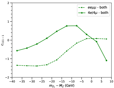
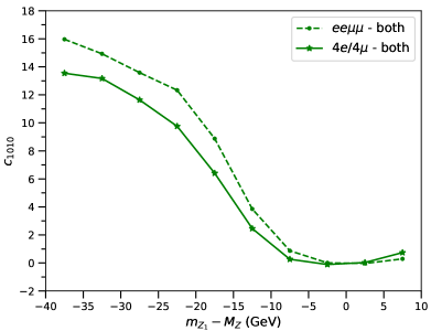
Figure 1: Dependence of the correlation coefficients $c_{111-1}$, $c_{1010}$ on $m_{Z_{1}}$, for $ee\mu\mu$ and $4e/4\mu$ final states, using both pairings of opposite-sign leptons.

Probing identical-particle effects. In order to have a genuine test, one has to apply the same criterion to pair opposite-sign leptons in the $ee\mu\mu$ and $4e/4\mu$ final states and compare some observable, for example the values of $c_{111-1}$, $c_{1010}$ obtained using both pairings. We discuss here some alternatives.

One simple but effective flavour-blind criterion that selects the correct pairing for $ee\mu\mu$ in the vast majority of the events is, among the two possibilities, to choose the one yielding the largest value of $m_{Z_{1}}$. We will denote this criterion as ‘mass pairing’. For low values of $m_{Z_{1}}$, i.e. when both bosons in $H\to ZZ\to ee\mu\mu$ are far from their mass shell, this criterion often fails to select the correct pairing; nevertheless, this phase space region amounts to a small fraction of the decay width. The kinematical distributions of $m_{Z_{1}}$ and $m_{Z_{2}}$ are presented in Fig. 2. The former already provides a good discriminant to test identical-particle effects.

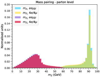
Figure 2: Kinematical distributions of $m_{Z_{1}}$ and $m_{Z_{2}}$, when applying mass pairing of opposite-sign leptons.

To improve the identification in the low-$m_{Z_{1}}$ region a boosted decision tree (BDT) can be trained using as input variables, for each of the two pairings (i) the two invariant masses of opposite-sign lepton pairs, $m_{Z_{1}}$, $m_{Z_{2}}$; (ii) the cosines of the angles between leptons in the same pair, $z_{1}$, $z_{2}$, taking the momenta in the Higgs boson rest frame. We implement this BDT using XGboost [9] with a maximum tree depth of 4, and a maximum of 100 trees, and otherwise default settings. The BDT is trained on the $ee\mu\mu$ final state. For $m_{Z_{1}}\geq 80$ GeV the BDT identifies the correct pairing in more than 99% of the events. The percentage decreases to 85% for $70\leq m_{Z_{1}}\leq 75$ GeV, and drops to 58% for $55\leq m_{Z_{1}}\leq 60$ GeV. We find that a neural network obtains the same accuracy in the classification but with a much larger computing time. The distributions of $m_{Z_{1}}$ and $m_{Z_{2}}$ obtained with the BDT pairing are nearly identical to those in Fig. 2. The correlation coefficients for $ee\mu\mu$ are

Mass pairing $$c_{111-1}=0.087 c_{1010}=-0.274\,,$$

BDT pairing $$c_{111-1}=0.078 c_{1010}=-0.200\,,$$ (6)

and for $4e/4\mu$

Mass pairing $$c_{111-1}=0.758 c_{1010}=-0.762\,,$$

BDT pairing $$c_{111-1}=0.704 c_{1010}=-0.715\,.$$ (7)

Both coefficients are presented in Fig. 3 as a function of $m_{Z_{1}}$ divided in 5 GeV bins. For the $ee\mu\mu$ final state, the black lines correspond to the correct lepton pairing. Blue lines correspond to the mass pairing, and red lines are obtained with the BDT. In all cases, for $m_{Z_{1}}\geq M_{Z}-20$ GeV, the mass and BDT pairing practically give the same results. For the $ee\mu\mu$ final state (dashed lines) we observe that both mass and BDT pairing give results for $c_{111-1}$ and $c_{1010}$ that are quite close to the small values obtained with the true pairing. Because the BDT and simple mass pairing yield quite similar discrimination, for simplicity we use the latter in the following.

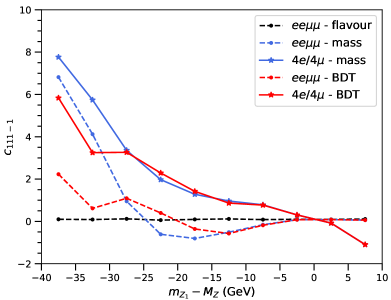
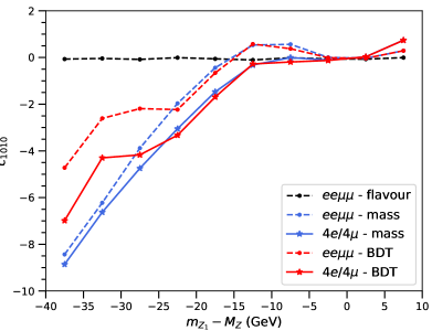
Figure 3: Dependence of the correlation coefficients $c_{111-1}$ and $c_{1010}$ on $m_{Z_{1}}$, using different methods to pair opposite-sign leptons.

Future prospects. We estimate the statistical sensitivity of these measurements at the high-luminosity upgrade of the LHC (HL-LHC), with a luminosity of 3 ab^-1. We consider $gg\to H\to ZZ\to 4\ell$ at 14 TeV, normalising the Higgs cross section to 54.67 pb and using branching ratios to $ee\mu\mu$ and $4e/4\mu$ of $5.9\times 10^{-5}$ and $6.5\times 10^{-5}$, respectively [11]. Hadronisation and parton showering are performed with Pythia [12] and detector simulation with Delphes [13] using the default card for the HL-LHC. Electrons are selected in the pseudorapidity region $|\eta|\leq 2.5$, and with transverse momentum $p_{T}\geq 7$ GeV. Muons are selected with $|\eta|\leq 2.7$ and $p_{T}\geq 5$ GeV. We require two opposite-sign same-flavour leptons. The three higher-$p_{T}$ leptons must satisfy minimum thresholds of 20, 15 and 10 GeV, respectively. These event selection requirements are quite close to those in Ref. [14]. In addition, we select a window $120\leq m_{4\ell}\leq 130$ GeV for the four-lepton invariant mass. In this region, the background has a size around 1/4 of the signal [14, 15]. The expected number of events in the $ee\mu\mu$, $4e$ and $4\mu$ final states are 1144, 379 and 1106, respectively. At the reconstructed level, $c_{111-1}$ and $c_{1010}$ exhibit moderate deviations from the parton-level values. We collect them in Table 1. For completeness we also give the values for the electroweak four-lepton background, calculated at the tree level, in the mass window $120\leq m_{4\ell}\leq 130$ GeV.

		Both pairings		Mass pairing
		$ee\mu\mu$	$4e/4\mu$	$ee\mu\mu$	$4e/4\mu$
$c_{111-1}$	($H$)	-0.76	-0.03	0.05	0.92
$c_{1010}$	($H$)	6.73	5.77	-0.30	-0.86
$c_{111-1}$	(bkg)	1.45	1.42	0.42	0.42
$c_{1010}$	(bkg)	7.67	7.68	-0.53	-0.69

‘

Table 1: Correlation coefficients $c_{111-1}$, $c_{1010}$ at the reconstructed level, for the $H\to ZZ$ signal (‘$H$’) and the electroweak background (‘bkg’).

The statistical uncertainty on $c_{111-1}$ and $c_{1010}$ is estimated by performing pseudo-experiments for each final state. In each pseudo-experiment, a subset of $N$ random events (the expected number of events for the final state considered) is drawn from the total sample, and for this subset the coefficients are determined from the distribution, without correction from detector-level to parton-level. A large number of $10^{5}$ pseudo-experiments is performed in order to obtain the probability density function (p.d.f.) of these quantities, and from it the statistical uncertainty. For the calculation of $c_{111-1}$, $c_{1010}$ we also apply an upper cut $m_{Z_{1}}\leq M_{Z}$. As it can be seen from Figs 1 and 3, the region $m_{Z_{1}}\sim M_{Z}$ provides little discrimination, and in some cases there is a sign flip in the coefficients for $m_{Z_{1}}\geq M_{Z}$. No further sensitivity optimisation is attempted. Results are presented in Table 2. The statistical significance ($Z$-score) of the differences are given in the last column. The first value corresponds to the comparison of $ee\mu\mu$ and $4e/4\mu$ channels (summing both flavours) and the second one to the comparison between $ee\mu\mu$ and $4\mu$.

	$ee\mu\mu$	$4e/4\mu$	$4\mu$	$Z$
$c_{111-1}$	$-0.88\pm 0.22$	$-0.03\pm 0.19$	$-0.06\pm 0.21$	2.9 | 2.7
$c_{1010}$	$7.68\pm 0.27$	$6.45\pm 0.23$	$6.47\pm 0.27$	3.5 | 3.2
$c_{111-1}$	$0.07\pm 0.35$	$1.20\pm 0.30$	$1.17\pm 0.35$	2.4 | 2.2
$c_{1010}$	$-0.43\pm 0.34$	$-1.13\pm 0.29$	$-1.14\pm 0.34$	1.6 | 1.5

Table 2: Central values and expected uncertainties for $c_{111-1}$ and $c_{1010}$ obtained from pseudo-experiments, in the different final states, and statistical significance of the differences (last column). The upper set of values is obtained with both pairings, and the lower one with mass pairing.

Quantum interference is probed by comparing the results obtained for the $ee\mu\mu$ and $4e/4\mu$ samples using both pairings (upper block of Table 2). The statistical differences for $c_{111-1}$ and $c_{1010}$ amount to $2.9\sigma$ and $3.5\sigma$, respectively. Their statistical correlation is -0.14, therefore both can easily be combined to obtain a significance of $4.9\sigma$. (Without the upper cut on $m_{Z_{1}}$, the statistical differences are of $2.6\sigma$ and $2.9\sigma$, and the combination amounts to $4.2\sigma$.) Identical-particle effects can be tested either using both pairings or mass pairing. The former gives more sensitive results. The comparison of $c_{111-1}$, $c_{1010}$ between $ee\mu\mu$ and $4\mu$ samples yields $2.7\sigma$ and $3.2\sigma$ which, when combined, provide an overall significance of $4.5\sigma$.

Further tests of identical-particle effects can be performed by comparing the full $m_{Z_{1}}$ distributions for $ee\mu\mu$ and $4e/4\mu$ final states (or $4\mu$ alone) obtained with mass pairing. The $p$-value giving the probability that two distributions result from the same p.d.f. is obtained using a Kolmogorov-Smirnov test [16, 17]. We perform $10^{5}$ pseudo-experiments, and for each one we calculate the $p$-value, which is then translated into a $Z$-score corresponding to the number of standard deviations. The mean value of the $Z$-score obtained over pseudo-experiments is the expected significance. For the difference between $ee\mu\mu$ and $4e/4\mu$ ($4\mu$) samples it amounts to $3.6\sigma$ ($3.2\sigma$). The distribution of $m_{Z_{2}}$ has a discriminating power below the $2\sigma$ level.

A final comment on the electroweak four-lepton background is in order. In the region of interest it is quite small, as mentioned; the coefficients are also quite similar in $ee\mu\mu$ and $4e/4\mu$ final states, as seen in Table 1. And they are of similar magnitude as the ones for $H\to ZZ$. Therefore, a background subtraction, which is out of the scope of the present work, seems feasible, and will only result in a mild increase of the statistical uncertainty in $c_{111-1}$ and $c_{1010}$, and a corresponding decrease of the significance with respect to the results presented here. Next-to-leading order corrections for the $ee\mu\mu$ final state are known [18], and provide a small shift in $c_{111-1}$ and $c_{1010}$ which is well below the statistical uncertainty.

Discussion. In this Letter we have proposed a novel probe of quantum interference in Higgs decays $H\to ZZ\to 4\ell$, based on angular correlations of the decay products. This test only relies on a data comparison between $ee\mu\mu$ and $4e/4\mu$ final states. This is in contrast to other proposals; for example, the ALICE Collaboration has measured an angular oscillating pattern in Pb-Pb collisions [19] that can be interpreted as quantum interference but only after compared to Monte Carlo predictions. Whereas, in Higgs decays one can even measure the analogous to ‘covering a slit’ to subsequently establish the presence of quantum interference by using data alone.

The measurements in Higgs decays can also be used to test identical-particle effects. To our knowledge, these would be the first tests to establish the identical-particle behaviour for muons. We have explored several observables that differ between $ee\mu\mu$ and $4e/4\mu$ final states, to conclude that the angular correlations used to probe quantum interference are also the most sensitive to establish the identical-particle behaviour. We have not considered the total decay width, whose difference between $ee\mu\mu$ and $4e/4\mu$ final states does not have a clear interpretation as due to identical-particle behaviour.

In our work we have focused, for simplicity, on the angular correlation coefficients $c_{111-1}$ and $c_{1010}$. Other terms in the distribution (1) exhibit differences between $ee\mu\mu$ and $4e/4\mu$ final states, and they could also be incorporated in an experimental analysis to improve the statistical significance of the discrimination. For example, $a_{20}^{1,2}$ show differences at the $1\sigma-2\sigma$ level, while the differences in $c_{222-2}$, $c_{212-1}$ and $c_{2020}$ are below $1\sigma$.

Electroweak $ZZ$ production with both $Z$ bosons on their mass shell has a larger cross section than $H\to ZZ$, but is not useful to probe interference and identical-particle effects. The correlation coefficients are very similar in $ee\mu\mu$ and $4e/4\mu$ final states, with differences at the few percent level. This is due to the small contribution of the interference between diagrams related by identical-particle exchange in the latter. Below the $ZZ$ threshold, four-lepton production can be mediated by virtual $Z$ and $\gamma$ exchange; however, the differences between $ee\mu\mu$ and $4e/4\mu$ final states are small — see for example Table 1 for the kinematical region near the Higgs peak. Then, $H\to ZZ\to 4\ell$, despite its small cross section, seems to be the most suited process to probe quantum interference and identical-particle effects, with an expected sensitivity at the $4\sigma$ level at the HL-LHC.

References

- [1] G. Aad et al. [ATLAS], “Observation of quantum entanglement with top quarks at the ATLAS detector,” Nature 633 (2024) no.8030, 542-547 [arXiv:2311.07288 [hep-ex]]. Briefing in https://atlas.cern/Updates/Briefing/TopEntanglement
- [2] A. Hayrapetyan et al. [CMS], “Observation of quantum entanglement in top quark pair production in proton–proton collisions at TeV,” Rept. Prog. Phys. 87 (2024) no.11, 117801 [arXiv:2406.03976 [hep-ex]]. Briefing in https://cms.cern/news/entangled-titansunravelingmysteries-quantummechanics-top-quarks
- [3] A. Hayrapetyan et al. [CMS], “Measurements of polarization and spin correlation and observation of entanglement in top quark pairs using lepton+jets events from proton-proton collisions at = 13 TeV,” [arXiv:2409.11067 [hep-ex]]. Briefing in https://cms.cern/news/spooky-action-distancebetween-heaviest-particles
- [4] C. K. Hong, Z. Y. Ou and L. Mandel, “Measurement of subpicosecond time intervals between two photons by interference,” Phys. Rev. Lett. 59 (1987), 2044-2046
- [5] A. Ashkin, L. A. Page and W. M. Woodward, “Electron-Electron and Positron-Electron Scattering Measurements” Phys. Rev. 94 (1954), 357–362
- [6] W. Bernreuther, D. Heisler and Z. G. Si, “A set of top quark spin correlation and polarization observables for the LHC: Standard Model predictions and new physics contributions,” JHEP 12 (2015), 026 [arXiv:1508.05271 [hep-ph]].
- [7] J. A. Aguilar-Saavedra, A. Bernal, J. A. Casas and J. M. Moreno, “Testing entanglement and Bell inequalities in ,” Phys. Rev. D 107 (2023) no.1, 016012 [arXiv:2209.13441 [hep-ph]].
- [8] J. A. Aguilar-Saavedra, J. Bernabéu, V. A. Mitsou and A. Segarra, “The boson spin observables as messengers of new physics,” Eur. Phys. J. C 77 (2017) no.4, 234 [arXiv:1701.03115 [hep-ph]].
- [9] T. Chen and C. Guestrin, “XGBoost: A Scalable Tree Boosting System´´ Proceedings of the 22nd ACM SIGKDD International Conference on Knowledge Discovery and Data Mining (KDD’16), 785 (2016) [arXiv:1603.02754 [hep-ph]].
- [10] J. Alwall, R. Frederix, S. Frixione, V. Hirschi, F. Maltoni, O. Mattelaer, H. S. Shao, T. Stelzer, P. Torrielli and M. Zaro, “The automated computation of tree-level and next-to-leading order differential cross sections, and their matching to parton shower simulations,” JHEP 07 (2014), 079 [arXiv:1405.0301 [hep-ph]].
- [11] M. Cepeda, S. Gori, P. Ilten, M. Kado, F. Riva, R. Abdul Khalek, A. Aboubrahim, J. Alimena, S. Alioli and A. Alves, et al. “Report from Working Group 2: Higgs Physics at the HL-LHC and HE-LHC,” CERN Yellow Rep. Monogr. 7 (2019), 221-584 [arXiv:1902.00134 [hep-ph]].
- [12] T. Sjostrand, S. Mrenna and P. Z. Skands, “A Brief Introduction to PYTHIA 8.1,” Comput. Phys. Commun. 178 (2008), 852-867 [arXiv:0710.3820 [hep-ph]].
- [13] J. de Favereau et al. [DELPHES 3], “DELPHES 3, A modular framework for fast simulation of a generic collider experiment,” JHEP 02 (2014), 057 [arXiv:1307.6346 [hep-ex]].
- [14] G. Aad et al. [ATLAS], “Test of CP-invariance of the Higgs boson in vector-boson fusion production and in its decay into four leptons,” JHEP 05 (2024), 105 [arXiv:2304.09612 [hep-ex]].
- [15] A. M. Sirunyan et al. [CMS], “Measurements of production cross sections of the Higgs boson in the four-lepton final state in proton–proton collisions at ,” Eur. Phys. J. C 81 (2021) no.6, 488 [arXiv:2103.04956 [hep-ex]].
- [16] A. N. Kolmogorov, “Sulla determinazione empirica di una legge di distribuzione,” Giornale dell’Istituto Italiano degli Attuari, 4, 83-91 (1933).
- [17] N. V. Smirnov, ”Table for Estimating the Goodness of Fit of Empirical Distributions,” The Annals of Mathematical Statistics, 19(2), 279-281 (1948)
- [18] M. Grossi, G. Pelliccioli and A. Vicini, “From angular coefficients to quantum observables: a phenomenological appraisal in di-boson systems,” [arXiv:2409.16731 [hep-ph]].
- [19] S. Acharya et al. [ALICE], “Measurement of the impact-parameter dependent azimuthal anisotropy in coherent photoproduction in Pb–Pb collisions at TeV,” Phys. Lett. B 858 (2024), 139017 [arXiv:2405.14525 [nucl-ex]]. Briefing in https://home.cern/news/news/physics/alice-doesdouble-slit