The two-loop fully differential soft function for $Q\bar{Q}V$ production at lepton colliders

Abstract

We consider the production of a pair of heavy quarks $Q\bar{Q}$ in association with a generic colour singlet system $V$ at lepton colliders, and present the first analytic calculation of the two-loop soft function differential in the total momentum of the real radiation. The calculation is performed by reducing the relevant Feynman integrals into a canonical basis of master integrals by means of integration-by-parts identities. The resulting integrals are then evaluated by solving a system of differential equations in the kinematic invariants, whose boundary conditions are determined analytically with some care due to the presence of Coulomb singularities. The fully differential soft function is expressed in terms of Goncharov polylogarithms. This result is an essential ingredient for a range of N³LL resummations for key collider observables at lepton colliders, such as the $Q\bar{Q}V$ production cross section at threshold and observables sensitive to the total transverse momentum of the radiation in heavy-quark final states. Moreover, it constitutes the complete final-final dipole contribution to the fully differential soft function needed for the description of $Q\bar{Q}V$ production at hadron colliders, which plays an important role in the LHC physics programme.

1 Introduction

The production of heavy quark pairs ($Q\bar{Q}$), optionally accompanied by a colour singlet system $V$, constitutes a key process at high-energy particle colliders. Both at future lepton colliders and at modern hadron colliders such as the LHC, this class of processes is relevant in the context of the precise extraction of properties of top and bottom quarks and of their couplings with the Higgs and electroweak gauge bosons (see e.g. Janot:2015mqv ; Janot:2015yza ; Vos:2016til ; CMS:2021klw ; CMS:2022tkv ; ATLAS:2023eld ; CMS:2024fdo ; ATLAS:2024gth ; CMS:2024mke ; ATLAS:2024moy ).

The theoretical description of physical observables measured on this final state is often plagued by the presence of large logarithmic corrections of infrared origin, that requires a resummation of the perturbative expansion at all orders. A class of important collider observables admits a factorisation theorem encoding the description of the infrared limit of the observable $v$ at leading power. Key examples of such factorisation theorems at lepton colliders are those describing the production cross section of the $Q\bar{Q}(V)$ system at threshold vonManteuffel:2014mva ; Gao:2014nva ; Gao:2014eea , the back-to-back limit of the energy-energy correlation PhysRevD.19.2018 ; PhysRevLett.41.1585 for heavy-quark final states and, in the case of hadronic collisions, the total transverse momentum of the final-state system with respect to the beam axis Zhu:2012ts ; Li:2013mia ; Catani:2014qha ; Catani:2018mei ; Ju:2024xhd . From a phenomenological viewpoint, such factorisation theorems for this class of processes can be used in the context of slicing methods for higher-order calculations Gao:2014nva ; Gao:2014eea ; Catani:2019iny ; Catani:2022mfv ; Buonocore:2022pqq as well as in the matching of next-to-next-to-leading order calculations to parton showers Mazzitelli:2020jio ; Mazzitelli:2021mmm ; Mazzitelli:2024ura .

An essential ingredient common to all the above factorisation theorems is the soft function, which describes the effect of soft radiation emitted from the eikonalised propagators of the energetic heavy quarks, as encoded in time-like (massive) Wilson lines. Interestingly, the soft functions relevant for a broad class of observables, such as the threshold and transverse momentum dependent (TMD) soft function, can be derived starting from a more exclusive soft function differential in the total momentum of the real radiation Li:2016axz ; Li:2016ctv . The fully differential soft function with two light-like Wilson lines has been calculated to three loops Li:2016ctv , while the corresponding result with time-like Wilson lines is unknown beyond the one-loop order. In this article we present the first two-loop calculation of the latter fully differential soft function in the context of the production of a $Q\bar{Q}V$ final state at lepton colliders. This calculation constitutes a key ingredient to improve the description of heavy-quark processes at future lepton colliders, and a consistent building block, that of final-final massive dipoles, for the corresponding calculation for $Q\bar{Q}V$ production at hadron colliders. In the hadron-collider case, the two-loop computation of the threshold soft function for $Q\bar{Q}$ production has been carried out in Refs. Czakon:2013hxa ; Wang:2018vgu , while numerical calculations have been performed for the corresponding TMD soft function averaged over the azimuthal angle of the final-state system in Refs. Angeles-Martinez:2018mqh ; Catani:2023tby . The analytic calculation of the fully differential soft function for $Q\bar{Q}V$ production at hadron colliders would be highly desirable. The information encoded in this object would allow for theoretical investigations on the structure of multi-leg soft functions with both light-like and time-like Wilson lines and, from a phenomenological viewpoint, it would be relevant for precision phenomenology involving heavy-quark final states, for instance in the context of higher-order calculations of azimuthal asymmetries Catani:2017tuc which are known to diverge in fixed-order perturbation theory.

The article is structured as follows. In Section 2 we introduce our notation and conventions, while Section 3 outlines the computational method adopted in our calculation up to two loops together with consistency checks. In Section 4 we perform the renormalisation and present our results. Finally, Section 5 contains our conclusions and outlook to future work. The arXiv submission of this article is accompanied by the analytic results for the fully differential soft function distributed as ancillary files.

2 Definition of the fully differential soft function

Let us consider the following process in lepton-lepton annihilation

$$l^{+}(\ell_{1})+l^{-}(\ell_{2})\to Q_{1}(q_{1})+\bar{Q}_{2}(q_{2})+V(q_{V})+X(q_{X})\,,$$ (1)

where $Q_{1,2}$ are heavy quarks with the same or distinct masses $q_{1,2}^{2}$, $V$ is a color singlet of momentum $q_{V}^{\mu}$, and $X$ denotes the additional QCD radiation of total momentum $q_{X}^{\mu}$. Here and below, we use $Q$ and $\varepsilon$ to denote the total energy of the collision and a low scale characterising soft emissions, respectively. At leading power in $\varepsilon/Q$, the cross section can be factorised in the framework of Soft Collinear Effective Theory (SCET) Bauer:2000yr ; Bauer:2001yt ; Bauer:2002nz ; Beneke:2002ph ; Beneke:2002ni as follows

$$\frac{d\sigma}{d^{4}q\,d\Omega}=\frac{1}{(2\pi)^{4}}\int d^{4}x\ e^{-i(q-q_{1}-q_{2}-q_{V})\cdot x}\ {\cal H}(\{q_{1},q_{2},q_{V}\})\ {\cal S}(x,\{v_{1},v_{2}\})\ +\ {\cal O}(\varepsilon/Q)\,,$$ (2)

where $d\Omega$ indicates the differential phase space element of the $Q_{1}Q_{2}X$ final state. The hard function ${\cal H}(\{q_{1},q_{2},q_{V}\})$ is the squared of the hard Wilson coefficient (see e.g. Ref. Gao:2014nva ), and $\cal S$ is the soft function defined as

$${\cal S}(x,\{v_{1},v_{2}\})=\frac{1}{N_{c}}{\rm tr}\left\langle 0\left|\overline{\bf T}\left[Y_{v_{1}}(x)Y_{v_{2}}^{\dagger}(x)\right]{\bf T}\left[Y_{v_{1}}^{\dagger}(0)Y_{v_{2}}(0)\right]\right|0\right\rangle\,,$$ (3)

where the trace is over color indices, and $Y_{v_{i}}$ is a soft Wilson line along the velocity $v_{i}$ of the $i$-th heavy quark

$$Y_{v_{i}}(x)={\bf P}\exp\left(-ig_{s}\int_{0}^{\infty}dt\ v_{i}\cdot A_{s}^{a}(x+tv_{i})\ {\bm{T}}^{a}\right)\,.$$ (4)

The cross section given in Eq. (2) is fully differential on the final-state kinematics, including on the total momentum of the real radiation. At leading power, the hard Wilson coefficient is not sensitive to the kinematics of soft emissions in the final state due to the decoupling of hard and soft interactions in the SCET Lagrangian, so $\cal H$ can be taken out from the Fourier transform. Since the cross section in Eq. (2) is fully exclusive in the radiation’s momentum, it can describe observables in various kinematic limits. We present two specific examples below.

The first is the production cross section for $Q_{1}Q_{2}V$ in the threshold limit, where the total energy of the soft QCD radiations $(q-q_{1}-q_{2}-q_{V})^{0}$ is constrained by $E_{\rm cut}\sim\varepsilon\ll Q$. The corresponding threshold soft function can be applied to study the next-to-next-to-leading order (NNLO) QCD corrections to heavy quark pair production in $e^{+}e^{-}$ annihilation with a phase-space slicing method vonManteuffel:2014mva ; Gao:2014nva ; Gao:2014eea . In this case, the spatial coordinate is fixed by $\delta^{3}(\vec{x})$ after integrating over $d^{3}\vec{q}$, so in the threshold limit Eq. (2) can be rewritten as

$$\frac{d\sigma(E_{\rm cut})}{d\Omega}={\cal H}(\{q_{1},q_{2},q_{V}\})\int_{0}^{E_{\rm cut}}dE\int\frac{dx^{0}}{2\pi}\ e^{-iE\,x^{0}}{\cal S}\left((x^{0},\vec{x}=0),\{v_{1},v_{2}\}\right)\ +\ {\cal O}(E_{\rm cut}/Q)\,.$$ (5)

A second example is that of global observables sensitive to the total transverse momentum of the radiation taken with respect to a reference axis. Observables in this class include the energy-energy-correlation PhysRevD.19.2018 ; PhysRevLett.41.1585 for massive quarks, or the transverse momentum of the $Q\bar{Q}V$ system w.r.t. the beam axis. The latter is in direct correspondence with the analogous observable in hadron collisions, of which the calculation presented in this article constitutes a self-consistent building block. Due to the absence of collinear singularities in the problem under consideration, the specific choice of the reference axis does not lead to additional logarithmic corrections (at leading power in $\varepsilon/Q$). We can therefore parametrise a generic momentum $p^{\mu}$ using the standard light-cone decomposition

$$p^{\mu}=(n\cdot p)\frac{{\bar{n}}^{\mu}}{2}+({\bar{n}}\cdot p)\frac{{n}^{\mu}}{2}+p_{\perp}^{\mu}\equiv p_{+}^{\mu}+p_{-}^{\mu}+p_{\perp}^{\mu}\,,$$ (6)

where $n$ and $\bar{n}$ are light-like vectors aligned to the reference directions (e.g. the beam), the total momentum of QCD emissions scales as

$$q_{X}^{\mu}=(q-q_{1}-q_{2}-q_{V})^{\mu}\sim Q(1,1,\varepsilon)\,,\qquad\mbox{with}\quad\varepsilon=q_{X,T}/Q\,,$$ (7)

with $q_{X,T}\equiv\sqrt{-q_{X,\perp}^{2}}$. The conjugate position-space coordinate $x^{\mu}$ then scales as $x^{\mu}\sim\left(Q\right)^{-1}(1,1,\varepsilon^{-1})$ where, by performing the multiple-pole expansion for the soft fields, the dependence on light-cone components $x_{+}$ and $x_{-}$ are suppressed compared to the perpendicular component $x_{\perp}$. Therefore, the cross section in Eq. (2) can be rewritten as

$$\frac{d\sigma}{d\Omega}=\frac{d^{2}q_{X,\perp}}{(2\pi)^{2}}\ {\cal H}(\{q_{1},q_{2},q_{V}\})\int d^{2}x_{\perp}\ e^{-iq_{X,\perp}\cdot x_{\perp}}\ {\cal S}(x_{\perp},\{v_{1},v_{2}\})\ +\ {\cal O}(q_{X,T}/Q)\,.$$ (8)

As shown in the above examples, the fully differential soft function with the full dependence on $x^{\mu}$ encodes information that is relevant in a range of factorisation theorems upon appropriate projections.

3 Calculation of the two-loop fully differential soft function

In the present section we will outline the main aspects of the calculation. We first introduce the setup and computational strategy, and then discuss both the NLO and NNLO results.

3.1 Fully differential soft function in momentum space

Eq. (3) defines the soft function in position space. Due to the convenience of evaluation of Feynman integrals in momentum space, it makes sense to perform the calculation in momentum space first, and then Fourier-transform the result back to position space. The fully differential soft function in momentum space can be defined as

$$S(\omega,\{\eta,v_{1},v_{2}\})=\frac{1}{N_{c}}{\rm tr}\left\langle 0\left|\overline{\bf T}\left[Y_{v_{1}}(0)Y_{v_{2}}^{\dagger}(0)\right]\delta(\omega-\eta\cdot\hat{p})\ {\bf T}\left[Y_{v_{1}}^{\dagger}(0)Y_{v_{2}}(0)\right]\right|0\right\rangle\,,$$ (9)

where $\eta^{\mu}$ is a dimensionless vector aligned with $x^{\mu}$, and ${\hat{p}}^{\mu}$ is an operator picking up the total momentum of soft radiations in the final state. With a Fourier transform, $S(\omega,\{\eta,v_{1},v_{2}\})$ can be related to the soft function in position space

$${\cal S}(x,\{v_{1},v_{2}\})=\int d\omega\ e^{i\omega t}\ S(\omega,\{\eta,v_{1},v_{2}\})\,,$$ (10)

where $t$ relates $\eta^{\mu}$ to $x^{\mu}$ by $x^{\mu}=t\eta^{\mu}$. The explicit $\eta^{\mu}$ and $t$ for threshold and TMD soft functions can be chosen as

$$\eta^{\mu}=(1,0,0,0)\,,\qquad\quad t=x^{0}\,,\qquad\mbox{and}$$ (11)

$$\eta^{\mu}=(0,-i\cos\phi,-i\sin\phi,0)\,,\qquad t=i\,x_{T}\,,$$ (12)

respectively, where $\phi$ is the azimuthal angle between $p_{\perp}$ and $x_{\perp}$, and $x_{T}\equiv\sqrt{-x_{\perp}^{2}}$. We stress that the fully differential soft function considered here is free of rapidity divergences. In the more general case of a fully differential soft function containing also light-like Wilson lines, one should supplement the correspondence given in Eq. (12) with a rapidity regularisation procedure. Within the exponential regularisation scheme of Ref. Li:2016axz , this would simply amount to adding a real time component to the vector $\eta^{\mu}$ in Eq. (12).

Since the soft Wilson lines in Eq. (9) are invariant under rescaling $v_{1}^{\mu}\to\alpha_{1}v_{1}^{\mu}$ and $v_{2}^{\mu}\to\alpha_{2}v_{2}^{\mu}$, the soft function depends on $v_{1}^{\mu}$ and $v_{2}^{\mu}$ only through cross ratios like $(v_{1}\cdot v_{2})/(\sqrt{v_{1}^{2}}\sqrt{v_{2}^{2}})$. In our case, there are only three independent cross ratios involved in the soft function, which can be chosen as (with a little abuse of notation we denote by $x$ one of these cross ratios, this is not to be confused with the coordinate $x^{\mu}$ used as argument of the fully differential soft function)

$$x=\frac{v_{1}\cdot v_{2}}{\sqrt{v_{1}^{2}}\sqrt{v_{2}^{2}}}\,,\qquad y=\frac{v_{1}\cdot\eta}{\sqrt{v_{1}^{2}}\sqrt{\eta^{2}}}\,,\qquad z=\frac{v_{2}\cdot\eta}{\sqrt{v_{2}^{2}}\sqrt{\eta^{2}}}\,.$$ (13)

Therefore, by dimensional counting in dimensional regularisation, the bare soft function takes the following generic form at $n$ loops

$$S^{(n)}(\omega,\{\eta,v_{1},v_{2}\};\epsilon)=\omega^{-1-2n\epsilon}\left(\frac{\eta^{2}}{4}\right)^{n\epsilon}f_{n}(x,y,z;\epsilon)\,,$$ (14)

where $\epsilon=(4-d)/2$ denotes the dimensional regulator, and we use the notation $S(\omega,\{\eta,v_{1},v_{2}\};\epsilon)=\delta(\omega)+\sum_{n=1}\left(\frac{\alpha_{s}}{4\pi}\right)^{n}S^{(n)}(\omega,\{\eta,v_{1},v_{2}\};\epsilon)$.

3.2 NLO calculation

Since purely virtual corrections are expressed by scaleless integrals, the NLO correction to the soft function only receives contributions from single-real radiation, which can be expressed as

$$S^{(1)}(\omega;\epsilon)=C_{\epsilon}^{(1)}C_{F}\int d^{d}k\ \delta^{+}(k^{2})\ \delta(\omega-\eta\cdot k)\left[\frac{v_{1}^{2}}{(v_{1}\cdot k)^{2}}+\frac{v_{2}^{2}}{(v_{2}\cdot k)^{2}}-\frac{2v_{1}\cdot v_{2}}{(v_{1}\cdot k)(v_{2}\cdot k)}\right]\,,$$ (15)

where $C_{\epsilon}^{(1)}=2e^{\epsilon\gamma_{E}}\pi^{\epsilon-1}$. Here and below, we omit the arguments $\{\eta,v_{1},v_{2}\}$ in the soft function for simplicity. Because of the complexity of the kinematics, it is still challenging to evaluate the one-loop phase space integrals directly. To accomplish analytical computation, we employ integration by parts (IBP) reduction Tkachov:1981wb ; Chetyrkin:1981qh and the method of differential equation (DE) Kotikov:1990kg ; Kotikov:1991hm ; Kotikov:1991pm ; Bern:1992em ; Bern:1993kr ; Remiddi:1997ny ; Gehrmann:1999as . To perform IBP reduction for phase space integrals, we need to replace the $\delta$ functions with propagators by means of reverse unitary Anastasiou:2002yz ; Anastasiou:2003yy ; Anastasiou:2003ds

$$\delta(x)=\frac{1}{2\pi i}\left(\frac{1}{x-i0}-\frac{1}{x+i0}\right)\equiv\mbox{Disc}(x^{-1})\,.$$ (16)

Then we rewrite $S^{(1)}(\omega;\epsilon)$ as

$$S^{(1)}(\omega;\epsilon)=C_{F}\ \omega^{-1-2\epsilon}\left(\frac{\eta^{2}}{4}\right)^{\epsilon}\left[v_{1}^{2}\ I_{1,1,2,0}+v_{2}^{2}\ I_{1,1,0,2}-2(v_{1}\cdot v_{2})\ I_{1,1,1,1}\right]\,,$$ (17)

with

$$I_{a_{1},a_{2},a_{3},a_{4}}=\kappa_{1}(\{a_{i}\})\ C_{\epsilon}^{(1)}\int\!d^{d}k\ \mbox{Disc}\left[(k^{2})^{-a_{1}}\right]\mbox{Disc}\left[(\omega-\eta\cdot k)^{-a_{2}}\right]\frac{(-1)^{a_{3}+a_{4}}}{(v_{1}\cdot k)^{a_{3}}(v_{2}\cdot k)^{a_{4}}}\,,$$ (18)

where the normalisation factor

$$\kappa_{1}(\{a_{i}\})=\omega^{2a_{1}+a_{2}+a_{3}+a_{4}-d}\left(\frac{\eta^{2}}{4}\right)^{(d-2a_{1}-a_{3}-a_{4})/2}$$

eliminates the dependence on $\omega$ and $\eta^{2}$. The parametrisation of the phase-space integrals given in Eq. (18) allows one to use standard Feynman integrals technology for their evaluation. By using the package FIRE6 Smirnov:2019qkx for IBP reduction, $S^{(1)}(\omega;\epsilon)$ is expressed in terms of a set of master integrals (MIs). Their derivatives with respect to the cross ratios can be obtained with the package LiteRed Lee:2013mka . To solve for the MIs, we choose the following basis of MIs with uniform transcendental weight (UT)

$${\vec{\mathcal{I}}}=\{\,2(1-2\epsilon)\,I_{1,1,0,0}\,,\ \epsilon\sqrt{1-1/z^{2}}\,I_{1,1,0,1}\,,\ \epsilon\sqrt{1-1/y^{2}}\,I_{1,1,1,0}\,,\ \epsilon\sqrt{1-1/x^{2}}\,I_{1,1,1,1}\}\,,$$ (19)

which leads to a simple DE system with $\epsilon$-form Henn:2013pwa

$$\partial_{x}\vec{{\mathcal{I}}}= \epsilon\left(\begin{array}[]{cccc}0&0&0&0\\ 0&0&0&0\\ 0&0&0&0\\ \frac{2}{\sqrt{x^{2}-1}}&\frac{-4\sqrt{z^{2}-1}(z-xy)}{\sqrt{x^{2}-1}\left(x^{2}-2xyz+y^{2}+z^{2}-1\right)}&\frac{-4\sqrt{y^{2}-1}(y-xz)}{\sqrt{x^{2}-1}\left(x^{2}-2xyz+y^{2}+z^{2}-1\right)}&\frac{2\left(\left(x^{2}+1\right)yz-xy^{2}-xz^{2}\right)}{\left(x^{2}-1\right)\left(x^{2}-2xyz+y^{2}+z^{2}-1\right)}\\ \end{array}\right)\cdot\vec{{\mathcal{I}}}\,,$$ (24)

$$\partial_{y}\vec{{\mathcal{I}}}= \epsilon\left(\begin{array}[]{cccc}0&0&0&0\\ 0&0&0&0\\ -\frac{1}{\sqrt{y^{2}-1}}&0&\frac{2y}{y^{2}-1}&0\\ 0&-\frac{4\sqrt{x^{2}-1}\sqrt{z^{2}-1}}{x^{2}-2xyz+y^{2}+z^{2}-1}&\frac{4\sqrt{x^{2}-1}(yz-x)}{\sqrt{y^{2}-1}\left(x^{2}-2xyz+y^{2}+z^{2}-1\right)}&\frac{2(y-xz)}{x^{2}-2xyz+y^{2}+z^{2}-1}\\ \end{array}\right)\cdot\vec{{\mathcal{I}}}\,,$$ (29)

$$\partial_{z}\vec{{\mathcal{I}}}= \epsilon\left(\begin{array}[]{cccc}0&0&0&0\\ -\frac{1}{\sqrt{z^{2}-1}}&\frac{2z}{z^{2}-1}&0&0\\ 0&0&0&0\\ 0&\frac{4\sqrt{x^{2}-1}(yz-x)}{\sqrt{z^{2}-1}\left(x^{2}-2xyz+y^{2}+z^{2}-1\right)}&-\frac{4\sqrt{x^{2}-1}\sqrt{y^{2}-1}}{x^{2}-2xyz+y^{2}+z^{2}-1}&\frac{2(z-xy)}{x^{2}-2xyz+y^{2}+z^{2}-1}\\ \end{array}\right)\cdot\vec{{\mathcal{I}}}\,.$$ (34)

The boundary conditions for solving the DEs are determined by the values of MIs at the phase space point $\eta^{\mu}=v_{1}^{\mu}=v_{2}^{\mu}$. These are obtained by recasting the denominators that were processed with reverse unitarity (see e.g. Eq. (18)) as delta functions, and performing the corresponding phase space integrals. They are given by

$$\vec{{\mathcal{I}}}_{0}=\left\{\frac{2e^{\epsilon\gamma_{E}}\Gamma(1-\epsilon)}{\Gamma(1-2\epsilon)},0,0,0\right\}\,.$$ (35)

By rationalizing the square roots in Eq. (24) with the change of variables

$$r=\sqrt{x^{2}-1}-x+1\,,\qquad t=\sqrt{y^{2}-1}-y+1\,,\qquad u=\sqrt{z^{2}-1}-z+1\,,$$ (36)

and solving the DEs order by order in $\epsilon$, the MIs are expressed in terms of Goncharov polylogarithms (GPLs), which can be defined iteratively as

$$G(a_{1},\dots\,a_{n};x)=\int_{0}^{x}\frac{dt}{t-a_{1}}G(a_{2},\dots\,a_{n};x)\,,$$ (37)

with $G(;x)=1$ and $G(\vec{0}_{n};x)=1/n!\,\ln^{n}x$ . At NLO, the letters involved in the arguments of GPLs are $\{0,1,2,\lambda_{1},\lambda_{2},\lambda_{3},\lambda_{4}\}$, where $\lambda_{i=1,\dots,4}$ are the roots of the polynomial $\lambda^{4}+\lambda^{3}(4yz-4)+4\lambda^{2}\left(y^{2}-3yz+z^{2}+1\right)-8\lambda(y-z)^{2}+4(y-z)^{2}=0\,$, and take the values

$$\lambda_{1}= 1-\sqrt{\left(y^{2}-1\right)\left(z^{2}-1\right)}-\sqrt{2y^{2}z^{2}+2yz\sqrt{\left(y^{2}-1\right)\left(z^{2}-1\right)}-y^{2}-z^{2}}-yz\,,$$

$$\lambda_{2}= 1-\sqrt{\left(y^{2}-1\right)\left(z^{2}-1\right)}+\sqrt{2y^{2}z^{2}+2yz\sqrt{\left(y^{2}-1\right)\left(z^{2}-1\right)}-y^{2}-z^{2}}-yz\,,$$

$$\lambda_{3}= 1-\sqrt{\left(y^{2}-1\right)\left(z^{2}-1\right)}-\sqrt{2y^{2}z^{2}-2yz\sqrt{\left(y^{2}-1\right)\left(z^{2}-1\right)}-y^{2}-z^{2}}-yz\,,$$

$$\lambda_{4}= 1-\sqrt{\left(y^{2}-1\right)\left(z^{2}-1\right)}+\sqrt{2y^{2}z^{2}-2yz\sqrt{\left(y^{2}-1\right)\left(z^{2}-1\right)}-y^{2}-z^{2}}-yz\,.$$ (38)

The result of NLO bare soft function will be presented in Sec. 4.

3.3 NNLO calculation

There are two types of contributions to the soft function at NNLO. One is from double real emissions (RR), and the other is from a single real emission with a one-loop virtual correction (RV). In principle, the RV contribution can be obtained by evaluating one-loop phase space integrals for the one-loop massive soft current Bierenbaum:2011gg ; Czakon:2018iev . However, it is quite challenging to perform the phase space integration without IBP reduction and the method of DE due to the complexity arising from the measurement of the fully differential soft function. Hence, we follow the same strategy to calculate the RR and RV NNLO contributions as that used for the NLO calculation.

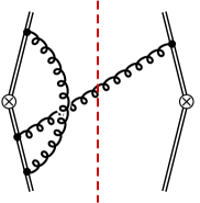
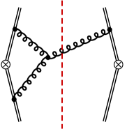
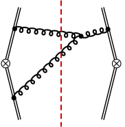
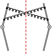
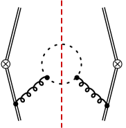
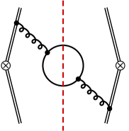
Figure 1: Examples for two-loop Feynman diagrams that contribute to the soft function $S(\omega;\epsilon)$.

To obtain the amplitudes, we generate the two-loop Feynman diagrams with qgraf  Nogueira:1991ex for both the RR and RV contributions individually. Some examples of two-loop graphs are shown in fig. 1. The Feynman gauge is employed for summing over gluon polarisation vectors, so the contribution of ghost fields to the vacuum polarisation diagrams has to be taken into account to cancel the contribution of unphysical gluon polarisations. After assigning the Feynman rules in momentum space and performing Dirac, Lorentz and color algebras, the amplitudes of the RR and RV contributions are expressed as linear combinations of scalar Feynman integrals with Cutkosky cuts. By means of partial-fraction decomposition for linear propagators followed by suitable shifts of the loop momentum, the scalar integrals can be mapped onto the integral topologies defined by complete bases of propagators, which fit to the setup of FIRE6.

For the RR contribution, the scalar integrals take the generic form

$$I^{{\rm RR}}_{\vec{a}}=\kappa_{2}(\{a_{i}\})\ C_{\epsilon}^{\rm RR}\int\!d^{d}k_{1}\int\!d^{d}k_{2}\, \mbox{Disc}\left[\left(k_{1}^{2}\right)^{-a_{1}}\right]\mbox{Disc}\left[\left(k_{2}^{2}\right)^{-a_{2}}\right]\mbox{Disc}\left[(\omega-\eta\cdot(k_{1}+k_{2}))^{-a_{3}}\right]$$

$$\times \frac{(-1)^{a_{4}+a_{5}+a_{6}+a_{7}+a_{8}}}{\left[(k_{1}+k_{2})^{2}\right]^{a_{4}}{\mathcal{D}}_{5}^{a_{5}}\,{\mathcal{D}}_{6}^{a_{6}}\,{\mathcal{D}}_{7}^{a_{7}}\,{\mathcal{D}}_{8}^{a_{8}}}\,,$$ (39)

where the normalisation factors read

$$\kappa_{2}(\{a_{i}\})=\omega^{2a_{1}+2a_{2}+a_{3}+2a_{4}+a_{5}+a_{6}+a_{7}+a_{8}-2d}\left(\frac{\eta^{2}}{4}\right)^{(2d-2a_{1}-2a_{2}-a_{3}-2a_{4}-a_{5}-a_{6}-a_{7}-a_{8})/2}\,,$$ (40)

and $C_{\epsilon}^{\rm RR}=-4\pi^{2\epsilon-2}$. As for the NLO case, the reverse unitarity representation of the phase-space integrals is used for the IBP reduction and to derive the canonical differential equations. The evaluation of the boundary conditions is then carried out by re-expressing the relevant denominators as delta functions. The denominators ${\mathcal{D}}_{5,6}$ and ${\mathcal{D}}_{7,8}$ correspond to propagators of Wilson lines along the $v_{1}$ and $v_{2}$ directions, respectively. After performing IBP reduction and remapping the MIs across the initial integral topologies with Kira Klappert:2020nbg , the RR amplitudes can be expressed by a linear combination of 31 MIs, which can be cast into the following five integral topologies defined by propagators $\{{\mathcal{D}}_{5},{\mathcal{D}}_{6},{\mathcal{D}}_{7},{\mathcal{D}}_{8}\}$ as

Topo RR1 : $$\qquad\left\{v_{1}\cdot k_{1}\,,v_{1}\cdot k_{2}\,,v_{2}\cdot k_{1}\,,v_{2}\cdot k_{2}\right\}\,,$$

Topo RR2 : $$\qquad\left\{v_{1}\cdot k_{1}\,,v_{1}\cdot\left(k_{1}+k_{2}\right)\,,v_{2}\cdot k_{1}\,,v_{2}\cdot k_{2}\right\}\,,$$

Topo RR3 : $$\qquad\left\{v_{1}\cdot k_{1}\,,v_{1}\cdot k_{2}\,,v_{2}\cdot k_{1}\,,v_{2}\cdot\left(k_{1}+k_{2}\right)\right\}\,,$$ (41)

Topo RR4 : $$\qquad\left\{v_{1}\cdot k_{1}\,,v_{1}\cdot\left(k_{1}+k_{2}\right)\,,v_{2}\cdot k_{1}\,,v_{2}\cdot\left(k_{1}+k_{2}\right)\right\}\,,$$

Topo RR5 : $$\qquad\left\{v_{1}\cdot k_{1}\,,v_{1}\cdot\left(k_{1}+k_{2}\right)\,,v_{2}\cdot k_{2}\,,v_{2}\cdot\left(k_{1}+k_{2}\right)\right\}\,.$$

For double-real integrals, the causal ‘$i0$’ prescriptions for the propagators can be neglected, because the denominators are always positive for on-shell momenta $k_{1,2}$. To build the DE system in $\epsilon$-form, we first find the candidate UT integrals by requiring that they have constant leading singularities Cachazo:2008vp ; Arkani-Hamed:2010pyv . The method of Magnus and Dyson series expansion Argeri:2014qva is also employed to convert the inhomogeneous terms of the DE into $\epsilon$-form. Eventually, the UT basis of the MIs reads

$$\vec{{\mathcal{I}}} {}^{\rm RR}=\Big{\{}\epsilon I_{2,2,1,0,0,0,0,0}^{{\rm RR}1}\,,~{}\frac{\epsilon^{2}\sqrt{z^{2}-1}}{z}I_{1,2,1,0,0,0,1,0}^{{\rm RR}1}\,,~{}\frac{\epsilon^{2}\sqrt{y^{2}-1}}{y}I_{1,2,1,0,1,0,0,0}^{{\rm RR}1}\,,~{}\frac{\epsilon^{2}\sqrt{y^{2}-1}}{y}I_{1,2,1,0,0,1,0,0}^{{\rm RR}2}\,,$$

$$\frac{\epsilon^{2}\sqrt{z^{2}-1}}{z}I_{1,2,1,0,0,0,0,1}^{{\rm RR}3}\,,~{}\frac{(1-4\epsilon)\epsilon^{2}\left(z^{2}-1\right)}{z^{2}}I_{1,1,1,0,0,0,1,1}^{{\rm RR}1}\,,~{}\frac{(1-4\epsilon)\epsilon^{2}\sqrt{y^{2}-1}\sqrt{z^{2}-1}}{yz}I_{1,1,1,0,0,1,1,0}^{{\rm RR}1}\,,$$

$$\frac{\epsilon^{2}\sqrt{x^{2}-1}}{x}I_{1,2,1,0,1,0,1,0}^{{\rm RR}1}\,,~{}\frac{(1-4\epsilon)\epsilon^{2}\left(y^{2}-1\right)}{y^{2}}I_{1,1,1,0,1,1,0,0}^{{\rm RR}1}\,,~{}\frac{\epsilon^{2}\sqrt{y^{2}-1}}{xz}I_{1,1,1,0,0,1,2,0}^{{\rm RR}2}\,,$$

$$\frac{\epsilon^{2}(4\epsilon-1)\left(x^{2}-2yzx+z^{2}\right)}{xyz}I_{1,1,1,0,0,1,1,0}^{{\rm RR}2}-\frac{\epsilon^{2}(xy-z)}{2x^{2}z}I_{1,1,1,0,0,1,2,0}^{{\rm RR}2}+\frac{\epsilon^{2}(xy-z)}{xy}I_{1,2,1,0,0,1,0,0}^{{\rm RR}2}\,,$$

$$\frac{(1-4\epsilon)\epsilon^{2}\left(y^{2}-1\right)}{y^{2}}I_{1,1,1,0,1,1,0,0}^{{\rm RR}2}\,,~{}\frac{\epsilon x}{\sqrt{x^{2}-1}}I_{2,2,1,0,0,0,0,0}^{{\rm RR}1}+\frac{8\epsilon^{2}(4\epsilon-1)\left(x^{2}-2yzx+z^{2}\right)}{yz\sqrt{x^{2}-1}}I_{1,1,1,0,0,1,1,0}^{{\rm RR}2}$$

$$\qquad+\frac{8\epsilon^{2}(z-xy)}{xz\sqrt{x^{2}-1}}I_{1,1,1,0,0,1,2,0}^{{\rm RR}2}+\frac{8\epsilon^{2}(xy-z)}{y\sqrt{x^{2}-1}}I_{1,2,1,0,0,1,0,0}^{{\rm RR}2}+\frac{\epsilon(2\epsilon+1)}{x\sqrt{x^{2}-1}}I_{1,2,1,0,0,1,0,1}^{{\rm RR}2}\,,$$

$$\frac{(1-4\epsilon)\epsilon^{2}\left(z^{2}-1\right)}{z^{2}}I_{1,1,1,0,0,0,1,1}^{{\rm RR}3}\,,~{}\frac{\epsilon^{2}\sqrt{z^{2}-1}}{xy}I_{1,1,1,0,2,0,0,1}^{{\rm RR}3}\,,$$

$$\frac{\epsilon^{2}(4\epsilon-1)\left(x^{2}-2yzx+y^{2}\right)}{xyz}I_{1,1,1,0,1,0,0,1}^{{\rm RR}3}+\frac{\epsilon^{2}(y-xz)}{2x^{2}y}I_{1,1,1,0,2,0,0,1}^{{\rm RR}3}+\frac{\epsilon^{2}(xz-y)}{xz}I_{1,2,1,0,0,0,0,1}^{{\rm RR}3}\,,$$

$$\frac{\epsilon x}{\sqrt{x^{2}-1}}I_{2,2,1,0,0,0,0,0}^{{\rm RR}1}+\frac{8\epsilon^{2}(4\epsilon-1)\left(x^{2}-2yzx+y^{2}\right)}{yz\sqrt{x^{2}-1}}I_{1,1,1,0,1,0,0,1}^{{\rm RR}3}+\frac{8\epsilon^{2}(y-xz)}{xy\sqrt{x^{2}-1}}I_{1,1,1,0,2,0,0,1}^{{\rm RR}3}$$

$$\qquad+\frac{8\epsilon^{2}(xz-y)}{z\sqrt{x^{2}-1}}I_{1,2,1,0,0,0,0,1}^{{\rm RR}3}+\frac{\epsilon(2\epsilon+1)}{x\sqrt{x^{2}-1}}I_{1,2,1,0,0,1,0,1}^{{\rm RR}3}\,,~{}\frac{\epsilon^{2}\sqrt{x^{2}-1}}{x}I_{1,2,1,0,0,1,0,1}^{{\rm RR}4}\,,$$

$$\frac{\epsilon^{3}\sqrt{x^{2}-1}\sqrt{z^{2}-1}}{xz}I_{1,1,1,0,1,0,1,1}^{{\rm RR}1}\,,~{}\frac{\epsilon^{3}\sqrt{x^{2}-1}\sqrt{y^{2}-1}}{xy}I_{1,1,1,0,1,1,1,0}^{{\rm RR}1}\,,~{}\frac{\epsilon^{3}\sqrt{x^{2}-1}\sqrt{y^{2}-1}}{xy}I_{1,1,1,0,1,1,0,1}^{{\rm RR}2}\,,$$

$$\frac{\epsilon^{3}\sqrt{x^{2}-1}\sqrt{y^{2}-1}}{xy}I_{1,1,1,0,1,1,1,0}^{{\rm RR}2}\,,~{}\frac{\epsilon^{3}\sqrt{x^{2}-1}}{x}I_{1,1,1,1,1,0,0,1}^{{\rm RR}2}\,,~{}\frac{\epsilon^{3}\sqrt{y^{2}-1}}{y}I_{1,1,1,1,1,0,-1,1}^{{\rm RR}2}\,,$$

$$\frac{\epsilon^{3}\sqrt{z^{2}-1}}{z}I_{1,1,1,1,1,-1,0,1}^{{\rm RR}2}\,,~{}4\epsilon^{2}I_{1,2,1,0,1,0,0,0}^{{\rm RR}1}+8\epsilon^{3}I_{1,1,1,1,1,0,-1,1}^{{\rm RR}2}+2\epsilon^{3}I_{1,1,1,1,1,0,0,1}^{{\rm RR}2}+\frac{\epsilon^{2}z}{xy}I_{1,1,1,1,2,0,-1,1}^{{\rm RR}2}\,,$$

$$\frac{\epsilon^{3}\sqrt{x^{2}-1}\sqrt{z^{2}-1}}{xz}I_{1,1,1,0,0,1,1,1}^{{\rm RR}3}\,,~{}\frac{\epsilon^{3}\sqrt{x^{2}-1}\sqrt{z^{2}-1}}{xz}I_{1,1,1,0,1,0,1,1}^{{\rm RR}3}\,,~{}\frac{\epsilon^{3}\left(x^{2}-1\right)}{x^{2}}I_{1,1,1,0,1,1,1,1}^{{\rm RR}1}\,,$$

$$\frac{\epsilon^{3}\left(x^{2}-1\right)}{x^{2}}I_{1,1,1,0,1,1,1,1}^{{\rm RR}4}\,,~{}\frac{\epsilon^{3}\left(x^{2}-1\right)}{x^{2}}I_{1,1,1,0,1,1,1,1}^{{\rm RR}5}\Big{\}}\,,$$ (42)

where the normalisation factors are obtained from the evaluation of the leading singularities of corresponding integrals in Baikov representation Baikov:1996rk ; Baikov:2005nv . The boundary conditions are determined at the point $v_{1}^{\mu}=v_{2}^{\mu}=\eta^{\mu}$. By using the Mellin-Barnes technique Smirnov:1999gc ; Tausk:1999vh implemented in the MB package Czakon:2005rk ; Smirnov:2009up , we obtain the analytical results for the boundary conditions as

$${\mathcal{I}}^{\rm RR}_{1,26}\Big{|}_{x=y=z=1} =8-\frac{28\pi^{2}\epsilon^{2}}{3}-\frac{496\zeta_{3}\epsilon^{3}}{3}-\frac{\pi^{4}\epsilon^{4}}{5}+{\mathcal{O}}(\epsilon^{5})\,,$$ (43)

$${\mathcal{I}}^{\rm RR}_{i}|_{x=y=z=1} =0\qquad\mbox{for}\quad i\neq 1~{}\mbox{and}~{}26\,.$$

After performing the rationalisation of the square roots shown in Eq. (36) and solving the DE equations order by order in $\epsilon$, the MIs can be expressed in terms of GPLs. The corresponding letters involved in the arguments of the GPLs are $\{0\,,1\,,2\,,1-y\,,(y-1)/y\,,\lambda_{i=1,\dots,18}\}$. $\lambda_{i=1,\dots,4}$ are the same as the letters in Eq. (3.2), while $\lambda_{i=5,\dots,8}$, $\lambda_{i=9,\dots,12}$, $\lambda_{i=13,\dots,16}$ and $\lambda_{i=17,18}$ are the roots of the polynomial equations

$$\lambda^{4}+\lambda^{3}(4yz-4)+4\lambda^{2}\left(z^{2}-3yz+2\right)-8\lambda\left(z^{2}-2yz+1\right)+4\left(z^{2}-2yz+1\right)=0\,,$$

$$\lambda^{4}+\lambda^{3}(4yz-4)+4\lambda^{2}\left(y^{2}-3yz+2\right)-8\lambda\left(y^{2}-2yz+1\right)+4\left(y^{2}-2yz+1\right)=0\,,$$

$$\lambda^{4}+4\lambda^{3}(y-1)-12\lambda^{2}(y-1)+16\lambda(y-1)-8(y-1)=0\,,$$

$$\lambda^{2}+2\lambda(y-1)-2(y-1)=0\,,$$ (44)

respectively.

The RV contribution is addressed with a similar procedure. The real-virtual integrals can be written as

$$I^{{\rm RV}}_{\vec{a}}=\kappa_{2}(\{a_{i}\})\ C_{\epsilon}^{\rm RV}\int \!d^{d}k_{1}\,\mbox{Disc}\left[\left(k_{1}^{2}\right)^{-a_{1}}\right]\mbox{Disc}\left[(\omega-\eta\cdot k_{1})^{-a_{3}}\right]$$

$$\times \int\!d^{d}k_{2}\,\frac{(-1)^{a_{2}+a_{4}+a_{5}+a_{6}+a_{7}+a_{8}}}{\left(k_{2}^{2}+i0\right)^{a_{2}}\left[(k_{1}+k_{2})^{2}+i0\right]^{a_{4}}{\mathcal{D}}_{5}^{a_{5}}\,{\mathcal{D}}_{6}^{a_{6}}\,{\mathcal{D}}_{7}^{a_{7}}\,{\mathcal{D}}_{8}^{a_{8}}}\,,$$ (45)

with $C_{\epsilon}^{\rm RV}=2i\pi^{2\epsilon-3}e^{2\gamma_{E}}$. After IBP reduction, the amplitudes can be expressed by a linear combination of 20 MIs, which can be remapped into three integral topologies defined by the propagators $\{{\mathcal{D}}_{5}\,,{\mathcal{D}}_{6}\,,{\mathcal{D}}_{7}\,,{\mathcal{D}}_{8}\}$ as

Topo RV1 : $$\qquad\left\{v_{1}\cdot k_{1}\,,-v_{1}\cdot k_{2}+i0\,,v_{2}\cdot k_{1}\,,-v_{2}\cdot k_{2}+i0\right\}\,,$$

Topo RV2 : $$\qquad\left\{v_{1}\cdot k_{1}\,,-v_{1}\cdot k_{2}+i0\,,v_{2}\cdot k_{2}+i0\,,v_{2}\cdot\left(k_{1}+k_{2}\right)+i0\right\}\,,$$

Topo RV3 : $$\qquad\left\{v_{1}\cdot k_{2}+i0\,,v_{1}\cdot\left(k_{1}+k_{2}\right)+i0\,,v_{2}\cdot k_{1}\,,-v_{2}\cdot k_{2}+i0\right\}\,.$$ (46)

Unlike for the RR case, here we have to indicate the causal ‘$i0$’ prescriptions explicitly for the propagators depending on the virtual momentum $k_{2}^{\mu}$, because they determine the sign of the imaginary part of the one-loop virtual correction. To build the DE system in $\epsilon$-form, we convert the set of MIs to the UT basis as follow

$$\vec{{\mathcal{I}}} {}^{\rm RV}=\Big{\{}\frac{\epsilon y}{xz}I_{2,0,1,1,0,0,0,2}^{{\rm RV}1}\,,\frac{\epsilon^{2}\sqrt{z^{2}-1}}{z}I_{1,0,1,2,0,0,0,1}^{{\rm RV}1}\,,\frac{\epsilon z}{xy}I_{2,0,1,1,0,2,0,0}^{{\rm RV}1}\,,\frac{\epsilon^{2}\sqrt{y^{2}-1}}{y}I_{1,0,1,2,0,1,0,0}^{{\rm RV}1}\,,$$

$$\frac{\epsilon^{2}\sqrt{z^{2}-1}}{xy}I_{1,0,1,1,0,2,1,0}^{{\rm RV}1}\,,\frac{\epsilon^{2}\sqrt{x^{2}-1}}{x}I_{1,0,1,2,0,1,1,0}^{{\rm RV}1}\,,\frac{\epsilon^{2}\sqrt{y^{2}-1}}{xz}I_{1,0,1,1,1,0,0,2}^{{\rm RV}1}\,,\frac{\epsilon^{2}\sqrt{x^{2}-1}}{x}I_{1,0,1,2,1,0,0,1}^{{\rm RV}1}\,,$$

$$\frac{\epsilon^{2}\sqrt{x^{2}-1}}{x}I_{2,0,1,1,0,1,0,1}^{{\rm RV}2}\,,\frac{\epsilon^{2}\sqrt{x^{2}-1}\sqrt{y^{2}-1}}{xy}I_{1,0,1,1,0,2,0,1}^{{\rm RV}2}\,,\frac{\epsilon^{2}\sqrt{x^{2}-1}}{x}I_{2,1,1,0,0,1,0,1}^{{\rm RV}2}\,,$$

$$\frac{\epsilon^{2}\sqrt{x^{2}-1}\sqrt{z^{2}-1}}{xz}I_{1,1,1,0,0,1,0,2}^{{\rm RV}2}\,,\frac{\epsilon^{3}\sqrt{x^{2}-1}\sqrt{y^{2}-1}}{xy}I_{1,1,1,0,1,1,0,1}^{{\rm RV}2}\,,\epsilon^{2}\left(1-1/x^{2}\right)I_{1,1,1,0,1,1,0,2}^{{\rm RV}2}\,,$$

$$\frac{\epsilon^{3}\sqrt{x^{2}-1}}{x}I_{1,1,1,1,0,1,0,1}^{{\rm RV}2}\,,\frac{\epsilon^{3}\sqrt{y^{2}-1}}{y}I_{1,1,1,1,0,1,-1,1}^{{\rm RV}2}-\frac{\epsilon^{3}\sqrt{y^{2}-1}}{y}I_{1,1,1,1,0,1,0,0}^{{\rm RV}2}\,,$$

$$\frac{\epsilon^{3}\sqrt{z^{2}-1}}{z}I_{1,1,1,1,-1,1,0,1}^{{\rm RV}2}-\frac{\epsilon^{3}\sqrt{z^{2}-1}}{z}I_{1,1,1,1,0,0,0,1}^{{\rm RV}2}\,,8\epsilon^{3}I_{1,1,1,1,-1,1,0,1}^{{\rm RV}2}-8\epsilon^{3}I_{1,1,1,1,0,0,0,1}^{{\rm RV}2}$$

$$\qquad+2\epsilon^{3}I_{1,1,1,1,0,1,0,1}^{{\rm RV}2}+\frac{\epsilon^{2}y}{xz}I_{1,1,1,1,-1,1,0,2}^{{\rm RV}2}-\frac{\epsilon^{2}y}{xz}I_{1,1,1,1,0,0,0,2}^{{\rm RV}2}-4\epsilon^{2}I_{1,0,1,2,0,0,0,1}^{{\rm RV}1}\,,$$

$$\frac{\epsilon^{3}\sqrt{x^{2}-1}\sqrt{z^{2}-1}}{xz}I_{1,1,1,0,0,1,1,1}^{{\rm RV}3}\,,\epsilon^{2}\left(1-1/x^{2}\right)I_{1,1,1,0,0,2,1,1}^{{\rm RV}3}\Big{\}}\,.$$ (47)

The boundary conditions are also determined at $v_{1}^{\mu}=v_{2}^{\mu}=\eta^{\mu}$. However, Coulomb singularities are encountered at this boundary point, because of the interaction between the two massive quarks at rest via the exchange of virtual gluons. Therefore, we have to resolve the singular behavior of the MIs in the limit of $x\to 1$ (i.e. $r\to 0$) before expanding them in $\epsilon$. As a result, we obtain the following analytical expressions for the boundary conditions

$${\mathcal{I}}^{\rm RV}_{1,3}\Big{|}_{x=y=z=1} =-8-16i\pi\epsilon+\frac{44\pi^{2}\epsilon^{2}}{3}+\left(\frac{112\zeta_{3}}{3}+8i\pi^{3}\right)\epsilon^{3}+\left(-\frac{127\pi^{4}}{45}+\frac{224i\pi}{3}\zeta_{3}\right)\epsilon^{4}+{\mathcal{O}}(\epsilon^{5})\,,$$

$${\mathcal{I}}^{\rm RV}_{9,11}\Big{|}_{x=y=z=1} =-16\,i\pi\,(2r)^{2\epsilon}\,e^{i\pi\epsilon}e^{2\epsilon\gamma_{E}}\,\epsilon^{2}\,\Gamma(2\epsilon)\,$$ (48)

$${\mathcal{I}}^{\rm RV}_{i}\Big{|}_{x=y=z=1} =0\qquad\mbox{for}~{}i\neq 1,3,9~{}\mbox{and}~{}11\,.$$

These boundary conditions have been cross checked with the results in ref. Bierenbaum:2011gg . Finally, by solving the DE equations order by order in $\epsilon$, the MIs can be expressed by GPLs with the same letters as for the NLO MIs. As a further test of the NNLO calculation, we calculate all RR and RV MIs using the package AMFlow Liu:2022chg with high numerical precision at random benchmark points, finding complete agreement with the analytic calculation.

4 Renormalisation and final result

With the calculation outlined in the previous sections, the two-loop bare soft function can be expressed as

$$S(\omega;\epsilon)= \delta(\omega)+\frac{Z_{\alpha}\alpha_{s}}{4\pi}\frac{1}{\omega}\left(\frac{\mu}{\hat{\omega}}\right)^{2\epsilon}C_{F}K_{F}(x,y,z)$$

$$+\left(\frac{Z_{\alpha}\alpha_{s}}{4\pi}\right)^{2}\frac{1}{\omega}\left(\frac{\mu}{\hat{\omega}}\right)^{4\epsilon}C_{F}\left[C_{F}K_{FF}(x,y,z)+C_{A}K_{FA}(x,y,z)+n_{f}T_{F}K_{Ff}(x,y,z)\right]\,,$$ (49)

where $\hat{\omega}=\omega/\sqrt{\eta^{2}/4}$, and $Z_{\alpha}\alpha_{s}\mu^{2\epsilon}$ gives the bare QCD coupling constant with

$$Z_{\alpha}=1+\frac{\alpha_{s}}{4\pi}\left(-\frac{\beta_{0}}{\epsilon}\right)+\left(\frac{\alpha_{s}}{4\pi}\right)^{2}\left(\frac{\beta_{0}^{2}}{\epsilon^{2}}-\frac{\beta_{1}}{2\epsilon}\right)+{\cal O}\left(\alpha_{s}^{3}\right)\,.$$ (50)

The NLO coefficient $K_{F}(x,y,z)$ is given by

$$K_{F}= -\frac{8x}{\sqrt{x^{2}-1}}G_{1,r}-8+8\epsilon\Bigg{(}\frac{y}{\sqrt{y^{2}-1}}G_{1,t}+\frac{z}{\sqrt{z^{2}-1}}G_{1,u}$$

$$\qquad-\frac{x}{\sqrt{x^{2}-1}}\Big{[}G_{\lambda_{1},1,r}+G_{\lambda_{2},1,r}+G_{\lambda_{3},1,r}+G_{\lambda_{4},1,r}-2G_{0,1,r}-2G_{2,1,r}$$

$$\qquad\quad+G_{1,t}\left(G_{\lambda_{1},r}-G_{\lambda_{2},r}-G_{\lambda_{3},r}+G_{\lambda_{4},r}\right)+G_{1,u}\left(G_{\lambda_{1},r}-G_{\lambda_{2},r}+G_{\lambda_{3},r}-G_{\lambda_{4},r}\right)\Big{]}\Bigg{)}$$

$$+2\epsilon^{2}\Bigg{(}\pi^{2}+\frac{8y}{\sqrt{y^{2}-1}}\left(G_{0,1,t}-G_{1,1,t}+G_{2,1,t}\right)+\frac{8z}{\sqrt{z^{2}-1}}\left(G_{0,1,u}-G_{1,1,u}+G_{2,1,u}\right)$$

$$\quad+\frac{x}{\sqrt{x^{2}-1}}\Big{[}\pi^{2}G_{1,r}-8\left(G_{\lambda_{1},r}-G_{\lambda_{2},r}-G_{\lambda_{3},r}+G_{\lambda_{4},r}\right)\left(G_{0,1,t}-G_{1,1,t}+G_{2,1,t}\right)$$

$$\qquad-8\left(G_{\lambda_{1},r}-G_{\lambda_{2},r}+G_{\lambda_{3},r}-G_{\lambda_{4},r}\right)\left(G_{0,1,u}-G_{1,1,u}+G_{2,1,u}\right)$$

$$\qquad+4G_{1,t}\Big{(}2G_{0,\lambda_{1},r}-2G_{0,\lambda_{2},r}-2G_{0,\lambda_{3},r}+2G_{0,\lambda_{4},r}+2G_{2,\lambda_{1},r}-2G_{2,\lambda_{2},r}$$

$$\qquad\quad-2G_{2,\lambda_{3},r}+2G_{2,\lambda_{4},r}-G_{\lambda_{1},\lambda_{1},r}+G_{\lambda_{1},\lambda_{2},r}+G_{\lambda_{1},\lambda_{3},r}-G_{\lambda_{1},\lambda_{4},r}$$

$$\qquad\quad-G_{\lambda_{2},\lambda_{1},r}+G_{\lambda_{2},\lambda_{2},r}+G_{\lambda_{2},\lambda_{3},r}-G_{\lambda_{2},\lambda_{4},r}-G_{\lambda_{3},\lambda_{1},r}+G_{\lambda_{3},\lambda_{2},r}$$

$$\qquad\quad+G_{\lambda_{3},\lambda_{3},r}-G_{\lambda_{3},\lambda_{4},r}-G_{\lambda_{4},\lambda_{1},r}+G_{\lambda_{4},\lambda_{2},r}+G_{\lambda_{4},\lambda_{3},r}-G_{\lambda_{4},\lambda_{4},r}\Big{)}$$

$$\qquad+4G_{1,u}\Big{(}2G_{0,\lambda_{1},r}-2G_{0,\lambda_{2},r}+2G_{0,\lambda_{3},r}-2G_{0,\lambda_{4},r}+2G_{2,\lambda_{1},r}-2G_{2,\lambda_{2},r}$$

$$\qquad\quad+2G_{2,\lambda_{3},r}-2G_{2,\lambda_{4},r}-G_{\lambda_{1},\lambda_{1},r}+G_{\lambda_{1},\lambda_{2},r}-G_{\lambda_{1},\lambda_{3},r}+G_{\lambda_{1},\lambda_{4},r}$$

$$\qquad\quad-G_{\lambda_{2},\lambda_{1},r}+G_{\lambda_{2},\lambda_{2},r}-G_{\lambda_{2},\lambda_{3},r}+G_{\lambda_{2},\lambda_{4},r}-G_{\lambda_{3},\lambda_{1},r}+G_{\lambda_{3},\lambda_{2},r}$$

$$\qquad\quad-G_{\lambda_{3},\lambda_{3},r}+G_{\lambda_{3},\lambda_{4},r}-G_{\lambda_{4},\lambda_{1},r}+G_{\lambda_{4},\lambda_{2},r}-G_{\lambda_{4},\lambda_{3},r}+G_{\lambda_{4},\lambda_{4},r}\Big{)}$$

$$\qquad-4\Big{(}4G_{0,0,1,r}+4G_{0,2,1,r}-2G_{0,\lambda_{1},1,r}-2G_{0,\lambda_{2},1,r}-2G_{0,\lambda_{3},1,r}-2G_{0,\lambda_{4},1,r}$$

$$\qquad\quad+4G_{2,0,1,r}+4G_{2,2,1,r}-2G_{2,\lambda_{1},1,r}-2G_{2,\lambda_{2},1,r}-2G_{2,\lambda_{3},1,r}-2G_{2,\lambda_{4},1,r}$$

$$\qquad\quad-2G_{\lambda_{1},0,1,r}-2G_{\lambda_{1},2,1,r}+G_{\lambda_{1},\lambda_{1},1,r}+G_{\lambda_{1},\lambda_{2},1,r}+G_{\lambda_{1},\lambda_{3},1,r}+G_{\lambda_{1},\lambda_{4},1,r}$$

$$\qquad\quad-2G_{\lambda_{2},0,1,r}-2G_{\lambda_{2},2,1,r}+G_{\lambda_{2},\lambda_{1},1,r}+G_{\lambda_{2},\lambda_{2},1,r}+G_{\lambda_{2},\lambda_{3},1,r}+G_{\lambda_{2},\lambda_{4},1,r}$$

$$\qquad\quad-2G_{\lambda_{3},0,1,r}-2G_{\lambda_{3},2,1,r}+G_{\lambda_{3},\lambda_{1},1,r}+G_{\lambda_{3},\lambda_{2},1,r}+G_{\lambda_{3},\lambda_{3},1,r}+G_{\lambda_{3},\lambda_{4},1,r}$$

$$\qquad\quad-2G_{\lambda_{4},0,1,r}-2G_{\lambda_{4},2,1,r}+G_{\lambda_{4},\lambda_{1},1,r}+G_{\lambda_{4},\lambda_{2},1,r}+G_{\lambda_{4},\lambda_{3},1,r}+G_{\lambda_{4},\lambda_{4},1,r}\Big{)}\Big{]}\Bigg{)}$$

$$+O\left(\epsilon^{3}\right)\,,$$ (51)

where we denoted $G_{a_{1},\dots,a_{n},x}=G(a_{1},\dots,a_{n};x)$ for brevity. The UV renormalisation of the soft function is more conveniently performed in Laplace space, because the Laplace transform

$$\tilde{S}(L;\epsilon)\equiv\int_{0}^{\infty}d\omega\,\exp\left(-\frac{\omega}{s\,e^{\gamma_{E}}}\right)S(\omega;\epsilon)\,,\qquad\mbox{with}\quad L=\ln\left(\frac{2s}{\mu\sqrt{\eta^{2}}}\right)\,,$$ (52)

turns the momentum-space convolutions between renormalisation factor and soft function into local products. One can show that, thanks to the correspondence of $S(\omega;\epsilon)$ with the threshold and TMD soft functions discussed in Sec. 3.1, the renormalisation of $\tilde{S}(L)$ is multiplicative (local). A simple way of seeing this is to boost the fully differential soft function into the rest frame of the $\eta^{\mu}$ vector, hence highlighting the direct correspondence with the threshold soft function, whose renormalisation is multiplicative in Laplace space.

The Laplace transform of the bare soft function in Eq. (4) can be achieved straightforwardly by the replacement

$$\frac{1}{\omega}\left(\frac{\mu}{\hat{\omega}}\right)^{n\epsilon}\to e^{-n\epsilon(L+\gamma_{E})}\Gamma(-n\epsilon)\,.$$ (53)

The ultraviolet (UV) poles in the bare soft function can be absorbed into the renormalisation factor defined in the $\overline{\rm MS}$ scheme

$$\tilde{S}(L;\epsilon)=Z_{S}(\epsilon,\mu)\,\tilde{S}(L,\mu)\,.$$ (54)

The RG equation of the soft function is given by

$$\frac{d}{d\ln\mu}\tilde{S}(L,\mu)=\Gamma^{S}(\alpha_{s})\,\tilde{S}(L,\mu)\,.$$ (55)

The RG equation of the hard function in Eq. (2) takes the same form for RG consistency.

4.1 Anomalous dimension of the fully differential soft function

Since the cross section is free of singularities, the UV poles of the bare soft function have to cancel against the infrared (IR) poles of the hard function ${\cal H}(\{q_{1},q_{2},q_{V}\};\epsilon)$, which are governed by the anomalous dimension Korchemsky:1987wg ; Korchemsky:1991zp ; Kidonakis:2009ev ; Becher:2009kw

$$\Gamma_{QQ}(\{v_{1},v_{2}\},\alpha_{s})=C_{F}\gamma_{\rm cusp}(\beta,\alpha_{s})+2\gamma^{Q}(\alpha_{s})\,,$$ (56)

where $\gamma_{\rm cusp}(\beta,\alpha_{s})$ is the massive cusp anomalous dimension

$$\gamma_{\rm{cusp}}(\beta,\alpha_{s})= \gamma_{\rm{cusp}}(\alpha_{s})\beta\coth\beta$$

$$+\frac{C_{A}}{2}\left(\frac{\alpha_{s}}{\pi}\right)^{2}\Bigg{[}\left(\text{Li}_{3}\left(e^{-2\beta}\right)+\beta\text{Li}_{2}\left(e^{-2\beta}\right)+\frac{\beta^{3}}{3}+\frac{\pi^{2}}{6}\beta-\zeta_{3}\right)\coth^{2}\beta$$

$$\qquad+\left(\text{Li}_{2}\left(e^{-2\beta}\right)-2\beta\ln\left(1-e^{-2\beta}\right)-\frac{\pi^{2}}{6}(\beta+1)-\beta^{2}-\frac{\beta^{3}}{3}\right)\coth\beta$$

$$\qquad+\zeta_{3}+\frac{\pi^{2}}{6}+\beta^{2}\Bigg{]}+{\cal O}(\alpha_{s}^{3})\,.$$ (57)

with the cusp angle defined by $\beta=\cosh^{-1}(-x)=-\ln(x-\sqrt{x^{2}-1})-i\pi$ , and $\gamma^{Q}(\alpha_{s})$ is the soft anomalous dimension for heavy quarks. The coefficients of $\gamma^{Q}(\alpha_{s})$ and the massless cusp anomalous dimension $\gamma_{\rm cusp}(\alpha_{s})$ are presented in Appendix A up to two-loop order. RG invariance of the cross section then implies that

$$\Gamma^{S}(\alpha_{s})=-\Gamma^{H}(\alpha_{s})=-2\,{\rm Re}\,\Gamma_{QQ}(\{v_{1},v_{2}\},\alpha_{s})\,,$$ (58)

which determines the renormalisation factor

$$Z_{S}(\epsilon,\mu)={} 1+\frac{\alpha_{s}}{4\pi}\frac{\Gamma^{S}_{0}}{2\epsilon}+\left(\frac{\alpha_{s}}{4\pi}\right)^{2}\!\left[\frac{\Gamma^{S}_{0}}{8\epsilon^{2}}\left(\Gamma^{S}_{0}-2\beta_{0}\right)+\frac{\Gamma^{S}_{1}}{4\epsilon}\right]+{\cal O}(\alpha_{s}^{3})\,,$$ (59)

where we used the conventions

$$\Gamma^{S}(\alpha_{s}) =\sum_{n=0}^{\infty}\Gamma_{n}^{S}\left(\frac{\alpha_{s}}{4\pi}\right)^{\!n+1}\qquad\mbox{and}\qquad\beta(\alpha_{s})=-2\alpha_{s}\sum_{n=0}^{\infty}\beta_{n}\left(\frac{\alpha_{s}}{4\pi}\right)^{\!n+1}\,.$$ (60)

4.2 Renormalised results

As expected, $Z_{s}$ in Eq. (59) absorbs all the divergences of the bare soft function $\tilde{S}(L;\epsilon)$ up to two-loop order. This represents a strong check of our calculation. As a solution to the RG equation in Eq. (55), the renormalised soft function in Laplace space can be expressed as

$$\tilde{S}(L,\mu)={} 1+\frac{\alpha_{s}}{4\pi}\left(-\Gamma^{S}_{0}L+c^{S}_{1}\right)$$

$$\quad+\left(\frac{\alpha_{s}}{4\pi}\right)^{2}\Bigg{[}\left(\beta_{0}\Gamma_{0}^{S}+\frac{1}{2}\left(\Gamma_{0}^{S}\right)^{2}\right)L^{2}-\left[c_{1}^{S}\left(\Gamma_{0}^{S}+2\beta_{0}\right)+\Gamma_{1}^{S}\right]L+c^{S}_{2}\Bigg{]}\,,$$ (61)

where the one-loop constant coefficient is given by

$$c_{1}^{s}= 4C_{F}\Bigg{(}-\frac{y}{\sqrt{y^{2}-1}}G_{1,t}-\frac{z}{\sqrt{z^{2}-1}}G_{1,u}$$

$$\qquad+\frac{x}{\sqrt{x^{2}-1}}\Big{[}G_{\lambda_{1},1,r}+G_{\lambda_{2},1,r}+G_{\lambda_{3},1,r}+G_{\lambda_{4},1,r}-2G_{0,1,r}-2G_{2,1,r}$$

$$\qquad\quad+G_{1,t}\left(G_{\lambda_{1},r}-G_{\lambda_{2},r}-G_{\lambda_{3},r}+G_{\lambda_{4},r}\right)+G_{1,u}\left(G_{\lambda_{1},r}-G_{\lambda_{2},r}+G_{\lambda_{3},r}-G_{\lambda_{4},r}\right)\Big{]}\Bigg{)}\,.$$ (62)

The expression of $c_{2}^{S}$ is too long to be reported here, so it is provided as an ancillary file with this article.

As a final check of our results, we consider the two-loop threshold soft function which can be obtained from the fully differential soft function following Eqs. (5), (10), (11). In particular, we specialise to the case of $Q\bar{Q}$ production (i.e. without a colour singlet $V$), for which the two-loop threshold soft function was previously calculated in Ref. vonManteuffel:2014mva . Our test reproduces the results of the latter reference, providing a strong check of our calculation.

To obtain the TMD soft function in position space described by Eqs. (10) and (12), we can see that it is equivalent to the soft function in Laplace space just by replacing $s\to e^{-\gamma_{E}}/x_{T}$, i.e.

$$L\to L_{\perp}=\ln\left(\frac{2e^{-\gamma_{E}}}{x_{T}\,\mu}\right)\,.$$ (63)

5 Conclusions and outlook

In this article, we presented the first calculation of the fully differential soft function for the production of a pair of heavy quarks accompanied by a generic colour singlet system. The calculation is performed in generic final state kinematics and retaining differential information in the total momentum of the real QCD radiation. The resulting soft function can be mapped onto soft functions entering a number of factorisation theorems at N³LL order, for instance that for the cross section for $Q\bar{Q}V$ production at threshold and the TMD soft function which is relevant for observables which depend on the total transverse momentum of the final-state radiation. As such, our calculation is also a central ingredient for the two-loop fully differential soft function for $Q\bar{Q}V$ production at hadron colliders, of which it constitutes the contribution from final-final dipoles. Besides the relevance in the context of resummed calculations, the results of this article are instrumental for the implementation of slicing-based subtraction schemes for NNLO calculations of collider observables, as well as their matching to parton showers.

We provide analytic results for the soft function, obtained by mapping the problem into one that can be handled using modern Feynman integrals techniques directly in momentum space. The final result is provided in electronic form as an ancillary file to this article, expressed in terms of Goncharov polylogarithms and can be used for an arbitrary-precision numerical evaluation. Our work also opens to the possibility to calculate the fully differential soft function for $Q\bar{Q}V$ at hadron colliders, which could be approached with the same method presented in this article. We leave this, together with phenomenological applications of the results presented here, to future work.

Appendix A Two-loop anomalous dimensions

We adopt the following notation for the expansion of anomalous dimensions in Eq. (56)

$$\gamma_{\rm cusp}(\alpha_{s}) =\sum_{n=0}^{\infty}\gamma_{n}^{\rm cusp}\left(\frac{\alpha_{s}}{4\pi}\right)^{\!n+1}\,,\qquad\gamma^{Q}(\alpha_{s})=\sum_{n=0}^{\infty}\gamma^{Q}_{n}\left(\frac{\alpha_{s}}{4\pi}\right)^{\!n+1}\,.$$ (64)

The coefficients of the massless cusp anomalous dimension up to two-loop order are Korchemsky:1987wg

$$\gamma_{0}^{\rm cusp}={} 4\,,$$

$$\gamma_{1}^{\rm cusp}={} \biggr{(}\frac{268}{9}-\frac{4\pi^{2}}{3}\biggl{)}C_{A}-\frac{80}{9}\,T_{F}n_{f}\,.$$ (65)

The coefficients up to four-loop order have been obtained in refs. Moch:2004pa ; Vogt:2004mw ; Henn:2019swt ; vonManteuffel:2020vjv . The coefficients of the anomalous dimension for external massive quark up to two-loop order are

$$\gamma_{0}^{Q}={} -2C_{F}\,,$$ (66)

$$\gamma_{1}^{Q}={} C_{F}\bigg{[}C_{A}\biggl{(}\frac{2\pi^{2}}{3}-\frac{98}{9}-4\zeta_{3}\biggr{)}+n_{f}T_{F}\frac{40}{9}\bigg{]}\,.$$ (67)

The coefficient at three-loop order is available in refs. Grozin:2014hna ; Bruser:2019yjk .

References

• (1) FCC Design Study Group Collaboration, P. Janot, Precision measurements of the top quark couplings at the FCC, PoS EPS-HEP2015 (2015) 333, [arXiv:1510.09056].
• (2) P. Janot, Top-quark electroweak couplings at the FCC-ee, JHEP 04 (2015) 182, [arXiv:1503.01325].
• (3) M. Vos et al., Top physics at high-energy lepton colliders, arXiv:1604.08122.
• (4) CMS Collaboration, A. Tumasyan et al., Measurement of the inclusive and differential t$\overline{t}$ $\gamma$ cross sections in the single-lepton channel and EFT interpretation at $\sqrt{s}$ = 13 TeV, JHEP 12 (2021) 180, [arXiv:2107.01508].
• (5) CMS Collaboration, A. Tumasyan et al., Measurement of the cross section of top quark-antiquark pair production in association with a W boson in proton-proton collisions at $\sqrt{s}$ = 13 TeV, JHEP 07 (2023) 219, [arXiv:2208.06485].
• (6) ATLAS Collaboration, G. Aad et al., Inclusive and differential cross-section measurements of $t\overline{t}Z$ production in pp collisions at $\sqrt{s}$ = 13 TeV with the ATLAS detector, including EFT and spin-correlation interpretations, JHEP 07 (2024) 163, [arXiv:2312.04450].
• (7) CMS Collaboration, A. Hayrapetyan et al., Measurement of the $\mathrm{t\bar{t}}$H and tH production rates in the H $\to$ $\mathrm{b\bar{b}}$ decay channel using proton-proton collision data at $\sqrt{s}$ = 13 TeV, arXiv:2407.10896.
• (8) ATLAS Collaboration, G. Aad et al., Measurement of the associated production of a top-antitop-quark pair and a Higgs boson decaying into a $b\bar{b}$ pair in $pp$ collisions at $\sqrt{s}=13$ TeV using the ATLAS detector at the LHC, arXiv:2407.10904.
• (9) CMS Collaboration, A. Hayrapetyan et al., Measurements of inclusive and differential cross sections for top quark production in association with a Z boson in proton-proton collisions at $\sqrt{s}$ = 13 TeV, arXiv:2410.23475.
• (10) ATLAS Collaboration, G. Aad et al., Measurement of the total and differential cross-sections of $t\overline{t}W$ production in pp collisions at $\sqrt{s}$ = 13 TeV with the ATLAS detector, JHEP 05 (2024) 131, [arXiv:2401.05299].
• (11) A. von Manteuffel, R. M. Schabinger, and H. X. Zhu, The two-loop soft function for heavy quark pair production at future linear colliders, Phys. Rev. D 92 (2015), no. 4 045034, [arXiv:1408.5134].
• (12) J. Gao and H. X. Zhu, Electroweak prodution of top-quark pairs in e+e- annihilation at NNLO in QCD: the vector contributions, Phys. Rev. D 90 (2014), no. 11 114022, [arXiv:1408.5150].
• (13) J. Gao and H. X. Zhu, Top Quark Forward-Backward Asymmetry in $e^{+}e^{-}$ Annihilation at Next-to-Next-to-Leading Order in QCD, Phys. Rev. Lett. 113 (2014), no. 26 262001, [arXiv:1410.3165].
• (14) A. H. Hoang and T. Teubner, Top quark pair production at threshold: Complete next-to-next-to-leading order relativistic corrections, Phys. Rev. D 58 (1998) 114023, [hep-ph/9801397].
• (15) A. H. Hoang and M. Stahlhofen, The Top-Antitop Threshold at the ILC: NNLL QCD Uncertainties, JHEP 05 (2014) 121, [arXiv:1309.6323].
• (16) M. Beneke, Y. Kiyo, P. Marquard, A. Penin, J. Piclum, and M. Steinhauser, Next-to-Next-to-Next-to-Leading Order QCD Prediction for the Top Antitop $S$-Wave Pair Production Cross Section Near Threshold in $e^{+}e^{-}$ Annihilation, Phys. Rev. Lett. 115 (2015), no. 19 192001, [arXiv:1506.06864].
• (17) C. L. Basham, L. S. Brown, S. D. Ellis, and S. T. Love, Energy correlations in electron-positron annihilation in quantum chromodynamics: Asymptotically free perturbation theory, Phys. Rev. D 19 (Apr, 1979) 2018–2045.
• (18) C. L. Basham, L. S. Brown, S. D. Ellis, and S. T. Love, Energy correlations in electron-positron annihilation: Testing quantum chromodynamics, Phys. Rev. Lett. 41 (Dec, 1978) 1585–1588.
• (19) H. X. Zhu, C. S. Li, H. T. Li, D. Y. Shao, and L. L. Yang, Transverse-momentum resummation for top-quark pairs at hadron colliders, Phys. Rev. Lett. 110 (2013), no. 8 082001, [arXiv:1208.5774].
• (20) H. T. Li, C. S. Li, D. Y. Shao, L. L. Yang, and H. X. Zhu, Top quark pair production at small transverse momentum in hadronic collisions, Phys. Rev. D 88 (2013) 074004, [arXiv:1307.2464].
• (21) S. Catani, M. Grazzini, and A. Torre, Transverse-momentum resummation for heavy-quark hadroproduction, Nucl. Phys. B 890 (2014) 518–538, [arXiv:1408.4564].
• (22) S. Catani, M. Grazzini, and H. Sargsyan, Transverse-momentum resummation for top-quark pair production at the LHC, JHEP 11 (2018) 061, [arXiv:1806.01601].
• (23) W.-L. Ju and M. Schönherr, The $q_{\mathrm{T}}$ and $\Delta\phi_{t\bar{t}}$ spectra in top-antitop hadroproduction at NNLL+NNLO: the interplay of soft-collinear resummation and Coulomb singularities, arXiv:2407.03501.
• (24) S. Catani, S. Devoto, M. Grazzini, S. Kallweit, J. Mazzitelli, and H. Sargsyan, Top-quark pair hadroproduction at next-to-next-to-leading order in QCD, Phys. Rev. D 99 (2019), no. 5 051501, [arXiv:1901.04005].
• (25) S. Catani, S. Devoto, M. Grazzini, S. Kallweit, J. Mazzitelli, and C. Savoini, Higgs Boson Production in Association with a Top-Antitop Quark Pair in Next-to-Next-to-Leading Order QCD, Phys. Rev. Lett. 130 (2023), no. 11 111902, [arXiv:2210.07846].
• (26) L. Buonocore, S. Devoto, S. Kallweit, J. Mazzitelli, L. Rottoli, and C. Savoini, Associated production of a W boson and massive bottom quarks at next-to-next-to-leading order in QCD, Phys. Rev. D 107 (2023), no. 7 074032, [arXiv:2212.04954].
• (27) J. Mazzitelli, P. F. Monni, P. Nason, E. Re, M. Wiesemann, and G. Zanderighi, Next-to-Next-to-Leading Order Event Generation for Top-Quark Pair Production, Phys. Rev. Lett. 127 (2021), no. 6 062001, [arXiv:2012.14267].
• (28) J. Mazzitelli, P. F. Monni, P. Nason, E. Re, M. Wiesemann, and G. Zanderighi, Top-pair production at the LHC with MINNLOPS, JHEP 04 (2022) 079, [arXiv:2112.12135].
• (29) J. Mazzitelli, V. Sotnikov, and M. Wiesemann, Next-to-next-to-leading order event generation for Z-boson production in association with a bottom-quark pair, arXiv:2404.08598.
• (30) Y. Li, D. Neill, and H. X. Zhu, An exponential regulator for rapidity divergences, Nucl. Phys. B 960 (2020) 115193, [arXiv:1604.00392].
• (31) Y. Li and H. X. Zhu, Bootstrapping Rapidity Anomalous Dimensions for Transverse-Momentum Resummation, Phys. Rev. Lett. 118 (2017), no. 2 022004, [arXiv:1604.01404].
• (32) M. Czakon and P. Fiedler, The soft function for color octet production at threshold, Nucl. Phys. B 879 (2014) 236–255, [arXiv:1311.2541].
• (33) G. Wang, X. Xu, L. L. Yang, and H. X. Zhu, The next-to-next-to-leading order soft function for top quark pair production, JHEP 06 (2018) 013, [arXiv:1804.05218].
• (34) R. Angeles-Martinez, M. Czakon, and S. Sapeta, NNLO soft function for top quark pair production at small transverse momentum, JHEP 10 (2018) 201, [arXiv:1809.01459].
• (35) S. Catani, S. Devoto, M. Grazzini, and J. Mazzitelli, Soft-parton contributions to heavy-quark production at low transverse momentum, JHEP 04 (2023) 144, [arXiv:2301.11786].
• (36) S. Catani, M. Grazzini, and H. Sargsyan, Azimuthal asymmetries in QCD hard scattering: infrared safe but divergent, JHEP 06 (2017) 017, [arXiv:1703.08468].
• (37) C. W. Bauer, S. Fleming, D. Pirjol, and I. W. Stewart, An Effective field theory for collinear and soft gluons: Heavy to light decays, Phys. Rev. D 63 (2001) 114020, [hep-ph/0011336].
• (38) C. W. Bauer, D. Pirjol, and I. W. Stewart, Soft collinear factorization in effective field theory, Phys. Rev. D 65 (2002) 054022, [hep-ph/0109045].
• (39) C. W. Bauer, S. Fleming, D. Pirjol, I. Z. Rothstein, and I. W. Stewart, Hard scattering factorization from effective field theory, Phys. Rev. D 66 (2002) 014017, [hep-ph/0202088].
• (40) M. Beneke, A. P. Chapovsky, M. Diehl, and T. Feldmann, Soft collinear effective theory and heavy to light currents beyond leading power, Nucl. Phys. B 643 (2002) 431–476, [hep-ph/0206152].
• (41) M. Beneke and T. Feldmann, Multipole expanded soft collinear effective theory with nonAbelian gauge symmetry, Phys. Lett. B 553 (2003) 267–276, [hep-ph/0211358].
• (42) F. V. Tkachov, A theorem on analytical calculability of 4-loop renormalization group functions, Phys. Lett. B 100 (1981) 65–68.
• (43) K. G. Chetyrkin and F. V. Tkachov, Integration by parts: The algorithm to calculate $\beta$-functions in 4 loops, Nucl. Phys. B 192 (1981) 159–204.
• (44) A. V. Kotikov, Differential equations method: New technique for massive Feynman diagrams calculation, Phys. Lett. B 254 (1991) 158–164.
• (45) A. V. Kotikov, Differential equations method: The Calculation of vertex type Feynman diagrams, Phys. Lett. B 259 (1991) 314–322.
• (46) A. V. Kotikov, Differential equation method: The Calculation of N point Feynman diagrams, Phys. Lett. B 267 (1991) 123–127. [Erratum: Phys.Lett.B 295, 409–409 (1992)].
• (47) Z. Bern, L. J. Dixon, and D. A. Kosower, Dimensionally regulated one loop integrals, Phys. Lett. B 302 (1993) 299–308, [hep-ph/9212308]. [Erratum: Phys.Lett.B 318, 649 (1993)].
• (48) Z. Bern, L. J. Dixon, and D. A. Kosower, Dimensionally regulated pentagon integrals, Nucl. Phys. B 412 (1994) 751–816, [hep-ph/9306240].
• (49) E. Remiddi, Differential equations for Feynman graph amplitudes, Nuovo Cim. A 110 (1997) 1435–1452, [hep-th/9711188].
• (50) T. Gehrmann and E. Remiddi, Differential equations for two-loop four-point functions, Nucl. Phys. B 580 (2000) 485–518, [hep-ph/9912329].
• (51) C. Anastasiou and K. Melnikov, Higgs boson production at hadron colliders in NNLO QCD, Nucl. Phys. B 646 (2002) 220–256, [hep-ph/0207004].
• (52) C. Anastasiou, L. J. Dixon, K. Melnikov, and F. Petriello, Dilepton rapidity distribution in the Drell-Yan process at NNLO in QCD, Phys. Rev. Lett. 91 (2003) 182002, [hep-ph/0306192].
• (53) C. Anastasiou, L. J. Dixon, K. Melnikov, and F. Petriello, High precision QCD at hadron colliders: Electroweak gauge boson rapidity distributions at NNLO, Phys. Rev. D 69 (2004) 094008, [hep-ph/0312266].
• (54) A. V. Smirnov and F. S. Chukharev, FIRE6: Feynman Integral REduction with modular arithmetic, Comput. Phys. Commun. 247 (2020) 106877, [arXiv:1901.07808].
• (55) R. N. Lee, LiteRed 1.4: a powerful tool for reduction of multiloop integrals, J. Phys. Conf. Ser. 523 (2014) 012059, [arXiv:1310.1145].
• (56) J. M. Henn, Multiloop integrals in dimensional regularization made simple, Phys. Rev. Lett. 110 (2013) 251601, [arXiv:1304.1806].
• (57) I. Bierenbaum, M. Czakon, and A. Mitov, The singular behavior of one-loop massive QCD amplitudes with one external soft gluon, Nucl. Phys. B 856 (2012) 228–246, [arXiv:1107.4384].
• (58) M. L. Czakon and A. Mitov, A simplified expression for the one-loop soft-gluon current with massive fermions, arXiv:1804.02069.
• (59) P. Nogueira, Automatic Feynman graph generation, J. Comput. Phys. 105 (1993) 279–289.
• (60) J. Klappert, F. Lange, P. Maierhöfer, and J. Usovitsch, Integral reduction with Kira 2.0 and finite field methods, Comput. Phys. Commun. 266 (2021) 108024, [arXiv:2008.06494].
• (61) F. Cachazo, Sharpening The Leading Singularity, arXiv:0803.1988.
• (62) N. Arkani-Hamed, J. L. Bourjaily, F. Cachazo, and J. Trnka, Local Integrals for Planar Scattering Amplitudes, JHEP 06 (2012) 125, [arXiv:1012.6032].
• (63) M. Argeri, S. Di Vita, P. Mastrolia, E. Mirabella, J. Schlenk, U. Schubert, and L. Tancredi, Magnus and Dyson Series for Master Integrals, JHEP 03 (2014) 082, [arXiv:1401.2979].
• (64) P. A. Baikov, Explicit solutions of the three loop vacuum integral recurrence relations, Phys. Lett. B 385 (1996) 404–410, [hep-ph/9603267].
• (65) P. A. Baikov, A Practical criterion of irreducibility of multi-loop Feynman integrals, Phys. Lett. B 634 (2006) 325–329, [hep-ph/0507053].
• (66) V. A. Smirnov, Analytical result for dimensionally regularized massless on shell double box, Phys. Lett. B 460 (1999) 397–404, [hep-ph/9905323].
• (67) J. B. Tausk, Nonplanar massless two loop Feynman diagrams with four on-shell legs, Phys. Lett. B 469 (1999) 225–234, [hep-ph/9909506].
• (68) M. Czakon, Automatized analytic continuation of Mellin-Barnes integrals, Comput. Phys. Commun. 175 (2006) 559–571, [hep-ph/0511200].
• (69) A. V. Smirnov and V. A. Smirnov, On the Resolution of Singularities of Multiple Mellin-Barnes Integrals, Eur. Phys. J. C 62 (2009) 445–449, [arXiv:0901.0386].
• (70) X. Liu and Y.-Q. Ma, AMFlow: A Mathematica package for Feynman integrals computation via auxiliary mass flow, Comput. Phys. Commun. 283 (2023) 108565, [arXiv:2201.11669].
• (71) G. P. Korchemsky and A. V. Radyushkin, Renormalization of the Wilson Loops Beyond the Leading Order, Nucl. Phys. B 283 (1987) 342–364.
• (72) G. P. Korchemsky and A. V. Radyushkin, Infrared factorization, Wilson lines and the heavy quark limit, Phys. Lett. B 279 (1992) 359–366, [hep-ph/9203222].
• (73) N. Kidonakis, Two-loop soft anomalous dimensions and NNLL resummation for heavy quark production, Phys. Rev. Lett. 102 (2009) 232003, [arXiv:0903.2561].
• (74) T. Becher and M. Neubert, Infrared singularities of QCD amplitudes with massive partons, Phys. Rev. D 79 (2009) 125004, [arXiv:0904.1021]. [Erratum: Phys.Rev.D 80, 109901 (2009)].
• (75) D. Binosi, J. Collins, C. Kaufhold, and L. Theussl, JaxoDraw: A Graphical user interface for drawing Feynman diagrams. Version 2.0 release notes, Comput. Phys. Commun. 180 (2009) 1709–1715, [arXiv:0811.4113].
• (76) S. Moch, J. A. M. Vermaseren, and A. Vogt, The Three loop splitting functions in QCD: The Nonsinglet case, Nucl. Phys. B 688 (2004) 101–134, [hep-ph/0403192].
• (77) A. Vogt, S. Moch, and J. A. M. Vermaseren, The Three-loop splitting functions in QCD: The Singlet case, Nucl. Phys. B 691 (2004) 129–181, [hep-ph/0404111].
• (78) J. M. Henn, G. P. Korchemsky, and B. Mistlberger, The full four-loop cusp anomalous dimension in $\mathcal{N}=4$ super Yang-Mills and QCD, JHEP 04 (2020) 018, [arXiv:1911.10174].
• (79) A. von Manteuffel, E. Panzer, and R. M. Schabinger, Cusp and collinear anomalous dimensions in four-loop QCD from form factors, Phys. Rev. Lett. 124 (2020), no. 16 162001, [arXiv:2002.04617].
• (80) A. Grozin, J. M. Henn, G. P. Korchemsky, and P. Marquard, Three Loop Cusp Anomalous Dimension in QCD, Phys. Rev. Lett. 114 (2015), no. 6 062006, [arXiv:1409.0023].
• (81) R. Brüser, Z. L. Liu, and M. Stahlhofen, Three-loop soft function for heavy-to-light quark decays, JHEP 03 (2020) 071, [arXiv:1911.04494].