Mitigating Parameter Degeneracy using Joint Conditional Diffusion Model for WECC Composite Load Model in Power Systems

Abstract

Data-driven modeling for dynamic systems has gained widespread attention in recent years. Its inverse formulation, parameter estimation, aims to infer the inherent model parameters from observations. However, parameter degeneracy, where different combinations of parameters yield the same observable output, poses a critical barrier to accurately and uniquely identifying model parameters. In the context of WECC composite load model (CLM) in power systems, utility practitioners have observed that CLM parameters carefully selected for one fault event may not perform satisfactorily in another fault. Here, we innovate a joint conditional diffusion model-based inverse problem solver (JCDI), that incorporates a joint conditioning architecture with simultaneous inputs of multi-event observations to improve parameter generalizability. Simulation studies on the WECC CLM show that the proposed JCDI effectively reduces uncertainties of degenerate parameters, thus the parameter estimation error is decreased by 42.1% compared to a single-event learning scheme. This enables the model to achieve high accuracy in predicting power trajectories under different fault events, including electronic load tripping and motor stalling, outperforming standard deep reinforcement learning and supervised learning approaches. We anticipate this work will contribute to mitigating parameter degeneracy in system dynamics, providing a general parameter estimation framework across various scientific domains.

Keywords Inverse problem $\cdot$ Parameter degeneracy  $\cdot$ Composite load model  $\cdot$ Diffusion model  $\cdot$ Joint condition

1 Introduction

Dynamic system modeling is a fundamental study across different scientific fields. Data-driven machine learning provides a new paradigm to model the system dynamics due to its potential of implementing more accurate and efficient simulations (Wang et al., 2023). This encompasses two fundamental forms: forward surrogation and inverse modeling. Forward surrogation predicts the system’s evolution from initial states, while inverse modeling deduces the model’s inherent properties from observation data (Kadeethum et al., 2021). Inverse modeling, which includes techniques such as parameter identification, plays a crucial role in understanding and emulating system dynamics. However, the inverse problem of system dynamics is complex and challenging due to parameter degeneracy and unidentifiability, where non-unique solutions exist that produce identical observation outputs (Lederman et al., 2021).

In power systems, load modeling uses several types of models to represent the aggregation behavior of various end-user load devices in the distribution system (Kim et al., 2023). As the dynamic performance of end-user loads becomes increasingly complex with technological advances (NER, December 2016), the Western Electricity Coordinating Council (WECC) has developed the state-of-the-art composite load model (WECC CLM) (NER, December 2016; WEC, April 2021), which is capable of emulating more categories of load devices such as single-phase induction machines, power electronic-interfaced loads, as well as the distributed energy resources (DERs), which are being increasingly integrated into the power system. Though the structure of WECC CLM has been specified, this aggregated model is still like a "grey box", as the true values of the model parameters are not fully known.

As a mathematical approximation, the parameters of WECC CLM cannot be tested on-site unlike the physical entity. The load survey is a direct approach to estimate the parameters. However, it is time-consuming and require high granularity for satisfactory accuracy. An alternative is to infer from measurement data under disturbances. The measurement-based approaches have been widely investigated by researchers. In (Wang and Wang, 2014), it’s formulated as a nonlinear optimization problem, which aims to find the optimum parameters that minimize the bias between the transient trajectories with estimated parameters and real measurements. The recursive least square (RLS) method is utilized to linearize the system model and identifies model parameters by minimizing the sum of the squares of the residuals in a recursive way. However, there are more than one hundred parameters and dozens of differential equations in WECC CLM, yielding a highly nonlinear and high-dimentional optimization problem with complex interaction among parameters. It is difficult to be competent in effectively solving this problem.

Encouraged by the extraordinary capability of machine learning (ML) technology in solving complex tasks, researchers also investigate different kinds of ML-based methods for WECC CLM parameterization. In (Wang et al., 2020; Bu et al., 2020; Xie et al., 2021a), the parameter calibration problem is transformed to a markov decision process, and reinforcement learning (RL) is introduced to search for the best parameters. Some techniques, such as two-stage hierarchical framework, and evolutionary learning with sensitivity weight incorperation, are introduced to improve the accuracy. However, its optimality performance degenerates with the increase of action space and model complexity. In (Afrasiabi et al., 2023), a multi-residual deep learning structure is established to capture the spatial-temporal features and estimate the wide-area CLM parameters by learning the mapping between observations and model parameters. However, the supervised learning method fails to represent the one-to-many mapping between observations and parameters (Hu et al., 2023a). Different from the deterministic methods, generative models learn the underlying distributions of data and deduce probabilistic solutions. Based on Bayes’ theorem, several generative models, including generative adversarial network (GAN), conditional variational autoencoder (CVAE) and conditional masked autoregressive flow (CMAF) are also exploited to learn the posterior distribution of the parameters for WECC CLM (Khodayar and Wang, 2021; Khazeiynasab et al., 2022; Tan et al., 2024). However, one difficulty in practical application is ensuring the generalizability of parameters across different fault events. The CLM parameters carefully selected during one fault event may not achieve satisfactory performance in another fault. This is primarily due to the issue of parameter degeneracy, as previously discussed. Recent works with RL have explored training parameter identification agents using multiple events directly or adopting multi-task learning approaches (Hu et al., 2023b; Xie et al., 2021b). However, multi-event environments are inherently non-stationary, which can degrade the performance of the learning agents. Additionally, multi-task learning approaches risk negative transfer, where knowledge learned from one task hinders the learning of another.

In recent years, generative artificial intelligence (AI) is taking center stage in the AI domain, with the emergence of a number of advanced generative models (Cao et al., 2023; Zhang et al., 2023). Diffusion probabilistic models employ a forward and reverse diffusion process, enabling them to accurately capture complex data distributions and embrace high-quality data generation (Ho et al., 2020; Du et al., 2023; Yang et al., 2023). The conditional structure enables diffusion models to flexibly control its generation process towards the expected style. In addition to data generation, diffusion models also have an outstanding performance in solving inverse problems such as image restoration with the ability to learn the intricate patterns and dependencies among data (Kawar et al., 2022; Daras et al., 2024).

Motivated by the advancement of diffusion model and the need to address the multi-event challenge, we propose a novel parameter estimation framework named Joint Conditional Diffusion Model-based Inverse Problem Solver (JCDI). This framework learns the parameter posterior distributions through the forward and reverse diffusion process of diffusion models, simultaneoulsy considers the observations under different fault events. The main contributions of this work include:

• By conducting global sensitivity analysis for WECC CLM, we reveal the sensitivity discrepancies under different fault events, especially when there are power electronic load tripping and motor stalling.

• We develop a diffusion-based parameter estimation framework JCDI, with a transformer-based denoising network architecture, leveraging the diffusion model to capture complex distributions among parameter space, and produce a probabilistic solution considering the parameter degeneracy.

• We propose a joint conditioning structure, which enables JCDI to infer parameters conditioned on transient trajectories under multiple fault events simultaneously. Therefore, the uncertainties of parameter estimation will be reduced with the increase of conditioned fault events.

• We validate the effectiveness of JCDI in reducing estimation uncertainties of degenerated parameters and improving generalizability to different fault events. We also demonstrate the superiority of JCDI compared with existing parameter estimation approaches such as reinforcement learning and supervised learning.

2 Preliminary

In this section, we will present the structure of WECC CLM, formulate its parameterization problem based on Bayes’ theorem. In addition, the fundamentals of the diffusion probabilistic model will also be introduced.

2.1 WECC CLM

WECC CLM is a state-of-the-art aggregated model of electric loads. The structure of WECC CLM is presented in Figure 1 (WEC, April 2021). It consists of three three-phase induction motors with different characteristics (motors A, B and C), one single-phase induction motor (motor D), one power electronic load, one static load, and one distributed energy resource (DER). This enables it to represent different electric characteristics of power loads, and flexibly changes the fractions of each composition according to the actual power load. The detailed mathematical representation of WECC CLM is explained in Appendix A.

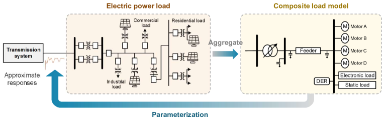
Figure 1: WECC CLM and its parameterization.

2.2 Parameterization Problem

WECC CLM parameterization is to properly choose the parameters for each type of aggregated models so that it’s capable of duplicating the dynamic behaviors of the detailed power loads, as seen in Figure 1. Measurement-based WECC CLM parameterization can be regarded as an inverse problem, the model parameters will be estimated according to the measurement data collected at the interconnection point of transmission system and the power loads, including active and reactive power trajectories, especially under fault disturbances, as formulated in (1).

$$y=F\left(\theta\right)\Rightarrow\theta={F^{-1}}\left(y\right)$$ (1)

where $F$ is the forward operator, ${F^{-1}}$ is inverse operator, $\theta$ denotes the model parameters, and $y$ is the measurement, as expressed by (2).

$$\begin{array}[]{l}y=[p,q]{\rm{}}\\ p=[{p_{\_}1},{p_{\_}2},\cdots,{p_{\_}T}]{\rm{}}\\ q=[{q_{\_}1},{q_{\_}2},\cdots,{q_{\_}T}]\end{array}$$ (2)

where $p$ and $q$ respectively represent the trajectories of active power and reactive power.

Baysian inference is a probabilistic approach to solve the inverse problem. It estimates the posterior distribution of parameters given prior information on model parameters based on Bayes’ theorem, as formulated by (3) (Murphy, 2012). The posterior distribution is proportional to the likelihood and the prior distribution as the occurrence probability will be known given a certain trajectory.

$$P\left({\theta|{y_{\_}0}}\right)=\frac{{P\left({{y_{\_}0}|\theta}\right)\cdot P\left(\theta\right)}}{{P\left({{y_{\_}0}}\right)}}\propto P\left({{y_{\_}0}|\theta}\right)\cdot P\left(\theta\right)$$ (3)

where $\theta$ is the model parameter, ${{y_{\_}0}}$ is the given trajectories, ${P\left(\theta\right)}$ and $P\left({\theta|{y_{\_}0}}\right)$ respectively represent the prior distribution and posterior distribution of model parameters, ${P\left({{y_{\_}0}|\theta}\right)}$ is the likelihood.

To solve the baysian inference problem, one classical approach is to sample the posterior distribution using Markov chain Monte Carlo (MCMC). Also, variational inference is another kind of idea that approximates the posterior within a parametric family of distributions (Nemani et al., 2023).

2.3 Probabilistic Diffusion Model

Diffusion model is an advanced generative model, that defines a Markov chain of diffusion steps to slowly add random noise to data, and then learn to reverse the diffusion process (Ho et al., 2020). It constructs new data samples from the noise by training with variational inference. Diffusion model belongs to the family of latent variable models and stands out due to its straightforward formulation, efficient training, and outstanding performance in generating high-quality samples. As an extension, conditional diffusion model allows for controlled generation of samples based on the additional inputs of conditions.

The diffusion process (forward process) is a parameterized Markov process from original data ${x_{\_}0}\sim q\left({{x_{\_}0}}\right)$ to the latent variable ${x_{\_}T}$. In each diffusion step, Gaussian noise is added to the original data, as expressed by (4).

$$q({x_{\_}{1:T}}|{x_{\_}0})=\prod\limits_{\_}{t=1}^{T}{q({x_{\_}t}|{x_{\_}{t-1}})},{\rm{}}q({x_{\_}t}|{x_{\_}{t-1}})=N({x_{\_}t};\sqrt{(1-{\beta_{\_}t})}{x_{\_}{t-1}},{\beta_{\_}t}I)$$ (4)

where $q({x_{\_}{1:T}}|{x_{\_}0})$ is an approximate posterior, $N\left({\mu,{\sigma^{2}}}\right)$ is a Gaussian distribution with mean $\mu$ and variance ${{\sigma^{2}}}$, ${\beta_{\_}1},{\beta_{\_}2},\cdots,{\beta_{\_}T}$ is the variance schedule of the noising process. Thus we have ${x_{\_}t}=\sqrt{(1-{\beta_{\_}t})}{x_{\_}{t-1}}+\sqrt{({\beta_{\_}t})}\varepsilon\;$ by sampling $\varepsilon\sim N\left(0,I\right)$.

The reverse process is defined as the joint distribution expressed by (5). It’s a Gaussian transition that gradually denoises the data from ${x_{\_}T}\sim N\left({0,I}\right)$, and finally achieve the real distribution $x_{\_}0$.

$${p_{\_}\theta}({x_{\_}{0:T}})=p({x_{\_}T})\prod\limits_{\_}{t=1}^{T}{{p_{\_}\theta}({x_{\_}{t-1}}|{x_{\_}t})},{\rm{}}{p_{\_}\theta}({x_{\_}{t-1}}|{x_{\_}t})=N({x_{\_}{t-1}};{\mu_{\_}\theta}({x_{\_}t},t),{\varepsilon_{\_}\theta}({x_{\_}t},t))$$ (5)

where ${\mu_{\_}\theta}({x_{\_}t},t)$ and ${\varepsilon_{\_}\theta}({x_{\_}t},t)$ respectively denote the parameterized mean and variance, which are approximated by the denoise neural network.

Training objective is to optimize the variational bound on negative log-likelihood of the joint distribution $p_{\_}\theta$ and $q$, which can also be transformed to the expression (6). Therefore, training the reverse process of diffusion model will be simplified to predict the Gaussian noise $\varepsilon$.

$$\min L\left(\theta\right)\Rightarrow\min{\mathbb{E}_{\_}{{x_{\_}0},\varepsilon}}{\left\|{\varepsilon-{\varepsilon_{\_}\theta}\left({\sqrt{{{\bar{\alpha}}_{\_}t}}{x_{\_}0}+\sqrt{1-{{\bar{\alpha}}_{\_}t}}\varepsilon,t}\right)}\right\|^{2}}$$ (6)

where ${\alpha_{\_}t}=1-{\beta_{\_}t}$, and ${{\bar{\alpha}}_{\_}t}=\prod\nolimits_{\_}{s=1}^{t}{{\alpha_{\_}s}}$.

3 JCDI Framework

Formulated WECC CLM parameterization as an inverse problem, we present JCDI, a novel framework that estimates WECC CLM parameters from measured power trajectories, as seen in Figure 2. JCDI employs the conditional diffusion model to capture the complex distributions among parameter space, and deduce the parameter posterior distribution given specific observations. Specifically, JCDI uses power trajectories as conditions to guide the diffusion process, and gradually refines parameter estimates through denoising. A denoise neural network structure, inverse grid transformer (IGT), is innovatively developed to predict the added noise in the denoise process. Therein, a transformer encoder is exploited to characterize the dependencies between different model parameters and power trajectories, and a multi-event joint conditioning scheme is incorporated to mitigate parameter degeneracy.

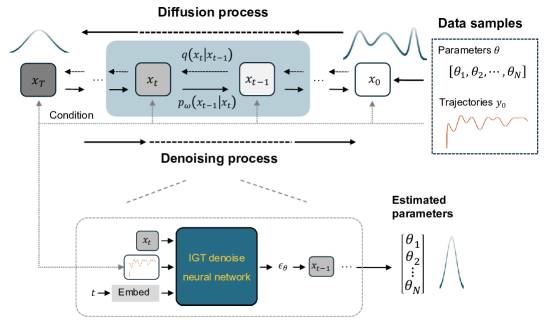
Figure 2: JCDI Framework.

3.1 IGT architecture

We design a novel denoise neural network named IGT based on transformer encoder, as presented in Figure 3. Transformer is a revolutionary neural network architecture in natural language processing. It converts the texts into numerical representations (tokens), and captures the long-range dependencies among different words in the context based on the attention mechanism (Vaswani et al., 2017). In our architecture, the transformer tokens are a concatenation of three types of inputs: 1) model parameters that are being denoised, 2) encoded power trajectories, 3) encoded diffusion time step $t$. All of them are tokenized with linear modules. The power trajectories act as the conditions, they are fed into the trajectory encoders, which employ Residual Network (ResNet) to extract trajectory features (He et al., 2016). The diffusion step $t$ is sinusoidally embedded, and included as a part of inputs for obtaining the diffusion step information for the diffusion model. The transformer encoder is composed a stack of multi-head attention followed with feed forward layers, and layer normalization is utilized for each sublayer. The attention model calculates the correlation of input elements (attention weight) and then produces the output representation by making weighted summation of the inputs: First, the input tokens are transformed into three variables, the query $Q$, key $K$, and value $V$, by multiplying their corresponding transformation matrices, as seen in (7). Next, the similarity between $Q$ and $K$ (the attention score), will be quantatized by their dot product, then it’s scaled by $\frac{1}{{\sqrt{{d_{\_}k}}}}$ and goes through softmax operation to obtain the attention weight. Finally the attention output is calculated by the weighted sum of value $V$, as expressed by (8). On this basis, the multi-head attention is implemented by performing several attention functions with different linear projections in parallel, and then concatenating the outputs. Therefore, the multi-head attention in this architecture is expected to represent the correlation among the unknown parameters of WECC CLM, as well as the relationship of model parameters and trajectory conditions, thus to improve the parameter estimation performance.

$$Q={W_{\_}Q}\cdot X,{\rm{}}K={W_{\_}K}\cdot X,{\rm{}}V={W_{\_}V}\cdot X$$ (7)

$${\rm{Attention}}\left({Q,K,V}\right)={\rm{softmax}}\left({\frac{{Q{K^{T}}}}{{\sqrt{{d_{\_}k}}}}}\right)\cdot V$$ (8)

where ${W_{\_}Q}$, ${W_{\_}K}$, and ${W_{\_}V}$ are the transformation matrices, $X$ represents the input tokens, and ${{d_{\_}k}}$ denotes the dimension of keys.

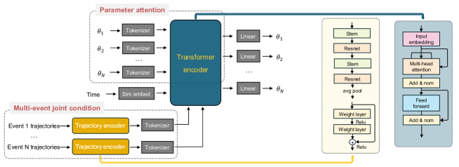
Figure 3: IGT architecture with multi-event joint condition.

3.2 Multi-event joint condition

Due to parameter degeneracy, the traditional parameter estimation methods using single disturbance may deduce various combinations of parameters, while some of them are not generalizable to other disturbances. Here, we address this challenge by the multi-event joint conditioning scheme: power trajectories under different fault events are input as the conditions to deduce model parameters simultaneously. Therefore, the posterior distribution of model parameters will be the joint probability that satisfies multiple trajectory conditions, which equals the product of individual ones due to the independence of fault events, as expressed by (LABEL:joint-condition). This serves to reduce parameter estimation uncertainties, thereby producing more robust and generalizable solutions. where ${y_{\_}{i,0}}$, $i$ = 1:$N$ denotes the measurement under the $i$-th fault event.

4 Simulation studies

4.1 Simulation settings

Model Configuration

To validate the proposed algorithm, WECC CLM is supplied by the IEEE 39-bus transmission system. The voltage profiles at bus 9 of the transmission system under different electric fault disturbances are fed into WECC CLM, and generate the system responses. In this work, three distinct fault events, including three-phase grounding bus faults that occur at bus 27, 5, 9 in the transmission system with fault clearing times of 135, 135, 44 ms, respectively, are selected to train the proposed JCDI. The selection of these specific fault events is motivated by the different dynamic behavior of the load system: Fault event 2 (FT_2) results in power electronic load tripping, Fault event 3 (FT_3) induces motor D stalling, while Fault event 1 (FT_1) exhibits neither phenomenon.

Parameter Selection

There are more than 100 unknown parameters in WECC CLM. Some of these parameters demonstrate significantly impact on the system dynamics, while others have a minor effect, and are difficult to estimate. To solve the parameterization problem efficiently and effectively, we conduct global sensitivity analysis with Sobol method across different fault events, and select 32 sensitive parameters for identification. The details of Sobol sensitivity analysis are presented in Appendix B.

Evaluation Metrics

To have a quantitative evaluation of the parameter identification result, two evaluation indices, that respectively measure the estimation accuracy of model parameters and power trajectories, are utilized in this paper.

For parameter estimation accuracy, the mean absolute percentage error (MAPE) is commonly used to measure the relative accuracy (de Myttenaere et al., 2016). However, it will become very large when the actual parameter value is close to zero. Therefore, we define a variant of MAPE, the mean absolute range percentage error (MARPE), to assess the parameter prediction accuracy, as expressed by (9). In MARPE, the absolute parameter errors are divided by the possible range of parameters, i.e., $UB-LB$, instead of the actual parameter value ${\theta_{\_}0}$. Therefore, the evaluation will not be affected by the values of actual parameters within the same range.

$$MARPE=100\frac{1}{N}\sum\limits_{\_}{i=1}^{N}{\left|{\frac{{\hat{\theta}-{\theta_{\_}0}}}{{UB-LB}}}\right|}$$ (9)

where ${\hat{\theta}}$ and ${{\theta_{\_}0}}$ respectively represent the estimated and actual values of parameters, $N$ is the number of parameters.

The trajectory accuracy is measured by the root mean squared error (RMSE) between the transient trajectories (including active power and reactive power) with the estimated parameters and the actual trajectories, as formulated by (10).

$$RMSE=\sqrt{\sum\nolimits_{\_}{t=1}^{T}{\frac{{{{\left({{p_{\_}{\hat{\theta}}}\left(t\right)-{p_{\_}0}\left(t\right)}\right)}^{2}}}}{T}+}}\sqrt{\sum\nolimits_{\_}{t=1}^{T}{\frac{{{{\left({{q_{\_}{\hat{\theta}}}\left(t\right)-{q_{\_}0}\left(t\right)}\right)}^{2}}}}{T}}}$$ (10)

where ${{p_{\_}{\hat{\theta}}}\left({t}\right)}$ and ${{q_{\_}{\hat{\theta}}}\left({t}\right)}$ respectively represent the estimated active and reactive powers at time $t$ , ${{p_{\_}0}\left({t}\right)}$ and ${{q_{\_}0}\left({t}\right)}$ are the actual active and reactive powers, $t$ is the time instant.

Dataset Generation

In the first stage of algorithm verification, we assume experts possess a priori domain knowledge regarding the model parameters, and the data to train and validate the algorithm is generated by conducting simulation with model parameters under uniform distribution within the range ${\theta_{\_}0}\pm 20\%\left({UB-LB}\right)$. ${\theta_{\_}0}$ represent the actual model parameters, $LB$ and $UB$ respectively denote the lower and upper bounds of model parameters, as listed in Table 3. The total dataset size is 250000, including 200000 samples for training, and 50000 for testing.

4.2 Results

A. Training progress

The proposed JCDI is trained for 5000 epochs until the training and testing losses level off. And then, the desired trajectory is injected to the well-trained model, and the model parameters are inferred probabilistically. The algorithm implementation details are explained in the Appendix C. In order to verify the effectiveness of multi-event joint conditioning, the proposed JCDI, which is conditioned on three fault events (FT_1, FT_2 and FT_3), is compared with CDI, the diffusion-based parameter estimation conditioned on a single event FT_1.

Figure 4 illustrates the training progress, including the evolution of losses and prediction errors for both CDI and JCDI. As the number of epochs increases, they decrease smoothly for both the training and testing sets. Compared with CDI, JCDI achieves lower final loss and smaller predicted parameter and trajectory errors. However, it is worth noting that even in the later stages of training, some predicted model parameters still deviate from their actual values, while the trajectory errors remain within a very small range. This suggests that the trained model can still accurately predict power trajectories even in the presence of these parameter deviations.

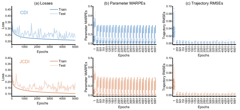
Figure 4: Evolution of losses and prediction errors during training.

B. Trajectory analysis

Substituting the inferred parameter sets into the WECC CLM, we deduce the post-fault trajectories under different fault events, as illustrated in Figure 5. We also calculate and compare the trajectory RMSEs in Figure 6. Under FT_1, the estimated active and reactive power trajectories under both CDI and JCDI closely match the actual trajectories. The mean trajectory RMSEs are approximately 0.001. Under FT_2, which involves electronic load tripping, the steady-state active power after the fault becomes smaller than its initial value due to incomplete load recovery. And under FT_3, which induces motor stalling, the absolute values of steady powers after the fault significantly increase. The estimated post-fault trajectories under CDI deviates substantially from the actual trajectories, with the mean trajectory RMSEs increasing to 0.0255 and 0.5503 for FT_2 and FT_3, respectively. In contrast, the power trajectories deduced by JCDI under FT_2 and FT_3 maintain high accuracy, with mean trajectory RMSEs of 0.0009 and 0.0061, respectively.

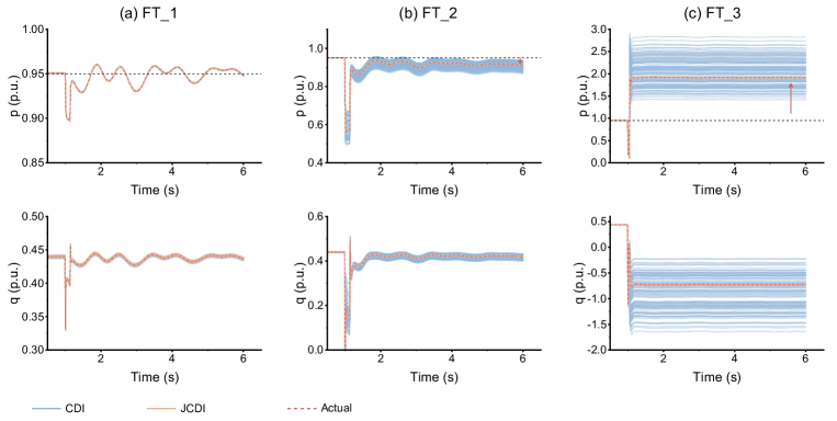
Figure 5: Post-fault trajectories with estimated parameters under different fault events.

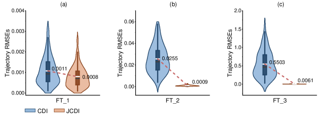
Figure 6: Comparison of trajectory RMSEs under different fault events.

C. Parameter analysis

Figure 7 compares the MARPEs of model parameters under CDI and JCDI. Under CDI, some model parameters, such as ${F_{\_}{{\rm{ma}}}}$, ${F_{\_}{{\rm{derA}}}}$, and ${K_{\_}{{\rm{p1}}}}$ can be accurately estimated, with MARPEs lower than 5%, while others exhibit significant uncertainties. This can be attributed to two factors. First, the parameter selection is based on a comprehensive sensitivity analysis under different fault events, hence some parameters to be identified are not sensitive under the fault event used in CDI. Second, parameter correlation, as presented in Figure 8, also contributes to the estimation uncertainty, as discussed in the following paragraph. Under JCDI, the parameter MARPEs of ${F_{\_}{{\rm{el}}}}$, ${F_{\_}{{\rm{md}}}}$, ${R_{\_}{{\rm{stall}}}}$, ${X_{\_}{{\rm{stall}}}}$, ${ComPF}$, ${f_{\_}{{\rm{rcel}}}}$, ${Q_{\_}{{\rm{el0}}}}$ are significantly reduced, as their sensitivities increase under fault events that induce electronic load tripping and motor stalling. Furthermore, the estimation accuracy of some other parameters, such as ${F_{\_}{{\rm{ma}}}}$, ${F_{\_}{{\rm{mb}}}}$, ${F_{\_}{{\rm{mc}}}}$, ${L_{\_}{{\rm{pA}}}}$, ${L_{\_}{{\rm{ppA}}}}$, ${L_{\_}{{\rm{pB}}}}$, ${L_{\_}{{\rm{ppB}}}}$, ${L_{\_}{{\rm{pC}}}}$, ${L_{\_}{{\rm{ppC}}}}$, is also effectively improved through the multi-event joint conditioning scheme in JCDI.

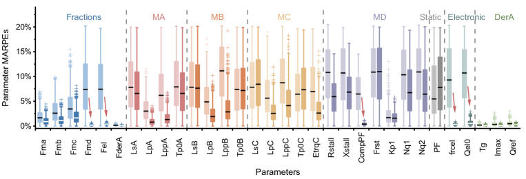
Figure 7: Comparison of parameter MARPEs.

Figure 8 illustrates the scatter plots of estimated model parameters, revealing strong correlations among several of them. For instance, the load fractions ${F_{\_}{{\rm{ma}}}}$ and ${F_{\_}{{\rm{mc}}}}$, ${F_{\_}{{\rm{mb}}}}$ and ${F_{\_}{{\rm{mc}}}}$, exhibit negative correlations. Conversely, the synchronous reactances and transient open circuit time constant of induction motors, namely ${L_{\_}{{\rm{sA}}}}$ and ${T_{\_}{{\rm{p0A}}}}$, ${L_{\_}{{\rm{sB}}}}$ and ${T_{\_}{{\rm{p0B}}}}$, ${L_{\_}{{\rm{sC}}}}$ and ${T_{\_}{{\rm{p0C}}}}$, demonstrate positive correlations. Notably, we find the terms ${L_{\_}{{\rm{sA(B,C)}}}}$/${T_{\_}{{\rm{p0A(B,C)}}}}$ appearing in the dynamic equation of induction motors (Ma et al., 2020), providing physical validation of the statistical correlations. Furthermore, ${L_{\_}{{\rm{pB}}}}$ for motor B is also positively related to ${L_{\_}{{\rm{pC}}}}$ for motor C. As a result, parameter combinations adhering to these correlation relationships will generate similar post-fault trajectories. This observation explains the aforementioned results, that we achieve high trajectory estimation accuracy despite high uncertainties in some model parameters.

When comparing JCDI with CDI, we find the multi-event joint conditioning employed in JCDI effectively reduces parameter uncertainties and thus enhances the parameter estimation accuracy. For example, there are high correlations of ${F_{\_}{{\rm{md}}}}$ and ${F_{\_}{{\rm{el}}}}$, ${L_{\_}{{\rm{pA}}}}$ and ${L_{\_}{{\rm{ppA}}}}$ under CDI, making it challenging to deduce the accurate parameters. However, under JCDI, the estimated parameters center around the actual values, which is exactly what to expect. Additionally, CDI fails to estimate ${R_{\_}{{\rm{stall}}}}$ and ${X_{\_}{{\rm{stall}}}}$, as they are not sensitive under FT_1. Nevertheless, JCDI reveals high correlations between ${R_{\_}{{\rm{stall}}}}$ and ${X_{\_}{{\rm{stall}}}}$, ${R_{\_}{{\rm{stall}}}}$ and ${F_{\_}{{\rm{rst}}}}$, ${X_{\_}{{\rm{stall}}}}$ and ${F_{\_}{{\rm{rst}}}}$.

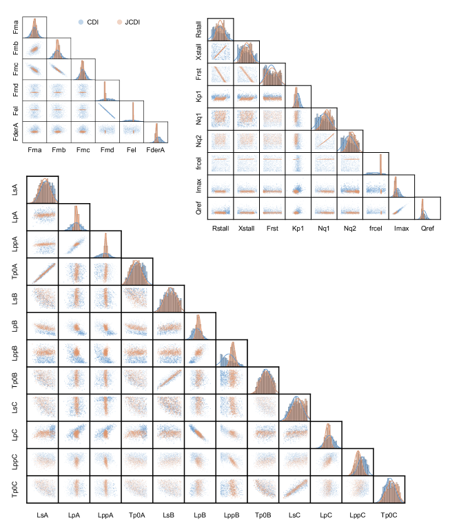
Figure 8: Scatter plots of estimated model parameters.

D. Generalizability performance

To verify the parameter generalizability across different fault events, we select three groups of additional scenarios to test the obtained parameter estimation results, including 100 ordinary fault events, 50 fault events that induce power electronic load tripping, and 10 fault events where motor D stalling occurs. Figure 9 compares the trajectory RMSEs under the selected testing events. For CDI, one single ordinary fault event is utilized to train the algorithm. The trajectory RMSEs under ordinary testing events are close to that of the training event, with a mean deviation of 0.97%. However, they vary significantly, ranging from 0.005 to 0.0271 under trip events, and increase to an average value of 0.548 under stall events. In contrast, for JCDI, the post-fault trajectories are accurately predicted under the testing events, the mean deviations are 0.35%, 1.91%, and 0.23% for the three testing groups, respectively.

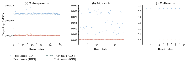
Figure 9: Trajectory RMSEs under three groups of testing fault events.

E. Algorithm comparison

To further demonstrate the superiority of proposed JCDI, different types of parameter estimation methods are compared, including:

• Reinforcement learning. We use reinforcement learning as a baseline because it’s extensively used for WECC CLM parameterization in the existing literature. It formulates the parameter estimation problem into a markov decision process (MDP). The agent modifies the model parameters according to the feedback of reward signals, thus moving towards the direction of reducing observation errors. Deep Q learning (DQN) is used in this study for comparison.

• Supervised learning. It learns the mapping from the observed trajectories to model parameters. Simliar with the neural network structure in JCDI, a trajectory encoder (ResNet) in series with a transformer encoder is used to infer the model parameters directly. Therefore, the comparison with supervised learning also serves as an ablation study demonstrating the necessity of the diffusion process.

The details of the comparative algorithms are described in Appendix C.

Table 1 compares the parameterization results under the aforementioned methods. The supervised learning methods deduce a deterministic result. The reinforcement learning and diffusion models provide a probabilistic solution, the mean errors, as well as the cases where the trajectory RMSE is minimal for FT_1 (treated as the best cases), are presented in the table. Under DQN, the agent aims to minimize the trajectory error by adjusting model parameters. However, it appears to track into local optimum: the estimated parameters still deviate a lot from the actual values, with a mean MARPE of 10.02%. The mean trajectory RMSE for FT_1 is 0.01, and it increase to 0.0216 and 0.3266, respectively for FT_2 and FT_3. For the best case, trajectory RMSE for FT_1 reduces to 0.0035, but the parameter MARPE remains large, and trajectory RMSEs increase significantly for FT_2 and FT_3. The supervised learning neural network (ResNet-Trans) achieves the smallest mean parameter MARPE of 3.27%, which aligns with its loss function. The trajectory RMSE under FT_1 is 0.004, and increases to 0.0074 and 0.2603, respectively under FT_2 and FT_3. Through the diffusion process, CDI generates a probabilistic solution set that encompasses various combinations of model parameters. This leads to the increase of parameter MARPE compared with ResNet-Trans. However, the trajectory RMSE using the estimated parameters derived from CDI reduces to 0.0011 under FT_1, indicating that the estimation result of CDI is much more comprehensive and precise. With the assistance of joint conditioning, JCDI further reduces the parameter estimation uncertainty, particularly for degenerate parameters. The mean parameter MARPE is reduced by 42.1% compared to CDI, and it achieves a high trajectory estimation accuracy across different fault events.

Table 1: Performance comparison of different parameterization methods

Algorithms	Parameter MARPEs	Trajectory RMSEs
		FT_1	FT_2	FT_3
DQN (mean)	10.02%	0.01	0.0217	0.3266
DQN (best)	10.05%	0.0035	0.0329	0.3878
ResNet-Trans	3.27%	0.004	0.0074	0.2603
CDI (mean)	6.51%	0.0011	0.0255	0.5503
CDI (best)	5.21%	1.06e-04	0.0273	0.6624
JCDI (mean)	3.77%	0.0008	0.0009	0.0061
JCDI (best)	3.04%	1.01e-04	2.71e-04	0.0067

F. Extended parameter range

So far we have evaluated the algorithms’ performance in a relatively narrow range of parameters $\pm$20% around their default values. It would be instructive to examine what happen if the parameter range is extended. In this case, data samples are generated under uniform distribution within $[LB,UB]$. Different parameterization methods are trained in the same way as the previous study except for the parameter range. Table 2 shows the parameterization results with the extended parameter range. Both of the mean parameter MARPEs and trajectory RMSEs are increased compared with the previous study. However, the diffusion models perform much better than other algorithms: the mean trajectory RMSEs for FT_1 are approximately 0.004 under CDI and JCDI, while they have been higher than 0.01 under DQN and ResNet-Trans. Also, the mean parameter MARPE under JCDI is further reduced by 26.3% compared with CDI, and JCDI achieves the lowest trajectory RMSEs for different fault events.

Table 2: Parameterization results with extended parameter range

Algorithms	Parameter MARPEs	Trajectory RMSEs
		FT_1	FT_2	FT_3
DQN (mean)	20.83%	0.018	0.0642	0.4272
DQN (best)	22.70%	0.0079	0.0594	0.2603
ResNet-Trans	11.98%	0.0158	0.0518	0.3794
CDI (mean)	18.08%	0.0042	0.0787	0.8724
CDI (best)	18.29 %	6.345e-04	0.0936	0.8874
JCDI (mean)	13.33%	0.0041	0.0043	0.0180
JCDI (best)	14.35 %	4.25e-04	0.0018	0.0085

5 Conclusion

In this work, we present JCDI, a novel probabilistic parameter estimation framework that addresses the key challenges of parameter degeneracy and cross-event generalization through the multi-event joint conditioning structure and transformer encoder-based denoise neural network. Successful verification of JCDI has been achieved for WECC CLM in power systems. Our comprehensive evaluation yields several key findings. First, the global sensitivity analysis reveals the sensitivity discrepancies under different fault events, particularly when power electronic load tripping or motor stalling occurs. Second, single-event parameterization produces multiple valid parameter sets that accurately model power trajectories - but only for the specific disturbance, demonstrating the degeneracy property in WECC CLM. Third, JCDI enhances parameter estimation accuracy in these degenerate cases. The parameters derived by JCDI accurately reproduce power trajectories under a group of fault events. Finally, comparative studies firmly establish JCDI’s superiority over existing parameter estimation methods, including deep reinforcement learning and supervised neural networks. Beyond load modeling application, the proposed JCDI can also be extended to other electric systems, such as power electronic converters and energy storage systems, as well as other research fields.

Appendix A Mathematical model and characteristics of WECC CLM

This appendix introduces the mathematical model and electrical characteristics of each component in WECC CLM. Each component is specified by a certain fraction (${F_{\_}{ma}}$, ${F_{\_}{mb}}$, ${F_{\_}{mc}}$, ${F_{\_}{md}}$, ${F_{\_}{el}}$, ${F_{\_}{derA}}$ for fractions of motors A, B, C, D, power electronic load, and DER, respectively, and the remainder for static load), and the individual responses are summed together to represent the overall performance of electric loads.

Three-Phase Induction Motors:

WECC CLM categories the three-phase induction motors into motors A, B and C. They are modeled by fifth-order differential-algebraic equations based on electromagnetic equations and electromechanical equations with different parameters (Ma et al., 2020). Motor A characterizes the three-phase induction motors that drive low inertia constant torque loads, typical examples include positive displacement compressors and pumps (EPR, September 2020). Motor B represent the high inertia variable torque loads, such as large fans, and motor C is used to model the low inertia variable torque loads, such as centrifugal pumps.

Single-Phase Induction Motor:

Motor D represents the single-phase induction motor, such as residential air-conditioners and heat ventilation. In WECC CLM, it’s developed as a "performance model" based on laboratory test. One important characteristic for the single-phase induction motor is the stalling behavior during voltage dips, that is, there is insufficient motor torque to overcome the load torque and therefore the motor stops. Figure 10 shows the power change of motor D during the stalling and recovering processes.

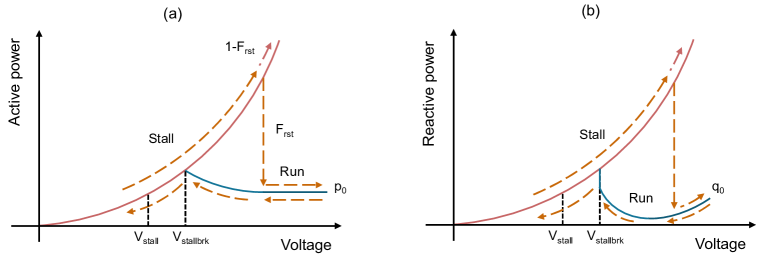
Figure 10: The power changes of motor D when stalling.

When the voltage remains above the motor compressor breakdown voltage, i.e. $V>{V_{\_}{brk}}$, the motor works in run state, and the active and reactive powers are expressed by (35).

$$\begin{array}[]{l}p=\left({{p_{\_}0}+{K_{\_}{p1}}\cdot{{\left({V-{V_{\_}{brk}}}\right)}^{{N_{\_}{p1}}}}}\right)\cdot\left({1+CmpKpf\cdot\Delta f}\right)\\ q=\left({{q_{\_}0}+{K_{\_}{q1}}\cdot{{\left({V-{V_{\_}{brk}}}\right)}^{{N_{\_}{q1}}}}}\right)\cdot\left({1+CmpKqf\cdot\Delta f}\right)\end{array}$$ (35)

where $p$ and $q$ are the active and reactive powers of motor D, ${p_{\_}0}$ and ${q_{\_}0}$ are the initial powers. $V$ denotes the terminal voltage, $\Delta f$ represents the frequency deviation. ${K_{\_}{p1}}$ and ${K_{\_}{q1}}$ are the voltage coefficients, ${N_{\_}{p1}}$ and ${N_{\_}{q1}}$ are the power exponents, $CmpKpf$ and $CmpKqf$ are the frequency coefficients.

When the voltage reduces between ${V_{\_}{brk}}$ and the motor stalling voltage ${V_{\_}{stall}}$, motor D still works in run state, but the expressions of powers are formulated as (38).

$$\begin{array}[]{l}p=\left({{p_{\_}0}+{K_{\_}{p2}}\cdot{{\left({{V_{\_}{brk}}-V}\right)}^{{N_{\_}{p2}}}}}\right)\cdot\left({1+CmpKpf\cdot\Delta f}\right)\\ q=\left({{q_{\_}0}+{K_{\_}{q2}}\cdot{{\left({{V_{\_}{brk}}-V}\right)}^{{N_{\_}{q2}}}}}\right)\cdot\left({1+CmpKqf\cdot\Delta f}\right)\end{array}$$ (38)

where ${K_{\_}{p2}}$ and ${K_{\_}{q2}}$ are the voltage coefficients, ${N_{\_}{p2}}$ and ${N_{\_}{q2}}$ are the power exponents.

When the voltage drops lower than ${V_{\_}{stall}}$ for a time duration of ${T_{\_}{stall}}$, motor D transitions to stall state, and the active and reactive powers are calculated by (41).

$$\begin{array}[]{l}p={V^{2}}/{R_{\_}{stall}}\\ q=-{V^{2}}/{X_{\_}{stall}}\end{array}$$ (41)

where ${R_{\_}{stall}}$ and ${X_{\_}{stall}}$ respectively denote the stall resistance and reactance.

Finally, when the voltage recovers and becomes higher than the restarting voltage ${V_{\_}{rst}}$ of the stalled motors for a time duration of ${T_{\_}{rst}}$, a portion (${F_{\_}{rst}}$) of the motor D loads transitions to run state, while the rest remains in stall state.

Therefore, it’s noticed from (41) that the powers of motor D are proportional to the square of voltage in stall state, leading to a high power consumption during voltage recovery.

Static Load Model:

The ZIP model, which consists of constant impedance (Z), constant current (I) and constant power (P) components, is used to represent the static loads. The active and reactive powers are time independent, their relationship with voltage is expressed by (44).

$$\begin{array}[]{l}p={p_{\_}0}\cdot\left({{p_{\_}{1c}}\cdot{{\left({\frac{V}{{{V_{\_}0}}}}\right)}^{{p_{\_}{1e}}}}+{p_{\_}{2c}}\cdot{{\left({\frac{V}{{{V_{\_}0}}}}\right)}^{{p_{\_}{2e}}}}+{p_{\_}3}}\right)\cdot\left({1+{p_{\_}{frq}}\cdot\Delta f}\right)\\ q={q_{\_}0}\cdot\left({{q_{\_}{1c}}\cdot{{\left({\frac{V}{{{V_{\_}0}}}}\right)}^{{q_{\_}{1e}}}}+{q_{\_}{2c}}\cdot{{\left({\frac{V}{{{V_{\_}0}}}}\right)}^{{q_{\_}{2e}}}}+{q_{\_}3}}\right)\cdot\left({1+{q_{\_}{frq}}\cdot\Delta f}\right)\end{array}$$ (44)

where ${p_{\_}0}$ and ${q_{\_}0}$ are the initial active and reactive powers of static load, which are calculated by (47), ${V_{\_}0}$ is the initial terminal voltage. ${p_{\_}{1c}}$, ${q_{\_}{1c}}$, ${p_{\_}{2c}}$ and ${q_{\_}{2c}}$ are power coefficients. ${p_{\_}{3}}$ and ${q_{\_}{3}}$ are the percentages of constant power loads, as calculated by (50). ${p_{\_}{frq}}$ and ${q_{\_}{frq}}$ are the frequency sensitivities of active and reactive powers.

$$\begin{array}[]{l}{p_{\_}0}={p_{\_}{load}}\cdot\left({1-{F_{\_}{ma}}-{F_{\_}{mb}}-{F_{\_}{mc}}-{F_{\_}{md}}-{F_{\_}{el}}-{F_{\_}{derA}}}\right)\\ {q_{\_}0}={p_{\_}0}\cdot\tan\left({{\rm{acos}}\left({PF}\right)}\right)\end{array}$$ (47)

where ${p_{\_}{load}}$ represents the total active power of WECC CLM, $PF$ represents the power factor of static load.

$$\begin{array}[]{l}{p_{\_}3}=1-{p_{\_}{1c}}-{p_{\_}{2c}}\\ {q_{\_}3}=1-{q_{\_}{1c}}-{q_{\_}{2c}}\end{array}$$ (50)

Power Electronic Load:

The power electronic load in WECC CLM represents an aggregation of inverter-interfaced or electronic coupled loads, such as consumer electronic devices like computers. The power-voltage relationship of electronic load is shown in Figure 11. When the voltage maintains above ${V_{\_}{d1}}$, it consumes constant active and reactive power. When the voltage drops lower than ${V_{\_}{d1}}$, the electronic loads start to trip and the powers reduce linearly with voltage until 0. The active and reactive powers will also recover gradually with voltage but with a certain fraction.

Figure 11: The characteristic of power electronic load with tripping.

DER:

Distributed energy resource model version A (DER_A) is newly developed in load modeling to represent the aggregation of inverter-based generation (e.g. photovoltaic) (CMP, Feburary 2015). Its block diagram and specification refers to (DER, 2019). Compared with the previous DER model pvd1, DER_A has more functionalities, such as various control modes, thus can represent various distributed generation (DG) models to be plugged into WECC CLM.

Appendix B Sobol global sensitivity analysis

In this work, sensitivity analysis based on Sobol’s method (Sobol, 2001; Tosin et al., 2020; Saltelli, 2002; Iwanaga et al., 2022; Herman and Usher, 2017) is conducted for parameter reduction. Sobol’s method is a variance-based global sensitivity analysis method, which decomposes the variance of output into contributions from individual input parameters and their interactions.

First order index measures the individual effect of the input variable ${{X_{\_}i}}$ on the output, as defined by (51).

$${S_{\_}i}=\frac{{Va{r_{\_}{{X_{\_}i}}}\left({{E_{\_}{{X_{\_}{\sim i}}}}\left({Y|{X_{\_}i}}\right)}\right)}}{{Var\left(Y\right)}}$$ (51)

where $Y$ is the output of the model, ${Var\left(Y\right)}$ denotes the variance of the output. ${{X_{\_}i}}$ is the $i-$th input variable, ${{X_{\_}{\sim i}}}$ represents the set of all variables except ${{X_{\_}i}}$, and ${{E_{\_}{{X_{\_}{\sim i}}}}\left({Y|{X_{\_}i}}\right)}$ represents the expectation of $Y$ conditioned on a certain value of ${{X_{\_}{\sim i}}}$.

Second order index indicates the effect of interaction between ${{X_{\_}i}}$ and ${{X_{\_}j}}$, as expressed by

$${S_{\_}{ij}}=\frac{{Var\left({{M_{\_}{ij}}\left({{X_{\_}{ij}}}\right)}\right)}}{{Var\left(Y\right)}}$$ (52)

Total order index calculates the full contribution of the input variable ${{X_{\_}i}}$ on the output variance. Therefore, it’s summed by the sobol indices of different orders related to ${{X_{\_}i}}$, as expressed by (53).

$${S_{\_}{Ti}}=\sum\limits_{\_}{i\in u}{{S_{\_}u}}$$ (53)

To have a better understanding of the sensitivity differences for different fault events, the Sobol indices of parameters in WECC CLM are calculated respectively under FT_1, FT_2 and FT_3, as seen in Figure 13, and the model parameters are ranked according to the total Sobol indices in Figure  12.

Most of the parameters have similar sensitivity under different fault events. However, under FT_2, when the power electronic load trips, $frcel$ becomes much more sensitive than that under FT_1, and the sensitivities of ${F_{\_}{el}}$, $CompPF$ also get increased. Similarly, under FT_3, with the occurrence of motor D stalling, ${F_{\_}{md}}$ becomes the most sensitive parameter, whose sensitivity is significantly larger than other parameters. Besides, parameters including ${L_{\_}{sc}}$, ${R_{\_}{stall}}$, ${X_{\_}{stall}}$ and ${F_{\_}{rst}}$ have higher sensitivity than under FT_1. Comprehensively considering the sensitivity rankings under the three fault events, 32 sensitive parameters are selected for parameter estimation. They are listed in Table 3.

Figure 12: The ranking of parameter sensitivity under different fault events.

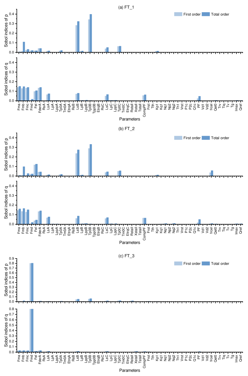
Figure 13: Sobol indices of parameters in WECC CLM.

Table 3: List of selected sensitive parameters

Notations	Description	Ranges	Default values
${F_{\_}{ma}}$	Motor A fraction	[0,0.5]	0.15
${F_{\_}{mb}}$	Motor B fraction	[0,0.5]	0.15
${F_{\_}{mc}}$	Motor C fraction	[0,0.5]	0.15
${F_{\_}{md}}$	Motor D fraction	[0,0.5]	0.15
${F_{\_}{el}}$	Electronic load fraction	[0,0.5]	0.25
${F_{\_}{derA}}$	derA fraction	[0,0.5]	0.15
${L_{\_}{sA}}$	Synchronous reactance (pu) of motor A	[0.9,3.6]	1.8
${L_{\_}{pA}}$	Transient reactance (pu) of motor A	[0.05,0.2]	0.1
${L_{\_}{ppA}}$	Subtransient reactance (pu) of motor A	[0.042,0.168]	0.083
${T_{\_}{p0A}}$	Transient open circuit time constant (sec.) of motor A	[0.046,0.184]	0.092
${L_{\_}{sB}}$	Synchronous reactance (pu) of motor B	[0.9,3.6]	1.8
${L_{\_}{pB}}$	Transient reactance (pu) of motor B	[0.08,0.32]	0.16
${L_{\_}{ppB}}$	Subtransient reactance (pu) of motor B	[0.06,0.24]	0.12
${T_{\_}{p0B}}$	Transient open circuit time constant (sec.) of motor B	[0.05,0.2]	0.1
${L_{\_}{sC}}$	Synchronous reactance (pu) of motor C	[0.9,3.6]	1.8
${L_{\_}{pC}}$	Transient reactance (pu) of motor C	[0.08,0.32]	0.16
${L_{\_}{ppC}}$	Subtransient reactance (pu) of motor C	[0.06,0.24]	0.12
${T_{\_}{p0C}}$	Transient open circuit time constant (sec.) of motor C	[0.05,0.2]	0.1
${E_{\_}{trqC}}$	Speed exponent for mechanical toque of motor C	[1,4]	2
${R_{\_}{stall}}$	Stall resistance (pu) of motor D	[0.08,0.12]	0.1
${X_{\_}{stall}}$	Stall reactance (pu) of motor D	[0.08,0.12]	0.1
${CompPF}$	Power factor of motor D	[0.8,1]	0.98
${F_{\_}{rst}}$	Fraction of load that can restart after stalling of motor D	[0.1,0.3]	0.2
${K_{\_}{p1}}$	Active power coefficient of motor D	[-1,1]	0
${N_{\_}{q1}}$	Reactive power exponent of motor D	[1,4]	2
${PF}$	Power factor of static load	[0.8,1]	0.99
${f_{\_}{rcel}}$	Fraction of electronic load that recovers from low voltage trip	[0,0.8]	0.75
${Q_{\_}{el0}}$	Initial value of ${Q_{\_}{el}}$	[0.4,0.6]	0.5
${T_{\_}{g}}$	Current control time constant (s)	[0.01,0.04]	0.02
${I_{\_}{max}}$	Maximum converter current (pu)	[1.1,1.3]	1.2
${Q_{\_}{ref}}$	Reactive power reference of derA (pu)	[0.5,0.9]	0.5

Appendix C Algorithm settings

JCDI

The algorithm and training parameters for the proposed JCDI are listed in Table 4. The transformer encoder includes 3 layers and 4 attention heads. There are 2 Resnet blocks and 3 Stem blocks in the trajectory encoder. For the diffusion process, the diffusion step is 200, and a linear variance schedule is used to add noise. Adam Optimizer is used to minimize the loss function, with a learning rate of $1\times{10^{-4}}$, and a batch size of 128. Training is implemented with Pytorch on a NVIDIA GeForce RTX 3090 graphics processing unit (GPU).

Table 4: Hyperparameters of JCDI

Parameter types	Hyperparameters	Notations	Values
Diffusion model	Diffusion step	$T$	200
	Initial value of variance schedule	${\beta_{\_}0}$	0.0001
	Final value of variance schedule	${\beta_{\_}T}$	0.005
Training	Batch size	$B$	128
	Learning rate	$lr$	$1\times{10^{-4}}$
Trajectory encoder	Resnet blocks	-	2
	Stem blocks	-	3
	Stem configurations (features, kernel size, padding, stride)	-	(32,4,0,4)
			(128,4,1,2)
			(256,4,1,2)
Transformer encoder	Number of heads	-	4
	Number of layers	-	3
	Features in the input	-	256
	Features in the feed-forward network	-	512

Supervised learning

The neural network structure for supervised learning is presented in Figure  14. The active and reactive power trajectories are input to the ResNet-based trajectory encoder, which extracts the features of the trajectories. The output features are then tokenized and input into the transformer encoder, based on which the model parameters are inferenced. The algorithm parameters are listed in Table 5.

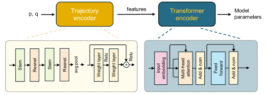
Figure 14: The neural network structure for supervised learning.

Table 5: Hyperparameters for supervised learning

Parameter types	Hyperparameters	Notations	Values
Training	Batch size	$B$	128
	Initial learning rate	$lr$	$1\times{10^{-4}}$
	Learning rate decay schedule	-	$\times 0.5$, at epochs: [50,100,150,200]
Trajectory encoder	Resnet blocks	-	2
	Stem blocks	-	3
	Stem configurations (features, kernel size, padding, stride)	-	(32,4,0,3)
			(128,4,1,1)
			(256,4,1,1)
Transformer encoder	Number of heads	-	4
	Number of layers	-	3
	Features in the input	-	256
	Features in the feed-forward network	-	512

Reinforcement learning

Formulated the parameter calibration process for WECC CLM as a MDP, the agent starts from an initial parameter estimation state, modifies the parameters at each step, transfers to the next state of estimation, calculates the reward according to the change of RMSE, and finally learns a policy that is able to adjust the WECC CLM parameters in the direction of minimizing RMSEs of dynamic responses. Therefore, the state is defined as the current estimation of parameters, as expressed by (118).

$$s=\hat{\theta}$$ (118)

Action is defined as the adjustment of parameters, as expressed by (119).

$$a=\Delta\hat{\theta}$$ (119)

State transition represents the parameter update, as represented by (120).

$$s^{\prime}=\hat{\theta}^{\prime}=\hat{\theta}+\Delta\hat{\theta}$$ (120)

Reward is calculated according to the decrement of trajectory RMSE in (10). To motivate continuous accuracy improvement when RMSE is small, a reciprocal respresentation is used, as seen in (121).

$$r=-\Delta\frac{{1}}{{RMSE{\rm{+}}0.1}}$$ (121)

We use deep Q learning (DQN) to solve the parameterization problem Mnih et al. (2015). DQN is a value-based RL method, that updates the action-value function (Q function) by the temporal difference approach, as expressed by (122). In this work, the Q function is approximated by a fully connected neural network, which has 2 hidden layers with 512 and 256 units, respectively. The $\varepsilon$-greedy policy with a piecewise exploration schedule is used to realize the trade-off between exploration and exploitation. The training parameters for DQN are listed in Table 6.

$${Q\left({s^{\prime},a}\right)=Q\left({s,a}\right)+\alpha\cdot\left({r^{\prime}+\gamma\cdot{{\max}_{\_}a}Q\left({s^{\prime},a}\right)\left.{-Q\left({s,a}\right)}\right)}\right.}$$ (122)

where $Q\left({s,a}\right)$ denotes the action-value function, $\alpha$ is the learning rate.

Table 6: Hyperparameters of DQN

Hyperparameters	Notations	Values
Learning rate	$lr$	$1\times{10^{-3}}\to 5\times{10^{-5}}$
Batch size	$B$	32
Replay buffer size	${B_{\_}r}$	5000
Target update frequency	${f_{\_}T}$	500

References

- Wang et al. [2023] Hanchen Wang, Tianfan Fu, Yuanqi Du, Wenhao Gao, Kexin Huang, Ziming Liu, Payal Chandak, Shengchao Liu, Peter Van Katwyk, Andreea Deac, et al. Scientific discovery in the age of artificial intelligence. Nature, 620(7972):47–60, 2023.
- Kadeethum et al. [2021] Teeratorn Kadeethum, Daniel O’Malley, Jan Niklas Fuhg, Youngsoo Choi, Jonghyun Lee, Hari S Viswanathan, and Nikolaos Bouklas. A framework for data-driven solution and parameter estimation of pdes using conditional generative adversarial networks. Nature Computational Science, 1(12):819–829, 2021.
- Lederman et al. [2021] Dylan Lederman, Raghav Patel, Omar Itani, and Horacio G. Rotstein. Parameter estimation in the age of degeneracy and unidentifiability. bioRxiv, 2021. doi:10.1101/2021.11.28.470243. URL https://www.biorxiv.org/content/early/2021/11/28/2021.11.28.470243.
- Kim et al. [2023] Jae-Kyeong Kim, Jiseong Kang, Jae Woong Shim, Heejin Kim, Jeonghoon Shin, Chongqing Kang, and Kyeon Hur. Dynamic performance modeling and analysis of power grids with high levels of stochastic and power electronic interfaced resources. Proceedings of the IEEE, 111(7):854–872, 2023. doi:10.1109/JPROC.2023.3284890.
- NER [December 2016] Technical reference document: Dynamic load modeling. Technical report, North American Electric Reliability Corporation (NERC) Load Modeling Task Force, December 2016.
- WEC [April 2021] Wecc composite load model specification technical report. Technical report, Western Electricity Coordinating Council (WECC), April 2021.
- Wang and Wang [2014] Zhaoyu Wang and Jianhui Wang. Time-varying stochastic assessment of conservation voltage reduction based on load modeling. IEEE Transactions on Power Systems, 29(5):2321–2328, 2014.
- Wang et al. [2020] Xinan Wang, Yishen Wang, Di Shi, Jianhui Wang, and Zhiwei Wang. Two-stage wecc composite load modeling: A double deep q-learning networks approach. IEEE Transactions on Smart Grid, 11(5):4331–4344, 2020. doi:10.1109/TSG.2020.2988171.
- Bu et al. [2020] Fankun Bu, Zixiao Ma, Yuxuan Yuan, and Zhaoyu Wang. Wecc composite load model parameter identification using evolutionary deep reinforcement learning. IEEE Transactions on Smart Grid, 11(6):5407–5417, 2020. doi:10.1109/TSG.2020.3008730.
- Xie et al. [2021a] Jian Xie, Zixiao Ma, Kaveh Dehghanpour, Zhaoyu Wang, Yishen Wang, Ruisheng Diao, and Di Shi. Imitation and transfer q-learning-based parameter identification for composite load modeling. IEEE Transactions on Smart Grid, 12(2):1674–1684, 2021a. doi:10.1109/TSG.2020.3025509.
- Afrasiabi et al. [2023] Shahabodin Afrasiabi, Mousa Afrasiabi, Mohammad Amin Jarrahi, Mohammad Mohammadi, Jamshid Aghaei, Mohammad Sadegh Javadi, Miadreza Shafie-Khah, and João P. S. Catalão. Wide-area composite load parameter identification based on multi-residual deep neural network. IEEE Transactions on Neural Networks and Learning Systems, 34(9):6121–6131, 2023. doi:10.1109/TNNLS.2021.3133350.
- Hu et al. [2023a] Jianxiong Hu, Qi Wang, Yujian Ye, and Yi Tang. Toward online power system model identification: A deep reinforcement learning approach. IEEE Transactions on Power Systems, 38(3):2580–2593, 2023a. doi:10.1109/TPWRS.2022.3180415.
- Khodayar and Wang [2021] Mahdi Khodayar and Jianhui Wang. Probabilistic time-varying parameter identification for load modeling: A deep generative approach. IEEE Transactions on Industrial Informatics, 17(3):1625–1636, 2021. doi:10.1109/TII.2020.2971014.
- Khazeiynasab et al. [2022] Seyyed Rashid Khazeiynasab, Junbo Zhao, and Nan Duan. Wecc composite load model parameter identification using deep learning approach. In 2022 IEEE Power & Energy Society General Meeting (PESGM), pages 1–5, 2022. doi:10.1109/PESGM48719.2022.9916921.
- Tan et al. [2024] Bendong Tan, Junbo Zhao, and Nan Duan. Amortized bayesian parameter estimation approach for wecc composite load model. IEEE Transactions on Power Systems, 39(1):1517–1529, 2024. doi:10.1109/TPWRS.2023.3250579.
- Hu et al. [2023b] Jianxiong Hu, Qi Wang, Yujian Ye, and Yi Tang. Toward online power system model identification: A deep reinforcement learning approach. IEEE Transactions on Power Systems, 38(3):2580–2593, 2023b. doi:10.1109/TPWRS.2022.3180415.
- Xie et al. [2021b] Jian Xie, Zixiao Ma, Kaveh Dehghanpour, Zhaoyu Wang, Yishen Wang, Ruisheng Diao, and Di Shi. Imitation and transfer q-learning-based parameter identification for composite load modeling. IEEE Transactions on Smart Grid, 12(2):1674–1684, 2021b. doi:10.1109/TSG.2020.3025509.
- Cao et al. [2023] Yihan Cao, Siyu Li, Yixin Liu, Zhiling Yan, Yutong Dai, Philip S Yu, and Lichao Sun. A comprehensive survey of ai-generated content (aigc): A history of generative ai from gan to chatgpt. arXiv preprint arXiv:2303.04226, 2023.
- Zhang et al. [2023] Chaoning Zhang, Chenshuang Zhang, Sheng Zheng, Yu Qiao, Chenghao Li, Mengchun Zhang, Sumit Kumar Dam, Chu Myaet Thwal, Ye Lin Tun, Le Luang Huy, et al. A complete survey on generative ai (aigc): Is chatgpt from gpt-4 to gpt-5 all you need? arXiv preprint arXiv:2303.11717, 2023.
- Ho et al. [2020] Jonathan Ho, Ajay Jain, and Pieter Abbeel. Denoising diffusion probabilistic models. Advances in neural information processing systems, 33:6840–6851, 2020.
- Du et al. [2023] Hongyang Du, Ruichen Zhang, Yinqiu Liu, Jiacheng Wang, Yijing Lin, Zonghang Li, Dusit Niyato, Jiawen Kang, Zehui Xiong, Shuguang Cui, et al. Beyond deep reinforcement learning: A tutorial on generative diffusion models in network optimization. arXiv preprint arXiv:2308.05384, 2023.
- Yang et al. [2023] Ling Yang, Zhilong Zhang, Yang Song, Shenda Hong, Runsheng Xu, Yue Zhao, Wentao Zhang, Bin Cui, and Ming-Hsuan Yang. Diffusion models: A comprehensive survey of methods and applications. ACM Computing Surveys, 56(4):1–39, 2023.
- Kawar et al. [2022] Bahjat Kawar, Michael Elad, Stefano Ermon, and Jiaming Song. Denoising diffusion restoration models. Advances in Neural Information Processing Systems, 35:23593–23606, 2022.
- Daras et al. [2024] Giannis Daras, Hyungjin Chung, Chieh-Hsin Lai, Yuki Mitsufuji, Jong Chul Ye, Peyman Milanfar, Alexandros G. Dimakis, and Mauricio Delbracio. A survey on diffusion models for inverse problems, 2024. URL https://arxiv.org/abs/2410.00083.
- Murphy [2012] Kevin P Murphy. Machine learning: a probabilistic perspective. MIT press, 2012.
- Nemani et al. [2023] Venkat Nemani, Luca Biggio, Xun Huan, Zhen Hu, Olga Fink, Anh Tran, Yan Wang, Xiaoge Zhang, and Chao Hu. Uncertainty quantification in machine learning for engineering design and health prognostics: A tutorial. Mechanical Systems and Signal Processing, 205:110796, 2023.
- Vaswani et al. [2017] Ashish Vaswani, Noam Shazeer, Niki Parmar, Jakob Uszkoreit, Llion Jones, Aidan N Gomez, Lukasz Kaiser, and Illia Polosukhin. Attention is all you need.(nips), 2017. arXiv preprint arXiv:1706.03762, 10:S0140525X16001837, 2017.
- He et al. [2016] Kaiming He, Xiangyu Zhang, Shaoqing Ren, and Jian Sun. Deep residual learning for image recognition. In Proceedings of the IEEE conference on computer vision and pattern recognition, pages 770–778, 2016.
- de Myttenaere et al. [2016] Arnaud de Myttenaere, Boris Golden, Bénédicte Le Grand, and Fabrice Rossi. Mean absolute percentage error for regression models. Neurocomputing, 192:38–48, June 2016. ISSN 0925-2312. doi:10.1016/j.neucom.2015.12.114. URL http://dx.doi.org/10.1016/j.neucom.2015.12.114.
- Ma et al. [2020] Zixiao Ma, Zhaoyu Wang, Yishen Wang, Ruisheng Diao, and Di Shi. Mathematical representation of wecc composite load model. Journal of Modern Power Systems and Clean Energy, 8(5):1015–1023, 2020.
- EPR [September 2020] Technical reference on the composite load model. Technical report, The Electric Power Research Institute (EPRI), September 2020.
- CMP [Feburary 2015] Wecc composite load model with dg specification. Technical report, Western Electricity Coordinating Council (WECC), Feburary 2015.
- DER [2019] The new aggregated distributed energy resources (dera) model for transmission planning studies: 2019 update. Technical report, Electric Power Research Institute, 2019.
- Sobol [2001] I.M Sobol. Global sensitivity indices for nonlinear mathematical models and their monte carlo estimates. Mathematics and Computers in Simulation, 55(1):271–280, 2001. ISSN 0378-4754. doi:https://doi.org/10.1016/S0378-4754(00)00270-6. URL https://www.sciencedirect.com/science/article/pii/S0378475400002706. The Second IMACS Seminar on Monte Carlo Methods.
- Tosin et al. [2020] Michel Tosin, Adriano MA Côrtes, and Americo Cunha. A tutorial on sobol’global sensitivity analysis applied to biological models. Networks in Systems Biology: Applications for Disease Modeling, pages 93–118, 2020.
- Saltelli [2002] Andrea Saltelli. Making best use of model evaluations to compute sensitivity indices. Computer Physics Communications, 145(2):280–297, 2002. ISSN 0010-4655. doi:https://doi.org/10.1016/S0010-4655(02)00280-1. URL https://www.sciencedirect.com/science/article/pii/S0010465502002801.
- Iwanaga et al. [2022] Takuya Iwanaga, William Usher, and Jonathan Herman. Toward SALib 2.0: Advancing the accessibility and interpretability of global sensitivity analyses. Socio-Environmental Systems Modelling, 4:18155, May 2022. doi:10.18174/sesmo.18155. URL https://sesmo.org/article/view/18155.
- Herman and Usher [2017] Jon Herman and Will Usher. SALib: An open-source python library for sensitivity analysis. The Journal of Open Source Software, 2(9), jan 2017. doi:10.21105/joss.00097. URL https://doi.org/10.21105/joss.00097.
- Mnih et al. [2015] Volodymyr Mnih, Koray Kavukcuoglu, David Silver, Andrei A Rusu, Joel Veness, Marc G Bellemare, Alex Graves, Martin Riedmiller, Andreas K Fidjeland, Georg Ostrovski, et al. Human-level control through deep reinforcement learning. nature, 518(7540):529–533, 2015.