Simulating the two-dimensional $t-J$ model at finite doping
with neural quantum states

Abstract

Simulating large, strongly interacting fermionic systems remains a major challenge for existing numerical methods. In this work, we present, for the first time, the application of neural quantum states – specifically, hidden fermion determinant states (HFDS) – to simulate the strongly interacting limit of the Fermi-Hubbard model, namely the $t-J$ model, across the entire doping regime. We demonstrate that HFDS achieve energies competitive with matrix product states (MPS) on lattices as large as $8\times 8$ sites while using several orders of magnitude fewer parameters, suggesting the potential for efficient application to even larger system sizes. This remarkable efficiency enables us to probe low-energy physics across the full doping range, providing new insights into the competition between kinetic and magnetic interactions and the nature of emergent quasiparticles. Starting from the low-doping regime, where magnetic polarons dominate the low energy physics, we track their evolution with increasing doping through analyses of spin and polaron correlation functions. Our findings demonstrate the potential of determinant-based neural quantum states with inherent fermionic sign structure, opening the way for simulating large-scale fermionic systems at any particle filling.

Understanding the microscopic physics of large, interacting quantum materials such as unconventional superconductors Bednorz and Müller (1986) has been a long-standing challenge in theoretical condensed matter physics. A key step toward this goal are reduced models that capture the essential physics, but are simple enough that they can be simulated on classical or todays quantum computers. A model that is believed to be relevant to many phases observed in cuprate superconductors is the two-dimensional Fermi-Hubbard model – or its high interaction limit, the $t-J$ model,

$$\mathcal{H}_{t-J}= -t\sum_{\langle\mathbf{i},\mathbf{j}\rangle,\sigma}\mathcal{P}_{G}\left(\hat{c}^{\dagger}_{\mathbf{i},\sigma}\hat{c}_{\mathbf{j},\sigma}+\mathrm{h.c.}\right)\mathcal{P}_{G}$$

$$+J\sum_{\langle\mathbf{i},\mathbf{j}\rangle}\left(\hat{S}_{\mathbf{i}}\cdot\hat{S}_{\mathbf{j}}-\frac{1}{4}\hat{n}_{\mathbf{i}}\hat{n}_{\mathbf{j}}\right)$$ (1)

with the fermionic annihilation (creation) operators $\hat{c}^{(\dagger)}_{\mathbf{i},\sigma}$ at site $\mathbf{i}$ with spin $\sigma$, spin operators $\hat{\mathbf{S}}_{\mathbf{i}}=\sum_{\sigma,\sigma^{\prime}}\hat{c}^{\dagger}_{\mathbf{i},\sigma}\frac{\mathbf{\sigma}_{\sigma\sigma^{\prime}}}{2}\hat{c}_{\mathbf{i},\sigma^{\prime}}$ and density operators $\hat{n}_{\mathbf{i}}$. Furthermore, $\mathcal{P}_{G}$ projects out states with more than one particle per site.

At half filling, the system realizes an antiferromagnetic (AFM) Mott insulator. The competition between hole motion $t$ and antiferromagnetic energy scale $J$ leads to the formation of magnetic polarons, i.e. heavily dressed dopants Bulaevski et al. (1968); Brinkman and Rice (1970); Sachdev (1989); Kane et al. (1989); Grusdt et al. (2018), at low hole doping, and is believed to give rise to the pseudogap and superconductivity upon further doping O’Mahony et al. (2022); Badoux et al. (2016). Finally, the system becomes a Fermi liquid at high hole doping Keimer et al. (2015).

Despite its apparent simplicity, simulating the Fermi Hubbard or the $t-J$ model, particularly at finite hole doping, has proven to be highly challenging, even with impressive numerical studies Qin et al. (2020); Schäfer et al. (2021); Xu et al. (2024); Arovas et al. (2022) and recent advances on quantum simulation platforms Bohrdt et al. (2021b). From a theoretical perspective, the challenges arise due to the exponential scaling of the Hilbert space dimension, hence requiring variational parameterizations of the wave function like tensor networks, including matrix product states (MPS) Schollwöck (2011). However, MPS with their inherent one-dimensional structure become prohibitively expensive when applied to large two-dimensional systems, particularly for periodic boundary conditions in both directions. Other established techniques like Quantum Monte Carlo (QMC) Becca and Sorella (2017) face the so-called sign problem at finite doping.

As highlighted by this year’s Nobel prize, neural networks have emerged as a powerful tool offering new insights into many areas of physics. In their seminal paper, Carleo and Troyer Carleo and Troyer (2017) first applied this approach to the simulation of quantum systems, introducing the concept of neural quantum states (NQS). The core idea is that neural networks, with their capability to approximate complicated functions Hornik (1991), can be leveraged to parameterize variational wave functions. Since then, NQS have been successfully employed across a wide range of quantum systems using various network architectures. Notably, NQS have demonstrated the ability to capture states with volume-law entanglement Sharir et al. (2022); Deng et al. (2017); Gao and Duan (2017); Denis et al. (2023); Levine et al. (2019) and have been shown to outperform traditional methods like matrix product states (MPS) in spin systems Rende et al. (2024); Chen and Heyl (2024); Reh et al. (2023); Wang et al. (2024); Roth et al. (2023). While early research predominantly focused on spin-$1/2$ systems, recent efforts have increasingly turned to the simulation of bosonic and fermionic systems Lange et al. (2024a); medvidović2024neuralnetwork; Nomura and Imada (2024).

Here, we employ a neural network approach to simulate the two-dimensional $t-J$ model. We use the hidden fermion determinant states (HFDS) representation based on a Slater determinant of both physical and auxiliary fermions Moreno et al. (2022), where the orbitals of the auxiliary fermions are parametrized by a neural network. We show that relative to MPS wavefunctions, the hidden fermion approach is extremely efficient, particularly at intermediate doping. Specifically, the HFDS can achieve the same energies as MPS, using only a very small fraction of the parameters. As a consequence of this training efficiency, we are able to study the physical properties of the $t-J$ model in a full doping scan: We calculate spin-spin and polaron correlations, compare them to experimental observations Koepsell et al. (2021); Cheuk et al. (2016) and provide microscopic explanations.

Figure 1: a. Hidden fermion determinant states (HFDS): The wave function coefficients $\psi(\sigma)$ in the Fock basis $\sigma$ are parameterized as a determinant of physical and ancilla (hidden) orbitals. The orbitals of the latter are configuration dependent, with the dependence learned by a feed-forward neural network. b. The energies for the $t-J$ model on $6\times 6$ (blue), $6\times 10$ (orange) and $8\times 8$ (green) lattices at $t/J=3$ and different hole doping $\delta$, obtained from MPS with bond dimensions $\chi=128,\dots,2048$ (shaded region) and the HFDS (markers). Errorbars denoting the error of the mean are smaller than the markers.

Neural network architecture.– Here, we use neural-network constrained hidden fermion determinant states (HFDS) Moreno et al. (2022), a determinant-based variational wave function. In contrast to neural quantum states based on fermionic mappings Barrett et al. (2022); Yoshioka and Hamazaki (2019); Inui et al. (2021); Lange et al. (2024b), this representation inherently possesses the fermionic sign structure.

While for non-interacting fermions, the wave function can be constructed as the Slater determinant of single-particle orbitals Slater (1929), for interacting fermions, the wave function coefficients depend on the position of all particles: Starting from a certain basis choice $\sigma$, e.g. the Fock basis, the wave function of a general state is

$$\ket{\Psi}=\sum\psi(\sigma)\ket{\sigma}.$$ (2)

To take this configuration dependence into account, the non-interacting Slater determinant can be dressed in various ways. Hereby, the capability of neural networks to represent wide classes of functions has proven to be useful to learn the configuration dependence by neural networks medvidović2024neuralnetwork; Lange et al. (2024a) on top of the fermionic sign structure provided by the Slater determinant. Currently, there are three approaches to do so: $(i)$ Jastrow-factors Jastrow (1955), i.e. the Slater determinant is multiplied with a neural network correlation factor Nomura et al. (2017); Stokes et al. (2020); Humeniuk et al. (2022); Nomura and Imada (2024). $(ii)$ Neural backflow transformations, dressing the single-particle orbitals by a (configuration-dependent) network Feynman and Cohen (1956); Luo and Clark (2019); Hermann et al. (2020); Pfau et al. (2020); Kim et al. (2023); Romero et al. (2024). $(iii)$ Hidden fermion determinant states (HFDS), where the Slater determinant is enlarged and includes the physical single particle orbitals as well as single particle orbitals from additional projected hidden fermions, with hidden orbitals that are represented by neural networks Moreno et al. (2022); Gauvin-Ndiaye et al. (2023). Both neural backflow and HFDS can be rewritten as a Jastrow-like corrections to the single particle Slater determinant Liu and Clark (2023) and their efficiency in representing volume-law entangled states has been investigated in Ref. Wurst et al. (2024). Lastly, we would like to mention that fermions can also be simulated using fermionic mappings in combination with NQS, see e.g. Lange et al. (2024a).

In this work, we use the hidden fermion determinant states to represent the ground states of the $t-J$ model (1). In the Supplementary Material (SM) C.2, we show that a neural backflow representation yields similar results. The augmentation of the physical Hilbert space of $N_{e}$ physical fermions with $N_{h}$ hidden fermions leads to an enlarged Slater determinant consisting of four blocks, see Fig. 1a.: The upper left (lower right) block represents ${N_{e}\times N_{e}}$ (${N_{h}\times N_{h}}$) single particle orbitals of the physical (hidden) fermions. Respectively, the off-diagonal blocks represent interactions between the physical and auxiliary states. Hereby, the upper part of the matrix containing the physical states is parameterized by a set of trainable real-valued parameters, and the lower hidden part is chosen to be configuration dependent Moreno et al. (2022). While in the original work Moreno et al. (2022) one feed-forward neural network (FFNN) for each row of the lower block is used, we apply a single FFNN to learn the lower hidden matrix. As shown in SM C.4, different choices of network architectures do not have an impact on the results.

If not stated differently, we additionally enforce a global spin flip symmetry by defining $\psi(\sigma)_{\mathrm{sym}}=s(\sigma)\frac{1}{2}(\tilde{\psi}(\sigma)+\tilde{\psi}(\mathcal{T}\sigma))$, where the real-valued determinant $\psi(\sigma)=s(\sigma)\tilde{\psi}(\sigma)$ is split into its sign $s(\sigma)$ and $\tilde{\psi}(\sigma)$, and $\mathcal{T}$ flips all spins of $\sigma$.

The trainable upper matrix and the FFNN representing the lower matrix are then optimized using variational Monte Carlo (VMC) Becca and Sorella (2017); Goodfellow et al. (2016), minimizing the expectation value of the energy obtained from Monte Carlo sampling according to the wave function amplitudes. For the optimization, we approximate an imaginary time evolution of the HFDS using the variant of stochastic reconfiguration (SR) introduced in Ref. Rende et al. (2024), allowing for much larger numbers of network parameters than the original SR.

While the HFDS can in principle represent systems where double occupancy of spin up and down fermions is allowed, we apply the projector $\hat{\mathcal{P}}_{G}$ by simply initializing the Monte Carlo chain without doubly occupied configurations and avoid the appearance later in the chain by appropriate updates. Even for a single Slater determinant without any trainable parameters, constructed of free fermion orbitals, this procedure introduces a significant amount of correlations, and are a well-known variational ansatz for $t-J$ systems under the name of Gutzwiller projected wave functions Gros (1989); Marston and Affleck (1989); Dalla Piazza et al. (2015); Dalla Piazza (2014). Furthermore, this physical knowledge can accelerate the convergence and reduce the computational effort: We start the training from a Gutzwiller projected wave function by initializing the physical block with free fermion orbitals and setting the hidden block (offdiagonal blocks) to identity (zero). In a similar spirit, Bloch single-particle wave functions have been used in Refs. Li et al. (2024); Luo et al. (2024) for Moiré systems.

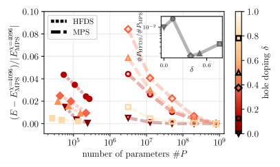
Figure 2: Comparison of energies obtained from the HFDS (filled markers, dotted lines) and MPS (empty markers, dashed lines) for a $8\times 8$ lattice at exemplary dopings $\delta$ indicated by the colorbar. For the HFDS (MPS), the number of parameters #$P_{\mathrm{HFDS}}$ (#$P_{\mathrm{MPS}}$) is varied by the number of hidden fermions $N_{h}$ (bond dimension $\chi$). For the HFDS, errorbars denoting the error of the mean are smaller than the markers. For error estimates of the MPS results see SM B. Inset: For each $\delta$, the number of parameters #$P_{\mathrm{HFDS}}(\delta)\propto N_{h}$ for the highest considered $N_{h}$ is compared to the #$P_{\mathrm{MPS}}$ needed to obtain the same energy. The fraction #$P_{\mathrm{HFDS}}/$#$P_{\mathrm{MPS}}$ indicates the efficiency of the HFDS representation. The HFDS results are obtained without enforcing the spin flip symmetry discussed in the main text.

Comparison with MPS.– The energies for the $t-J$ model are shown in Fig. 1b in green (orange, blue) for $8\times 8$ ($6\times 10$, $6\times 6$) lattices at different hole dopings $\delta$. All calculations are done for $t/J=3.0$ and open boundaries. Note that, in contrast to MPS, HFDS can be used with both open, cylindrical and periodic boundary conditions in both directions without any difference in computational cost. The open boundaries are hence mainly chosen for comparison with MPS. We compare the results from the HFDS represented by the circles using a FFNN with a single hidden layer with $128$ ($128$, $78$) nodes and $20$ hidden fermions to $SU(2)$ symmetric matrix product calculations with bond dimensions $\chi=128,\dots,2048$, corresponding to up to $\approx 6000$ $U(1)$ states, which are represented by the shaded regions. In all cases, the results from HFDS and the MPS calculations with the highest bond dimension agree very well, with even lower energies for the HFDS in the intermediate doping regime (see inset).

Note that for intermediate dopings, the MPS energies for the large system strongly change between $\chi=128,\dots,2048$ (shown by the shaded region), indicating that in this highly complicated regime with different competing energy scales $t$ and $J$ these bond dimensions are not sufficient to ensure convergence. In this regime, the power of HFDS states unfolds, as shown in more detail for $8\times 8$ systems at exemplary $\delta$ in Fig. 2: On the right side of Fig. 2, the energy over the number of parameters used by the MPS is shown, estimated as #$P_{\mathrm{MPS}}=3\chi^{2}L_{x}L_{y}$. At low and high doping, the MPS calculations converge for $\chi>512$ $SU(2)$ states, but for intermediate doping the energy significantly decreases up to the highest bond dimension $\chi=2048$ used here. Since the number of HFDS parameters #$P_{\mathrm{HFDS}}$ that can be accessed with available graphics processing units (GPU) resources is much lower than for central processing units (CPUs) used for the MPS calculations, #$P_{\mathrm{MPS}}$, we argue that for the present comparison these bond dimensions are nevertheless sufficient. For the HFDS we choose to vary #$P_{\mathrm{HFDS}}(\delta)\propto N_{h}^{2}$ at a fixed doping $\delta$ by changing the number of hidden fermions $N_{h}$. In all cases, the energies obtained with the HFDS (see Fig. 2 left) agree well with the MPS energies, but require more than two orders of magnitude less parameters.

Focusing on the highest considered #$P_{\mathrm{HFDS}}$ for each $\delta$, we calculate the #$P_{\mathrm{MPS}}$ that is needed to obtain the same energy by fitting the MPS energies to a logarithmic dependence and determining the intersection of the fit with a horizontal line through the HFDS energies. The fraction #$P_{\mathrm{HFDS}}/$#$P_{\mathrm{MPS}}$ is shown in the inset. Furthermore, the training of the HFDS on $H100$ GPUs with $1800$ steps took $6-15$ GPU hours, while the MPS calculations ran several days on a CPU. Again, it can be seen that the HFDS are particularly efficient in the intermediate doping regime.

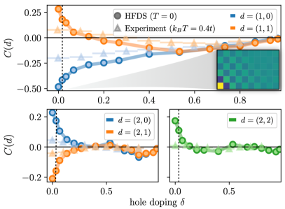
Figure 3: Two-point spin-spin correlators $C(\mathbf{d})$ for different distances $\mathbf{d}$ in the $6\times 10$ lattice. Circles represent data obtained from the optimized NQS wavefunction, triangles represent experimental data from Ref. Koepsell et al. (2021). Inset: Full spin correlation map for two holes and a reference spin in the lower left corner, colorbar limits are $-0.25$ (blue) to $0.25$ (yellow). Errorbars denoting the error of the mean are smaller than the markers.

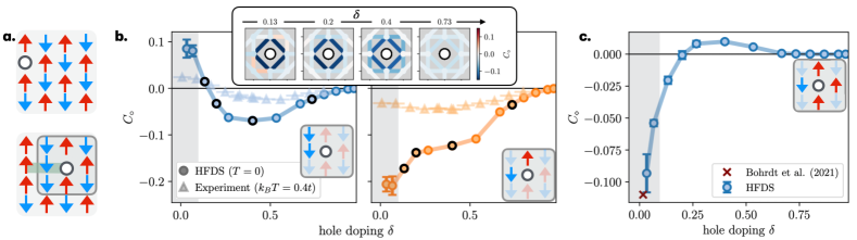
Figure 4: Investigating the polaron regime. a. Geometric string theory: When the hole (represented by the circle) moves away from its original position (top), it distorts the magnetic background (blue and red arrows), giving rise to a energy cost that increases linearly with the distance; a string (green) of length $l_{\Sigma}$. b. Three-point polaron correlators $C_{\circ}(\mathbf{d},\mathbf{r}_{h})$ for $6\times 10$ systems and different distances $\mathbf{d}$. Circles represent data obtained from the optimized NQS wavefunction, triangles the experimental data from Ref. Koepsell et al. (2021). Black markers indicate the doping values for which the full correlation map is shown in the inset. Grey areas mark the regime where errorbars are enhanced due to the occurrence of $\langle\hat{n}^{h}_{\mathbf{r}_{h}}\rangle=0$, see main text. The position of the hole relative to the spins $\mathbf{r}_{h}$ is shown in the insets. c. Five-point polaron correlations $C_{\diamond}$ for $6\times 10$ systems, with spin and hole positions as shown in the inset. For a single hole, we compare to the result from Ref. Bohrdt et al. (2021a). Errorbars (mostly smaller than the markers) show the error of the mean. In the very low doping regime marked by the gray region, positions with $\langle\hat{n}_{\mathbf{r}}\rangle=0$ exist, leading to effectively larger errors of both $C_{\circ}$ and $C_{\diamond}$. These errors are estimated by two different realizations of the HFDS, see main text.

Full doping scans.– In order to investigate the evolution of the interplay between magnetic and kinetic degrees of freedom with doping, e.g. the extent of the polaron regime, full doping scans of low energy state physical observables like correlation functions are needed. However, while at finite temperature, spin and polaron correlation functions have been measured e.g. on quantum simulation platforms realizing the Hubbard model Koepsell et al. (2021); Cheuk et al. (2016), accessing low energy or ground state observables in the full doping regime experimentally or theoretically has remained challenging. With the efficiency of the HFDS ansatz in the intermediate doping regime, such doping scans become feasible. In the following, we compare our low energy two-point spin and three-point polaron correlations to experimental measurements at finite temperature and make predictions for experimentally feasible five-point polaron correlations. In all cases, we take averages over the full system, excluding terms at the boundaries where the expectation values would involve sites outside the samples.

We start by analyzing the connected two-point spin-spin correlation function between spins at sites $\bm{r}_{1}$ and $\bm{r}_{2}$,

$$C(\mathbf{d})=\frac{1}{N_{d}}\sum_{\begin{subarray}{c}\mathbf{r}_{1},\mathbf{r}_{2}\,\mathrm{s.t.}\\ \mathbf{r}_{1}-\mathbf{r}_{2}=\mathbf{d}\end{subarray}}\eta_{\mathbf{r}_{1}\mathbf{r}_{2}}\langle\hat{S}^{z}_{\mathbf{r}_{1}}\hat{S}^{z}_{\mathbf{r}_{2}}\rangle_{c},$$ (3)

where $N_{d}$ is the number of terms in the sum, $\eta_{\mathbf{r}_{1}\mathbf{r}_{2}}=\left[\sigma(\hat{S}^{z}_{\mathbf{r}_{1}})\sigma(\hat{S}^{z}_{\mathbf{r}_{2}})\right]^{-1}$ a normalization accounting for the increased presence of holes at higher doping levels and $\langle\dots\rangle_{c}$ denotes the connected correlator with lower-order terms subtracted, as defined in SM A.2. The results for different values of $d$ are displayed in Fig. 3, and compared to experimental measurements from Ref. Koepsell et al. (2021), taken at temperature $k_{B}T=0.4t$ in the Fermi Hubbard model. Similar measurements were also taken in Ref. Cheuk et al. (2016). Although we do not expect that the finite $T$ measurements and the HFDS low energy results agree, their overall evolution upon doping agrees well: At half-filling, $d=(1,0)$ reveals a clear antiferromagnetic alignment of spins, while we observe ferromagnetic correlations at $d=(1,1)$. Upon doping, both correlations become weaker. We see the same behavior for spins at larger distances $d=(2,0),(2,1),(2,2)$, consistent with AFM Néel order at half-filling, which quickly decreases with higher doping.

At doping of $\delta\approx 0.25$, some correlations undergo a sign change. This can be understood in terms of the geometric string theory Béran et al. (1996); Grusdt et al. (2018); Bohrdt et al. (2021b), where motion of a single dopant in a magnetic background creates a string $\Sigma$ of displaced spins, see Fig. 4a. Beyond a single dopant, this description is still valid in the low doping regime Chiu et al. (2019), but with an increasing number of dopants, strings start to mix – and hence also the corresponding correlations. Once a certain level of mixing is reached, this introduces a sign change in some correlations.

Note that the full correlation map does not show any signature of a stripe phase in the low doping regime, see inset of Fig. 3, as e.g. discussed in Refs. White and Scalapino (1997, 1999); Jiang et al. (2021). This is different for cylindrical boundaries, see SM A.3.

The extent of the magnetic polaron regime can be studied in more detail by considering three-point correlations of two spins around a hole, see also Ref. Bohrdt et al. (2021b),

$$C_{\circ}(\mathbf{d},\mathbf{r}_{h})=\frac{1}{N_{d}N_{r_{h}}}\sum_{\mathbf{r}_{h}}\sum_{\begin{subarray}{c}\mathbf{r}_{1},\mathbf{r}_{2}\,\mathrm{s.t.}\\ \,\mathbf{r}_{1}-\mathbf{r}_{2}=\mathbf{d}\end{subarray}}\tilde{\eta}_{\mathbf{r}_{1}\mathbf{r}_{2}\mathbf{r}_{h}}\langle\hat{S}^{z}_{\mathbf{r}_{1}}\hat{S}^{z}_{\mathbf{r}_{2}}\hat{n}^{h}_{\mathbf{r}_{h}}\rangle_{c},$$ (4)

with the hole density $\hat{n}^{h}_{\mathbf{r}_{h}}$ and $\tilde{\eta}_{\mathbf{r}_{1}\mathbf{r}_{2}\mathbf{r}_{h}}=\left[\langle\hat{n}^{h}_{\mathbf{r}_{h}}\rangle\sigma(\hat{S}^{z}_{\mathbf{r}_{1}})\sigma(\hat{S}^{z}_{\mathbf{r}_{2}})\right]^{-1}$, measuring the influence of the hole on the spin correlations in its vicinity. The results from HFDS and experiment Koepsell et al. (2021) is shown in Fig. 4b, where the position of the $\bm{r}_{h}$ is chosen relative to the spins as sketched in the insets. For low doping, the antiferromagnetic background is perturbed by the hole as schematically illustrated in Fig. 4a, i.e. nearest neighbor ($d=(1,0)$) spins align more ferromagnetically, and diagonal neighbors ($d=(1,1)$ more antiferromagnetically. At low doping, the absolute strength of magnetic correlations decreases due to the presence of holes as observed before. Note that (4) is not well defined if $\langle\hat{n}^{h}_{\mathbf{r}_{h}}\rangle=0$. In these cases, we set the contribution of the respective term to the sum to zero. For the very low hole dopings where this problem occurs (marked by the gray area), we encounter higher errorbars, estimated by the results from two different parameterizations of the state.

Furthermore, again a sign change in the correlations with $d=(1,0)$ occurs, indicating a transition from the strongly correlated state described by magnetic string theory, to a Fermi Liquid, where the Pauli exclusion principle leads to enhanced antiferromagnetic alignment Hartke et al. (2020). For cuprate materials, the same qualitative change of observables takes place at a similar doping level Keimer et al. (2015). Note that the presence of real space pairs would lead to similar signatures as observed here for the polaron correlations White and Scalapino (1997).

To further investigate the nature of the polaron, the five-point correlator

$$C_{\diamond}=\frac{2^{4}}{N_{r}}\sum_{\mathbf{r}_{h}}\frac{1}{\langle\hat{n}^{h}_{\mathbf{r_{h}}}\rangle}\langle\hat{n}^{h}_{\mathbf{r_{h}}}\hat{S}^{z}_{\mathbf{r_{h}}+\hat{e}_{x}}\hat{S}^{z}_{\mathbf{r_{h}}-\hat{e}_{x}}\hat{S}^{z}_{\mathbf{r_{h}}+\hat{e}_{y}}\hat{S}^{z}_{\mathbf{r_{h}}-\hat{e}_{y}}\rangle$$ (5)

is considered Bohrdt et al. (2021a) in Fig. 4c. At very low doping, $C_{\diamond}$ depends on the probability of configurations with string lengths $l_{\Sigma}=0$ and $l_{\Sigma}>0$. As schematically shown in Fig. 4a, $C_{\diamond}>0$ for $l_{\Sigma}=0$, while for $l_{\Sigma}>0$, $C_{\diamond}<0$. The fact that we find $C_{\diamond}<0$ indicates that configurations with $l_{\Sigma}>0$ are more likely, in agreement with Ref. Grusdt et al. (2019).

Conclusion.– In this work, we demonstrate that hidden fermion determinant states (HFDS) effectively capture the low-energy states of the $t-J$ model. Particularly, we show that HFDS can encode energies comparable to those obtained from matrix product state (MPS) calculations with $2048$ $SU(2)$ symmetric states across the full doping regime, while utilizing up to four orders of magnitude fewer parameters. This parameter efficiency positions HFDS as a competitive alternative to MPS, particularly as GPU resources continue to advance.

In addition to improving training speed, reducing parameter count makes it easier to save model weights as they take up far less memory. As a result, we are able to share model weights across the full doping scan so that others can access the trained models. The model weights can either be used to compute new correlation functions, or as a starting point for simulating closely related models.

Our analysis reveals that HFDS excel in the intermediate doping regime, facilitating the exploration of low-energy observables throughout the entire doping scan. Specifically, we investigate spin and polaron correlations, comparing our findings with experimental data. The doping dependence of these correlation functions, and the critical dopings at which their signs change, aligns well with existing literature. This work paves the way for further investigations of correlated systems across the full doping range and low temperatures.

Code availability. Our implementation of hidden fermions is adapted from the neural backflow https://netket.readthedocs.io/en/latest/tutorials/lattice-fermions.html and is available at https://github.com/HannahLange/HFDSfortJ, where also the trained models can be found.

Acknowledgements. We thank Fabian Grusdt and Tizian Blatz for useful discussions. All DMRG calculations were performed using the SyTeN toolkit developed and maintained by C. Hubig, F. Lachenmaier, N.-O. Linden, T. Reinhard, L. Stenzel, A. Swoboda, M. Grundner, S. Mardazad, F. Pauw, and S. Paeckel. Information is available at https://syten.eu and in SM B. A. Bohrdt, A. Böhler and H. Lange acknowledge the support by the Deutsche Forschungsgemeinschaft (DFG, German Research Foundation) under Germany’s Excellence Strategy—EXC-2111—390814868. H. Lange acknowledges support by the International Max Planck Research School for Quantum Science and Technology (IMPRS-QST).
C. Roth acknowledges support from the Flatiron Institute. The Flatiron Institute is a division of the Simons Foundation.

Supplemental Material

Appendix A Definitions and Additional Results

A.1 Convergence for the $6\times 10$ systems

Below, we show the same convergence analysis as in Fig. 2 for the $6\times 10$ systems.

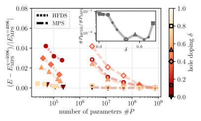
Figure 5: Comparison of energies obtained from the HFDS (filled markers, dotted lines) and MPS (empty markers, dashed lines) for a $6\times 10$ lattice at exemplary dopings $\delta$ indicated by the colorbar. For the HFDS (MPS), the number of parameters #$P_{\mathrm{HFDS}}$ (#$P_{\mathrm{MPS}}$) is varied by the number of hidden fermions $N_{h}$ (bond dimension $\chi$). For the HFDS, errorbars denoting the error of the mean are smaller than the markers. Inset: For each $\delta$, the number of parameters #$P_{\mathrm{HFDS}}(\delta)\propto N_{h}$ for the highest considered $N_{h}$ is compared to the #$P_{\mathrm{MPS}}$ needed to obtain the same energy. The fraction #$P_{\mathrm{HFDS}}/$#$P_{\mathrm{MPS}}$ indicates the efficiency of the HFDS representation. The HFDS results are obtained without enforcing the spin flip symmetry discussed in the main text.

A.2 Definition of the connected correlation functions

The two-point spin-spin correlations (3), as well as the three-point polaron correlations (4) shown in the main text are defined as the connected versions. When writing out the connected correlators $\langle\dots\rangle_{c}$ used in the main text, they take the following forms:

• The two-point spin-spin correlations (3) are

  $$C(\mathbf{d})=\frac{1}{N_{d}}\sum_{\mathbf{r}_{1},\mathbf{r}_{2}\,\mathrm{s.t.}\,\mathbf{r}_{1}-\mathbf{r}_{2}=\mathbf{d}}\eta_{\mathbf{r}_{1}\mathbf{r}_{2}}\left(\langle\hat{S}^{z}_{\mathbf{r}_{1}}\hat{S}^{z}_{\mathbf{r}_{2}}\rangle-\langle\hat{S}^{z}_{\mathbf{r}_{1}}\rangle\langle\hat{S}^{z}_{\mathbf{r}_{2}}\rangle\right)$$ (6)

• The three-point polaron correlations (4) are

  $$C_{\circ}(\mathbf{d},\mathbf{r}_{h})=\frac{1}{N_{d}N_{r_{h}}}\sum_{\mathbf{r}_{h}}\sum_{\mathbf{r}_{1},\mathbf{r}_{2}\,\mathrm{s.t.}\,\mathbf{r}_{1}-\mathbf{r}_{2}=\mathbf{d}}\tilde{\eta}_{\mathbf{r}_{1}\mathbf{r}_{2}\mathbf{r}_{h}}\Big{(} \langle\hat{S}^{z}_{\mathbf{r}_{1}}\hat{S}^{z}_{\mathbf{r}_{2}}\hat{n}_{\mathbf{r}_{h}}\rangle-\langle\hat{S}^{z}_{\mathbf{r}_{1}}\rangle\langle\hat{S}^{z}_{\mathbf{r}_{2}}\hat{n}_{\mathbf{r}_{h}}\rangle-\langle\hat{S}^{z}_{\mathbf{r}_{1}}\hat{S}^{z}_{\mathbf{r}_{2}}\rangle\langle\hat{n}_{\mathbf{r}_{h}}\rangle$$

  $$-\langle\hat{S}^{z}_{\mathbf{r}_{2}}\rangle\langle\hat{S}^{z}_{\mathbf{r}_{1}}\hat{n}_{\mathbf{r}_{h}}\rangle+2\langle\hat{S}^{z}_{\mathbf{r}_{1}}\rangle\langle\hat{S}^{z}_{\mathbf{r}_{2}}\rangle\langle\hat{n}_{\mathbf{r}_{h}}\rangle\Big{)}$$ (7)

A.3 Discussion of the stripe phase

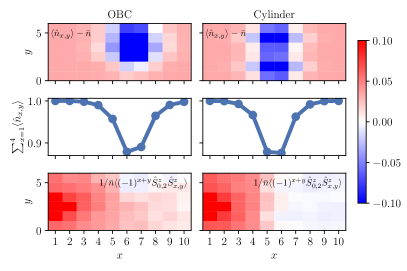
Figure 6: Open and cylindrical boundaries: We show the local density $\langle\hat{n}_{x,y}\rangle-\bar{n}$ with $\bar{n}=1-\delta$ (top), the average rung density (middle) and the staggered and normalized spin correlations $1/\bar{n}\langle(-1)^{x+y}\hat{S}^{z}_{0,2}\hat{S}^{z}_{x,y}\rangle$ for systems with hole doping $\delta=0.03$ ($N=58$, left) and $\delta=0.80$ ($N=12$, right), comparing open (left column) and cylindrical (i.e. open in the long direction, periodic in the short direction, right column) boundaries.

Below, we show that while there are no clear signatures for stripes for the open boundary systems considered in the main text, cylindrical boundaries (i.e. open in the long $x$ direction, periodic in the short $y$ direction) can give rise to stripe signals in the density and spin correlations.

In Fig. 6 we show the local density $\langle\hat{n}_{x,y}\rangle-\bar{n}$, subtracted by the average filling $\bar{n}=1-\delta$ as well as the average rung density for both boundary conditions and exemplary hole doping $\delta=0.03$ ($N=58$, left) and $\delta=0.80$ ($N=12$, right) in the top two rows. For both boundary conditions, we find a modulation of the density in the $y$ direction, with slightly more pronounced peaks for the cylindrical boundaries at $\delta=0.80$. Furthermore, we calculate the staggered and normalized spin correlations

$$\frac{1}{\bar{n}}\langle(-1)^{x+y}\hat{S}^{z}_{0,2}\hat{S}^{z}_{x,y}\rangle.$$

For the cylindrical boundaries, we find that the signal of these correlations is suppressed when $x,y$ are behind a density modulation with filling lower than the average, most prominently for $\delta=0.03$, indicating a stripe-like phase.

A.4 Hole-hole correlations

Fig. 7 shows the hole-hole correlations

$$g^{2}(\mathbf{d})=\sum_{\mathbf{r}_{i},\,\mathbf{r}_{j},\mathrm{s.t.}\,\mathbf{r}_{i},\mathbf{r}_{j}=\mathbf{d}}\left(\langle\hat{n}_{\mathbf{r}_{i}}\hat{n}_{\mathbf{r}_{j}}\rangle/(\langle\hat{n}_{\mathbf{r}_{i}}\rangle\langle\hat{n}_{\mathbf{r}_{j}}\rangle)\right)-1$$ (8)

across the full doping range. In all cases, the observed hole-hole correlations are negative i.e. we do not observe any signatures of hole bunching, which in principle could arise from interactions between the holes mediated by the spin background. This is in agreement with the experimental data from Ref. Koepsell et al. (2021) (see triangles), that was available for $\mathbf{d}=(1,0)$ and $\mathbf{d}=(1,1)$ (see left panel).

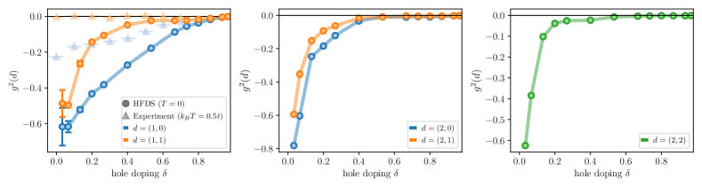
Figure 7: Hole-hole correlations $g^{2}(\mathbf{d})$ as defined in Eq. (8) for different distances $\mathbf{d}=(1,0),(1,1)$ (left), $\mathbf{d}=(2,0),(2,1)$ (middle) and $\mathbf{d}=(2,2)$ (right). For $\mathbf{d}=(1,0),(1,1)$ the results are compared to experimental measurements from Ref. Koepsell et al. (2021).

Appendix B Density Matrix Renormalization Group Benchmarks

The benchmarks using matrix product states (MPS) shown in this work were obtained using the density matrix renormalization group (DMRG) algorithm Schollwöck (2011). Specifically, we use the the SyTen toolkit Hubig et al. ; Hubig (2017) with implemented global $U(1)_{N}$ and $SU(2)$ symmetries and bond dimensions up to $\chi=2048$ (corresponding to $\approx 12000$ $U(1)$ states). We use the single-site (DMRG3S) in all stages except for the last stage, we the two-site (2DMRG) update scheme is applied. In total, $5$ stages with $40$ sweeps in the first two stages, $20$ sweeps in the intermediate stage and $10$ sweeps in the final stage were used.

As discussed in the main text, we do not expect that our MPS are fully converged in the intermediate doping regime. In order to estimate the MPS error, we follow Ref. Corboz (2016) and calculate the truncation error per site $\epsilon_{\mathrm{Trunc}}$ at each bond dimension. Then, we fit the MPS energies $E_{\mathrm{MPS}}^{\chi}$ with a linear dependence on the truncation error, as shown in Fig. 8 on the right. The lines on the right plot show the respective fits $E_{\mathrm{fit}}(\epsilon_{\mathrm{Trunc}})$ for exemplary doping values $\delta$ (the same as shown in Fig. 2). The error is estimated as

$$\Delta=\left[(E_{\mathrm{MPS}}^{\chi=2048}-E_{\mathrm{fit}}(\epsilon_{\mathrm{Trunc}}=0)\right]/2$$ (9)

and shown on the left of Fig. 8. We find a particularly high error for $\delta=0.4$.

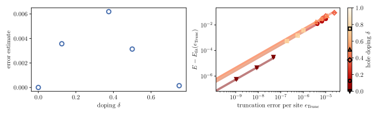
Figure 8: Estimation of MPS errors for the $8\times 8$ systems. Left: The estimated errors on the MPS energies $E_{\mathrm{MPS}}^{\chi}$ obtained with bond dimension $\chi=2048$ and $SU(2)$ symmetry. The error estimates are obtained by fitting the MPS energies $E_{\mathrm{MPS}}^{\chi}$ w.r.t. the truncation error per site, $\epsilon_{\mathrm{Trunc}}$. Hereby, the two lowest bond dimensions were neglected. The lines on the right plot show these fits $E_{\mathrm{fit}}(\epsilon_{\mathrm{Trunc}})$. The error is estimated as $\left[(E_{\mathrm{MPS}}^{\chi=2048}-E_{\mathrm{fit}}(\epsilon_{\mathrm{Trunc}}=0)\right]/2$ Corboz (2016).

Appendix C The Hidden Fermion Determinant States

C.1 Comparison to Moreno et al. – the Fermi Hubbard model

As a first benchmark, we compare the results obtained with our HFDS implementation with results from Moreno et al. Moreno et al. (2022) for the Fermi Hubbard model on a $4\times 4$ lattice with periodic boundary conditions. In contrast to this work, we use a single FFNN network for all entries of the lower block of the Slater determinant shown in Fig. 1a. This differs slightly from the HFDS used in Moreno et al. Moreno et al. (2022), where multiple networks for each row of the lower block were employed. In Fig. 9, we compare the relative energies obtained with both HFDS variants for $N=8$ fermions on a $4\times 4$ lattice (blue lines). In both cases, we use $8$ hidden fermions and $128$ features. The results agree within the errorbars, although the number of parameters #$P$ is smaller for the single network. Furthermore, we compare our results (blue) with results from Moreno et al. Moreno et al. (2022) (orange) that were obtained with similar #$P$. Again, we find a good agreement.

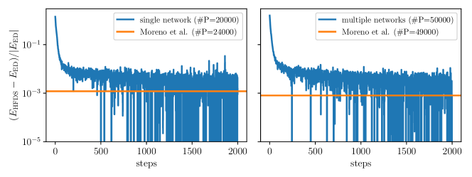
Figure 9: Results for the Fermi Hubbard model on a $4\times 4$ lattice with $N=8$ fermions and periodic boundary conditions. We use a single FFNN network for all entries of the lower block of the Slater determinant (left). This is slightly different to the HFDS used in Moreno et al. Moreno et al. (2022), where multiple networks for each row of the lower block were employed (right). Hence, the number of parameters #$P$ differs. We compare our results (blue) with results from Moreno et al. Moreno et al. (2022) (orange) that were obtained with similar #$P$. In all cases, $8$ hidden fermions were used.

C.2 Backflow vs. Hidden fermions

We compare the HFDS to the neural backflow architecture for a system of $L_{x}\times L_{y}=4\times 4$ lattice sites, where we choose the size of the corresponding networks such that they have an approximately equal number of variational parameters. We use the same number of hidden and visible fermions at each doping for the HFDS and adjust the number of features of the backflow network accordingly. Both networks are parameterized by a FFNN with 3 layers and start from a random initial state. Results for the final variational energy are shown in Fig. 10. We find that both architectures lead to the same final energies across all dopings, consistent with the claim that they can be unified within the neural Jastrow-backflow framework Liu et al. (2019).

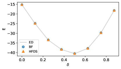
Figure 10: Results for optimized neural backflow states and HFDS. Both states are parametrized by a single FFNN and start from the same random initial state. The network sizes were chosen such that at each doping the number of parameters is approximately equal, between #$P=22000$ at $\delta=0.875$ and #$P=71000$ at $\delta=0$.

C.3 Initializations

We further compare different initial states for the mean field of visible fermions. As described in the main body, the upper left block matrix can be initialized by a physically motivated state, while the other blocks are set to zero or identity, respectively. Fig. 11 compares a Gutzwiller projected Fermi sea for both open and periodic boundary conditions to a random parameter initialization. The Fermi sea initialization is further described below, see Sec. C.3. We choose the particularly challenging low doping case $\delta=1/8$ for our benchmarks. The Fermi sea is initialized by building the mean field matrix out of the single particle eigenstates of a tight-binding Hamiltonian with either open or periodic boundary conditions. While both Fermi seas achieve similar final energies as the random initial state, we see a slight improvement in convergence time for the Fermi sea states.

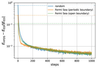
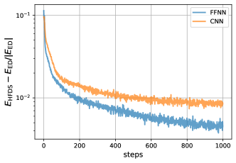
Figure 11: Optimization curves for different initial mean field states (left) and architectures (right) for $\delta=0.125$. All states were optimized with the same network with #$P=60000$ parameters. Only the initial configuration of the upper left block in the Slater determinant, and the network representing the lower half respectively, was changed. The different architectures are compared for an open boundary Fermi sea initialization. The random state optimization corresponds to the final value at $\delta=0.125$ in Fig. 10.

Fermi sea initialization

Periodic boundaries: If we initialize a Fermi sea of a periodic boundary system, the parameters of the momentum eigenstates are obtained straightforwardly by applying a Fourier transform to the real space states $|\psi_{k}\rangle=\psi_{k}(x)|x\rangle$:

$$\psi_{k}(x)=e^{ikx}\psi_{x}.$$

Note that this makes the mean field parameters complex. Hence, if the rest of the network is real, this leads to a HFDS that has both imaginary and real weights, and complicates the gradient calculation using SR. These complications can in principle be overcome, however, it is easier to circumvent this issue by a basis change: For the free electron model $E(k)=E(-k)$, so instead of building the Fermi sea out of states $|k\rangle$ and $|-k\rangle$ one can use $|k^{+}\rangle=\frac{1}{2}(|k\rangle+|-k\rangle)$ and $|k^{-}\rangle=\frac{1}{2i}(|k\rangle-|-k\rangle)$. This leads to new parameters

$$\psi_{k^{+}}(x)=\frac{1}{2}(e^{ikx}+e^{-ikx})\psi_{x}=\cos(kx)\psi_{x},$$

$$\psi_{k^{-}}(x)=\frac{1}{2i}(e^{ikx}-e^{-ikx})\psi_{x}=\sin(kx)\psi_{x},$$

which are purely real.

Open boundaries: For the open boundary systems discussed in the main text we choose a slightly different initialization by making use of an exact solution of the open boundary single particle tight-binding model,

$$\hat{H}=\sum_{i,j}\left(\hat{c}_{i}^{\dagger}\hat{c}_{j}+\text{h.c.}\right).$$

Diagonalization gives the single particle orbitals for non-interacting particles in a system with open boundaries.

C.4 Different network architectures

We further compare the optimization for different network architectures, namely a FFNN and a CNN. Fig. 11 shows the relative error of the energy compared to an exact solution. We see that the FFNN achieves slightly better variational energies than the CNN. Both networks are initialized with a projected open boundary Fermi sea.

References

- Improved energy extrapolation with infinite projected entangled-pair states applied to the two-dimensional hubbard model. Phys. Rev. B 93, pp. 045116. External Links: Document, Link Cited by: Figure 8, Appendix B.
- [2] The SyTen toolkit.. Note: https://syten.eu Cited by: Appendix B.
- Symmetry-protected tensor networks. LMU München. Note: https://edoc.ub.uni-muenchen.de/21348/ Cited by: Appendix B.
- Microscopic evolution of doped mott insulators from polaronic metal to fermi liquid. Science 374 (6563), pp. 82–86. External Links: Document, https://www.science.org/doi/pdf/10.1126/science.abe7165, Link Cited by: Figure 7, §A.4.
- Machine learning by unitary tensor network of hierarchical tree structure. New Journal of Physics 21 (7), pp. 073059. External Links: Document, Link Cited by: §C.2.
- Fermionic wave functions from neural-network constrained hidden states. Proceedings of the National Academy of Sciences 119 (32), pp. e2122059119. External Links: Document, https://www.pnas.org/doi/pdf/10.1073/pnas.2122059119, Link Cited by: Figure 9, §C.1.
- The density-matrix renormalization group in the age of matrix product states. Annals of Physics 326 (1), pp. 96–192. Note: January 2011 Special Issue External Links: ISSN 0003-4916, Document, Link Cited by: Appendix B.