Superconnections in AdS/QCD and
the hadronic light-by-light contribution to the muon
Abstract
In this paper, we consider hard-wall AdS/QCD models extended by a string-theory inspired Chern-Simons action in terms of a superconnection involving a bi-fundamental scalar field which corresponds to the open-string tachyon of brane-antibrane configurations and which is naturally identified with the holographic dual of the quark condensate in chiral symmetry breaking. This realizes both the axial and chiral anomalies of QCD with a Witten-Veneziano mechanism for the mass in addition to current quark masses, but somewhat differently than in the Katz-Schwartz AdS/QCD model used previously by us to evaluate pseudoscalar and axial vector transition form factors and their contribution to the HLBL piece of the muon . Compared to the Katz-Schwartz model, we obtain a significantly more realistic description of axial-vector mesons with regard to - mixing and equivalent photon rates. Moreover, predictions of the branching ratios are found to be in line with a recent phenomenological study. However, pseudoscalar transition form factors compare less well with experiment; in particular the transition form factor turns out to be overestimated at moderate non-zero virtuality. For the combined HLBL contribution to the muon from the towers of axial vector mesons and excited pseudoscalars we obtain, however, a result very close to that of the Katz-Schwartz model.
I Introduction
The anomalous magnetic moment of the muon has been measured to date with a world-average error of 0.19 ppm [1, 2], corresponding to a standard deviation of in , and this uncertainty is expected to be further reduced by about a factor of 2 with the final result of the current experiment at Fermilab by the Muon Collaboration. The Standard Model prediction of is limited by uncertainties in the contribution from hadronic vacuum polarization (HVP), where data-driven and lattice calculations aim at per-mille accuracy to match the experimental precision, but currently deviate from each other beyond their respective error estimates [3]. Once this discrepancy is resolved, the uncertainty of the much smaller hadronic light-by-light (HLBL) scattering contribution will be again of comparable importance as it contributes an error of according to the 2020 White Paper of the Muon Theory Initiative [4]. This uncertainty is dominated by the effect of short-distance constraints (SDCs) [5, 6, 7, 8, 9, 10, 11, 12, 13, 14] and axial vector contributions, for which errors of and , respectively, have been estimated in [4], corresponding to 67 and 100 % of the assumed values.111The 100% uncertainty in the axial-vector contribution is due to the fact that conventional hadronic models [5, 15, 16, 17, 18, 19] disagree even in the order of magnitude, with some of them yielding contributions above , some less than .
In hadronic models, SDCs can typically only be satisfied by infinite towers of resonances. The estimate of their effects in [4] was based on a Regge model of excited pseudoscalars subjected to available experimental constraints [9, 8], although in the chiral limit excited pseudoscalars decouple from the axial anomaly responsible for the longitudinal Melnikov-Vainshein SDC; the alternative of excited axial vector mesons was not considered because of technical difficulties and sparse experimental data. However, in [20, 21] it was shown that in chiral bottom-up holographic QCD (hQCD) models the longitudinal SDC is naturally satisfied by the infinite tower of axial-vector mesons. Remarkably, the short-distance behavior of their transition form factors (TFFs) obtained in [20] agrees exactly with the recently derived asymptotic behavior in a light-cone expansion [22] in analogy to the Brodsky-Lepage limit of the TFF of pseudoscalars, for which such an agreement was noted already in [23]. In the case of the individual TFFs, it is the infinite tower of vector resonances of holographic models which is responsible for this feature, while for the complete HLBL four-point function, the infinite tower of axial vector mesons is required for satisfying the longitudinal SDC. While the simplest chiral hQCD models involve only Goldstone bosons and no excited pseudoscalars, also in the slightly more complicated models that admit massive pions, it was found that the longitudinal SDC is saturated by the tower of axial vector mesons as opposed to the tower of excited pseudoscalars [24].
In [25] we have employed the model of Katz and Schwartz (KS) [26, 27, 28], where in addition to quark masses the effects of the U(1)A anomaly are incorporated, to extend the numerical predictions of flavor-symmetric hard-wall hQCD models to the contributions of the heavier mesons (with a pseudoscalar glueball mixing in) and axial vector mesons together with their radial excitations. By including a gluon condensate as one further parameter and accounting for gluonic corrections to the asymptotic behavior of TFFs, we have found that the masses of all pseudo-Goldstone bosons as well as their two-photon couplings can be reproduced at the percent level, yielding contributions in complete agreement with the WP2020 estimate. In this particular hQCD model, the contributions from the axial-vector and excited pseudoscalar towers amounted to and , respectively, somewhat reducing the previous flavor-symmetric hard-wall result , to be compared with the WP2020 estimate of for axial-vector plus SDC contributions.
However, while the octet-singlet mixing in the pseudoscalar sector and the resulting photon couplings predicted by the KS model are very close to experimental data, the predicted mixing of and axial vector mesons is rather far from experimental findings, pointing to the need of further refinements. Adopting some parts of the construction of improved hQCD models in [29, 30], in this paper we consider a simple hard-wall hQCD model where both flavor and axial anomalies are implemented by a Chern-Simons action that follows more closely a string-theoretic setup with brane-antibrane configurations. Besides a somewhat different implementation of the U(1)A anomaly than in the KS model, this leads to a Chern-Simons action involving the bi-fundamental scalar field corresponding to the open-string tachyon responsible for brane-antibrane merging and thus chiral symmetry breaking. Remarkably, this yields a significantly more realistic description of - mixing, the equivalent photon rates, and the slope parameters of axial-vector TFFs, but at the price of pseudoscalar transition form factors that now overestimate experimental data at non-zero photon virtualities. The resulting HLBL contributions to are found to be smaller for the axial vector mesons and larger for the pseudoscalars, with rather little changes in the sum total. While not yet a completely satisfying hQCD model, we consider these results as encouraging with regard to the potential of more elaborate string-inspired hQCD models along the lines of Refs. [29, 30] and also as providing an idea of the range of systematic errors of current hQCD results for the HLBL contribution to the muon .
This paper is organized as follows. In Sec. 2 we give a brief introduction to the tachyon condensation models of [29, 30] which are inspired by brane-antibrane constructions in string theory. In Sec. 3 we describe explicitly the HW AdS/QCD model with relevant parts of the scalar-extended Chern-Simons term included, before detailing the equations of motion and the normalizations for its solutions for both pseudoscalar and axial vector resonances in Sec. 4. In Sec. 5 and 6, we discuss and evaluate the resulting TFFs and also the decay rate of axial vector mesons in electron-positron pairs, which has been proposed in Ref. [31] as an indirect check of doubly virtual axial-vector TFFs. We also discuss briefly scalar mesons, which in the simplest HW AdS/QCD models do not participate in the HLBL scattering amplitude but for which the tachyon-condensation models suggest a specific form of photon interactions. Finally, we present numerical results for the various HLBL contributions to , comparing the different hQCD models with U(1)A anomaly.
In the appendices, we describe an important matching factor and the explicit forms appearing in the Chern-Simons term in detail, and we provide details on scalar TFFs.
II Brane anti-brane systems and superconnections
In this section we briefly review some features of - systems in the context of holography, closely following [29]. We describe some features of the resulting open-string tachyon condensation models and focus in particular on the Chern-Simons term, which we will subsequently include in a simple bottom-up hard-wall (HW) AdS/QCD model.
The string-theoretic construction is based on a configuration of branes intersecting with and branes in type IIA or type IIB string theory. In the large (’t Hooft) limit, the color branes are described by background values of the massless string fields (including the graviton), while the flavor branes (which all sit on top of each other) are treated as non-backreacting probe branes. This yields a dual gauge theory with gauge group with matter in the fundamental representation and a global symmetry group of , whose part will be broken by an anomaly. The fields localized to the flavor branes will be a gauge field and a complex scalar field in the bi-fundamental representation of the gauge group.
The low-energy effective action contains a tachyonic mass term for associated with the annihilation of and branes into lower dimensional strings and branes, which (at least in flat space) is given by , with being the fundamental string tension. In order to interpret the scalar as the dual field of the quark condensate operator , its mass has to be set to ; hence, the AdS radius has to satisfy . This of course signals a breakdown of the supergravity approximation, which will nevertheless be taken as the basis of constructing a phenomenological bottom-up model for QCD.
Holographic QCD models from tachyon condensation [32, 33](and their extensions to the Veneziano limit [34, 30]) are obtained by prescribing an AdS-like background, setting and ignoring all higher string theory modes (or including their effects in various different effective potentials). They are semiclassically self-consistent, and the scalar obtains a stable background value (i.e. condenses), which describes chiral symmetry breaking in the boundary theory.
These models contain a particularly interesting generalization of the usual Chern-Simons term that involves a superconnection.222This generalization has been recently shown to be the appropriate framework for a wider class of anomalies including also systems with interfaces and spacetime boundaries [35, 36]. The world-volume action of the flavor and anti-flavor branes splits into two parts, , where the Chern-Simons part is given by
| (1) |
with
| (2) | ||||
Here is a formal sum of Ramond-Ramond (RR) -form potentials and the integral is supposed to pick the -form part of the integrand.
Contrary to the DBI action, the Chern-Simons action can be derived from boundary string field theory to all orders in [37, 38]. The above structure actually has a very geometric origin in Quillen’s theory of superconnections on graded vector bundles [39]. is known as the curvature of the superconnection and the multiplication implicit in the definition of the exponential is a generalization of the usual matrix multiplication. A useful aspect of Quillen’s results is that when the bundle is trivial (which we will assume in the rest of the paper) is a total derivative. In the setup of [29], the color branes generate an RR flux proportional to , which gets picked up by the 5 form part . After effectively reducing dimensionally to , there is a quadratic coupling of the RR potential and the fields contained in ; this is responsible for the correct implementation of the anomaly. Hence, the two most important terms from the Chern-Simons action will be
| (3) |
In the following section we implement this structure into a hard-wall (HW) hQCD model. While the first term is subleading in , it plays an important role phenomenologically, as it will be responsible for the large mass of the meson.
III Hard-wall AdS/QCD model with scalar-extended Chern-Simons term
Upon expanding the DBI action of the tachyon condensation models, one obtains in lowest order of exactly the action of the original HW AdS/QCD models of Ref. [40, 41] which are known to be well suited for the description of low lying mesons. The tachyon can be identified with the bi-fundamental scalar of the HW models. There is, however, an important factor that determines the interactions in the Chern-Simons term involving the scalar fields. The relation, which is derived in Appendix A, is
| (4) |
where is the 5-dimensional Yang-Mills coupling of flavor gauge fields and is a bi-fundamental scalar field dual to bilinear quark operators. Since the tachyon has dimension 1 and has mass dimension , we obtain the correct mass dimension for , namely .
In bottom-up HW models, the background geometry is simply pure , which (upon setting the AdS radius equal to 1) has a metric
| (5) |
in Poincaré coordinates. Confinement and conformal symmetry breaking is implemented by a sharp cutoff at , where one has to specify boundary conditions for the fields.
The complete action relevant to the processes that we will consider later reads
| (6) |
where it is understood that we replace by and any occurrence of in the Chern-Simons terms has to be replaced by (4). The first three integrals are identical to the usual HW action upon setting in .
In the AdS geometry, the scalar field admits a background of the form
| (7) |
where the matrices are proportional to the quark masses and the chiral condensate in the dual theory. We will restrict to , with but uniform . These parameters together with will be fitted to , and OPE data below.
The fluctuations around the vacuum of the scalar and the longitudinal gauge fields describe scalar and pseudoscalar mesons, while the transverse degrees of freedom of the gauge fields describe vector and axial-vector mesons. We parametrize the pseudoscalar fluctuations of as [42]
| (8) |
where .
In (III) we have included a phenomenological background field in the kinetic term of the RR 3-form, which will eventually account for the running of the QCD coupling in the gluon condensate. Some explicit expressions for relevant for our discussion are given in a separate appendix. It is possible to dualize the last line of (III) to
| (9) |
where can be interpreted as a pure pseudoscalar glueball field (before its eventual mixing with pseudoscalar mesons). Note that is only defined up to an extra closed term with integer periods . These are exactly the gauge symmetries of a circle-valued scalar, so this action is well-defined. As is shown in the appendix, to leading order in pseudoscalar fluctuations,
| (10) |
Upon rescaling333Since is a circle-valued scalar, this rescaling would affect the normalization of its periods. We are however not interested in situations with nonzero winding. by a factor of , one arrives at
| (11) |
with
| (12) | ||||
| (13) |
The action in terms of the components of the field can be written as
| (14) |
with . Upon expanding this action at small we find
| (15) |
This is, asymptotically, of the same form as the action of the KS model [26], with identified with
| (16) |
of [25]. As explained in that paper, a fit to the OPE of QCD forces the leading part of to be proportional to the running coupling . The subleading part is a consequence of the demanding consistency of the EOM of [25]; it allows us to include a non-zero gluon condensate, parametrized by , and we will take over this explicit form to the present model.
IV Equations of motion and meson modes
We first list the quadratic part of the action and the equations of motion for the pseudoscalar sector that follow from it. The pseudoscalar action for the subsector reads
| (17) |
where the spacetime indices are contracted with the 5d Minkowski metric and
| (18) |
Flavor traces of the tachyon potential will be written as
| (19) |
In the following we will work in the gauge. The pseudoscalar fluctuations of the gauge field are parametrized as . The equations of motion in the pseudoscalar sector for read
| (20) |
In these equations a sum over the index is understood. The last equation is the equation of motion.
The sector is not affected by the addition of , which implements the U(1)A anomaly; the corresponding fluctuation equations are the same as in [24].
An important point is the choice of boundary conditions. After varying the action, the boundary term that has to vanish at and is
| (21) |
which upon using the equation of motion reads
| (22) |
In the rest of the paper we will be choosing so-called [24] HW3 boundary conditions at , i.e. , supplemented by .
In order to compute correlation functions of operators or masses and decay constants of particles in the dual gauge theory we need to solve the set of equations (IV) subject to the above boundary conditions in the infrared. For the former, one has to supply boundary conditions in the UV which make the solution non-normalizable, while for the latter, one has to consider normalizable modes. Normalizable modes only exist for discrete values of which can be identified with the mass squared of a pseudoscalar meson. The inner product from which the norm follows reads
| (23) |
The decay constants are defined as in [25] and read
| (24) | |||
| (25) |
The equations of motion for the axial vector mesons read
| (26) |
Their norm is given by
| (27) |
and the decay constants are computed by
| (28) |
IV.1 Parameter settings
The HW AdS/QCD model with scalar-extended Chern-Simons terms thus constructed will be referred to as CS” in the following. We shall also consider a variant CS’, where the tachyon is only appearing in , which implements the U(1)A anomaly, but where involves only flavor gauge fields.444In the sector, the CS’ model is in fact identical to the HW3 model considered in [24]. These two models will be compared with the version of the KS model evaluated by us in [25], to which we refer for detailed tables of numerical results. All three models, for which we take and , have the same number of free parameters, which will be fixed by MeV, MeV,
| (29) | |||||
and a least-square fit of and .
The coupling constant is usually fixed by the OPE of the vector current correlator as
| (30) |
but we shall alternatively consider matching the decay constant of the meson, which in the HW model leads to [43]
| (31) |
The latter in fact significantly improves the holographic result for the hadronic vacuum polarization [43], and such an reduction of is also warranted by comparing with next-to-leading order QCD results for the vector correlator at moderately large values [44, 45, 13].
IV.2 Scalar mesons
Scalar mesons are naturally present in this model as scalar fluctuations of the field . With just the terms quadratic in included in (III), the spectrum will be flavor symmetric and there is no coupling to two photons for the mesons.555The string-theoretic motivation of AdS/QCD models also suggests flavor-singlet scalar and tensor mesons in the form of dilaton and metric fluctuations dual to glueball modes, which inevitably have two-photon couplings from vector-meson dominance. In the Witten-Sakai-Sugimoto model, their contributions to have been estimated [46] to be below the level of . In [47], metric fluctuations have been used as a model for tensor mesons in general (with adjusted coupling strength), even though they do not naturally form flavor multiplets.
However, if one introduces tachyon potentials also in the Yang-Mills action, as done in the improved hQCD models of Ref. [29, 48, 49, 32, 33, 34], one obtains additional terms such as
| (32) |
which after expanding break the flavor symmetry of the excitations and introduce quark mass effects to the spectrum, and
| (33) |
which leads to a nonzero TFF. We have introduced here by hand the phenomenological parameter in front of both terms, whose deviation from measures how much our model differs from the original action (III); corresponds to keeping the terms of order from (65) in the Yang-Mills action.
The mode equations for are
| (34) |
subject to boundary conditions and for small . The normalization is
| (35) |
where the sum over is understood.
The masses that are obtained for such scalars are, however, too large to be identified with the scalar mesons , , and , which are of predominant interest for the HLBL contribution. In fact, those are likely tetraquark states and thus presumably beyond a holographic description in the large- ’t Hooft limit. With and as in (30), the scalar masses are 1.722, 1.722, and 2.084 GeV; with reduced coupling (31) slightly smaller: 1.610, 1.610, and 2.006 GeV. We thus do not consider them any further here, because with these parameters they contribute negligibly to (only ). We provide, however, some additional pertinent comments on their TFFs in Appendix C.
V Transition form factors
[GeV]
[GeV2]
Using the expressions for derived in the appendix, we can obtain the transition form factors for the pseudoscalar mesons ( is the quark charge matrix)
| (36) |
where is the bulk-to-boundary vector propagator
| (37) |
for photon virtualities and the prime denotes differentiation with respect to . Partial integration yields
| (38) |
up to total derivatives which we cancel by a suitable boundary term. The quantity is only determined up to exact terms anyway and we use that freedom to cancel the boundary term in the above equation. Doing so, the resulting TFFs satisfy a sum rule that will be derived below.
For , which determines the coupling to two real photons, we can derive sum rules similarly to [24] but with certain modifications. For those we will need particular non-normalizable modes , which are solutions to the equations of motion for arbitrary . Those exist only if we allow for more general boundary conditions in the UV. The IR boundary conditions are unchanged. We first note that the inner product of and a normalizable mode reduces to a boundary contribution.
| (39) |
For modes (and all other functions going to zero) the RHS becomes . If we let and the other functions to zero then the RHS becomes . We label these two different choices of boundary conditions by a lowercase (bracketed) flavor index and focus on the solution for , which we denote by . This solution will be relevant for the sum rule for the TFF and we now want to show that are constants in that case. For , the equations of motion imply
| (40) | |||
| (41) |
for an as-of-yet undetermined constant . The solution of these equations is
| (42) | |||
| (43) |
where of the first line is inserted into the second line. The first terms in each line are constants and are determined by the UV boundary conditions. The functions can be obtained from the above and . Using the explicit expressions in the two equations above one can see that the IR boundary condition is satisfied for . This means that are constant and fully determined by the boundary condition at .
With the TFF (V) at vanishing momenta reads (after using )
| (44) |
hence, after multiplying by and summing over all modes, we can replace the normalizable mode with the non-normalizable mode. Then the following equation is obtained
| (45) |
By splitting into and similar for we can split the TFF into two parts . To better facilitate numerical comparison with the previous analysis [25], we define so that .
Using this decomposition we have at zero momentum
| (46) |
with no sum over on the RHS. The sum rule from before can then be generalized to (no summation over or )
| (47) |
For axial-vector mesons, we use the following parametrization666 Up to an overall factor , the asymmetric functions corresponds to the structure function of Ref. [22, 31], whereas the structure function vanishes in the hQCD models. for the amplitude to decay into two virtual photons
| (48) |
where . The function is determined by the Chern-Simons term and reads
| (49) |
Below we will use the same flavor decomposition for the axial-vector TFF as for the pseudoscalar TFF.
V.1 Two-photon decays of axial vector mesons
Equation (V) together the result (49), and for , implies that an axial vector meson cannot decay into two real photons. One can, however, define an equivalent two-photon rate by the approach to zero, which in the notation of [22, 31] reads
| (50) |
where
| (51) |
The experimental results of [53, 54] for the singly virtual TFF of and mesons have been parametrized by a dipole ansatz and used in previous evaluations of their contribution to in [15]:
| (52) |
which can be compared with the slope parameter of the singly virtual TFF in our calculation
| (53) |
| 0.135∗ | 1.709 | 1.429 | 2.419 | 3.398 | 4.388 | 5.3864 | 0.135∗ | 1.579 | 1.3709 | 2.366 | 3.3574 | 4.356 | 5.360 | ||
| 0.09221∗ | 0.0016 | 0.1945 | 0.244 | 0.2911 | -0.332 | 0.3695 | 0.09221∗ | 0.0019 | 0.2002 | 0.257 | 0.3077 | 0.351 | 0.390 | ||
| 0.274 | 0.1528 | 13.48 | 7.16 | 0.33 | -0.014 | 0.91 | 0.274 | 0.1629 | 13.86 | 6.56 | -0.58 | 0.49 | 0.73 | ||
| 73.3 | 0.95 | 4.86 | 1.65 | 0.36 | 0.17 | 0.11 | 68.8 | 1.09 | 4.93 | 1.52 | 0.32 | 0.17 | 0.10 | ||
| 0.277 | 0.195 | 21.24 | -0.266 | 2.08 | 0.303 | 0.513 | 0.277 | 0.169 | 20.10 | 0.53 | 1.80 | 0.36 | 0.47 | ||
| 66.6 | 0.8 | 8.19 | 0.84 | 0.44 | 0.18 | 0.11 | 64.3 | 0.68 | 7.59 | 0.87 | 0.40 | 0.17 | 0.10 | ||
| 0.564 | 0.944 | 1.655 | 1.856 | 1.904 | 2.590 | 0.572 | 0.934 | 1.514 | 1.764 | 1.883 | 2.521 | ||
| 3.0% | -1.4% | 4.4% | -2.5% | ||||||||||
| 0.102 | -0.034 | 0.0053 | -0.009 | 0.027 | -0.012 | 0.103 | -0.035 | 0.0055 | -0.03 | -0.012 | 0.030 | ||
| 0.023 | 0.100 | 0.044 | 0.025 | -0.026 | -0.0024 | 0.026 | 0.105 | 0.0445 | 0.040 | 0.002 | -0.012 | ||
| -0.029 | -0.067 | -0.129 | -0.069 | 0.024 | 0.064 | -0.031 | -0.070 | -0.108 | -0.059 | 0.031 | -0.053 | ||
| 1.48 | -0.39 | 0.16 | -0.207 | -0.053 | 0.86 | 1.47 | -0.433 | 0.166 | -0.136 | -0.0287 | -0.968 | ||
| 0.45 | 1.26 | 0.59 | -0.556 | 0.631 | 0.225 | 0.426 | 1.169 | 0.690 | 0.128 | 0.789 | 0.010 | ||
| 0.265 | 0.305 | 0.175 | -0.171 | -0.167 | 0.144 | 0.257 | 0.276 | 0.203 | 0.0218 | 0.212 | -0.09 | ||
| -3% | -11% | -6% | -20% | ||||||||||
| 19.4 | 14.9 | 1.97 | 0.87 | 1.22 | 0.16 | 17.2 | 12.2 | 2.6 | 0.1 | 1.62 | 0.12 | ||
| 1.57 | -0.37 | -0.68 | 0.65 | -0.77 | -0.42 | 1.56 | -0.39 | -0.64 | 0.87 | 0.127 | 0.35 | ||
| 0.49 | 1.72 | -0.69 | -0.032 | 0.68 | -0.18 | 0.48 | 1.70 | -0.67 | -0.53 | -0.082 | -0.13 | ||
| 0.284 | 0.433 | -0.253 | 0.054 | 0.11 | -0.089 | 0.282 | 0.423 | -0.245 | -0.060 | -0.010 | -0.0015 | ||
| +4% | +26% | +3% | +23% | ||||||||||
| 18.7 | 21.4 | 0.83 | 0.17 | 0.15 | 0.05 | 17.7 | 20.1 | 0.89 | 0.03 | 0.01 | 0.0003 | ||
| 1.503 | 1.625 | 1.463 | 1.583 | ||
| +17% | +13% | +14% | +11% | ||
| 2.450 | 2.547 | 2.402 | 2.405 | ||
| 3.425 | 3.491 | 3.388 | 3.450 | ||
| 0.162 | 0.108 | 0.178 | 0.089 | ||
| 0.091 | -0.139 | 0.078 | -0.154 | ||
| 13.37 | 9.04 | 14.95 | 7.61 | ||
| 6.88 | -10.75 | 5.75 | -11.80 | ||
| 62.78∘ | -40.05∘ | 68.96∘ | -32.8∘ | ||
| 3.16 | -2.06 | 3.00 | -2.48 | ||
| 8.51 | 3.45 | 7.22 | 4.70 | ||
| 3.99 | 0.93 | 4.38 | 1.05 | ||
| 0.79 | 0.28 | 0.91 | 0.26 | ||
| 0.38 | 0.14 | 0.38 | 0.14 | ||
| 0.26 | 0.1 | 0.24 | 0.07 | ||
| 17.74 | 11.63 | 17.99 | 8.95 | ||
| 11.69 | -17.75 | 8.97 | -18.00 | ||
| 56.61∘ | -33.2∘ | 63.515∘ | -26.4∘ | ||
| 4.89 | -3.71 | 4.17 | -4.04 | ||
| 13.97 | 6.95 | 10.42 | 8.43 | ||
| 2.14 | 0.50 | 2.61 | 0.61 | ||
| 0.95 | 0.30 | 1.11 | 0.27 | ||
| 0.41 | 0.15 | 0.39 | 0.15 | ||
| 0.24 | 0.1 | 0.23 | 0.07 | ||
V.2 Electron-positron decay of axial-vector mesons
Axial vector mesons can also decay into an electron-positron pair according to an effective one-loop diagram shown in Fig. 5. The two photons emitted by the spinors couple to the axial vector meson via its TFF. This process is, therefore, a useful window into the doubly virtual axial vector TFF [31].
Using the decomposition in terms of tensor structures of [31] the amplitude for this process can be written as
| (54) |
where and it is understood that , where are the momenta of the fermions. The vector describes the polarization of the axial vector meson and the Dirac spinors describe the spins of the electron and the positron. The mass of the electron which appears in can be neglected and we set it to zero in the following analysis. In the decay rate, which can be compared to the experiment, one averages over the initial polarization of the axial vector meson and adds the probabilities of the different final spins of the electron and positron.
The direct numerical evaluation of the integral appearing in is challenging with our form for the transition form factors so we use a decomposition of the axial TFF in terms of vector meson modes
| (55) |
with an asymmetric matrix defined in (94) and the sum running over the infinite tower of vector mesons with masses . In the numerical evaluation (see App. D for more details), it is sufficient to let run over the first 60 vector meson modes, modes beyond that can be safely neglected. The decay rate is calculated by
| (56) |
and the branching ratio is obtained by dividing by the total experimental decay rate of the axial vector meson, which read MeV for and MeV for [55]. The results are collected in table 4.
| 1.23(4) | 1.2818(5) | 1.4285(14) | 1.23(4) | 1.2818(5) | 1.4285(14) | ||
| () | 1.429 | 1.503 | 1.625 | 1.371 | 1.463 | 1.583 | |
| (L3 exp.) | 3.5(4) | 2.6(4) | 3.5(4) | 2.6(4) | |||
| (L3 exp.) | 0.88(10) | 0.8(1) | 0.88(10) | 0.8(1) | |||
| 0.695 | 1.078[0.01+1.06] | -0.82[-0.35-0.47] | 0.658 | 0.97[-0.01+0.98] | -0.94[-0.33-0.61] | ||
| 1.096 | 1.67[-0.02+1.69] | -1.49[-0.71-0.77] | 0.953 | 1.35[-0.08+1.43] | -1.53 [-0.63-0.90] | ||
| (L3 exp.) | 1.04(8) | 0.926(80) | 1.04(8) | 0.926(80) | |||
| 1.045 | 1.043 | 1.051 | 1.035 | 1.033 | 1.041 | ||
| 1.009 | 1.007 | 1.006 | 1.006 | 1.005 | 1.005 | ||
| (SND exp.) | |||||||
| 2.48 | 0.55 | 2.0 | 0.76 | ||||
| 4.74 | 1.54 | 3.25 | 1.79 | ||||
VI Numerical results
Fixing the parameters of our model as described in Sec. IV.1, the numerical results for meson masses, decay constants, two-photon couplings as well as the resulting contributions are listed in Table 1 for pions and mesons and their first few excited modes. In Table 2 the same is done for pseudoscalar mesons, where refers to the mode resulting from the pseudoscalar glueball mixing with mesons, and in Table 3 for axial-vector mesons, together with a break-up in octet and scalar contributions of decay constants and two-photon couplings. We give numerical results for both the fully scalar-extended CS term (CS”) and the partially scalar-extended one (CS’), marking results for the latter with a breve symbol ( ). The correspondingly detailed results for the KS model are not reproduced here; for those we refer the reader to [25] and list the final results for the contribution only in the summary table 5.
VI.1 Ground-state pseudoscalars
In the pseudoscalar sector, the achieved agreement with the experimental data was remarkably good in the KS model (v1), at the few-percent level, including the two-photon couplings . This is still the case in the CS” and CS’ models, except for , where larger deviations occur, with CS” underestimating and CS’ overestimating .
The decay constants and their mixing in the - sector as listed in Table 2 require a two-angle scheme as introduced in [58, 59]:
| (57) |
Comparing with the lattice results of [60], the results of the KS model (v1) agreed very well with the scale and reasonably with , with somewhat larger deviations for the scale and . The CS” and CS’ models are similar, with a little larger deviation in the octet contributions, but with a noticeable improvement in the scale, which is now within the range of the (in this case renormalization-scale dependent) lattice result, and some improvement in . Ref. [60] also determined the gluonic contribution (corresponding to in [60]), with a scale dependent ratio between 2 and 2.5. While the KS result of about 2.6 is somewhat above this range, the CS” and the CS’ model give 2.3, well within. Hence, some features that are clearly associated with the U(1)A anomaly are more successfully reproduced in the scalar-extended CS models.
VI.2 Ground-state axials
Recently, in [52], a prediction for the singly virtual TFF of the meson was obtained in the dispersive approach, with
| (58) |
In this case, the CS” model is at the lower end of this prediction, while the CS’ model is 2-3 standard deviations higher. A somewhat different picture arises if one compares the dimensionful parameter , because the holographic results for differs from the experimentally observed mass. The prediction of [52] then reads (with slightly reduced relative errors [Peter Stoffer, private communication])
| (59) |
in terms of the values listed in Table 1, which are in complete agreement in the CS’ case, whereas the CS” results are now 2-3 standard deviations too low. With regard to , the best match is, in fact, provided by the KS(-fit) model with . (Note that in the sector, where the U(1)A anomaly plays no role, the CS’ model is equivalent to the KS model except for slightly different IR boundary conditions.)
In the sector, the CS models provide a somewhat better motivated implementation of the U(1)A anomaly. While the photon coupling happens to compare less favorably with the experimental data in these models than the KS model, in the axial-vector sector, the fully scalar-extended CS” model turns out to give a fairly good match of the experimentally observed equivalent photon rates of and mesons. In contrast to the KS model, the dimensionless ratio , which is determined by the dimensionless value , is only slightly overestimated by the CS” result, see Table 4. Comparing instead the dimensionful parameter , the CS” result is even below the experimental value. On the other hand, the CS’ result overestimates both.
In both, the CS” and the CS’ model, the ratio of the amplitude for over that for is larger than 1, in agreement with experiment [53, 54], while this was smaller than 1 in the KS model. This implies that the octet-singlet mixing inferred from experimental data is in the right ballpark. The mixing angle, defined through according to
| (60) |
and listed in Table 3, corresponds to [25] for .777The conventional definition of the mixing angle in terms of the dimensionless ratio or would give . The hQCD result corresponds instead to a definition in terms of the ratio . Also the analysis of Ref. [61] suggests a dependence of on , albeit with a different power. The scalar-extended models are much closer to this range than the KS model (v1), which gave .
VI.3 Transition form factors and contributions
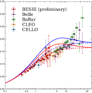
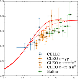
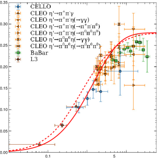
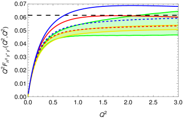
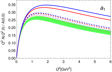
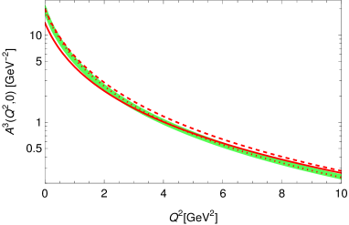
In Fig. 1, the singly virtual TFFs of the pseudoscalar mesons are compared with compiled data. Here we find for CS” an excess in particular for and , which is associated with the fact that the BL limit turns out to be approached from above. This feature disappears in the CS’ model (included by dashed lines). The same behavior shows up in the doubly virtual pion TFF (Fig. 2). Correspondingly the contributions to are also excessive in the CS” model, and no longer compatible with the WP2020 estimate as displayed in the summary table 5.
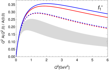
In Fig. 3, the shape of the normalized singly virtual TFF of the meson and also the absolute magnitude of as obtained in the dispersive approach of [52] is compared to the results of the CS”, CS’, and KS models. The KS model considered by us in Ref. [25], which in the sector differs from the CS’ model only with respect to boundary conditions (HW3 instead of HW1), turns out to be closest to the dispersive result, which at large is due to the fact the HW1 result has a result for the decay constant that agrees best with the result for the decay constant MeV from light-cone sum rules [62] used in [52] to constrain the asymptotic behavior. In fact, in the comparison with the unnormalized (lower panel of Fig. 3), the KS(-fit) result is completely within the narrow error band of the dispersive result, for all values of .
In Fig. 4, the shape of the singly virtual TFF of mesons as obtained by a dipole fit of the L3 data [53, 54] is compared with the CS” and CS’ results, showing a good agreement with regard to the slope at small virtualities, but a slower decay at larger ones. Here the KS results are not included in the comparison, because the mixing is too far from the experimental situation.
The doubly virtual TFFs of the axial-vector mesons also determine the branching ratio of decays (see Fig. 5). The results obtained for the CS” and CS’ models listed in Table 4 are fully compatible with the experimental results for obtained by the SND collaboration in Ref. [57]. The CS” result is also compatible with the results of the phenomenological study of Ref. [31, 56] (in particular in the fit with better obtained by leaving out data).
Considering the contribution of the ground-state axial-vector mesons to , the CS” model, which provides a rather good fit of equivalent photon rates and mixing angles for and , yields , incidentally for both the OPE fit and the -fit of . This is significantly lower than the KS(-fit) value of but still way above the WP2020 value of . Since the squared masses of the ground-state axials are all overestimated in the considered models, larger values would be obtained by manually correcting the masses to their experimental values. In the CS”(-fit), where the ground-state axials have the best match with the L3 data, such an extrapolation would give
| (61) |
(In [20], using chiral HW models, we had obtained by manually adjusting rates and masses to experimental values; Ref. [18] estimated this contribution as ; the recent Dyson-Schwinger analysis of Ref. [63] obtained .)
However, the reduction of the contribution from the ground-state axial-vector mesons in the CS” model compared to the KS model is accompanied by a significant increase of the contribution from the tower888The sum over excited axials is carried out using the extrapolation described in [25]. Comparing with an approximate numerical evaluation using the axial bulk-to-bulk propagator we estimate the possible numerical error in the complete sum over the axial-vector towers as +0.45 and for the KS(-fit) model and +0.6 and for the other models. of excited axial-vector mesons, see Table 5. The total contribution from axial-vector mesons is only about 10% below that in the KS(-fit)-model. Including also the contribution from excited pseudoscalars, there is even a net increase.
As already discussed in [24], the two-photon coupling of the first excited pion is much larger than the experimental bound on (according to [9], ), and a similar discrepancy occurs for if this is identified with for which the results from the L3 experiment [54] imply GeV-1. In [24] we interpreted the much larger values appearing for and in Tables 1 and 2 as reflecting the collective effect of the much denser spectrum of excited pseudoscalars in real QCD compared to the HW models. Since these contributions turn out to be rather model dependent, they should perhaps be better viewed as variable parts of the effect of the universal LSDC. In fact, the total sum of contributions from the towers of axials and pseudoscalars shows remarkable stability across the models considered here.
VII Discussion and Conclusions
| KS(OPE fit) | KS(-fit) | CS”(OPE fit) | CS”(-fit) | CS’(OPE fit) | CS’(-fit) | WP2020 | Ref. [64] | |
| 66.1 | 63.4 | 73.3 | 68.8 | 66.6 | 64.3 | 62.6 | ||
| 19.3 | 17.6 | 19.4 | 17.2 | 18.7 | 17.7 | 16.3(1.4) | 14.7(9) | |
| 16.9 | 14.9 | 14.9 | 12.2 | 21.4 | 20.1 | 14.5(1.9) | 13.5(7) | |
| 0.2 | 0.2 | 2.0 | 2.6 | 0.8 | 0.9 | |||
| 1.6 | 1.4 | 3.5 | 3.2 | 1.2 | 0.8 | |||
| 102.3 | 95.9 | 107.6 | 98.2 | 106.7 | 102.1 | 93.8(4.0) | 91.2 | |
| PS poles total | 104 | 97.5 | 113 | 104 | 109 | 104 | ||
| 7.8 | 7.1 | 4.9 | 4.9 | 8.2 | 7.6 | |||
| 20.0 | 17.9 | 12.0 | 12.0 | 20.9 | 18.9 | |||
| 2.2 | 2.4 | 2.5 | 2.3 | 1.7 | 1.7 | |||
| 3.6 | 3.0 | 7.4 | 7.9 | 5.3 | 5.9 | |||
| AV+LSDC total | 33.7 | 30.5 | 26.7 | 27.0 | 36.1 | 34.0 | ||
| AV+P*+LSDC total | 35.5 | 32.1 | 32.2 | 32.8 | 38.2 | 35.7 | 21(16) | |
| total | 138 | 128 | 140 | 131 | 145 | 138 | 115(16.5) |
In Ref. [25] we have considered the KS model [26], where only the standard 5-form part (and this without scalars) is included in the Chern-Simons action and where the U(1)A anomaly is incorporated by a slightly simpler addition to the 5-dimensional Lagrangian. Allowing for a gluon condensate as one further parameter, this gave an excellent match of experimental constraints on the pseudoscalar sector, with masses and photon couplings agreeing with data at the percent level. Evaluating the pseudoscalar TFFs, we found good agreement with phenomenological and lattice results when using a reduced 5-dimensional gauge coupling (-fit) reflecting gluonic corrections, and the resulting HLBL contributions to turned out to agree perfectly with the WP2020 estimates. (However, there is less good agreement with the more recent evaluation of Ref. [64] which has smaller contributions from and , see Table 5.)
In the best-fitting KS(-fit) model, the axial-vector sector, which is responsible for satisfying the longitudinal SDC, was found to contribute ( when excited pseudoscalars are included), slightly larger but consistent with the WP2020 estimate of , see Table 5. However, in the KS model, the axial vector mesons in the sector are found to have stronger deviations from experimental data: the masses of and mesons are 10% and 28% too high, respectively, their mixing angle deviates strongly from experimental findings, and the equivalent photon rates are too high. On the other hand, the combined contribution of and to should be fairly independent of their mixing, and the excesses in masses and photon couplings should partially compensate in .
This points to the need for further refinements, and the improved hQCD models developed in Ref. [29, 48, 49, 32, 33, 34] present several options. However, it is certainly interesting to have alternative hQCD models which also include flavor-symmetry breaking by quark masses and the U(1)A anomaly, while keeping the number of free parameters at a minimum. This is indeed the case with the HW models involving a scalar-extended Chern-Simons term, and we have considered these extensions in two versions, called CS” and CS’ in Table 5, where CS” refers to the case where a scalar potential appears in both terms in (3), while in CS’ this is the case only for the first. (Without any scalar extension, the model is still different from the KS model, but the results are then rather similar.)
Remarkably, both versions improve the results in the axial-vector sector with regard to masses, mixing, and photon couplings. The masses of the ground-state axial-vector mesons are still too high, but only up to +17%; the - mixing angle is close to the experimentally observed ball-park; and the values of determining the equivalent photon rates are almost within the experimental error band for the CS” model (with either full or reduced ). The CS’ model overestimates similarly to the KS model. Since the masses are too high, this should in fact tend to underestimate the contributions of the ground-state axial-vector mesons in the CS” model.
However, the pseudoscalar sector, where the corresponding parameters are nearly perfect in the KS model, shows larger deviations in the photon coupling of mesons, up to -20% in the CS” model and up to +26% in the CS’ one, see Table 2. While the CS’ model has pseudoscalar TFFs that agree similarly well with data than the KS model, they are strongly overestimated at nonzero virtualities in the CS” model, approaching the BL limit from above. In the CS” model, the contribution is thus much higher than the WP2020 estimate, and also the excited pseudoscalars turn out to contribute significantly more than in the other models.
Nevertheless, in the CS” model, the sum of pseudoscalar and axial-vector contributions is almost unchanged compared to the KS model.
Since the KS(-fit) model with reduced provides the best match in the experimentally more constrained pseudoscalar sector, we consider it still the preferred model for making predictions for both pseudoscalar and axial-vector contributions as well as associated LSDC effects in , where the combined contribution from and should be relatively insensitive to their precise octet-singlet mixing. The KS(-fit) model appears also validated by a comparison with the recent dispersive results for the singly virtual TFF (see Fig. 3). We therefore propose to take the range of results added by the CS” and CS’ models as systematic error estimates within the class of HW hQCD models which include flavor-symmetry violating effects999In the soft-wall model of [65] that also includes the strange quark mass and the U(1)A anomaly along the lines of [29], only the pseudoscalar contributions were evaluated; the axial-vector contributions obtained in [47] were obtained in a flavor-symmetric model.. For the complete tower of axial-vector mesons whose longitudinal parts saturate the MV-SDC, we thus obtain for the contributions with -fitted coupling (31)
| (62) |
[The recent estimate obtained in [63] in a DSE/BSE calculation of happens to be fully compatible with this hQCD result.101010Note, however, that the approximations used therein neglect the U(1)A anomaly, which also affects the axial-vector sector in the hQCD models. This is also the case for the simple Regge-like model for axial vector mesons constructed in Ref. [18], which produced an estimate of .]
Adding the excited pseudoscalars (including ), which also contribute to the part of the HLBL tensor that is involved in the MV-SDC, the KS value is somewhat higher and the downward variation is reduced to zero,111111In [24], also the effect of a larger reduction of by 15% instead of 10% was considered, which diminishes the axial-vector contributions by an additional 3%. Including that would give a downward variation of about .
| (63) |
It is presumably this latter result which is to be compared with the WP2020 estimate of for the sum of axial-vector and SDC contributions, as the estimate for the latter involved a model for excited pseudoscalars. It should be noted, however, that the hQCD results only capture fully the LSDC; the SDC for in the symmetric high-momentum limit has the correct behavior, but reaches only 81% of the OPE value.
We would like to recall that the HW hQCD models we have studied are comparatively minimal models. They have just enough free parameters to match , , and quark masses. The coupling , which is usually fixed by the leading-order OPE result for the vector correlator, has been allowed to be replaced by a fit of , which happens to reproduce typical NLO corrections in the vector correlator as well as in TFFs. The only extra freedom introduced was a nonzero value for the gluon condensate that turned out to permit accurate fits of and masses. The three models KS, CS”, and CS’ differ in their implementation of the U(1)A anomaly and whether the bi-fundamental field is included in the Chern-Simons terms. The simpler KS model led to the best fit in the pseudoscalar sector, while the scalar-extended CS” achieved the best fit to and mesons, however at the expense of poor agreement of the TFF with data. However, for the CS” model yields almost the same result as the KS model, which we take as a validation of the results obtained in the latter.
Nevertheless, it would be interesting to see how stable this result is upon further improvements of the hQCD model. In [65], it was found that a simple soft-wall model with a dilaton quadratic in permits a good fit of masses and two-photon couplings of pseudoscalars, but strongly overestimates the TFF, which as in the CS” model approaches the BL limit from above. In fact, in other applications, it was noticed before [66] that soft-wall models are phenomenologically less successful than HW models, and this is also the case with regard to the HVP contribution to [43]. A more promising, but also more difficult alternative is provided by the improved hQCD models in the Veneziano limit of Ref. [29, 48, 49, 32, 33, 34], which permit the implementation of a running coupling and which indeed combine features of hard-wall models through an effective cutoff of the 5-dimensional spacetime with (asymptotically) linear Regge trajectories as in soft-wall models. The results obtained in the present study suggest that a combined high-precision fit of low-energy data in the pseudoscalar and axial-vector sector seems possible, which would improve further the significance of hQCD results for the HLBL contribution to the muon anomalous magnetic moment.
Acknowledgements.
We would like to thank Martin Hoferichter, Elias Kiritsis, Pablo Sanchez Puertas, Peter Stoffer, and Marvin Zanke for helpful discussions. We are particularly grateful to Peter Stoffer for providing the detailed results for the TFF in the dispersive analysis of Ref. [52]. This work has been supported by the Austrian Science Fund FWF, project no. PAT 7221623.Appendix A Relation between and
In this appendix we derive the multiplicative factor relating the tachyon and the HW field . We first list the relevant DBI action and definitions of [29] with reinstated and with having mass dimension 1:
| (64) |
with
| (65) | |||
| (66) | |||
| (67) |
and
| (68) |
The expression is mathematically ambiguous since has both spacetime and flavor indices and needs to be properly defined. The determinant should only act on the spacetime indices. We first pull out a factor of the determinant of the metric to arrive at
| (69) |
with and similar for . In the following, we will ignore the Kalb-Ramond field . We take the second factor to mean
| (70) |
Here means that one should contract spacetime and flavor indices and the trace is only over the spacetime indices. We don’t claim this is the correct full DBI action, we just use this prescription to expand in the lowest orders of . Performing this expansion, one arrives at121212The definitions from before are in the mostly + convention, while the following formula has converted it already to mostly - as in the main text.
| (71) |
The coupling constant is given in terms of the string theory parameters as , where is the volume of possible compact directions that have been integrated out. Upon taking , with the AdS radius we can redefine the tachyon
| (72) |
to arrive at the usual HW action for . The adjoint arises because of the definition (68) compared to our usual conventions for the covariant derivative of the scalar .
Appendix B Quadratic terms and radiative couplings in the Chern-Simons term
In this appendix, we derive more explicit formulas for and , at least when considering pseudoscalar fluctuations of the bi-fundamental scalar only. Many relevant formulas were already derived in [29], but only in the special case of a tachyon background proportional to the identity. As we want to consider a differing strange quark mass, we must generalize these formulas. The exponential in (1) is defined by using the series expansion for the exponential, one crucial difference is that in the matrix multiplication there are extra signs depending on the form degrees of the components, we refer the reader to [29] for the relevant definitions. We start with , which can be extracted from the 2-form part of . We split into background contributions and terms linear in fluctuations. In accordance with (4) and (8) we parameterize fluctuations of the tachyon as .
The background contributions split into terms of different form-degree
| (73) |
The 2 form part of splits into a term containing no and a part containing one . After using the definitions for the multiplication of supermatrices and the supertrace these read
| (74) |
and
| (75) |
This immediately leads to an expression for :
| (76) |
As explained in the main text, any other choice of (which differs by an exact term) can be absorbed in a redefinition of the scalar .
For the computation of , we need to restrict to the 6-form part of . One way of computing is using an explicit formula which reads
| (77) |
where is a one parameter family of connections with and having vanishing curvature.
Since we will only use this part of the action to compute transition functions for mesons which are described by modes that sit in the diagonal parts of the flavor matrices, we can take the fluctuations and the gauge fields to commute with the background . For the one-parameter family of superconnections we take
| (78) |
The superconnection at does not have zero curvature in general, but it does not contain any or terms, which are relevant for radiative decays. Hence the curvature at does not contribute to the processes we consider.
In the above formulas we eventually replace the tachyon background with (4) (we also have ). We stress again that the above formulas are only valid for the meson modes sitting in the diagonal part of the flavor matrices. We note that we have performed no partial integrations to arrive at the above formulas. One may calculate the TFFs for pseudoscalar and axial vector mesons by standard procedures from the above expressions.
In the term one might also suspect radiative couplings (for example of the form ) when considering higher order fluctuations in . Using (77), it is easy to see that no such couplings can be produced (one has to use the 1-parameter family ).
Characteristic for this Chern-Simons term are the factors. They also provide at least a qualitative solution to a potential problem in the study of glueballs decaying into two photons. When considering such processes in models with the non-scalar extended Chern-Simons term one gets a factor of from couplings of flavor-neutral fields to the flavor fields. This could be, for example, a coupling of the Kalb-Ramond field , some RR field , or the metric through the -genus to the flavor gauge fields. The value of depends rather strongly on the number of flavors of quarks one considers, while in real QCD the decay into two photons should not be sensitive to whether there exists a very heavy quark or not. The scalar extended CS term resolves this qualitatively since for a very heavy quark goes to zero very quickly and only contributes at very small , which roughly translates to very high energies.
Appendix C Scalar TFFs
For scalars, the amplitude into two photons can be written as
| (82) |
with
| (83) | |||
| (84) |
This agrees with the results obtained in [67], but there a chiral model was considered, where for . Since we work with nonzero quark masses, we have instead, we get a different asymptotic behavior, namely
| (85) | |||
| (86) |
whereas [67] obtained and , with a different -dependence.
Generalizing the pQCD calculations of Brodsky and Lepage (BL) for the pseudoscalar TFF, the authors of [22] have obtained instead a result with the even weaker fall-off and , where both asymmetry functions are proportional to a function that also appears in the above result in (85) but not in (86).
The OPE of the product of two electromagnetic currents in fact contains a scalar contribution of the form
| (87) |
which is indeed consistent with the holographic result for nonvanishing quark masses. This is not in contradiction with the BL result of [22] and also the slightly older study of [68], since in the limit of one has and the leading terms therein cancel at this symmetric point. However, in contrast to the situation for pseudoscalars and axial vector mesons, there is a contradiction between the BL result and the holographic one away from this point, including the symmetric point with , which is beyond the applicability of the OPE analysis.
As an aside, we would like to mention that a discrepancy between the BL results of [22] and holographic results for TFFs was also found in the case of tensor mesons [47]. However, in this case, there is in fact a difference between the operators involved: on the holographic side the dual operator to the tensor mesons as introduced in [47] is the (flavor-singlet) full energy-momentum tensor, and not actually the operator underlying the analysis of Ref. [22].
Appendix D Evaluation of the electron-positron decay amplitude of axial-vector mesons
In the evaluation of the electron-positron decay amplitude we use the decomposition of the axial-vector TFF (55) in terms of vector meson modes with masses . This decomposition can be derived by inserting the decompositions and
| (88) |
into the expression for . Here the function is a vector meson mode obeying
| (89) |
with normalization such that . If one just straightforwardly takes the decomposition for , and computes one will get something different from (88). The expression that one would obtain in this way would be a sum that diverges at when truncated at any finite mode number. The expression (88) is finite at even when truncating the sum at any finite mode number. To derive (88), we note that obeys the equation
| (90) |
To successfully decompose we should look for modes of this equation. The new modes will, of course, be proportional to , but they will have a nontrivial prefactor to account for their norm. Using , we have
| (91) |
which implies . In order to calculate the inner product between the mode and one of these normed modes, we compute
| (92) | |||
| (93) |
The last equality comes from using the small asymptotics and . Combining all these ingredients one arrives at (88). The expression for then reads
| (94) |
After insertion of (55) into (V.2), one can introduce Feynman parameters for each and perform the integral over the loop variable . In addition, one can integrate out analytically. The result for the quantity in (V.2) is
| (95) |
This integral can be performed numerically to high precision, provided the prescription is properly taken into account. We have crosschecked our numerical results by performing a PV reduction using Feyncalc 9.3.1 [69] and evaluating the standard integrals using LoopTools [70] in Mathematica. Using the PV definitions the integral of the last 3 lines of the previous equation can be expressed as
| (96) |
and directly evaluated using LoopTools.
References
- [1] Muon g-2 Collaboration, D. P. Aguillard et al., Measurement of the Positive Muon Anomalous Magnetic Moment to 0.20 ppm, Phys. Rev. Lett. 131 (2023), no. 16 161802, [arXiv:2308.06230].
- [2] Muon g-2 Collaboration, D. P. Aguillard et al., Detailed report on the measurement of the positive muon anomalous magnetic moment to 0.20 ppm, Phys. Rev. D 110 (2024), no. 3 032009, [arXiv:2402.15410].
- [3] G. Colangelo et al., Prospects for precise predictions of in the Standard Model, arXiv:2203.15810.
- [4] T. Aoyama et al., The anomalous magnetic moment of the muon in the Standard Model, Phys. Rept. 887 (2020) 1–166, [arXiv:2006.04822].
- [5] K. Melnikov and A. Vainshtein, Hadronic light-by-light scattering contribution to the muon anomalous magnetic moment revisited, Phys. Rev. D70 (2004) 113006, [hep-ph/0312226].
- [6] J. Bijnens, N. Hermansson-Truedsson, and A. Rodríguez-Sánchez, Short-distance constraints for the HLbL contribution to the muon anomalous magnetic moment, Phys. Lett. B 798 (2019) 134994, [arXiv:1908.03331].
- [7] J. Bijnens, N. Hermansson-Truedsson, L. Laub, and A. Rodríguez-Sánchez, Short-distance HLbL contributions to the muon anomalous magnetic moment beyond perturbation theory, JHEP 10 (2020) 203, [arXiv:2008.13487].
- [8] G. Colangelo, F. Hagelstein, M. Hoferichter, L. Laub, and P. Stoffer, Short-distance constraints on hadronic light-by-light scattering in the anomalous magnetic moment of the muon, Phys. Rev. D 101 (2020) 051501, [arXiv:1910.11881].
- [9] G. Colangelo, F. Hagelstein, M. Hoferichter, L. Laub, and P. Stoffer, Longitudinal short-distance constraints for the hadronic light-by-light contribution to with large- Regge models, JHEP 03 (2020) 101, [arXiv:1910.13432].
- [10] J. Lüdtke and M. Procura, Effects of longitudinal short-distance constraints on the hadronic light-by-light contribution to the muon , Eur. Phys. J. C 80 (2020), no. 12 1108, [arXiv:2006.00007].
- [11] G. Colangelo, F. Hagelstein, M. Hoferichter, L. Laub, and P. Stoffer, Short-distance constraints for the longitudinal component of the hadronic light-by-light amplitude: an update, Eur. Phys. J. C 81 (2021), no. 8 702, [arXiv:2106.13222].
- [12] M. Knecht, On some short-distance properties of the fourth-rank hadronic vacuum polarization tensor and the anomalous magnetic moment of the muon, JHEP 08 (2020) 056, [arXiv:2005.09929].
- [13] J. Bijnens, N. Hermansson-Truedsson, L. Laub, and A. Rodríguez-Sánchez, The two-loop perturbative correction to the HLbL at short distances, JHEP 04 (2021) 240, [arXiv:2101.09169].
- [14] J. Bijnens, N. Hermansson-Truedsson, and A. Rodríguez-Sánchez, Constraints on the hadronic light-by-light in the Melnikov-Vainshtein regime, JHEP 02 (2023) 167, [arXiv:2211.17183].
- [15] V. Pauk and M. Vanderhaeghen, Single meson contributions to the muon’s anomalous magnetic moment, Eur. Phys. J. C74 (2014) 3008, [arXiv:1401.0832].
- [16] F. Jegerlehner, The Anomalous Magnetic Moment of the Muon, Second Edition, Springer Tracts Mod. Phys. 274 (2017) pp.1–693.
- [17] A. E. Dorokhov, A. P. Martynenko, F. A. Martynenko, A. E. Radzhabov, and A. S. Zhevlakov, The LbL contribution to the muon g-2 from the axial-vector mesons exchanges within the nonlocal quark model, EPJ Web Conf. 212 (2019) 05001, [arXiv:1910.07815].
- [18] P. Masjuan, P. Roig, and P. Sanchez-Puertas, The interplay of transverse degrees of freedom and axial-vector mesons with short-distance constraints in , J. Phys. G 49 (2022), no. 1 015002, [arXiv:2005.11761].
- [19] A. E. Radzhabov, A. S. Zhevlakov, A. P. Martynenko, and F. A. Martynenko, Light-by-light contribution to the muon anomalous magnetic moment from the axial-vector mesons exchanges within the nonlocal quark model, Phys. Rev. D 108 (2023), no. 1 014033, [arXiv:2301.12641].
- [20] J. Leutgeb and A. Rebhan, Axial vector transition form factors in holographic QCD and their contribution to the anomalous magnetic moment of the muon, Phys. Rev. D 101 (2020) 114015, [arXiv:1912.01596].
- [21] L. Cappiello, O. Catà, G. D’Ambrosio, D. Greynat, and A. Iyer, Axial-vector and pseudoscalar mesons in the hadronic light-by-light contribution to the muon , Phys. Rev. D 102 (2020) 016009, [arXiv:1912.02779].
- [22] M. Hoferichter and P. Stoffer, Asymptotic behavior of meson transition form factors, JHEP 05 (2020) 159, [arXiv:2004.06127].
- [23] H. R. Grigoryan and A. V. Radyushkin, Anomalous Form Factor of the Neutral Pion in Extended AdS/QCD Model with Chern-Simons Term, Phys. Rev. D77 (2008) 115024, [arXiv:0803.1143].
- [24] J. Leutgeb and A. Rebhan, Hadronic light-by-light contribution to the muon g-2 from holographic QCD with massive pions, Phys. Rev. D 104 (2021), no. 9 094017, [arXiv:2108.12345].
- [25] J. Leutgeb, J. Mager, and A. Rebhan, Hadronic light-by-light contribution to the muon g-2 from holographic QCD with solved U(1)A problem, Phys. Rev. D 107 (2023), no. 5 054021, [arXiv:2211.16562].
- [26] E. Katz and M. D. Schwartz, An Eta primer: Solving the U(1) problem with AdS/QCD, JHEP 08 (2007) 077, [arXiv:0705.0534].
- [27] T. Schäfer, Euclidean correlation functions in a holographic model of QCD, Phys. Rev. D 77 (2008) 126010, [arXiv:0711.0236].
- [28] D. K. Hong and D. Kim, Pseudo scalar contributions to light-by-light correction of muon in AdS/QCD, Phys. Lett. B680 (2009) 480–484, [arXiv:0904.4042].
- [29] R. Casero, E. Kiritsis, and A. Paredes, Chiral symmetry breaking as open string tachyon condensation, Nucl. Phys. B 787 (2007) 98–134, [hep-th/0702155].
- [30] M. Järvinen, E. Kiritsis, F. Nitti, and E. Préau, Tachyon-dependent Chern-Simons terms and the V-QCD baryon, JHEP 12 (2022) 160, [arXiv:2209.05868].
- [31] M. Zanke, M. Hoferichter, and B. Kubis, On the transition form factors of the axial-vector resonance and its decay into , JHEP 07 (2021) 106, [arXiv:2103.09829].
- [32] I. Iatrakis, E. Kiritsis, and A. Paredes, An AdS/QCD model from Sen’s tachyon action, Phys. Rev. D 81 (2010) 115004, [arXiv:1003.2377].
- [33] I. Iatrakis, E. Kiritsis, and A. Paredes, An AdS/QCD model from tachyon condensation: II, JHEP 11 (2010) 123, [arXiv:1010.1364].
- [34] M. Järvinen and E. Kiritsis, Holographic Models for QCD in the Veneziano Limit, JHEP 03 (2012) 002, [arXiv:1112.1261].
- [35] C. Córdova, D. S. Freed, H. T. Lam, and N. Seiberg, Anomalies in the Space of Coupling Constants and Their Dynamical Applications I, SciPost Phys. 8 (2020), no. 1 001, [arXiv:1905.09315].
- [36] H. Kanno and S. Sugimoto, Anomaly and superconnection, PTEP 2022 (2022), no. 1 013B02, [arXiv:2106.01591].
- [37] P. Kraus and F. Larsen, Boundary string field theory of the D anti-D system, Phys. Rev. D 63 (2001) 106004, [hep-th/0012198].
- [38] T. Takayanagi, S. Terashima, and T. Uesugi, Brane - anti-brane action from boundary string field theory, JHEP 03 (2001) 019, [hep-th/0012210].
- [39] D. Quillen, Superconnections and the Chern character, Topology 24 (1985), no. 1 89–95.
- [40] J. Erlich, E. Katz, D. T. Son, and M. A. Stephanov, QCD and a holographic model of hadrons, Phys. Rev. Lett. 95 (2005) 261602, [hep-ph/0501128].
- [41] L. Da Rold and A. Pomarol, Chiral symmetry breaking from five-dimensional spaces, Nucl. Phys. B721 (2005) 79–97, [hep-ph/0501218].
- [42] Z. Abidin and C. E. Carlson, Strange hadrons and kaon-to-pion transition form factors from holography, Phys. Rev. D 80 (2009) 115010, [arXiv:0908.2452].
- [43] J. Leutgeb, A. Rebhan, and M. Stadlbauer, Hadronic vacuum polarization contribution to the muon g-2 in holographic QCD, Phys. Rev. D 105 (2022), no. 9 094032, [arXiv:2203.16508].
- [44] M. A. Shifman, A. I. Vainshtein, and V. I. Zakharov, QCD and Resonance Physics. Theoretical Foundations, Nucl. Phys. B 147 (1979) 385–447.
- [45] B. Melic, D. Mueller, and K. Passek-Kumericki, Next-to-next-to-leading prediction for the photon to pion transition form-factor, Phys. Rev. D68 (2003) 014013, [hep-ph/0212346].
- [46] F. Hechenberger, J. Leutgeb, and A. Rebhan, Radiative meson and glueball decays in the Witten-Sakai-Sugimoto model, Phys. Rev. D 107 (2023), no. 11 114020, [arXiv:2302.13379].
- [47] P. Colangelo, F. Giannuzzi, and S. Nicotri, Hadronic light-by-light scattering contributions to from axial-vector and tensor mesons in the holographic soft-wall model, Phys. Rev. D 109 (2024), no. 9 094036, [arXiv:2402.07579].
- [48] U. Gürsoy and E. Kiritsis, Exploring improved holographic theories for QCD: Part I, JHEP 02 (2008) 032, [arXiv:0707.1324].
- [49] U. Gürsoy, E. Kiritsis, and F. Nitti, Exploring improved holographic theories for QCD: Part II, JHEP 02 (2008) 019, [arXiv:0707.1349].
- [50] M. Hoferichter, B.-L. Hoid, B. Kubis, S. Leupold, and S. P. Schneider, Dispersion relation for hadronic light-by-light scattering: pion pole, JHEP 10 (2018) 141, [arXiv:1808.04823].
- [51] A. Gérardin, H. B. Meyer, and A. Nyffeler, Lattice calculation of the pion transition form factor with Wilson quarks, Phys. Rev. D 100 (2019), no. 3 034520, [arXiv:1903.09471].
- [52] J. Lüdtke, M. Procura, and P. Stoffer, Dispersion relations for the hadronic VVA correlator, arXiv:2410.11946.
- [53] L3 Collaboration, P. Achard et al., formation in two-photon collisions at LEP, Phys. Lett. B526 (2002) 269–277, [hep-ex/0110073].
- [54] L3 Collaboration, P. Achard et al., Study of resonance formation in the mass region 1400 – 1500 MeV through the reaction , JHEP 03 (2007) 018.
- [55] Particle Data Group Collaboration, S. Navas et al., Review of particle physics, Phys. Rev. D 110 (2024), no. 3 030001.
- [56] M. Hoferichter, B. Kubis, and M. Zanke, Axial-vector transition form factors and , JHEP 08 (2023) 209, [arXiv:2307.14413].
- [57] SND Collaboration, M. N. Achasov et al., Search for direct production of the resonance in collisions, Phys. Lett. B 800 (2020) 135074, [arXiv:1906.03838].
- [58] H. Leutwyler, On the 1/N expansion in chiral perturbation theory, Nucl. Phys. B Proc. Suppl. 64 (1998) 223–231, [hep-ph/9709408].
- [59] R. Escribano and J.-M. Frère, Study of the - system in the two mixing angle scheme, JHEP 06 (2005) 029, [hep-ph/0501072].
- [60] RQCD Collaboration, G. S. Bali, V. Braun, S. Collins, A. Schäfer, and J. Simeth, Masses and decay constants of the and ’ mesons from lattice QCD, JHEP 08 (2021) 137, [arXiv:2106.05398].
- [61] P. Roig and P. Sanchez-Puertas, Axial-vector exchange contribution to the hadronic light-by-light piece of the muon anomalous magnetic moment, Phys. Rev. D 101 (2020) 074019, [arXiv:1910.02881].
- [62] K.-C. Yang, Light-cone distribution amplitudes of axial-vector mesons, Nucl. Phys. B 776 (2007) 187–257, [arXiv:0705.0692].
- [63] G. Eichmann, C. S. Fischer, T. Haeuser, and O. Regenfelder, Axial-vector and scalar contributions to hadronic light-by-light scattering, arXiv:2411.05652.
- [64] S. Holz, M. Hoferichter, B.-L. Hoid, and B. Kubis, A precision evaluation of the - and -pole contributions to hadronic light-by-light scattering in the anomalous magnetic moment of the muon, arXiv:2411.08098.
- [65] P. Colangelo, F. Giannuzzi, and S. Nicotri, , , two-photon transition form factors in the holographic soft-wall model and contributions to , Phys. Lett. B 840 (2023) 137878, [arXiv:2301.06456].
- [66] H. J. Kwee and R. F. Lebed, Pion form-factors in holographic QCD, JHEP 01 (2008) 027, [arXiv:0708.4054].
- [67] L. Cappiello, O. Catà, and G. D’Ambrosio, Scalar resonances in the hadronic light-by-light contribution to the muon (g-2), Phys. Rev. D 105 (2022), no. 5 056020, [arXiv:2110.05962].
- [68] P. Kroll, A study of the – transition form factors, Eur. Phys. J. C 77 (2017), no. 2 95, [arXiv:1610.01020].
- [69] V. Shtabovenko, R. Mertig, and F. Orellana, FeynCalc 9.3: New features and improvements, Comput. Phys. Commun. 256 (2020) 107478, [arXiv:2001.04407].
- [70] T. Hahn and M. Perez-Victoria, Automatized one loop calculations in four-dimensions and D-dimensions, Comput. Phys. Commun. 118 (1999) 153–165, [hep-ph/9807565].