Design of Dedicated Tilt-to-Length Calibration Maneuvers for LISA

Abstract

Tilts of certain elements within a laser interferometer can undesirably couple into measurements as a form of noise, known as Tilt-To-Length (TTL) coupling. This TTL coupling is anticipated to be one of the primary noise sources in the Laser Interferometer Space Antenna (LISA) mission, after Time Delay Interferometry (TDI) is applied. Despite the careful interferometer design and calibration on the ground, TTL is likely to require in-flight mitigation through post-processing subtraction to achieve the necessary sensitivity. Past research has demonstrated TTL subtraction in simulations through the estimation of 24 linear coupling coefficients using a noise minimization approach. This paper investigates an approach based on performing rotation maneuvers for estimating coupling coefficients with low uncertainties. In this study, we evaluate the feasibility and optimal configurations of such maneuvers to identify the most efficient solutions. We assess the efficacy of TTL calibration maneuvers by modulating either the spacecraft (SC) attitude or the Moving Optical Sub-Assembly (MOSA) yaw angle. We found that sinusoidal signals with amplitudes of around $30\text{\,}\mathrm{nrad}\text{/}$ and frequencies near $43\text{\,}\mathrm{mHz}\text{/}$ are practical and nearly optimal choices for such modulations. Employing different frequencies generates uncorrelated signals, allowing for multiple maneuvers to be executed simultaneously. Our simulations enable us to estimate the TTL coefficients with precision below $15\text{\,}\mathrm{\SIUnitSymbolMicro m}\text{/}\mathrm{rad}$ (1-$\sigma$, in free space) after a total maneuver time of $20$ minutes. The results are compared to the estimation uncertainties that can be achieved without using maneuvers.

I Introduction

LISA is a space-based Gravitational Wave (GW) detector that will operate within a measurement band ranging from approximately $0.1\text{\,}\mathrm{mHz}\text{/}$ to $1\text{\,}\mathrm{Hz}\text{/}$ [1]. The detector is composed of three SC, arranged in an almost equilateral triangle with $2.5$ million $\mathrm{km}\text{/}$ arm length, that will trail behind the Earth in a heliocentric orbit. The LISA mission is led by the European Space Agency (ESA) and was recently adopted for an expected launch in the 2030s. Each SC will host two MOSA, each comprising a telescope, an Optical Bench (OB) and a Test Mass (TM). Each MOSA will be pointed towards one of the two remote SC. The MOSA will be designated using the notation shown in Fig. 1, where MOSA $ij$ refers to the assembly on SC $i$ facing SC $j$. The lengths of the three arms of the LISA constellation will vary with time, unlike ground-based GW detectors. This leads to the interferometric measurements being highly affected by laser frequency noise. To mitigate this noise, the TDI [2] algorithm will be applied to generate TDI output variables, which mimic three virtual equal-arm interferometers. In this study we examine the second generation Michelson $X,Y,Z$ combinations. These variables will be affected by TTL coupling, i.e. they contain error terms which depend on the MOSA tilt angles with respect to (w.r.t.) the incident beam. This TTL should be estimated and subtracted from the measurements in post-processing.

In this paper we investigate the possibility of using rotation maneuvers to estimate the TTL coefficients, i.e. the parameters of the TTL model. By injecting a modulation signal into the angles that cause TTL, the signal for the fit is enhanced. This can reduce the uncertainty in the TTL coefficient estimation. This option could be used if TTL is less well separable from other noise terms or GW signals than anticipated. In such a case, the maneuvers could serve as a beneficial backup plan. It may also be decided to perform such maneuvers once within the commissioning phase. TTL maneuvers have already been performed in the LISA Pathfinder (LPF) mission, cf. [3, 4]. A comparable approach has successfully been used in the GRACE Follow-On (GFO) mission and is considered for future geodesy missions as well [wegener_phd, wegener_2020].

Other sources addressing TTL in LISA include [5, 6, 7, 8, 9, 10]. Wanner et al. [5] provide a comprehensive analytical description of TTL in the individual interferometers of LISA as well as in the TDI Michelson variables. In [6] and [7], it is described how the TTL error can be estimated through noise minimization and subtracted from the TDI variables, utilizing pointing angles measured by Differential Wavefront Sensing (DWS) [11]. George et al. [8] apply a Fisher information matrix analysis to derive lower bounds for the uncertainty with which the TTL coefficients can be estimated and use these to analyze the residual TTL noise after post-processing subtraction.

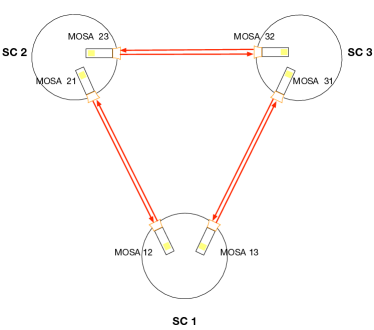
Figure 1: LISA SC constellation, MOSA index notation. Image credit: [6].

In [9], the observability of TTL in the TDI Michelson variables is shown by propagating the TTL contributions through the TDI algorithm. The two options of estimating the TTL coefficients with or without rotation maneuvers are discussed. Periodic maneuvers at frequencies outside the LISA measurement band are considered, in order not to degrade the science measurements. Thus, large amplitudes are required, however, the feasibility of such maneuvers is not discussed. This study is extended in [10] by additionally considering GW signals in the measurements and introducing a separation of TDI variables that allows performing TTL maneuvers without disturbing science operations. The maneuvers discussed in [10] are stochastically generated, instead of periodic stimuli. A quantitative analysis of the estimation error is performed, however, a rather long integration time of $15$ hours was assumed.

This paper follows a different approach of designing dedicated TTL maneuvers, focussing on sinusoidal stimuli at frequencies within the LISA measurement band. We investigate what angular amplitudes are achievable when implemented via SC or MOSA rotations. A detailed analysis of the estimation uncertainty shows a strong dependency on the maneuver frequency, which can be optimized subsequently. In order to maximize the efficiency, we develop a plan to perform several maneuvers simultaneously. This facilitates very good estimation of the TTL coefficients after an integration time of merely $20$ minutes. With simulations we quantify the improvement that such maneuvers provide over the noise minimization approach.

The notation and the TTL model are defined in Sec. II. In Sec. III, the simulator settings are specified. The parameter estimation method is briefly described in Sec. IV. Section V on the maneuver design is the main part of this paper. In particular, we discuss the optimal maneuver frequency, and how multiple maneuvers can be performed simultaneously. The simulation results are reported in Sec. VI.

II Notation

We analyze the TTL in the TDI 2.0 variables $X,Y,Z$, which is the sum of the TTL noise terms of the Inter-Satellite Interferometer (ISI) and the Test Mass Interferometer (TMI). Both are mainly dependent on the $\eta$ (pitch) and $\phi$ (yaw) angles of the MOSA w.r.t. the incident beam. See [5] for more details. Consequently, our model does not distinguish between the two effects. Each angle couples with the local measurement, referred to as Rx TTL coupling, as well as through the measurement on the opposing MOSA located on the distant SC, called Tx TTL coupling. Considering that there are six MOSA, each of which has an $\eta$ and a $\phi$ angle, we evaluate a total of $24$ TTL contributions that transfer to the TDI variables. Owing to the small magnitude of angles, we can linearize the contributions resulting in $24$ linear coupling coefficients. As the coefficients are unknown, it will be necessary to determine them in-flight. The coefficients will also be measured on ground and minimized by aligning the interferometers as precisely as possible. However, they are expected to change during launch, rendering any a priori knowledge of them unreliable.

II.1 MOSA Angles

Let us denote by $\eta_{ij}$ and $\phi_{ij}$ the pitch and yaw angles of MOSA $ij$, $i,j=1,2,3$, $i\neq j$, w.r.t. the incident beam received from SC $j$. These angles describe the combined rotation of MOSA $ij$ w.r.t. SC $i$ and SC $i$ w.r.t. inertial space. The former is represented by the angles $\eta_{ij}^{\mathrm{MOSA}}$ and $\phi_{ij}^{\mathrm{MOSA}}$, respectively. The latter is represented by the roll, pitch, and yaw angles of SC $i$, denoted by $\theta_{i}^{\mathrm{SC}}$, $\eta_{i}^{\mathrm{SC}}$, and $\phi_{i}^{\mathrm{SC}}$. We used the same frame definitions as given for example in [5] or [9], as well as the following small-angle approximations. For $\phi_{ij}$ we have

$$\phi_{ij}\approx\phi_{i}^{\mathrm{SC}}+\phi_{ij}^{\mathrm{MOSA}}.$$ (1)

For $\eta_{ij}$ we have

$$\eta_{ij} \approx\cos(\pi/6)\cdot\eta_{i}^{\mathrm{SC}}\pm\sin(\pi/6)\cdot\theta_{i}^{\mathrm{SC}}+\eta_{ij}^{\mathrm{MOSA}}$$ (2)

$$=\frac{\sqrt{3}}{2}\cdot\eta_{i}^{\mathrm{SC}}\pm\frac{1}{2}\cdot\theta_{i}^{\mathrm{SC}}+\eta_{ij}^{\mathrm{MOSA}},$$ (3)

where the $\pm$ is a plus for $\eta_{13}$, $\eta_{21}$, $\eta_{32}$, and a minus for $\eta_{12}$, $\eta_{23}$, $\eta_{31}$.

We call the DWS measurements of these angles $\eta_{ij}^{\mathrm{DWS}}$ and $\phi_{ij}^{\mathrm{DWS}}$, respectively. These DWS angles contain measurement noise, denoted by $n_{\eta_{ij}}^{\mathrm{DWS}}$ and $n_{\phi_{ij}}^{\mathrm{DWS}}$, respectively. We write this as:

$$\eta_{ij}^{\mathrm{DWS}} =\eta_{ij}+n_{\eta_{ij}}^{\mathrm{DWS}},$$ (4)

$$\phi_{ij}^{\mathrm{DWS}} =\phi_{ij}+n_{\phi_{ij}}^{\mathrm{DWS}}.$$ (5)

For our analyses, the individual DWS sensing noise terms $n_{\eta_{ij}}^{\mathrm{DWS}}$ and $n_{\phi_{ij}}^{\mathrm{DWS}}$ are assumed to be uncorrelated. Further, we assume that there is no cross-talk between $\eta_{ij}^{\mathrm{DWS}}$ and $\phi_{ij}^{\mathrm{DWS}}$, i.e. real angular motion in a pitch angle does not leak into the yaw angle measured by the DWS, nor does real yaw motion leak into DWS pitch measurements.

II.2 TTL in the TDI Variables

Building the TDI variables requires delay operators such as $\mathcal{D}_{ij}$, which accounts for the light travel time from SC $j$ to SC $i$. A cascaded delay operator such as $\mathcal{D}_{ij}\mathcal{D}_{jk}$ applies the delay from SC $k$ to SC $j$ first, followed by the delay from SC $j$ to SC $i$. We use index contraction, where the last index of the left operator is merged with the first index of the right operator. For instance, $\mathcal{D}_{ij}\mathcal{D}_{jk}=\mathcal{D}_{ijk}$, and iteratively $\mathcal{D}_{i\cdots k}\mathcal{D}_{kl}=\mathcal{D}_{i\cdots kl}$, and so on.

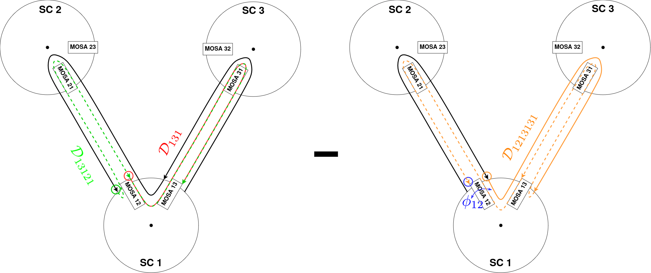
Figure 2: Schematic of the construction of the TDI 2.0 $X$ variable (left minus right combination), cf. [12]. The colors illustrate how to build the TDI angle $\mathcal{X}_{12\phi Rx}$, which is used to define the TTL contribution $X_{12\phi Rx}^{\mathrm{TTL}}$ given in Eq. (7).

The TDI 2.0 variables $X,Y,Z$ are defined for instance in [12] and [13]. Due to the combination of measurements in TDI, each TTL contribution appears with multiple echoes in one TDI variable. Figure 2 illustrates how to construct the TDI 2.0 $X$ variable. We take this as an example to trace the Rx-coupling of the angle $\phi_{12}$ into the TDI $X$ variable. By following the arrows from the points of incidence at MOSA $12$ (marked by colored circles), one can infer the correct delays for the four terms. The terms from the left-hand side (with a “+”) are combined with those from the right-hand side (with a “-”). This way we construct the term

$$\mathcal{X}_{12\phi Rx}=(-{\color[rgb]{0,0,1}1}+{\color[rgb]{1,0,0}\mathcal{D}_{131}}+{\color[rgb]{0,1,0}\mathcal{D}_{13121}}-{\color[rgb]{1,.5,0}\mathcal{D}_{1213131}})\phi_{12},$$ (6)

which we refer to as the TDI angle for the Rx TTL contribution of $\phi_{12}$ in $X$. By multiplying this TDI angle with the TTL coupling coefficient $C_{12\phi Rx}$, one obtains the corresponding TTL contribution, called $X_{12\phi Rx}^{\mathrm{TTL}}$:

$$X_{12\phi Rx}^{\mathrm{TTL}}=C_{12\phi Rx}\cdot\mathcal{X}_{12\phi Rx}.$$ (7)

Note that we consider $X,Y,Z$ in time domain to be in the unit of $\mathrm{m}\text{/}$, so the unit of the TTL is $\mathrm{m}\text{/}$ as well, the unit of the coefficients is $\mathrm{m}\text{/}\mathrm{rad}$, and the unit of the TDI angles is $\mathrm{rad}\text{/}$.

For each of the TTL contributions in $X$, $Y$, and $Z$, we build TDI angles denoted by $\mathcal{X}_{ij\alpha\beta}$, $\mathcal{Y}_{ij\alpha\beta}$, and $\mathcal{Z}_{ij\alpha\beta}$, respectively. Then the individual TTL contributions are given by

$$X_{ij\alpha\beta}^{\mathrm{TTL}} =C_{ij\alpha\beta}\cdot\mathcal{X}_{ij\alpha\beta}$$ (8)

$$Y_{ij\alpha\beta}^{\mathrm{TTL}} =C_{ij\alpha\beta}\cdot\mathcal{Y}_{ij\alpha\beta}$$ (9)

$$Z_{ij\alpha\beta}^{\mathrm{TTL}} =C_{ij\alpha\beta}\cdot\mathcal{Z}_{ij\alpha\beta},$$ (10)

where $i,j\in\{1,2,3\}$, $i\neq j$, $\alpha\in\{\eta,\phi\}$, and $\beta\in\{\mathrm{Rx,Tx}\}$. In total we have $24$ factors $C_{ij\alpha\beta}$, which are called the TTL coupling coefficients and which we assume to be constant in our analysis. The equations for all TTL contributions are provided in Eqs. (62) to (97) in App. A. We write the sum of all TTL contributions in $X$ as

$$X^{\mathrm{TTL}}=\sum\limits_{i,j,\alpha,\beta}X_{ij\alpha\beta}^{\mathrm{TTL}},$$ (11)

where $8$ of $24$ summands are zero, cf. App. A. Likewise, $Y^{\mathrm{TTL}}$ and $Z^{\mathrm{TTL}}$ denote the total TTL in $Y$ and $Z$.

II.3 Data Notation

In this paper we work with simulated sampled data. For the handling of these data and for the parameter estimation we introduce the following compact notation. Let $N$ be the number of considered data points (samples). Throughout this paper, data time series (TS) are represented by vectors and matrices in which the rows are associated with time stamps. For instance, let

$$\eta_{ij}=\begin{pmatrix}\eta_{ij}(t_{1})\\ \eta_{ij}(t_{2})\\ \vdots\\ \eta_{ij}(t_{N})\end{pmatrix}\in\mathbb{R}^{N\times 1},$$ (12)

where the $n^{\mathrm{th}}$ component is $\eta_{ij}(t_{n})$, i.e. the angle at time $t_{n},n=1,\ldots,N$. Other quantities can be written in the same way, e.g., we denote by $X,Y,Z\in\mathbb{R}^{N\times 1}$ the TS of the TDI 2.0 variables, each with $N$ samples.

Table 1: Numbering of TTL contributions, for all index combinations $ij\alpha\beta$ with $i,j=1,2,3$, $i~{}\neq~{}j$, $\alpha~{}\in~{}\{\eta,\phi\}$, and $\beta~{}\in~{}\{\mathrm{Rx},\mathrm{Tx}\}$.

#	1	2	3	4	5	6	7	8	9	10	11	12
Rx	$\eta_{12}$	$\eta_{23}$	$\eta_{31}$	$\eta_{13}$	$\eta_{32}$	$\eta_{21}$	$\phi_{12}$	$\phi_{23}$	$\phi_{31}$	$\phi_{13}$	$\phi_{32}$	$\phi_{21}$
#	13	14	15	16	17	18	19	20	21	22	23	24
Tx	$\eta_{12}$	$\eta_{23}$	$\eta_{31}$	$\eta_{13}$	$\eta_{32}$	$\eta_{21}$	$\phi_{12}$	$\phi_{23}$	$\phi_{31}$	$\phi_{13}$	$\phi_{32}$	$\phi_{21}$

In Tab. 1 we assign a number between $1$ and $24$ to each TTL contribution with indices $ij\alpha\beta$. According to this numbering we define $\mathcal{X}$ to be the $N\times 24$ matrix in which each column is one TDI angle TS $\mathcal{X}_{ij\alpha\beta}~{}\in~{}\mathbb{R}^{N\times 1}$:

$$\mathcal{X}=\begin{pmatrix}\mathcal{X}_{12\eta Rx},&\ldots,&\mathcal{X}_{21\phi Tx}\end{pmatrix}\in\mathbb{R}^{N\times 24},$$ (13)

and accordingly for $\mathcal{Y}\in\mathbb{R}^{N\times 24}$ and $\mathcal{Z}\in\mathbb{R}^{N\times 24}$. Let us denote by $C\in\mathbb{R}^{24\times 1}$ the column vector containing the $24$ true TTL coefficients in the order according to Tab. 1, and by $\hat{C}\in\mathbb{R}^{24\times 1}$ the vector of estimated TTL coefficients. With this notation the entire TTL in $X$ can be written as

$$X^{\mathrm{TTL}} =\sum\limits_{i,j,\alpha,\beta}X_{ij\alpha\beta}^{\mathrm{TTL}}=\sum\limits_{i,j,\alpha,\beta}C_{ij\alpha\beta}\cdot\mathcal{X}_{ij\alpha\beta}$$

$$=\mathcal{X}\cdot C.$$ (14)

Moreover, we define the following concatenated quantities. We denote by $\mathcal{A}$ the concatenation of TDI angle matrices,

$$\mathcal{A}=\begin{pmatrix}\mathcal{X}\\ \mathcal{Y}\\ \mathcal{Z}\end{pmatrix}\in\mathbb{R}^{3N\times 24},$$ (15)

and by $\mathcal{A}^{\mathrm{DWS}}=\mathcal{A}+n_{\mathcal{A}}^{\mathrm{DWS}}$ the measured quantity, derived from DWS angles containing noise. For the TDI variables we define

$$V=\begin{pmatrix}X\\ Y\\ Z\end{pmatrix}\in\mathbb{R}^{3N\times 1}.$$ (16)

Now, the total TTL in the concatenated TDI vector $V$ can be expressed as

$$V^{\mathrm{TTL}} =\begin{pmatrix}X^{\mathrm{TTL}}\\ Y^{\mathrm{TTL}}\\ Z^{\mathrm{TTL}}\end{pmatrix}\in\mathbb{R}^{3N\times 1}$$ (17)

$$=\mathcal{A}\cdot C,$$ (18)

where the right-hand side is a matrix multiplication with $\mathcal{A}\in\mathbb{R}^{3N\times 24}$ and $C\in\mathbb{R}^{24\times 1}$. Since we do not consider any GW signals within this study, we assume that $V$ is the sum of $V^{\mathrm{TTL}}$ and other noise:

$$V=V^{\mathrm{TTL}}+n_{V},$$ (19)

i.e. $n_{V}$ denotes the concatenation of the noise terms in $X,Y,Z$. Assumptions on the noise will be made in Sec. IV on parameter estimation. The most frequently used notation in this paper is summarized in Tab. 2.

Table 2: Summary of the notation used in this paper.

variable	description	dimension	unit
$N$	number of samples	$1$	$1$
$\eta_{ij}$, $\phi_{ij}$	MOSA angles w.r.t. incident beam (TS) $\rightarrow$ Eqs. (1)-(3) and (12)	${N\times 1}$	$\mathrm{rad}\text{/}$
$\eta_{ij}^{\mathrm{DWS}}$, $\phi_{ij}^{\mathrm{DWS}}$	DWS measurements of $\eta_{ij}$, $\phi_{ij}$ (TS) $\rightarrow$ Eqs. (4),(5)	${N\times 1}$	$\mathrm{rad}\text{/}$
$\mathcal{D}_{ij}$	delay operators accounting for the light travel time from SC $j$ to SC $i$	$1$	$1$
$X,Y,Z$	TDI 2.0 variables (TS)	${N\times 1}$	$\mathrm{m}\text{/}$
$\mathcal{X}_{ij\alpha\beta},\mathcal{Y}_{ij\alpha\beta},\mathcal{Z}_{ij\alpha\beta}$	TDI angles for indices $ij\alpha\beta$ in $X,Y,Z$ (TS) $\rightarrow$ Eqs. (8)-(10)	$N\times 1$	$\mathrm{rad}\text{/}$
$C_{ij\alpha\beta}$	true TTL coefficient for indices $ij\alpha\beta$ $\rightarrow$ Eqs. (8)-(10)	$1$	$\mathrm{m}\text{/}\mathrm{rad}$
$X_{ij\alpha\beta}^{\mathrm{TTL}},Y_{ij\alpha\beta}^{\mathrm{TTL}},Z_{ij\alpha\beta}^{\mathrm{TTL}}$	TTL contributions for indices $ij\alpha\beta$ in $X,Y,Z$ (TS) $\rightarrow$ Eqs. (8)-(10)	$N\times 1$	$\mathrm{m}\text{/}$
$X^{\mathrm{TTL}},Y^{\mathrm{TTL}},Z^{\mathrm{TTL}}$	entire TTL in $X,Y,Z$ (TS) $\rightarrow$ Eqs. (11) and (14)	$N\times 1$	$\mathrm{m}\text{/}$
$\mathcal{X},\mathcal{Y},\mathcal{Z}$	TDI angle matrices (each column one TDI angle TS) $\rightarrow$ e.g. Eq. (13)	${N\times 24}$	$\mathrm{rad}\text{/}$
$C$	true TTL coefficients (vector) $\rightarrow$ Eq. (14)	${24\times 1}$	$\mathrm{m}\text{/}\mathrm{rad}$
$\hat{C}$	estimated TTL coefficients (vector)	${24\times 1}$	$\mathrm{m}\text{/}\mathrm{rad}$
$\mathcal{A}$	$=(\mathcal{X}^{T},\mathcal{Y}^{T},\mathcal{Z}^{T})^{T}$ (concatenated matrices) $\rightarrow$ Eq. (15)	${3N\times 24}$	$\mathrm{rad}\text{/}$
$V$	$=(X^{T},Y^{T},Z^{T})^{T}$ (concatenated TS) $\rightarrow$ Eq. (16)	${3N\times 1}$	$\mathrm{m}\text{/}$
$V^{\mathrm{TTL}}$	$=((X^{\mathrm{TTL}})^{T},(Y^{\mathrm{TTL}})^{T},(Z^{\mathrm{TTL}})^{T})^{T}$ (concatenated TS) $\rightarrow$ Eq. (18)	$3N\times 1$	$\mathrm{m}\text{/}$
$n_{V}$	noise in $V$ (concatenated TS) $\rightarrow$ Eq. (19)	$3N\times 1$	$\mathrm{m}\text{/}$

III Simulation

We utilized the Matlab-implemented simulator LISASim [14] to produce simulated LISA data. This includes TTL coupling, DWS measurements, and TDI 2.0 [2] output variables $X,Y,Z$. The analysis of the simulated data was also performed in Matlab.

III.1 Noise in the TDI Variables

Within this study, we do not consider data glitches or GW signals in the TDI variables. The impact of GW signals on the TTL estimation accuracy using the noise minimization approach has been studied in [7] and [15], where no significant impediment has been found. When maneuvers are employed, we expect the estimation to be less vulnerable to disturbances than the noise minimization approach since it is the purpose of the maneuver to produce a TTL signal which stands out of the TTL noise. Large glitches are likely to be infrequent and of very short duration, so that it is expected that they can be removed from the affected data, even if they occur during the maneuver time.

The magnitude of the noise $n_{V}$ in $V$, introduced in Eq. (19), will be required to compute the estimator uncertainties, see also Sec. IV. We generated an Amplitude Spectral Density (ASD) of $n_{V}$ by simulating the TDI output with all TTL coefficients set to zero, which is displayed in Fig. 3. For this reference, the standard deviation of $n_{V}$ at a data sampling rate of $4\text{\,}\mathrm{H}\mathrm{z}$ is

$$\sigma\left(n_{V}\right)\approx$43.5\text{\,}\mathrm{pm}\text{/}$.$$ (20)

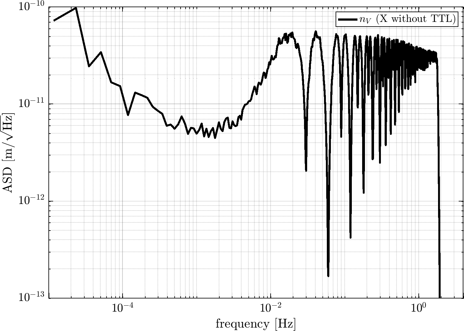
Figure 3: Reference ASD for $X$ without TTL, i.e. $X~{}-~{}X^{\mathrm{TTL}}$. Assuming the spectrum to be identical for $Y$ and $Z$, it also indicates the level of the noise $n_{V}$ in the concatenated TS $V$.

Table 3: The noise levels in LISASim used throughout this analysis.

noise source	noise level in LISASim
clock noise	not implemented
ranging noise	0
SC angular jitter in $\theta^{\mathrm{SC}},\eta^{\mathrm{SC}}$ and $\phi^{\mathrm{SC}}$	$5\text{\,}\mathrm{n}\mathrm{rad}\mathrm{/}\sqrt{\mathrm{Hz}}$
MOSA angular jitter in $\eta^{\mathrm{MOSA}}$ w.r.t SC	$1\text{\,}\mathrm{n}\mathrm{rad}\mathrm{/}\sqrt{\mathrm{Hz}}$
MOSA angular jitter in $\phi^{\mathrm{MOSA}}$ w.r.t SC	$5\text{\,}\mathrm{n}\mathrm{rad}\mathrm{/}\sqrt{\mathrm{Hz}}$
DWS sensing noise at detector level	$70\text{\,}\mathrm{n}\mathrm{rad}\mathrm{/}\sqrt{\mathrm{Hz}}$
beam magnification factor	335
ISI sensing noise	$6.35\text{\,}\mathrm{p}\mathrm{m}\mathrm{/}\sqrt{Hz}$
TMI sensing noise	$1.42\text{\,}\mathrm{p}\mathrm{m}\mathrm{/}\sqrt{Hz}$
RFI sensing noise	$3.32\text{\,}\mathrm{p}\mathrm{m}\mathrm{/}\sqrt{Hz}$
telescope pathlength noise	simulated via thermal expansion with $\mathrm{CTE}=10^{-8}$/K, assuming a telescope optical path length of $0.7\text{\,}\mathrm{m}\text{/}$ and thermal noise as given in [14]. We are aware that the true telescope optical path length is about $1.8\text{\,}\mathrm{m}\text{/}$, see text.
backlink/fibre noise	$3\text{\,}\mathrm{p}\mathrm{m}\mathrm{/}\sqrt{\mathrm{Hz}}$
TM acceleration noise	$2.4\text{\,}\mathrm{f}\mathrm{m}\mathrm{/}\mathrm{s}^{2}\mathrm{/}\sqrt{\mathrm{Hz}}$ (assuming a TM weight of 1.96 kg)
laser frequency noise	$0$ (set to zero because we used TDI and assumed static arm lengths)
$x$ - SC motion	$10\text{\,}\mathrm{n}\mathrm{m}\mathrm{/}\sqrt{\mathrm{Hz}}$

The LISASim settings utilized in this analysis are outlined in Tab. 3. Note that the laser frequency noise was set to zero. We used only post-TDI data, where the laser frequency noise is cancelled due to the static and perfectly known arm lengths assumed by LISASim. The noise term $n_{V}$ introduced above comprises realizations of the noise sources listed in Tab. 3, simulated by LISASim, and propagated through TDI. To ensure consistency, we applied the same settings for all simulations presented in this study. Note that we accidentally assumed the telescope optical path length to be $0.7\text{\,}\mathrm{m}\text{/}$, while the a more realistic value is $1.8\text{\,}\mathrm{m}\text{/}$, however, even with the larger value the effect is still negligible compared to other noise sources. Further, note that the $x$ - SC motion also cancels in the TDI variables.

Before the parameter estimation, a high-pass filter with a cutoff frequency of $1\text{\,}\mathrm{mHz}\text{/}$ was applied to all data, solely to ensure consistent frequency range consideration regardless of the length of the simulated data. The filter had no significant effect on the coefficient estimation. The chosen cutoff frequency is $1\text{\,}\mathrm{mHz}\text{/}$ because TTL dominates the TDI variables only for frequencies above this value.

III.2 Angular Jitter and Noise

For our analysis, it is important to consider the magnitude and spectral shapes of the DWS sensing noise as well as of the jitter in both SC and MOSA. Unless explicitly stated otherwise, the following levels of noise and jitter were implemented for the simulations discussed here:

• DWS noise per angle: $0.2\text{\,}\mathrm{n}\mathrm{rad}\mathrm{/}\sqrt{\mathrm{Hz}}$

• SC jitter in $\phi_{i}^{\mathrm{SC}},~{}\eta_{i}^{\mathrm{SC}},~{}\theta_{i}^{\mathrm{SC}}$: $5\text{\,}\mathrm{n}\mathrm{rad}\mathrm{/}\sqrt{\mathrm{Hz}}$

• MOSA jitter in $\eta_{ij}^{\mathrm{MOSA}}$: $1\text{\,}\mathrm{n}\mathrm{rad}\mathrm{/}\sqrt{\mathrm{Hz}}$

• MOSA jitter in $\phi_{ij}^{\mathrm{MOSA}}$: $5\text{\,}\mathrm{n}\mathrm{rad}\mathrm{/}\sqrt{\mathrm{Hz}}$

These levels refer to ASD levels for frequencies above $3\text{\,}\mathrm{mHz}\text{/}$. The corresponding spectra are presented in Fig. 4. The currently expected DWS sensing noise level at the Quadrant Photodiode (QPD) is $70\text{\,}\mathrm{n}\mathrm{rad}\mathrm{/}\sqrt{\mathrm{Hz}}$. This value must be divided by the beam magnification factor of the telescope [16] of $335$. This results in $70/335$ $\mathrm{n}\mathrm{rad}\mathrm{/}\sqrt{\mathrm{Hz}}$ $\approx$ $0.2\text{\,}\mathrm{n}\mathrm{rad}\mathrm{/}\sqrt{\mathrm{Hz}}$ effective noise in the angles derived from DWS.

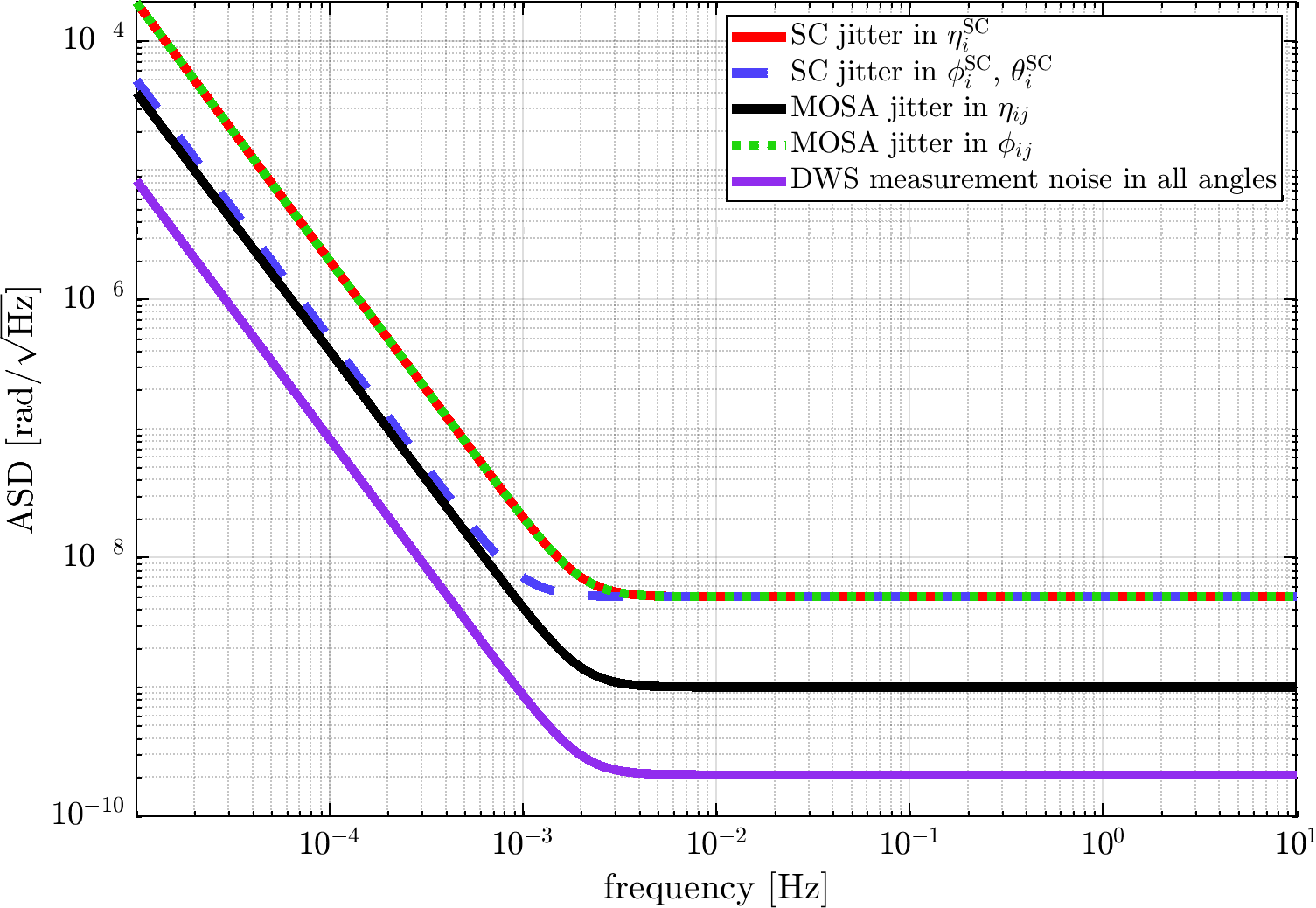
Figure 4: ASD of SC jitter (black, red), MOSA jitter (blue, green), and DWS sensing noise (purple).

The jitter levels were chosen according to the performance model [17] (version of 2021). However, tests with a different simulator, which incorporates a closed Drag Free Attitude Control System (DFACS) control loop, have shown significantly lower MOSA jitter levels. Thus we decided to consider an alternative scenario with reduced MOSA jitter levels of $0.1\text{\,}\mathrm{n}\mathrm{rad}\mathrm{/}\sqrt{\mathrm{Hz}}$ for $\eta_{ij}^{\mathrm{MOSA}}$ and $0.5\text{\,}\mathrm{n}\mathrm{rad}\mathrm{/}\sqrt{\mathrm{Hz}}$ for $\phi_{ij}^{\mathrm{MOSA}}$, in addition to the scenario with the jitter settings listed above. Note that each MOSA is hinged in the yaw axis, but rigid in the pitch axis, so the jitter of the MOSA w.r.t. SC in $\eta$ should be negligible. These reduced MOSA jitter levels will be used for comparison in Sec. VI.

IV Parameter Estimation

We selected a least squares (LSQ) fit in the time domain to estimate the TTL coefficients due to its straightforward implementation and favorable performance. For the LSQ estimation we assume that the terms $n_{V}(t_{n})$ are independent and identically distributed normal random variables with zero mean and variance $\sigma^{2}(n_{V})$, i.e. the three noise terms in $X,Y,Z$ are uncorrelated Gaussian white noise processes. This is a simplification as can be seen in Fig. 3. Furthermore, the LSQ estimator is optimal under the assumption that $n_{\mathcal{A}}^{\mathrm{DWS}}~{}=~{}0$, i.e. that there is no DWS noise, which does not apply to our data. Note that there might be more accurate estimation methods, see for example [18]. However, due to its simplicity the LSQ estimator is a beneficial option for the evaluation of TTL maneuvers.

With the TDI angles $\mathcal{A}^{\mathrm{DWS}}\in\mathbb{R}^{3N\times 24}$ derived from DWS measurements and the concatenated TDI variable $V\in\mathbb{R}^{3N\times 1}$, the approach of the LSQ estimation is to minimize the residual $V-\mathcal{A}^{\mathrm{DWS}}C$ in the least squares sense w.r.t. $C$. I.e., the goal is to minimize the cost function $R$:

$$R(C)= \sum\limits_{n}\left(V(t_{n})-\mathcal{A}^{\mathrm{DWS}}(t_{n})C\right)^{2}$$

$$= \left(V-\mathcal{A}^{\mathrm{DWS}}C\right)^{T}\left(V-\mathcal{A}^{\mathrm{DWS}}C\right)$$

$$= ~{}V^{T}V-2C^{T}\left(\mathcal{A}^{\mathrm{DWS}}\right)^{T}V$$ (21)

$$+C^{T}\left(\mathcal{A}^{\mathrm{DWS}}\right)^{T}\mathcal{A}^{\mathrm{DWS}}C.$$

This expression can be minimized by calculating the derivative w.r.t. $C$,

$$\frac{\partial}{\partial C}R(C)=-2\left(\mathcal{A}^{\mathrm{DWS}}\right)^{T}V+2\left(\mathcal{A}^{\mathrm{DWS}}\right)^{T}\mathcal{A}^{\mathrm{DWS}}C,$$ (22)

and equating it with the zero vector. Hence, the LSQ estimated coefficients are computed as

$$\hat{C}=\left((\mathcal{A}^{\mathrm{DWS}})^{T}\mathcal{A}^{\mathrm{DWS}}\right)^{-1}\left(\mathcal{A}^{\mathrm{DWS}}\right)^{T}V,$$ (23)

see chapter 1 in [19] for some theoretical background.

When assuming zero DWS measurement noise, i.e. if $\mathcal{A}^{\mathrm{DWS}}=\mathcal{A}$, the covariance matrix of $\hat{C}$ is given by

$$\mathrm{cov}\left(\hat{C}\right)=\sigma^{2}(n_{V})\left(\mathcal{A}^{T}\mathcal{A}\right)^{-1}.$$ (24)

Hence, the standard deviations of the estimated coefficients are given by

$$\sigma_{\mathrm{LSQ}}\left(\hat{C}\right)=\sigma(n_{V})\cdot\mathrm{diag}\left(\sqrt{\left(\mathcal{A}^{T}\mathcal{A}\right)^{-1}}\right),$$ (25)

where $\sqrt{\cdot}$ is taken element-wise and diag denotes the column vector of diagonal matrix entries. Note that formula (25), which we also call formal error, may underestimate the true uncertainty since the assumptions of the estimator are not perfectly fulfilled. From a series of statistical tests we have performed, we have concluded that $\sigma_{\mathrm{stat}}$, defined by

$$\sigma_{\mathrm{stat}}:=1.5\cdot\sigma_{\mathrm{LSQ}},$$ (26)

is a value which is very close to the true uncertainty in our simulation setting. These statistical tests are briefly described in App. B.

V Maneuver Design

The aim of TTL calibration maneuvers is to minimize the uncertainty of TTL coefficient estimation by modulating the pitch and yaw angles of the MOSA relative to incident beams. This induces a TTL error, which can be interpreted as a signal instead of noise for the calibration purpose. With the estimated TTL coefficients, the TTL can be subtracted in post-processing. Additionally, the interferometers can be realigned using the Beam Alignment Mechanisms. These BAM will be used for minimizing the TTL already on ground, however, they are planned to be remotely adjustable as well.

The injected signal shall be well distinguishable from the noise background, e.g. with the form of a sine wave or similar, in particular it shall be a repetitive signal with a well defined period $P$. In the frequency domain, such a signal then shows as a peak at $f_{\mathrm{man}}=1/P$, which we call the maneuver frequency. The optimal choice of this frequency for the purpose of estimating TTL coefficients is investigated in detail in Sec. V.1.

For LISA, one option would be to introduce such a modulation signal through the SC attitude, which entails rotating the SC using the cold gas thrusters. Alternatively, the signal can potentially be injected directly into the MOSA angles, specifically rotating the MOSA. Given that the MOSA are designed for angular adjustments in $\phi$, it is expected that such injections via the MOSA are only possible for the $\phi$ angle. These two options are analyzed in Sec. V.2. Afterwards, in Sec. V.3, we fathom ways of performing simultaneous maneuvers. Section V.4 is concerned with an issue that arises when injecting calibration signals into the SC $\phi$ angles.

V.1 Optimal Maneuver Frequency

Since the purpose of TTL maneuvers is to minimize the estimation uncertainty, our approach for optimizing the maneuver frequency is to investigate how it affects the LSQ uncertainty $\sigma_{\mathrm{LSQ}}$ given in Eq. 25. To this end, we examine the formulas for the different TTL contributions given in App. A. In order to reach a quantitative conclusion, we first make some general observations in the following.

We take the TTL contributions of $\eta_{12}$ in $X$ as an example, but the conclusions will hold for all other angles as well. Firstly, note that for the estimation of $C_{12\eta Rx}$ and $C_{12\eta Tx}$, mainly the $X$ variable contains useful information since both contributions are zero in $Z$, and are perfectly correlated to each other in $Y$. I.e., Eqs. (63) and (66) imply:

$$Y_{12\eta Tx}^{\mathrm{TTL}}=\frac{C_{12\eta Tx}}{C_{12\eta Rx}}\cdot Y_{12\eta Rx}^{\mathrm{TTL}}.$$ (27)

This circumstance will be addressed again in Secs. V.3 and V.4 below. Thus, we focus on the $X$ variable in this example.

When assuming constant and equal arm lengths, the following approximations of Eqs. (62) and (65) hold:

$$X_{12\eta\mathrm{Rx}}^{\mathrm{TTL}} \approx C_{12\eta\mathrm{Rx}}\cdot(-1+\mathcal{D}^{2}+\mathcal{D}^{4}-\mathcal{D}^{6})\eta_{12}$$ (28)

$$X_{12\eta\mathrm{Tx}}^{\mathrm{TTL}} \approx C_{12\eta\mathrm{Tx}}\cdot(-1+\mathcal{D}^{2}+\mathcal{D}^{4}-\mathcal{D}^{6})\mathcal{D}^{2}\eta_{12},$$ (29)

where $\mathcal{D}^{2}$ corresponds to a fixed time delay, say $\delta_{t}$, where $\delta_{t}~{}\approx$ $16.7\text{\,}\mathrm{s}\text{/}$. Now, when a periodic signal is injected into $\eta_{12}$, Eq. (28) shows that 4 copies of this signal, all multiplied with the same factor $C_{12\eta Rx}$, will appear in $X$. These echoes can interfere constructively or destructively, which depends on the period of the injected signal. It can be seen immediately that a period corresponding to $\mathcal{D}^{2}$ would result in the first two copies cancelling each other, as well as the last two copies, except for one cycle in the beginning and one cycle in the end. That is, if $P=\delta_{t}$, the TTL contribution in $X$ would almost vanish, rendering the injection useless for TTL calibration. Similarly, with a period of $2\delta_{t}$, term $1$ would cancel with term $3$, and term $2$ with term $4$. In fact, if the period is any fraction $2\delta_{t}/n$, $n\in\mathbb{N}$, the injections will nearly cancel. Note that a period of $2\delta_{t}~{}\approx~{}33.\bar{3}$ $\mathrm{s}\text{/}$ yields a frequency of about $30\text{\,}\mathrm{mHz}\text{/}$. Consequently, all multiples of $30\text{\,}\mathrm{mHz}\text{/}$ are poor choices for the maneuver frequency.

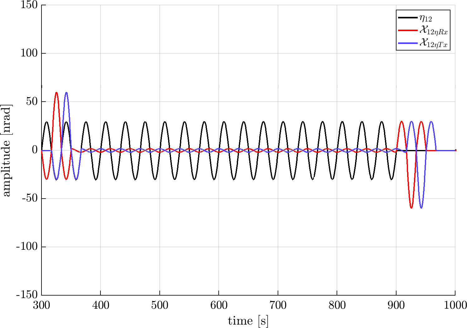
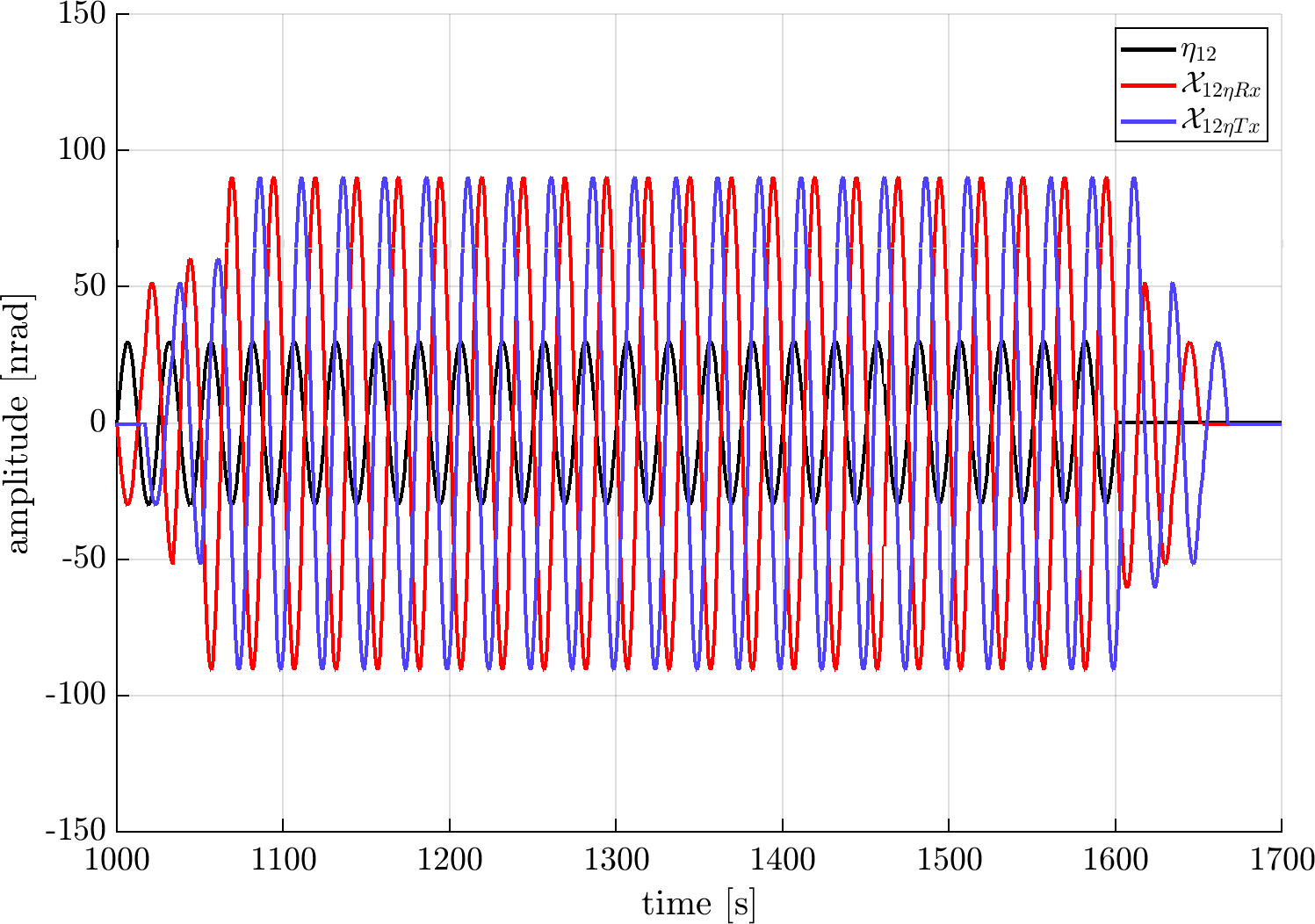
Figure 5: Illustration of bad and good examplary maneuver frequencies. Left ($30\text{\,}\mathrm{mHz}\text{/}$; bad choice): destructive echo interference and high correlation between Rx and Tx contributions in the TDI $X$ variable. Right ($40\text{\,}\mathrm{mHz}\text{/}$; good choice): constructive interference and low correlation. The principle illustrated here for $\eta_{12}$ holds for all other angles as well. Note also that the Rx and Tx contributions in the left plot do not cancel each other entirely because the arm delays were not exactly equal in this simulation.

Figure 5 illustrates simulations of two extreme cases. The black lines show sine waves injected into $\eta_{12}$, with frequencies $30\text{\,}\mathrm{mHz}\text{/}$ (left plot) and $40\text{\,}\mathrm{mHz}\text{/}$ (right plot). The red and blue lines show the TDI angles $\mathcal{X}_{12\eta Rx}$ and $\mathcal{X}_{12\eta Tx}$, respectively, without sensing noise for the purpose of illustration. Note that the TDI angles have not been multiplied by the coefficients and thus have the unit of $\mathrm{rad}\text{/}$, cf. Eq. (6). We make two observations here. Firstly, although both injection signals have the same amplitude, the TDI angles almost vanish in the left plot and are large in the right plot. This is due to the destructive interference for $30\text{\,}\mathrm{mHz}\text{/}$, and the constructive interference for $40\text{\,}\mathrm{mHz}\text{/}$. This observation holds for both Rx and Tx, cf. Eqs. (28) and (29). The second observation is that the correlation between Rx and Tx TDI angles is high for $30\text{\,}\mathrm{mHz}\text{/}$ and low for $40\text{\,}\mathrm{mHz}\text{/}$.

We would like to quantify how these two observations affect the estimation uncertainty. In App. C we derived dependencies of $\sigma_{\mathrm{LSQ}}$ with the simplification made that merely two TTL coefficients are estimated at a time, disregarding potential other correlations, see relation (108). The relevant quantities that depend on the maneuver frequency are the strength of the TDI angle, which can be expressed as $\sigma(\mathcal{X}_{ij\alpha\beta})$, cf. Eq. (102), and the correlation between Rx and Tx TDI angles in $X$:

$$c_{ij\alpha}:=\mathrm{corr}\left(\mathcal{X}_{ij\alpha Rx},\mathcal{X}_{ij\alpha Tx}\right).$$ (30)

Good choices for the frequency of a TTL calibration maneuver can now be deduced from the relation

$$\sigma_{\mathrm{LSQ}}\left(\hat{C}_{ij\alpha\beta}\right)\propto\frac{1}{\sigma\left(\mathcal{X}_{ij\alpha\beta}\right)\cdot\sqrt{1-c_{ij\alpha}^{2}}},$$ (31)

which holds for any $i,j,\alpha$ for which $X$ is the crucial TDI variable. This is the case for all angles on SC $1$, i.e. when $i=1$. For $i=2$, an analog relation holds when $\mathcal{X}$ is replaced by $\mathcal{Y}$. For $i=3$, $\mathcal{X}$ should be replaced by $\mathcal{Z}$.

An interpretation of relation (31) is that larger values of $\sigma(\mathcal{X}_{ij\alpha\beta})$ mean larger calibration signals and hence larger signal-to-noise ratio for the estimation. Secondly, high correlation complicates disentangling the two coefficients and hence increases individual uncertainties. Note that for the derivation of relation (31) it was assumed that only two coefficients, namely $C_{ij\alpha Rx}$ and $C_{ij\alpha Tx}$, are estimated together, so it can merely serve as an approximation in the realistic scenario with $24$ coefficients.

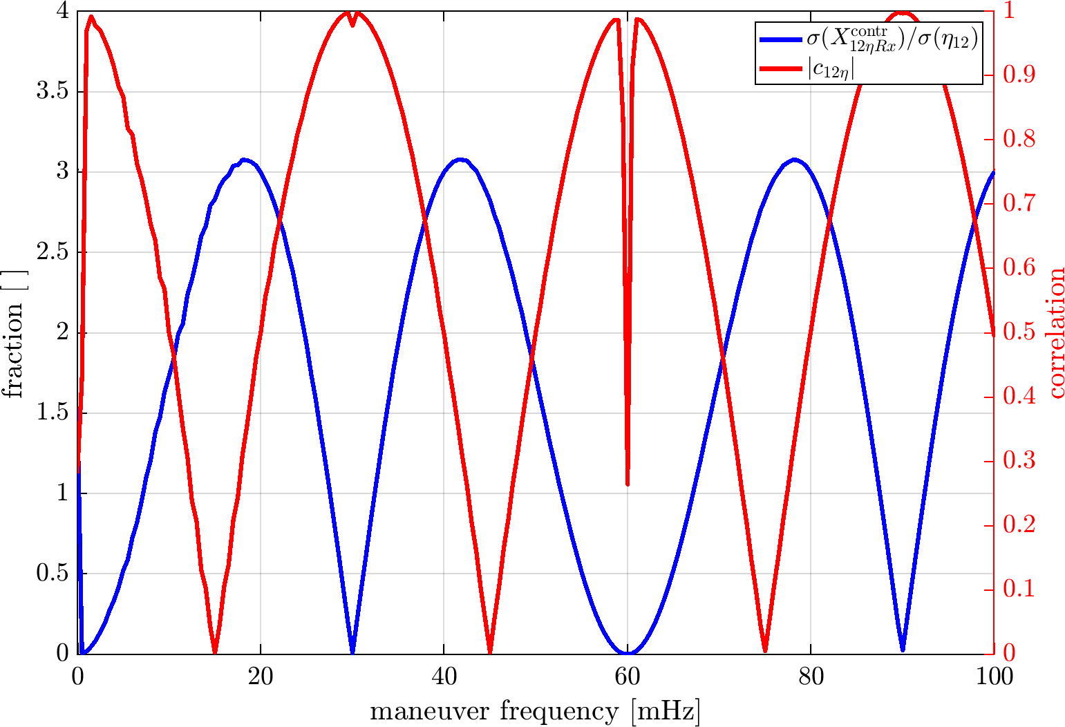
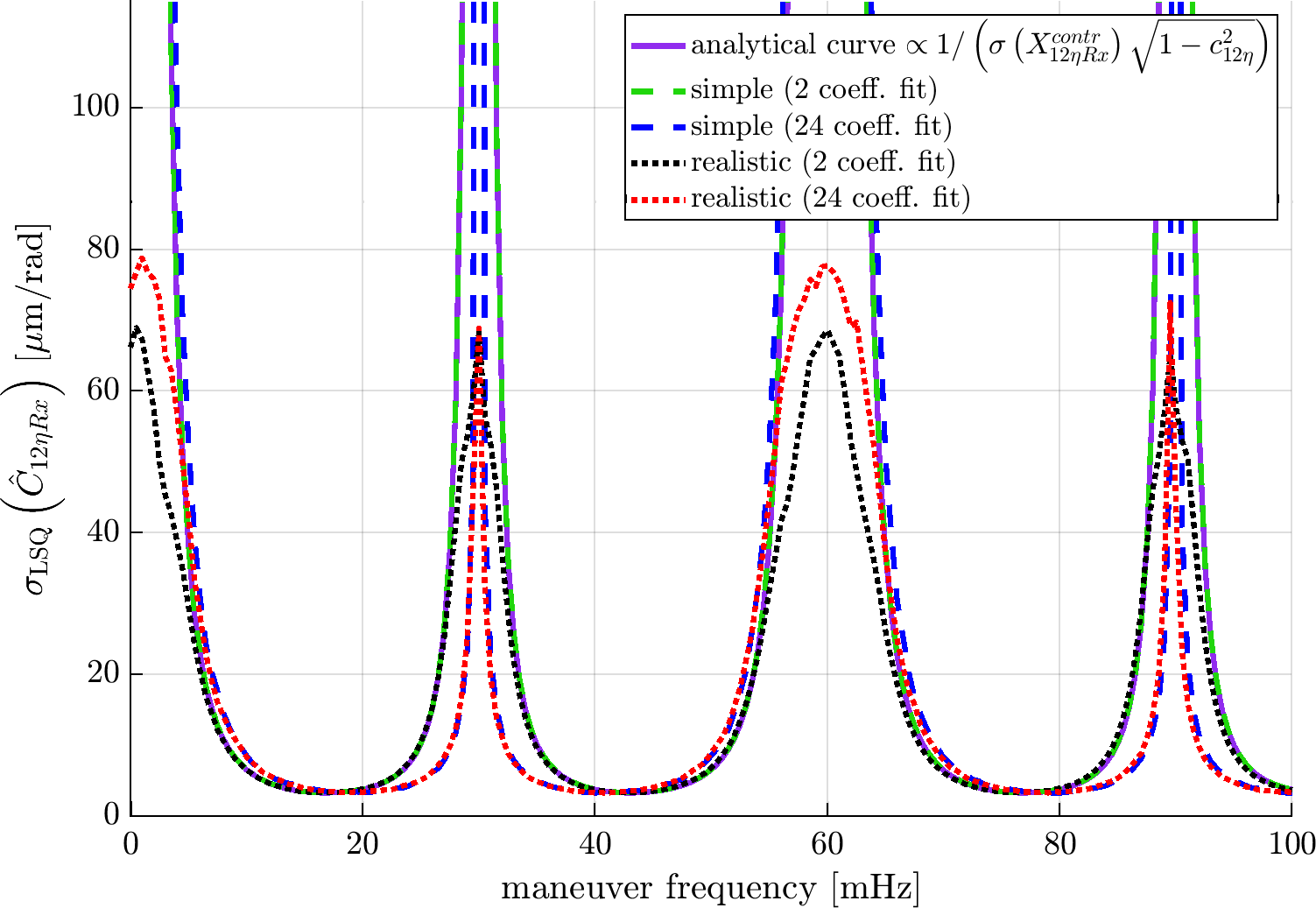
Figure 6: Left: relative standard deviation of the response of an injected signal in a TDI angle (blue line), and absolute value $|c_{12\eta}|$ of the correlation between Rx and Tx TDI angles (red line). Right: $\sigma_{\mathrm{LSQ}}$ depending on maneuver frequency (fixed amplitude) from $60$ simulations (black line) and from the analytical relation (31) (dashed red line).

We tested relation (31) using simulations for $201$ different values of $f_{\mathrm{man}}$ between $0$ and $100\text{\,}\mathrm{mHz}\text{/}$. Each simulation contains one $\eta_{12}$ maneuver with different $f_{\mathrm{man}}$ but fixed amplitude of $100\text{\,}\mathrm{nrad}\text{/}$ and duration of $600\text{\,}\mathrm{s}\text{/}$. For each value of $f_{\mathrm{man}}$ we performed two simulations, a simple and a realistic case. In the realistic case, we used constant simulator settings as defined in Sec. III. In the simple case, we set the DWS noise and all TTL coefficients to zero and all jitter levels to $1$% of the normal level. For each simulation we computed $\sigma(\hat{C}_{12\eta Rx})$ in two ways, firstly by estimating only $C_{12\eta Rx}$ and $C_{12\eta Tx}$, secondly by estimating all $24$ coefficients.

For each simulation with simple settings, we computed $c_{12\eta}$ as well as $\sigma(\mathcal{X}_{12\eta Rx})$. We would prefer the result to be independent of the strength of the injection, which is a different topic addressed in Sec. V.2. Therefore we also computed $\sigma(\eta_{12})$ and examined the normalized signal strength $\sigma(\mathcal{X}_{12\eta Rx})/\sigma(\eta_{12})$. The left plot of Fig. 6 shows this fraction in blue and $|c_{12\eta}|$ in red. From these values an analytical curve $\sigma_{\mathrm{ana}}$ satisfying relation (31) was computed as

$$\sigma_{\mathrm{ana}}=\frac{\sigma(n_{V})}{\sigma(\mathcal{X}_{12\eta Rx})\cdot\sqrt{3N\cdot(1-c_{12\eta}^{2})}},$$ (32)

cf. App. C, with $\sigma(n_{V})~{}=$ $43.5\text{\,}\mathrm{pm}\text{/}$.

The right plot of Fig. 6 shows the estimates of $\sigma_{\mathrm{LSQ}}(\hat{C}_{12\eta Rx})$ obtained in the different ways described above. The analytical curve from Eq. (32) is plotted in purple. The values from estimating either two or all $24$ coefficients in the simple case are depicted as dashed green and blue lines, respectively. The values for the realistic case are shown as dotted black and red lines, respectively. The predicted values are nearly identical to the simple case estimating two coefficients. In all cases, the values strongly increase close to certain maneuver frequencies, e.g. $30\text{\,}\mathrm{mHz}\text{/}$. For the realistic case, this increase is upper bounded due to the angular jitter providing information on the coefficients in addition to the maneuver. In both simple and realistic cases, the form of the spikes deviates from the analytical curve when estimating $24$ coefficients.

We find that the standard deviations of the estimated coefficients, $\sigma(\hat{C}_{ij\alpha\beta})$, is very close to its minimum for maneuver frequencies between $40\text{\,}\mathrm{mHz}\text{/}$ and $45\text{\,}\mathrm{mHz}\text{/}$. We conclude that frequencies between $40\text{\,}\mathrm{mHz}\text{/}$ and $45\text{\,}\mathrm{mHz}\text{/}$ are nearly optimal choices for coefficient estimation, and we chose to use this frequency range for our maneuver simulations. Other good choices exist, e.g. $f_{\mathrm{man}}~{}\approx~{}$$18\text{\,}\mathrm{mHz}\text{/}$ or $f_{\mathrm{man}}~{}\approx$ $78\text{\,}\mathrm{mHz}\text{/}$. On the other hand, $30\text{\,}\mathrm{mHz}\text{/}$ and multiples, more precisely the null frequencies of the TDI transfer function, should be avoided. Note that the optimal frequency is independent of the amplitude of the injection signal.

V.2 Signal Injection

In this section we investigate what injection signals are realistic, in particular what maneuver amplitudes are achievable. We start with injections via SC rotation in Sec. V.2.1, followed by injections via MOSA rotation in Sec. V.2.2.

V.2.1 Injection into SC Angles

The LISA satellites will likely utilize cold gas thrusters for attitude control. Our current best estimate is that these will be similar to the thrusters used in the LPF mission, each of which could produce a maximum force of $500\text{\,}\mathrm{\SIUnitSymbolMicro N}\text{/}$ [20], only part of which was intended for regular use, and part of it was allocated for potentially necessary offsets. We conservatively assume that a force of $F_{\mathrm{max}}=$ $10\text{\,}\mathrm{\SIUnitSymbolMicro N}\text{/}$ per thruster will be available for modulation. The thruster torque is computed as $\tau=r\times F$, where $r$ is the position vector of that thruster w.r.t. the SC center-of-mass (CoM). Since attitude thrusters are activated in pairs, both directed perpendicular to $r$, we may assume a maximum torque of about

$$|\tau_{\mathrm{max}}|=2\cdot|r|\cdot|F_{\mathrm{max}}|\approx$40\text{\,}\mathrm{\SIUnitSymbolMicro N}\text{\,}\mathrm{m}\text{/}$$$ (33)

per satellite axis if the thrusters are located $|r|~{}\approx$ $2\text{\,}\mathrm{m}\text{/}$ away from the SC CoM, which we assume in lack of more detailed specifications. We model the control torque for a maneuver around one principal SC axis by

$$\tau_{\mathrm{man}}(t)=\left|\tau_{\mathrm{max}}\right|\cdot\sin\left(2\pi f_{\mathrm{man}}t\right).$$ (34)

We assume that the SC will be constructed approximately symmetric, and the moments of inertia matrix $J$ will be approximately diagonal with entries $J_{x},J_{y},J_{z}$. Then we can approximate the derivative $\dot{\omega}$ of the angular velocity vector $\omega=(\omega_{x},\omega_{y},\omega_{z})^{T}$ of the SC by

$$\dot{\omega}\approx J^{-1}\tau\approx\begin{pmatrix}\tau_{x}/J_{x}\\ \tau_{y}/J_{y}\\ \tau_{z}/J_{z}\end{pmatrix},$$ (35)

where $\tau$ is the three-dimensional total torque vector acting on the SC. For now, in lack of more detailed specifications, we model the SC as a cylinder with a mass of $2.5\text{\,}\mathrm{t}\text{/}$ and a radius of $2\text{\,}\mathrm{m}\text{/}$, such that $J_{x},J_{y}~{}\approx~{}$$3333\text{\,}\mathrm{kg}\text{\,}{\mathrm{m}}^{2}\text{/}$ and $J_{z}~{}\approx~{}$$5000\text{\,}\mathrm{kg}\text{\,}{\mathrm{m}}^{2}\text{/}$.

A SC Euler angle, e.g. around the $z$ axis, can be approximated by

$$\phi^{\mathrm{SC}}(t) \approx\phi^{\mathrm{SC}}(t_{0})+\int\limits_{t_{0}}^{t}\omega_{z}(s)~{}ds$$

$$=\phi^{\mathrm{SC}}(t_{0})+(t-t_{0})\cdot\omega_{z}(t_{0})+ \int\limits_{t_{0}}^{t}\int\limits_{t_{0}}^{s}\dot{\omega}_{z}(\tilde{s})~{}d\tilde{s}~{}ds$$ (36)

We neglect the constant and the linear term on the right hand side of the equation since they will be removed in data processing by the high-pass filter, cf. Sec. III. Using approximation (35) and inserting the modelled control torque as in Eq. (34), we obtain

$$\phi^{\mathrm{SC}}(t) \approx\frac{1}{J_{z}}\int\limits_{t_{0}}^{t}\int\limits_{t_{0}}^{s}\tau_{\mathrm{man}}(\tilde{s})~{}d\tilde{s}~{}ds$$

$$=\frac{1}{J_{z}}\int\limits_{t_{0}}^{t}\int\limits_{t_{0}}^{s}|\tau_{\mathrm{max}}|\sin(2\pi f\tilde{s})~{}d\tilde{s}~{}ds$$

$$=-\frac{|\tau_{\mathrm{max}}|}{J_{z}(2\pi f)^{2}}\sin(2\pi ft)$$ (37)

for a maneuver around the $z$ axis, and similarly for the $x$ and $y$ axes. We deduce that any SC angle can be modulated by a sinusoid with an amplitude of

$$A_{\mathrm{max}}\approx\frac{$40\text{\,}\mathrm{\SIUnitSymbolMicro N}\text{\,}\mathrm{m}\text{/}$}{$5000\text{\,}\mathrm{kg}\text{\,}{\mathrm{m}}^{2}\text{/}$\cdot(2\pi f)^{2}}\approx$0.2\text{\,}\mathrm{nrad}\text{/}$\cdot\left(\frac{$1\text{\,}\mathrm{Hz}\text{/}$}{f}\right)^{2}.$$ (38)

For a maneuver frequency of $f_{\mathrm{man}}=$ $43\text{\,}\mathrm{mHz}\text{/}$, for instance, we obtain $A_{\mathrm{max}}~{}\approx$ $110\text{\,}\mathrm{nrad}\text{/}$ for a $\phi^{\mathrm{SC}}$ maneuver. Note that the achievable angular amplitude is proportional to $1/f^{2}$. If a maneuver frequency of $20\text{\,}\mathrm{mHz}\text{/}$ would be used, the maximal amplitude would be $500\text{\,}\mathrm{nrad}\text{/}$ for rotations about the $z$ axis, and even larger for rotations about the $x$ or $y$ axes since $J_{z}>J_{x},J_{y}$. We therefore conclude that it is rather conservative to work with a feasible maneuver amplitude of $30\text{\,}\mathrm{nrad}\text{/}$ for maneuver frequencies near $40\text{\,}\mathrm{mHz}\text{/}$.

In Sec. II we have defined $\eta_{ij}$ and $\phi_{ij}$ as the pitch and yaw angles of MOSA $ij$ w.r.t. incident beam. These are the physical angles that cause TTL, so they are to be excited for the TTL calibration. Equations (1) and (3) show how these angles depend on the SC angles. We would like to define a SC rotation that results in a sinusoidal excitation of $\eta_{12}$, ideally without exciting $\eta_{13}$. This is achieved, according to Eq. (3), if

$$\eta_{1}^{\mathrm{SC}}=-\tan(\pi/6)\cdot\theta_{1}^{\mathrm{SC}}=-\frac{1}{\sqrt{3}}\cdot\theta_{1}^{\mathrm{SC}}.$$ (39)

In the other case, for a pure $\eta_{13}$ excitation with $\eta_{12}=0$, one must ensure

$$\eta_{1}^{\mathrm{SC}}=\frac{1}{\sqrt{3}}\cdot\theta_{1}^{\mathrm{SC}}.$$ (40)

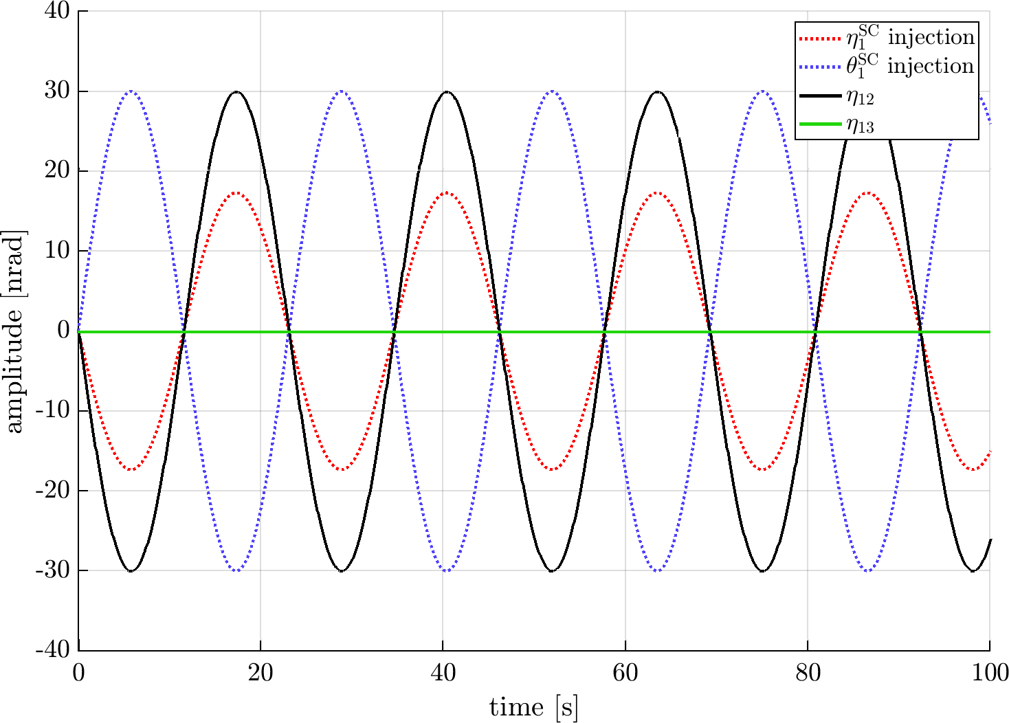
Figure 7: Example: injections into the SC angles $\eta_{1}^{\mathrm{SC}}$ and $\theta_{1}^{\mathrm{SC}}$ result in the depicted $\eta_{12}$ and $\eta_{13}$ angles, cf. Eq. (2). The injections were chosen such that $\eta_{13}=0$.

Figure 7 shows examplary sinusoidal injection signals for the SC angles $\eta_{12}^{\mathrm{SC}}$ and $\theta_{12}^{\mathrm{SC}}$, as well as the $\eta_{12}$ and $\eta_{13}$ angles that result from these injections, cf. Eq. (3). Since the injections were chosen such that Eq. (39) is fulfilled, merely $\eta_{12}$ is excited, while $\eta_{13}=0$.

V.2.2 Injection into MOSA Angles

The MOSA will be controllable with use of the Optical Assembly Tracking Mechanism (OATM). The OATM specifics are not finalized yet, however, one option is to use piezo electric actuators, providing stepwise actuation of each MOSA in the yaw degree of freedom, i.e. around the $z$ axis. Based on internal discussions, we assume here a maximum tracking speed of $5.5\text{\,}\mathrm{nrad}\text{/}\mathrm{s}$ and a motion step resolution of $1\text{\,}\mathrm{nrad}\text{/}$ [21].

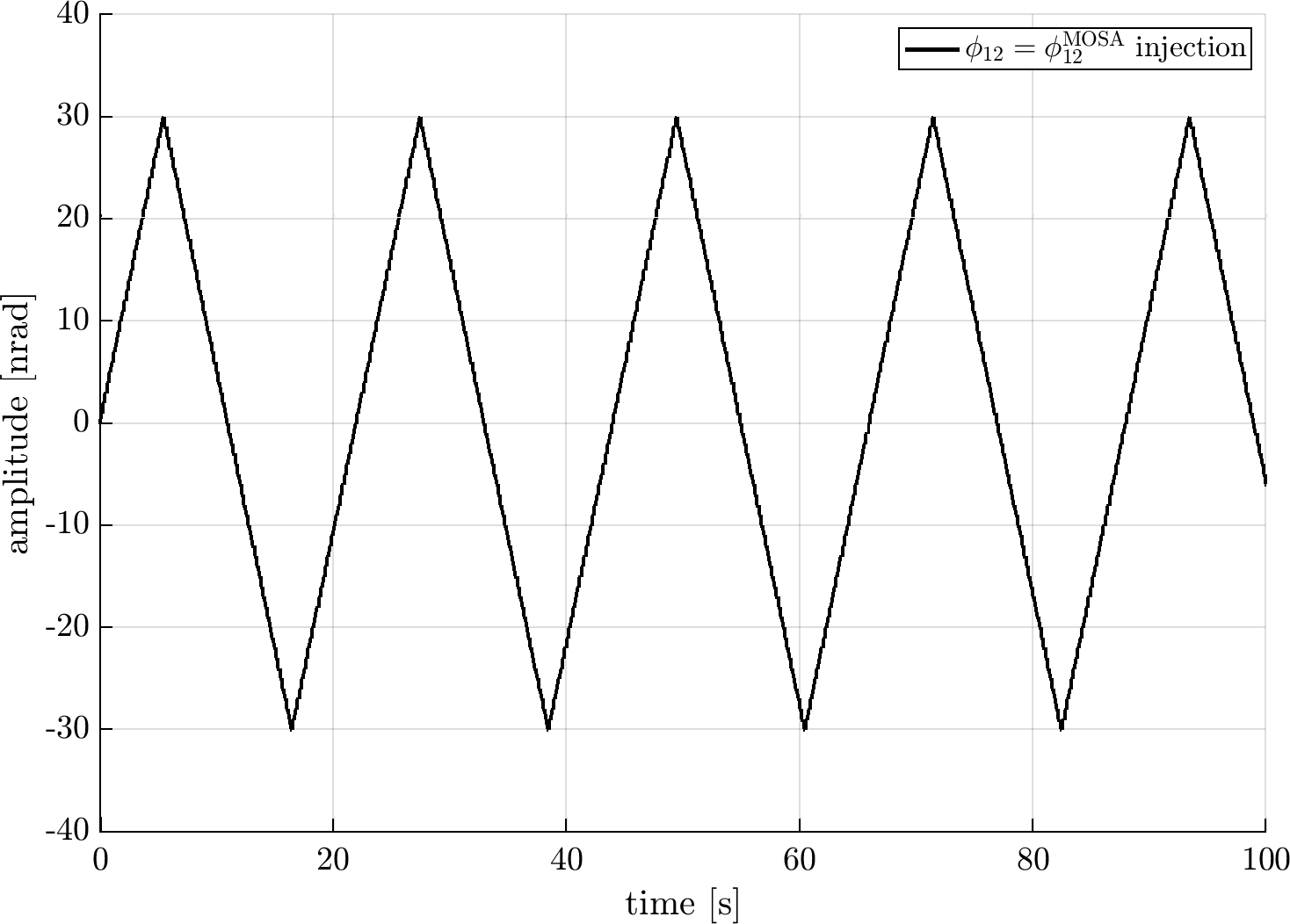
Figure 8: Example: injections directly into the MOSA angle $\phi_{12}^{\mathrm{MOSA}}$ result in the depicted $\phi_{12}$ angle, which is identical to the injection, cf. Eq. (1).

Under these assumptions, a stair-like periodic signal with a triangular shape as shown examplarily in Fig. 8 can be considered feasible. We aim at an angular excitation of $30\text{\,}\mathrm{nrad}\text{/}$ since we used this amplitude here for the maneuvers via SC rotation. Due to the maximum tracking speed of $5.5\text{\,}\mathrm{nrad}\text{/}\mathrm{s}$, the lowest achievable period of such an injection is about $21.8$ seconds, which corresponds to a maneuver frequency of about $45.9\text{\,}\mathrm{mHz}\text{/}$.

Higher frequencies are not feasible if the amplitude shall not be less than $30\text{\,}\mathrm{nrad}\text{/}$. For simplicity, we consider motion steps of $1\text{\,}\mathrm{nrad}\text{/}$, i.e. $30$ steps are required to excite the yaw angle by $30\text{\,}\mathrm{nrad}\text{/}$. For instance, a possible injection signal comprising $25$ cycles within a maneuver duration of $600$ seconds would have a period of $24$ seconds. This would make a signal similar to a sine wave with a frequency of $41.\bar{6}$ $\mathrm{mHz}\text{/}$, i.e. similar to the injection signals that we assume for the SC maneuvers.

Lower frequencies (longer periods) are achievable by slightly delaying each motion step. This way, by using different periods, different uncorrelated injection signals can be created, in analogy to using different frequencies for the sinusoidal SC injections. This will allow for the performance of several MOSA $\phi$ maneuvers simultaneously, cf. Sec. V.3.2 below.

V.2.3 Imperfect Injections

It is important to note that, in this document, it is not investigated in detail how the maneuvers proposed here can be implemented in the real mission. Here the DFACS is assumed to be able to apply the necessary control torques to follow a prescribed commanded set point sequence. Consequently, imperfect injections are not considered here and are subject to further investigations. However, note also that slight deviations from the commanded sequence would not be crucial since the TTL error is depending on the actual $\eta_{ij}$ and $\phi_{ij}$ angles, which are measured by the DWS and used for the fit.

V.3 Simultaneous Maneuver Performance

Table 4: Characterization of TTL contributions in the TDI variables. For each TTL contribution, the variable in which Rx and Tx parts appear uncorrelated is marked in green. In the variables marked in red, Rx and Tx parts appear correlated, while both parts are zero in the variables marked in blue. From this pattern, uncorrelated TTL pairs like $(\eta_{12},\eta_{32})$ can be deduced, for which maneuvers can be performed simultaneously without loss of estimation accuracy.

		appearance of Rx and Tx TTL in TDI
# Rx/Tx $\eta$ ($\phi$)	angle	$X$	$Y$	$Z$
1/13 (7/19)	$\eta_{12}$ ($\phi_{12}$)	uncorrelated	identical	zero
2/14 (8/20)	$\eta_{23}$ ($\phi_{23}$)	zero	uncorrelated	identical
3/15 (9/21)	$\eta_{31}$ ($\phi_{31}$)	identical	zero	uncorrelated
4/16 (10/22)	$\eta_{13}$ ($\phi_{13}$)	uncorrelated	zero	identical
5/17 (11/23)	$\eta_{32}$ ($\phi_{32}$)	zero	identical	uncorrelated
6/18 (12/24)	$\eta_{21}$ ($\phi_{21}$)	identical	uncorrelated	zero

V.3.1 Uncorrelated Pairs

When identical maneuvers are performed in more than one angle simultaneously, in general it might not be possible to disentangle the respective TTL coefficients. In this section we show that there exist pairs of TTL contributions that are naturally uncorrelated, allowing accurate coefficient estimation even if both angles are excited identically. Such pairs can be found by making the following observations regarding the equations given in App. A.

For any given angle, there is always one TDI variable in which both Rx and Tx contributions of this angle are zero. In one of the two remaining TDI variables the Rx and Tx contributions of this angle are perfectly correlated since both appear with identical delays, compare e.g. Eqs. (63) and (66). Thus, for each angle, the main information for coefficient estimation is contained in only one of the three TDI variables $X,Y,Z$.

For instance, for $\eta_{12}$, both Rx and Tx contributions appear in TDI $X$ (uncorrelated), both are zero in $Z$, and both appear in $Y$ (correlated), see Eq. (27). For $\eta_{32}$, the main information is contained in $Z$, but it contributes no TTL to $X$. If $\eta_{12}=\eta_{32}$ for some period such as a maneuver, then each does not disturb the coefficient estimation for the other. In fact, all six $\eta$ angles can be divided this way into three pairs, and analogously for $\phi$. This fact is also shown in [5].

Table 4 shows this pattern for all $\eta$ and $\phi$ angles. This allows to identify pairs of angles for which TTL calibration maneuvers can be performed simultaneously and with identical profile without loss of estimation accuracy: $(\eta_{12},\eta_{32})$, $(\eta_{23},\eta_{13})$, $(\eta_{31},\eta_{21})$, and $(\phi_{12},\phi_{32})$, $(\phi_{23},\phi_{13})$, $(\phi_{31},\phi_{21})$. Note that the same holds for all mixed pairs such as $(\eta_{12},\phi_{32})$, etc.

V.3.2 More than one Pair Simultaneously

The potential drawback of multiple simultaneous maneuvers is that the resulting TTL contributions may be highly correlated, which would result in large estimation uncertainties, cf. App. C. At this point a useful observation is the fact that any two sines having different frequencies are uncorrelated, if both complete an integer number of cycles in the considered time span. Together with the naturally uncorrelated pairs that we found in the previous section, this allows to perform maneuvers for six angles at the same time by using three different frequencies. Hence, it is possible to cover all $12$ angles by performing two times six simultaneous maneuvers instead of $12$ maneuvers in a row. Note that, although not pursued further in this study, two signals with the same frequency but with a relative phase shift of $\pi/2$ would be another example of two uncorrelated signals.

One option would be to perform all six $\phi$ maneuvers at first, using a different maneuver frequency for each of the three pairs $(\phi_{12},\phi_{32})$, $(\phi_{23},\phi_{13})$, and $(\phi_{31},\phi_{21})$. For injections via SC rotations this cannot be done, as will be explained in Sec. V.4. For injections via MOSA rotations it could be achieved by defining three signals as described in Sec. V.2.2, using three different periods. Subsequently all six $\eta$ maneuvers could be performed in the following way. Using Eq. (40), we construct injections into $\theta_{1}^{\mathrm{SC}}$ and $\eta_{1}^{\mathrm{SC}}$ as

$$\theta_{1}^{\mathrm{SC,12inj}}(t) =\sin(2\pi f_{1}t)$$ (41)

$$\eta_{1}^{\mathrm{SC,12inj}}(t) =-\frac{1}{\sqrt{3}}\sin(2\pi f_{1}t),$$ (42)

where the amplitude is set to $1$ for this illustration of principle. Using Eq. (3), we find that the total injected MOSA $\eta$ angles relative to the incident beam are

$$\eta_{12}^{\mathrm{12inj}} =\sin(2\pi f_{1}t)$$ (43)

$$\eta_{13}^{\mathrm{12inj}} =0.$$ (44)

Because relation (39) is satisfied, such SC rotations do not excite $\eta_{13}$. Additionally, another rotation can be constructed which excites $\eta_{13}$, but not $\eta_{12}$, by

$$\theta_{1}^{\mathrm{SC,13inj}}(t) =\sin(2\pi f_{2}t)$$ (45)

$$\eta_{1}^{\mathrm{SC,13inj}}(t) =\frac{1}{\sqrt{3}}\sin(2\pi f_{2}t),$$ (46)

using a second frequency $f_{2}$, resulting in the following MOSA injection angles:

$$\eta_{12}^{\mathrm{13inj}} =0$$ (47)

$$\eta_{13}^{\mathrm{13inj}} =\sin(2\pi f_{2}t).$$ (48)

The two rotations can be added up to obtain simultaneous uncorrelated signals in the two MOSA $\eta$ angles:

$$\eta_{12} =\sin(2\pi f_{1}t)$$ (49)

$$\eta_{13} =\sin(2\pi f_{2}t).$$ (50)

An example of such an injection is shown in Fig. 9. Clearly, this can be done analogously for SC $2$ and SC $3$. It can be seen that this type of injection in fact requires exciting $\theta_{1}^{\mathrm{SC}}$ to amplitudes larger than $30\text{\,}\mathrm{nrad}\text{/}$, which we excluded above. Therefore we consider another option in the following.

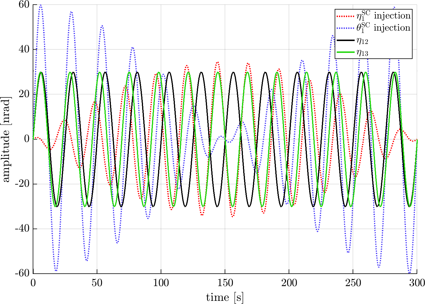
Figure 9: Example: simultaneous $\eta_{12}$ and $\eta_{13}$ maneuvers using two sinusoidal injections with different frequencies, $f_{1}~{}=$ $40\text{\,}\mathrm{mHz}\text{/}$ and $f_{2}~{}=~{}43.\bar{3}$ $\mathrm{mHz}\text{/}$.

Another way to implement two times six maneuvers to cover all $12$ angles is to include mixed uncorrelated pairs. I.e., it is possible to rotate one of the MOSA in $\eta$ via SC injection, while the other MOSA on the same SC is rotated in $\phi$ via MOSA injection. In the scenario which we will call case A, we chose to excite $(\eta_{12},\eta_{32})$ with a frequency $f_{1}$, $(\eta_{21},\phi_{31})$ with $f_{2}$, and $(\phi_{13},\phi_{23})$ with $f_{3}$. Subsequently the pairs $(\phi_{12},\phi_{32})$ $(\phi_{21},\eta_{31})$, and $(\eta_{13},\eta_{23})$ were excited using the same three frequencies $f_{1},f_{2},f_{3}$, respectively. Note that this is one of many possible configurations. Figure 10 examplarily shows simultaneous injections for SC $1$.

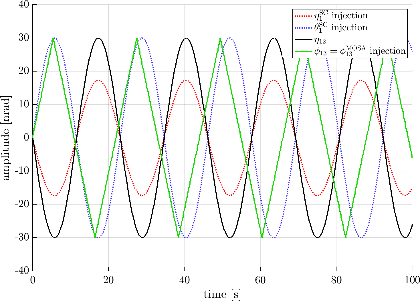
Figure 10: Example: sinusoidal $\eta_{12}$ SC maneuver with $f_{1}~{}=~{}43.\bar{3}$ $\mathrm{mHz}\text{/}$, and simultaneous $\phi_{13}$ MOSA maneuver with triangular shape and $f_{2}~{}=$ $45\text{\,}\mathrm{mHz}\text{/}$, respectively.

V.4 Issue with SC Phi Injections

The procedure to excite one MOSA’s $\eta$ angle via SC rotation, while the other MOSA’s $\eta$ angle is unaffected, as described in Sec. V.2.1 and depicted in Fig.7, is not feasible for the $\phi$ angles. In this section we discuss the impact of this fact on the TTL calibration via injection into SC angles.

V.4.1 Problem Statement

Equation (1) shows that any rotation of SC $i$ in the yaw angle $\phi_{i}^{\mathrm{SC}}$ necessarily causes identical rotations of $\phi_{ij}$ and $\phi_{ik}$, $j\neq k$. Exciting $\phi_{i}^{\mathrm{SC}}$ thereby stimulates four TTL contributions, i.e. the Rx and Tx contributions from the two local MOSA’ $\phi$ angles. Taking $\phi_{1}^{\mathrm{SC}}$ as an example, this means that the coefficients $C_{12\phi Rx}$, $C_{12\phi Tx}$, $C_{13\phi Rx}$, and $C_{13\phi Tx}$ are involved. The TTL contributions associated with these coefficients can be obtained from Eqs. (62), (63), (80), (82), (65), (66), (83), and (85) by replacing all $\eta$’s with $\phi$’s. Since we consider calibration signals injected into $\phi_{1}^{\mathrm{SC}}$, we assume for the moment $\phi_{12}~{}\approx~{}\phi_{1}^{\mathrm{SC}}~{}\approx~{}\phi_{13}$, neglecting the differential MOSA jitter in $\phi_{12}^{\mathrm{MOSA}}$ and $\phi_{13}^{\mathrm{MOSA}}$, only considering common MOSA motion caused by SC rotation.

The terms in the TDI $X$ variable depending on $C_{12\phi Rx}$ and $C_{13\phi Rx}$ differ only due to different armlengths, and similarly for $C_{12\phi Tx}$ and $C_{13\phi Tx}$. If one assumes almost equal armlengths, one can approximate the sum of TTL contributions in TDI $X$ due to $\phi_{1}^{\mathrm{SC}}$ as

$$X_{\phi_{1}^{\mathrm{SC}}}^{\mathrm{TTL}} \approx[(C_{13\phi Rx}-C_{12\phi Rx})\cdot(1-\mathcal{D}^{2}-\mathcal{D}^{4}+\mathcal{D}^{6})$$ (51)

$$+(C_{13\phi Tx}-C_{12\phi Tx})\cdot(\mathcal{D}^{2}-\mathcal{D}^{4}-\mathcal{D}^{6}+\mathcal{D}^{8})]\phi_{1}^{\mathrm{SC}},$$

where $\mathcal{D}$ is a one-arm delay, as in approximations (28) and (29). Then $X$ allows only to estimate the differences $(C_{13\phi Rx}-C_{12\phi Rx})$ and $(C_{13\phi Tx}-C_{12\phi Tx})$.

In Sec. V.1 we have seen that the Rx and Tx TTL contributions of $\phi_{12}$ in $Y$ are perfectly correlated, cf. Eq. (27). The same is true for the contributions of $\phi_{13}$ in $Z$. This implies that, from the $Y$ and $Z$ variables, one can only estimate the combinations $(C_{12\phi Rx}+C_{12\phi Tx})$ and $(C_{13\phi Rx}+C_{13\phi Tx})$, but not the individual coefficients.

In total, we can estimate the right-hand side $\tilde{C}$ of

$$\begin{pmatrix}-1&1&0&0\\ 0&0&-1&1\\ 1&0&1&0\\ 0&1&0&1\end{pmatrix}\cdot\begin{pmatrix}C_{12\phi Rx}\\ C_{13\phi Rx}\\ C_{12\phi Tx}\\ C_{13\phi Tx}\end{pmatrix}=\tilde{C}.$$ (52)

Since the matrix on the left-hand side has rank 3, it is not possible to determine the 4 individual coefficients from the mere knowledge of $\tilde{C}$.

V.4.2 Correlation with Unequal Armlengths

Above we have seen that SC $\phi$ maneuvers do not allow the estimation of the individual $\phi$ TTL coefficients, assuming that the three LISA arms have equal length. Here we examine if this conclusion still holds when we consider unequal arm lengths. For the duration of a maneuver, assume that $\phi_{1}^{\mathrm{SC}}$ is dominated by the sinusoidal injection signal, i.e.

$$\phi_{1}^{\mathrm{SC}}=\sin(\omega t)=\sin(2\pi f_{\mathrm{man}}t).$$ (53)

The crucial quantity is the correlation between Eqs. (62) and (80) since the perfect correlations in $Y$ and $Z$ hold independent of the armlengths. For simplicity we assume static armlengths for a short period such as the maneuver time, so that the delay operators are commutative. Then one can show that

$$\left|\mathrm{corr}(X_{12\phi Rx}^{\mathrm{TTL}},X_{13\phi Rx}^{\mathrm{TTL}})\right| \geq\left|\mathrm{corr}\left(D_{121}\phi_{1}^{\mathrm{SC}},D_{131}\phi_{1}^{\mathrm{SC}}\right)\right|$$

$$=\left|\mathrm{corr}\left(\sin(\omega t),\sin(\omega(t-\delta_{t}))\right)\right|$$

$$=\left|\cos\left(\omega\delta_{t}\right)\right|,$$

where $\delta_{t}$ denotes the differential time between the delays $D_{131}$ and $D_{121}$. The correlation is $1$ for $\omega\delta_{t}=0$ and $0$ for $\omega\delta_{t}=\pi/2$. If, for instance, $f_{\mathrm{man}}~{}=$ $40\text{\,}\mathrm{mHz}\text{/}$, the correlation is $0$ for $\delta_{t}~{}=$ $6.25\text{\,}\mathrm{s}\text{/}$, which will never occur. For $\delta_{t}~{}\approx$ $0.167\text{\,}\mathrm{s}\text{/}$, which corresponds to a $1$ % armlength difference, we have

$$\left|\mathrm{corr}\left(X_{12\phi Rx}^{\mathrm{TTL}},X_{13\phi Rx}^{\mathrm{TTL}}\right)\right|>0.999.$$ (54)

That is, for the purpose of TTL maneuver injections into the $\phi_{1}^{\mathrm{SC}}$ angle, the terms $X_{12\phi Rx}^{\mathrm{TTL}}$ and $X_{13\phi Rx}^{\mathrm{TTL}}$, as well as the terms $X_{12\phi Tx}^{\mathrm{TTL}}$ and $X_{13\phi Tx}^{\mathrm{TTL}}$, can be considered almost perfectly correlated. The same holds for SC $2$ and SC $3$ as well. If the armlength difference was $5$ % instead of $1$ %, the respective absolute correlation would still be larger than $0.98$. This shows that SC maneuvers in $\phi$ are impractical for the estimation of TTL coefficients.

V.4.3 Workaround

A potential way to circumvent the problem discussed above is to utilize MOSA maneuvers via the OATM. In Sec. V.2.2 above, it is described what MOSA maneuvers are feasible and how different uncorrelated injection signals can be obtained. The results of a full simulation, comprising SC maneuvers for the $\eta$ angles and MOSA maneuvers for the $\phi$ angles, are presented in Sec. VI.1.

V.4.4 Subtraction without Knowledge of Individual Coefficients

Knowledge of the coefficient combinations defined by the left hand side of Eq. 52 is sufficient in order to subtract TTL from the TDI variables. This was confirmed with simulations and the results are presented in Sec. VI.3.

VI Simulation Results

VI.1 Full Simulation with Maneuvers (case A)

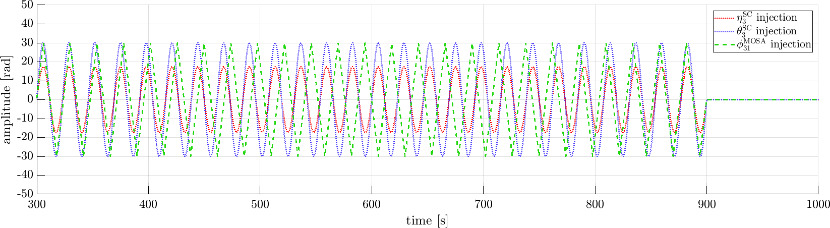
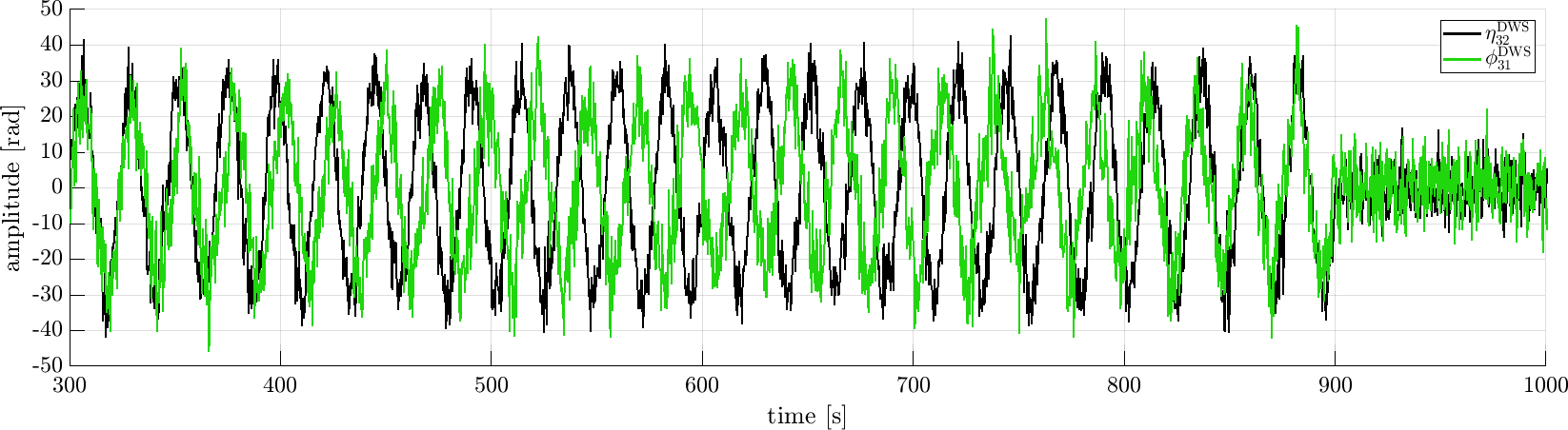
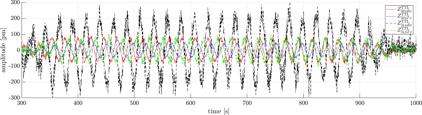
Figure 11: $\eta_{32}$ and $\phi_{31}$ maneuvers from the full simulation. Top: angle injections; Middle: simulated DWS angles; Bottom: resulting TTL contributions in TDI $Z$.

We performed a full simulation, called case A, comprising maneuvers for all angles. The simulation was performed in Matlab with the LISASim simulator [14]. Noise and jitter levels were chosen according to Sec. III. The full MOSA jitter was applied: $1\text{\,}\mathrm{n}\mathrm{rad}\mathrm{/}\sqrt{\mathrm{Hz}}$ for $\eta$ and $5\text{\,}\mathrm{n}\mathrm{rad}\mathrm{/}\sqrt{\mathrm{Hz}}$ for $\phi$. The true TTL coupling coefficients were uniformly distributed random values between $-3\text{\,}\mathrm{mm}\text{/}\mathrm{rad}$ and $3\text{\,}\mathrm{mm}\text{/}\mathrm{rad}$. The estimated coefficients and their uncertainties were obtained by a LSQ fit in the time domain, as described in Sec. IV. In total $2000\text{\,}\mathrm{s}\text{/}$ of data were simulated, while the first and last $300\text{\,}\mathrm{s}\text{/}$ were cut off to remove potential filter effects, so the integration time for estimation was $T~{}=$ $1400\text{\,}\mathrm{s}\text{/}$.

We defined two sets of maneuvers, where we used mixed uncorrelated pairs and employed three different frequencies. This approach was described in Sec. V.3.2. The modulations in $\eta$ were sinusoidal injections via SC angles, cf. Sec. V.2.1. For $\phi$ we used triangular-shaped signals injected into the MOSA yaw angles, cf. Sec. V.2.2. In the first set, $(\eta_{12},\eta_{32})$ were excited at a frequency $f_{1}~{}=~{}43.\bar{3}$ $\mathrm{mHz}\text{/}$, $(\eta_{21},\phi_{31})$ at $f_{2}~{}=~{}41.\bar{6}$ $\mathrm{mHz}\text{/}$, and $(\phi_{13},\phi_{23})$ at $f_{3}~{}\approx~{}44.7$ $\mathrm{mHz}\text{/}$. The second set comprised maneuvers in $(\phi_{12},\phi_{32})$ at $f_{3}$, $(\phi_{21},\eta_{31})$ at $f_{2}$, and $(\eta_{13},\eta_{23})$ at $f_{1}$.

The first set of maneuvers started at $t_{0}~{}=$ $300\text{\,}\mathrm{s}\text{/}$, the second set started at $t_{0}~{}=$ $1000\text{\,}\mathrm{s}\text{/}$, each set comprising six simultaneous maneuvers with a duration of $T_{\mathrm{man}}~{}=$ $600\text{\,}\mathrm{s}\text{/}$. $100\text{\,}\mathrm{s}\text{/}$ after each set of maneuvers was used additionally for the estimation to capture the entire effect of the maneuvers in the TDI variables, including delayed terms. Thus, the total integration time for estimation was $T~{}=$ $1400\text{\,}\mathrm{s}\text{/}$. All maneuvers had an injection amplitude of $A_{\mathrm{man}}~{}=$ $30\text{\,}\mathrm{nrad}\text{/}$. Table 5 lists all maneuver parameters including the maneuver frequencies.

Table 5: Maneuver parameters for the full simulation

set	angle	$t_{0}$ [$\mathrm{s}\text{/}$]	$T_{\mathrm{man}}$ [$\mathrm{s}\text{/}$]	$A_{\mathrm{man}}$ [$\mathrm{nrad}\text{/}$]	$f_{\mathrm{man}}$ [$\mathrm{mHz}\text{/}$]	P [$\mathrm{s}\text{/}$]
$1$	$\eta_{12}$	$300$	$600$	$30$	$43.\bar{3}$	$23.08$
$1$	$\eta_{32}$	$300$	$600$	$30$	$43.\bar{3}$	$23.08$
$1$	$\eta_{21}$	$300$	$600$	$30$	$41.\bar{6}$	$24$
$1$	$\phi_{31}$	$300$	$600$	$30$	$41.\bar{6}$	$24$
$1$	$\phi_{13}$	$300$	$604$	$30$	$44.7$	$22.36$
$1$	$\phi_{23}$	$300$	$604$	$30$	$44.7$	$22.36$
$2$	$\phi_{12}$	$1000$	$604$	$30$	$44.7$	$22.36$
$2$	$\phi_{32}$	$1000$	$604$	$30$	$44.7$	$22.36$
$2$	$\phi_{21}$	$1000$	$600$	$30$	$41.\bar{6}$	$24$
$2$	$\eta_{31}$	$1000$	$600$	$30$	$41.\bar{6}$	$24$
$2$	$\eta_{13}$	$1000$	$600$	$30$	$43.\bar{3}$	$23.08$
$2$	$\eta_{23}$	$1000$	$600$	$30$	$43.\bar{3}$	$23.08$

Figure 11 illustrates the $\eta_{32}$ and $\phi_{31}$ maneuvers, with maneuver parameters as specified in Tab. 5. The top plot shows the injections into $\eta_{3}^{\mathrm{SC}}$ and $\theta_{3}^{\mathrm{SC}}$ to excite $\eta_{32}$ and into $\phi_{31}^{\mathrm{MOSA}}$ to excite $\phi_{31}$. The DWS measurements of the excited angles are displayed in the middle plot, where it can be seen that the correlation between $\eta_{32}$ and $\phi_{31}$ is minimal due to the two different frequencies. The bottom plot shows the four TTL contributions which result from these angular injections, i.e. $Z_{32\eta Rx}^{\mathrm{TTL}}$, $Z_{32\eta Tx}^{\mathrm{TTL}}$, $Z_{31\phi Rx}^{\mathrm{TTL}}$, and $Z_{31\phi Tx}^{\mathrm{TTL}}$. The amplitudes of the TTL terms are not equal as they depend on the coupling coefficients, which were $\{794.2,-469.4,2745.0,934.4\}$ $\mathrm{\SIUnitSymbolMicro m}\text{/}\mathrm{rad}$, respectively.

In this case A simulation, with full MOSA jitter and a complete set of maneuvers, we obtained uncertainties $\sigma_{\mathrm{LSQ}}(\hat{C}_{ij\alpha\beta})$ between $10.2\text{\,}\mathrm{\SIUnitSymbolMicro m}\text{/}\mathrm{rad}$ and $13.1\text{\,}\mathrm{\SIUnitSymbolMicro m}\text{/}\mathrm{rad}$. The detailed results will be discussed in the next section and can be found in Tab. 6. We performed two more simulations excluding maneuvers, called case B and case C, in order to assess the potential of maneuvers by comparing the cases. These simulations are described in the following section, and the detailed estimation results of all three cases are stated and interpreted.

VI.2 Simulations without Maneuvers (cases B and C)

For comparison, we performed two additional simulations with the same integration time of $1400\text{\,}\mathrm{s}\text{/}$, but without using maneuvers, so that the information on the coefficients came exclusively from the angular SC and MOSA jitters. In one of these simulations, called case B, the full MOSA jitter was applied: $1\text{\,}\mathrm{n}\mathrm{rad}\mathrm{/}\sqrt{\mathrm{Hz}}$ for $\eta$ and $5\text{\,}\mathrm{n}\mathrm{rad}\mathrm{/}\sqrt{\mathrm{Hz}}$ for $\phi$. For the other simulation, called case C, the MOSA jitter was set to the reduced levels of $0.1\text{\,}\mathrm{n}\mathrm{rad}\mathrm{/}\sqrt{\mathrm{Hz}}$ for $\eta$ and $0.5\text{\,}\mathrm{n}\mathrm{rad}\mathrm{/}\sqrt{\mathrm{Hz}}$ for $\phi$. As mentioned in Sec. III, the full jitter levels were chosen according to the performance model [17] (version of 2021), while the reduced levels describe an alternative scenario that is worth considering. In both cases the SC angular jitter levels of $5\text{\,}\mathrm{n}\mathrm{rad}\mathrm{/}\sqrt{\mathrm{Hz}}$ were used, see Tab. 3.

Table 6: For all cases: true TTL coefficients $C_{ij\alpha\beta}$. For case A (including maneuvers): estimated coefficients $\hat{C}_{ij\alpha\beta}$, estimation errors $\Delta_{ij\alpha\beta}=\hat{C}_{ij\alpha\beta}-C_{ij\alpha\beta}$, as well as LSQ uncertainties $\sigma_{\mathrm{LSQ}}(C_{ij\alpha\beta})$. For case B (no maneuvers, full jitter) and case C (no maneuvers, reduced MOSA jitter): LSQ uncertainties $\sigma_{\mathrm{LSQ}}(C_{ij\alpha\beta})$. All cases are using the same simulator settings and the same integration time $T~{}=$ $1400\text{\,}\mathrm{s}\text{/}$. All values are in $\mathrm{\SIUnitSymbolMicro m}\text{/}\mathrm{rad}$.

coefficient #	indices $ij\,\alpha\,\beta$	$C_{ij\alpha\beta}$	$\hat{C}_{ij\alpha\beta}$	$\Delta_{ij\alpha\beta}$	$\sigma_{\mathrm{LSQ}}(\hat{C}_{ij\alpha\beta})$	$\sigma_{\mathrm{LSQ}}(\hat{C}_{ij\alpha\beta})$	$\sigma_{\mathrm{LSQ}}(\hat{C}_{ij\alpha\beta})$
			(case A)	(case A)	(case A)	(case B)	(case C)
1	$12\,\eta\,Rx$	1888.3	1855.9	-32.4	10.8	40.5	46.1
2	$23\,\eta\,Rx$	2434.8	2421.7	-13.1	10.8	42.1	47.8
3	$31\,\eta\,Rx$	-2238.1	-2253.2	-15.1	10.3	43.0	46.6
4	$13\,\eta\,Rx$	2480.3	2475.9	-4.3	10.8	41.5	45.1
5	$32\,\eta\,Rx$	794.2	811.0	16.9	11.0	42.8	48.3
6	$12\,\eta\,Rx$	-2414.8	-2404.1	10.7	10.4	43.0	47.4
7	$12\,\phi\,Rx$	-1329.0	-1352.4	-23.4	13.0	30.1	218.0
8	$23\,\phi\,Rx$	281.3	265.3	-16.0	12.8	30.9	223.0
9	$31\,\phi\,Rx$	2745.0	2748.4	3.4	12.1	29.4	206.9
10	$13\,\phi\,Rx$	2789.3	2804.3	14.9	12.9	30.2	214.1
11	$32\,\phi\,Rx$	-2054.3	-2060.9	-6.6	12.7	29.9	205.5
12	$21\,\phi\,Rx$	2823.6	2824.6	1.0	12.1	30.4	223.1
13	$12\,\eta\,Tx$	2743.0	2747.4	4.4	10.9	40.6	46.1
14	$23\,\eta\,Tx$	-87.7	-81.4	6.4	10.7	42.0	47.9
15	$31\,\eta\,Tx$	1801.7	1787.9	-13.8	10.3	43.1	45.7
16	$13\,\eta\,Tx$	-2148.7	-2126.3	22.4	10.9	41.4	45.3
17	$32\,\eta\,Tx$	-469.4	-453.5	15.9	10.8	42.8	47.8
18	$21\,\eta\,Tx$	2494.4	2490.6	-3.8	10.4	43.1	47.4
19	$12\,\phi\,Tx$	1753.2	1748.9	-4.4	12.9	30.1	216.4
20	$23\,\phi\,Tx$	2757.0	2785.7	28.8	12.9	30.7	223.0
21	$31\,\phi\,Tx$	934.4	928.9	-5.6	12.1	29.3	206.6
22	$13\,\phi\,Tx$	-2785.7	-2799.2	-13.5	12.9	30.3	216.0
23	$32\,\phi\,Tx$	2094.8	2087.1	-7.7	12.8	30.0	205.6
24	$21\,\phi\,Tx$	2604.0	2606.8	2.9	12.0	30.5	223.1

Detailed results for the three cases are listed in Tab. 6:

• the true coefficients $C_{ij\alpha\beta}$

• case A: estimated coefficients $\hat{C}_{ij\alpha\beta}$

• case A: estimation errors $\Delta_{ij\alpha\beta}~{}=~{}\hat{C}_{ij\alpha\beta}~{}-~{}C_{ij\alpha\beta}$

• cases A,B,C: LSQ uncertainties $\sigma_{\mathrm{LSQ}}\left(\hat{C}_{ij\alpha\beta}\right)$

In the full simulation inclunding maneuvers, case A, we obtained uncertainties $\sigma_{\mathrm{LSQ}}(\hat{C}_{ij\alpha\beta})$ between $10.2\text{\,}\mathrm{\SIUnitSymbolMicro m}\text{/}\mathrm{rad}$ and $11.0\text{\,}\mathrm{\SIUnitSymbolMicro m}\text{/}\mathrm{rad}$ for the $\eta$ coefficients, and between $12.0\text{\,}\mathrm{\SIUnitSymbolMicro m}\text{/}\mathrm{rad}$ and $13.1\text{\,}\mathrm{\SIUnitSymbolMicro m}\text{/}\mathrm{rad}$ for the $\phi$ coefficients. In case B, with the full jitter, we obtained uncertainties of about $42\text{\,}\mathrm{\SIUnitSymbolMicro m}\text{/}\mathrm{rad}$ and $30\text{\,}\mathrm{\SIUnitSymbolMicro m}\text{/}\mathrm{rad}$ for the $\eta$ and $\phi$ coefficients, respectively. In case C, with the reduced MOSA jitter, we found larger uncertainties of about $47\text{\,}\mathrm{\SIUnitSymbolMicro m}\text{/}\mathrm{rad}$ and $215\text{\,}\mathrm{\SIUnitSymbolMicro m}\text{/}\mathrm{rad}$ for the $\eta$ and $\phi$ coefficients, respectively.

These results allow the following general interpretations. In the absence of maneuvers, the coefficient uncertainties are strongly depending on the jitter levels. In the case of $\eta$, both SC and MOSA jitter contribute information. Since the SC $\eta$ jitter is larger than the MOSA $\eta$ jitter in both cases, the reduction of MOSA jitter has merely a small effect. However, for $\phi$, the information on the individual coefficients is mainly contained in the MOSA jitter. This is because SC $\phi$ jitter causes common angular motion of both MOSA, as we recall from Sec. V.4. This explains why reducing the MOSA jitter has a much more significant impact on the estimation of $\phi$ coefficients. On the other hand, when maneuvers are performed, the coefficient uncertainties are mainly driven by the injection signals.

We would like to address the question of what can be gained by the utilization of maneuvers. So far, it has become clear that the amount of improvement depends on the level and spectral shapes of naturally occurring SC and MOSA jitter. We observe from Tab. 6 that all coefficient uncertainties $\sigma_{\mathrm{LSQ}}(\hat{C}_{ij\alpha\beta})$ in case A are below $15\text{\,}\mathrm{\SIUnitSymbolMicro m}\text{/}\mathrm{rad}$. I.e., maneuvers with an amplitude of $30\text{\,}\mathrm{nrad}\text{/}$ and a total integration time of $1400\text{\,}\mathrm{s}\text{/}$ allow to determine all individual coefficients with an uncertainty of at most $15\text{\,}\mathrm{\SIUnitSymbolMicro m}\text{/}\mathrm{rad}$. Recall that each uncertainty is inversely proportional to the square root of the integration time $T$, and inversely proportional to the maneuver amplitude $A_{\mathrm{man}}$, cf. App. C. Hence, when using maneuvers, the achievable uncertainties can be related to $A_{\mathrm{man}}$ and $T$ by the following approximate inequality:

$$\sigma_{\mathrm{LSQ}}(\hat{C}_{ij\alpha\beta})\lessapprox$15\text{\,}\mathrm{\SIUnitSymbolMicro m}\text{/}\mathrm{rad}$\cdot\frac{$30\text{\,}\mathrm{nrad}\text{/}$}{A_{\mathrm{man}}}\cdot\sqrt{\frac{$1400\text{\,}\mathrm{s}\text{/}$}{T}},$$ (55)

for all $i,j,\alpha,\beta$.

From the relations given in App. C, we can also extrapolate how much integration time would be required to obtain comparable uncertainties without using maneuvers. In the scenario with full jitter, about $3.5\text{\,}\mathrm{h}\text{/}$ would be needed, limited by the uncertainties of the $\eta$ coefficients. In the alternative scenario with reduced MOSA jitter, about $90\text{\,}\mathrm{h}\text{/}$ would be needed, in this case due to the large uncertainties of the $\phi$ coefficients. Note that this is a comparison of scenarios with maneuvers versus without maneuvers. The uncertainty of $15\text{\,}\mathrm{\SIUnitSymbolMicro m}\text{/}\mathrm{rad}$ is not required, instead $100\text{\,}\mathrm{\SIUnitSymbolMicro m}\text{/}\mathrm{rad}$ were used as preliminary requirement, as in [6].

In conclusion, maneuvers may help to reduce the time required to estimate the coefficients, however, the amount of improvement depends strongly on the jitter levels and spectral shapes. If the MOSA $\phi$ jitter level is $5\text{\,}\mathrm{n}\mathrm{rad}\mathrm{/}\sqrt{\mathrm{Hz}}$, maneuvers may not be necessary. On the other hand, with the reduced level of $0.5\text{\,}\mathrm{n}\mathrm{rad}\mathrm{/}\sqrt{\mathrm{Hz}}$, utilizing maneuvers might be a beneficial option, if one wants to determine all coefficients, e.g. for adjusting the BAM.

VI.3 SC Maneuvers for Estimating Combined Coefficients

As discussed in Sec. V.4, only combined $\phi$ coefficients can be determined well from SC maneuvers, not their individual values. Because of the high correlation between the respective TTL contributions, they are indistinguishable in the TDI variables. On the other hand, this means that knowledge of the combined coefficients might be sufficient if the goal is merely to subtract TTL from the TDI variables. We have confirmed this with a simulation comprising SC maneuvers for all $\eta$ and $\phi$ angles, i.e. without MOSA maneuvers.

In this simulation, six simultaneous $\eta$ maneuvers were performed via injection into the SC angles, utilizing uncorrelated pairs and three different frequencies as developed in Sec. V.3. Furthermore, $\phi$ maneuvers were performed on all three SC, simultaneous but separate from the $\eta$ maneuvers, also using three different frequencies. For $\phi$, uncorrelated pairs could not be used since an injection into a SC $\phi$ angle necessarily causes common angular motion of both MOSA on that SC, cf. Eq. (1). All maneuvers were sinusoidal injections with an amplitude of $30\text{\,}\mathrm{nrad}\text{/}$ and a duration of $600$ seconds. For the sake of a better illustration of the principle, we chose to use the reduced MOSA jitter levels of $0.1\text{\,}\mathrm{n}\mathrm{rad}\mathrm{/}\sqrt{\mathrm{Hz}}$ and $0.5\text{\,}\mathrm{n}\mathrm{rad}\mathrm{/}\sqrt{\mathrm{Hz}}$ for $\eta$ and $\phi$, respectively. All other settings were kept unchanged.

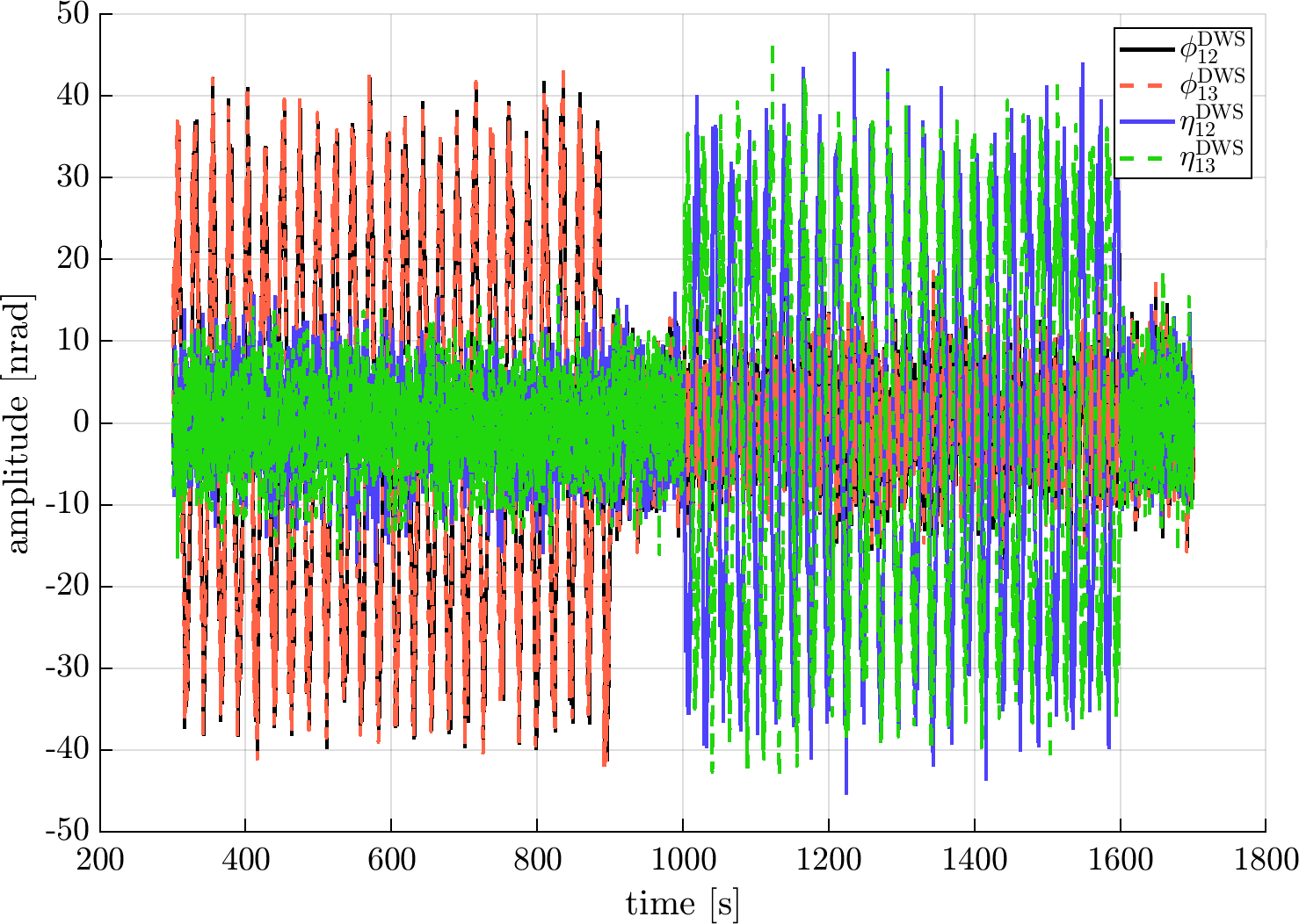
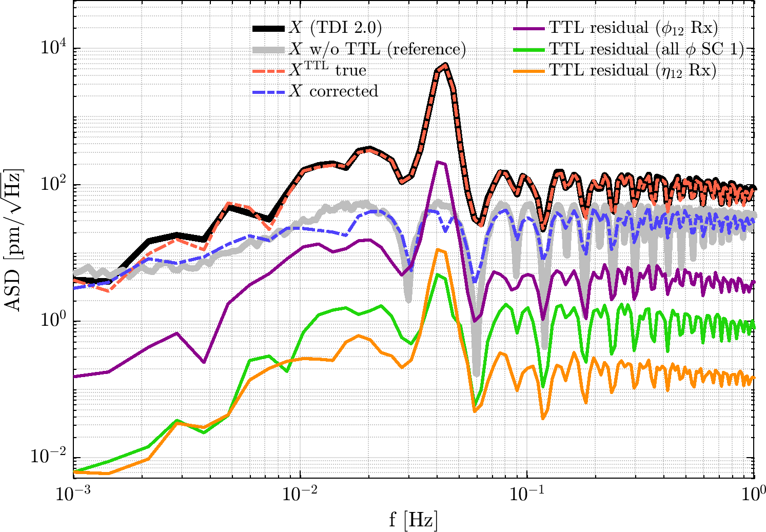
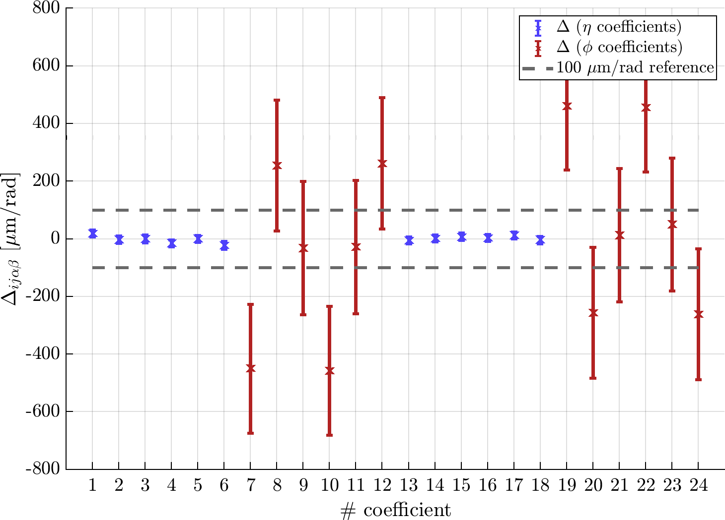
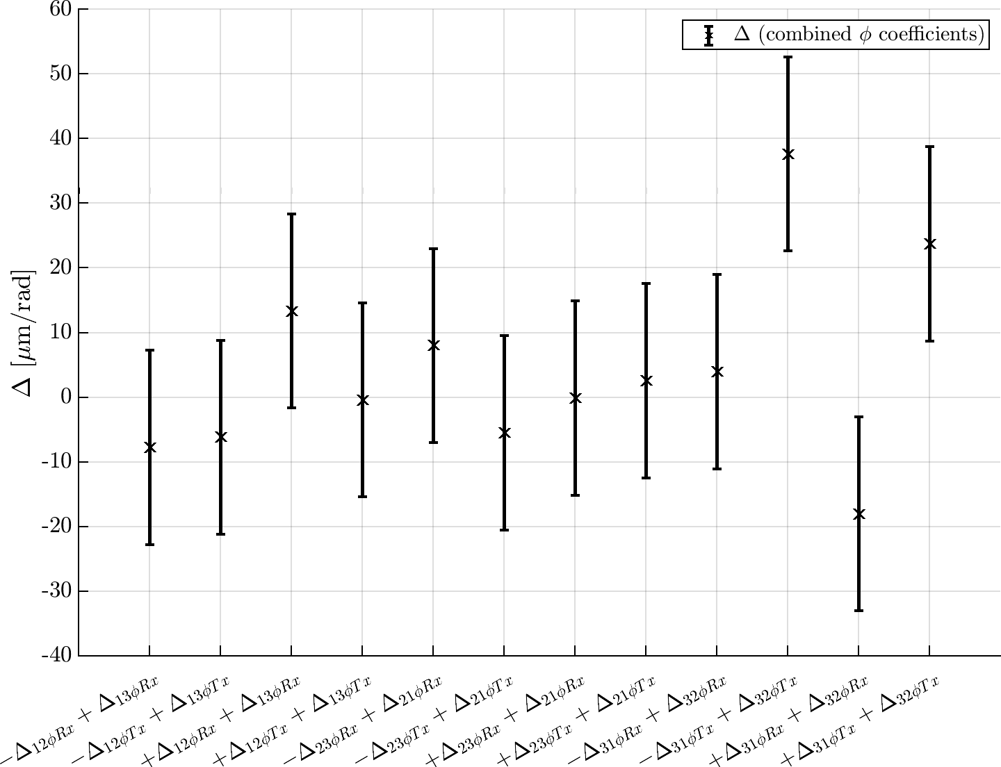
Figure 12: Simulation results for SC maneuvers. Top left: simulated DWS angles measured on SC $1$. Bottom left: ASD of $X$, $X^{\mathrm{TTL}}$ and different residuals, see explanation in the text. Top right: estimation errors $\Delta_{ij\alpha\beta}$. Bottom right: deviations of estimated combined $\phi$ coefficients.

Figure 12 shows some results of this simulation. The top left plot shows the simulated DWS measurements of both $\phi$ and $\eta$ angles on SC 1. The $\phi$ maneuvers take place from second $300$ to $900$, the $\eta$ maneuvers from second $1000$ to $1600$. For each SC, the excitations of the two MOSA $\eta$ angles have low correlation due to different frequencies, while the excitations of the two MOSA $\phi$ angles are highly correlated as explained in Sec. V.4. For this reason, the uncertainties of $\eta$ TTL coefficients are low, i.e. for coefficients # 1-6 (Rx) and 13-18 (Tx), and the uncertainties of the $\phi$ coefficients (# 7-12 and 19-24) are well above $0.1\text{\,}\mathrm{mm}\text{/}\mathrm{rad}$, the temporary requirement used e.g. in [6]. As illustrated in the top right plot, the actual deviations $\Delta_{ij\alpha\beta}=\hat{C}_{ij\alpha\beta}-C_{ij\alpha\beta}$ reflect these uncertainties, which are shown as error bars. This shows that $\phi$ maneuvers via SC rotation do not allow precise coefficient estimation. The Root Mean Square (RMS) deviation of the $\eta$ coefficients (# 1-6 and 13-18) was $10.6\text{\,}\mathrm{\SIUnitSymbolMicro m}\text{/}\mathrm{rad}$, for the individual $\phi$ coefficients (# 7-12 and 19-24) it was $303.4\text{\,}\mathrm{\SIUnitSymbolMicro m}\text{/}\mathrm{rad}$.

The deviations of the combined $\phi$ coefficients, however, were significantly lower than for the individual values. Estimated values for all $12$ such combinations are plotted in the bottom right of Fig. 12. For example, the deviations for SC $1$ were:

$$-\Delta_{12\phi Rx}+\Delta_{13\phi Rx} =$-7.7\text{\,}\mathrm{\SIUnitSymbolMicro m}\text{/}\mathrm{rad}$$$ (56)

$$-\Delta_{12\phi Tx}+\Delta_{13\phi Tx} =$-6.1\text{\,}\mathrm{\SIUnitSymbolMicro m}\text{/}\mathrm{rad}$$$ (57)

$$\Delta_{12\phi Rx}+\Delta_{12\phi Tx} =$13.4\text{\,}\mathrm{\SIUnitSymbolMicro m}\text{/}\mathrm{rad}$$$ (58)

$$\Delta_{13\phi Rx}+\Delta_{13\phi Tx} =$-0.3\text{\,}\mathrm{\SIUnitSymbolMicro m}\text{/}\mathrm{rad}$$$ (59)

Similar results were obtained for SC $2$ and SC $3$. The RMS deviation of all $12$ combined $\phi$ coefficients was $15.0\text{\,}\mathrm{\SIUnitSymbolMicro m}\text{/}\mathrm{rad}$, and therefore well below the temporary requirement of $100\text{\,}\mathrm{\SIUnitSymbolMicro m}\text{/}\mathrm{rad}$.

The bottom left plot of Fig. 12 shows several ASD, all of which stem from the SC maneuver simulation described in this subsection VI.3, except for the thick light gray line. The light gray line serves as a reference for $X$ without TTL and was obtained from a separate simulation with the coefficients set to zero. The TDI $X$ variable from the SC maneuver simulation is shown as a thick black line. It is dominated by the dashed red line, which shows the true total TTL computed with the true angles and the true coupling factors. The corrected $X$ variable (dashed blue line), i.e. $X-X^{\mathrm{TTL}}(\hat{C})$ computed with estimated coefficients and DWS angles, roughly coincides with the reference for $X$ without TTL, which shows that the subtraction of the estimated total TTL works. However, let us take a closer look at the residuals of the individual TTL contributions, i.e.

$$C_{ij\alpha\beta}\cdot\mathcal{X}_{ij\alpha\beta}-\hat{C}_{ij\alpha\beta}\cdot\mathcal{X}_{ij\alpha\beta}^{\mathrm{DWS}}.$$ (60)

It can bee seen that the residual for $X_{12\phi Rx}^{\mathrm{TTL}}$ alone (purple line) is much larger than for the sum of all $\phi$ TTL contributions for SC $1$ (green line). This is due to the large uncertainty of the individual estimated $\phi$ coefficients, but low uncertainty for the combined coefficients. For comparison, the dotted yellow line shows that the residual for $X_{12\eta Rx}^{\mathrm{TTL}}$ is much smaller than for $X_{12\phi Rx}^{\mathrm{TTL}}$ due to the low uncertainty of the $\eta$ coefficients. In summary, SC $\phi$ maneuvers can be used to subtract the combined TTL originating from $\phi$ angles, but do not allow precise estimation of the individual $\phi$ coefficients.

VI.4 Comparison of Estimation Uncertainties

We have compared our results to two other sources in the literature. Both sources assume the same linear TTL model for LISA and make statements about the uncertainty of the $24$ coefficients. In both cases, the angular jitter is modeled with ASD shapes similar to ours, cf. Fig. 4, merely with different jitter levels. The results are summarized in Tab. 7, where our values are given in terms of $\sigma_{\mathrm{stat}}=1.5\cdot\sigma_{\mathrm{LSQ}}$, cf. Sec. IV and App. B.

The first reference is [6], where the TTL coefficients are determined with an MCMC estimation in the frequency domain. For the main simulations, [6] used $2\text{\,}\mathrm{n}\mathrm{rad}\mathrm{/}\sqrt{\mathrm{Hz}}$ as the MOSA $\phi$ jitter level. However, a result is also given for $5\text{\,}\mathrm{n}\mathrm{rad}\mathrm{/}\sqrt{\mathrm{Hz}}$. We have performed two simulations in order to compare the results in both cases, either in terms of $\sigma(\hat{C}_{ij\alpha\beta})$ or in terms of RMS values, which are taken over the $24$ deviations $\hat{C}_{ij\alpha\beta}-C_{ij\alpha\beta}$. Here we find that we predict slightly lower uncertainties. Our computed standard deviations $\sigma_{\mathrm{stat}}$ are about a factor of $2$ smaller, cf. Tab. 7. A similar observation is made for the RMS values. Although the different estimation methods yield slightly different results, the overall picture of the feasibility of post-processing subtraction is still in agreement with our findings.

The second source we compared our results to is [8]. There, the authors obtain lower bounds for $\sigma(\hat{C})$ using Fisher information theory. We can compare to what is referred to as case A in [8], but not to the case B, where different jitter ASD shapes are used. Note also that this reference uses a slightly lower DWS noise level of $50/300$ $\mathrm{n}\mathrm{rad}\mathrm{/}\sqrt{\mathrm{Hz}}$. We have performed a simulation with the same settings given in [8] for case A. The lower bounds they obtain for the $\sigma(\hat{C}_{ij\alpha\beta})$ match well with our values for $\sigma_{\mathrm{stat}}$, cf. Tab. 7. This strengthens the confidence in our results and moreover suggests that the uncertainties we obtain are very close to optimal.

Table 7: Comparing coefficient uncertainties to results from two other sources in the literature, [6] and [8]. Based on simulated data with one day of integration time, without using maneuvers.

	jitter levels [$\mathrm{n}\mathrm{rad}\mathrm{/}\sqrt{\mathrm{Hz}}$]			uncertainty [$\mathrm{\SIUnitSymbolMicro m}\text{/}\mathrm{rad}$]		$\mathrm{n}\mathrm{rad}\mathrm{/}\sqrt{\mathrm{Hz}}$
Reference	SC (per axis)	MOSA $\eta$	MOSA $\phi$	$\sigma$	RMS	DWS noise level
source [6]	$5$	$1$	$2$	$23.7\leq\sigma\leq 38.6$	$\approx 35$	$70/335$
this study	$5$	$1$	$2$	$\sigma_{\mathrm{stat}}\approx(8.7,13.1)$	$12.6$	$70/335$
source [6]	$5$	$1$	$5$	N/A	$\approx 25$	$70/335$
this study	$5$	$1$	$5$	$\sigma_{\mathrm{stat}}\approx(8.7,6.3)$	$11.3$	$70/335$
- source [8]	$10$	$10$	$10$	$\sigma\geq(2.98,3.23)$	N/A	$50/300$
this study	$10$	$10$	$10$	$\sigma_{\mathrm{stat}}\approx(2.94,3.20)$	$2.6$	$50/300$

VII Summary and Outlook

In Sec. V, we discussed the feasibility and optimal design of TTL calibration maneuvers. We found that both SC and MOSA maneuvers are likely possible with amplitudes of about $30\text{\,}\mathrm{nrad}\text{/}$. The optimal frequency for periodic injection signals is $43$ (40-45) $\mathrm{mHz}\text{/}$, or, alternatively, about $18$ or $78$ mHz. Uncorrelated pairs can be used to perform maneuvers partly simultaneously. Using these pairs and three different frequencies allows to perform two sets of six simultaneous maneuvers each, covering all $12$ angles which cause TTL. Since Rx and Tx coefficients can also be estimated at the same time, this is sufficient to recover all $24$ TTL coefficients. While $\eta$ maneuvers can be performed via injection into SC angles, $\phi$ maneuvers should be done via MOSA injections if one wants to disentangle the individual $\phi$ coefficients. Alternatively, three SC $\phi$ maneuvers allow to estimate combined $\phi$ coefficients, which is sufficient for TTL subtraction, as we confirmed in Sec. VI.3.

In Sec. VI, we have shown that with a total maneuver duration of $20$ minutes, all TTL coupling coefficients could be recovered with uncertainties below $15\text{\,}\mathrm{\SIUnitSymbolMicro m}\text{/}\mathrm{rad}$, which is more than sufficient for TTL subtraction. When comparing the estimation using maneuvers to a fit-of-noise approach, the improvement factor in terms of integration time required to achieve this uncertainty level was about $9$ in the case of full angular jitter. In the alternative scenario with the reduced MOSA $\phi$ jitter level of $0.5\text{\,}\mathrm{n}\mathrm{rad}\mathrm{/}\sqrt{\mathrm{Hz}}$, maneuvers would even reduce the required integration time by a factor of about $230$. This shows that maneuvers can be used to determine the TTL coefficients significantly quicker. However, whether the potential improvement justifies performing maneuvers will likely depend on the MOSA $\phi$ jitter level and frequency shape in a closed-loop control system. Finally, we found that the estimation uncertainties obtained from our simulations are compatible with results from [6] and [8].

This document provides a first-level assessment of the feasibility of TTL calibration maneuvers in LISA, and of the potential improvement for coefficient estimation. For concrete planning, the actual realization of the maneuvers should be studied in more detail.

Appendix A TTL Contributions in the TDI Variables

We are working with the TDI 2.0 variables [2, 13, 12]. The second generation Michelson combination $X$ is shown in equation $(4.33)$ in [12]. From this, one can derive the formula for all TTL in $X$ due to $\eta$ angles:

$$X^{\mathrm{TTL}}_{\eta}=- \left(1-\mathcal{D}_{131}-\mathcal{D}_{13121}+\mathcal{D}_{1213131}\right)\left((C_{12\eta Rx}+C_{12\eta Tx}\mathcal{D}_{121})\eta_{12}+(C_{21\eta Rx}+C_{21\eta Tx})\mathcal{D}_{12}\eta_{21}\right)$$

$$+ \left(1-\mathcal{D}_{121}-\mathcal{D}_{12131}+\mathcal{D}_{1312121}\right)\left((C_{13\eta Rx}+C_{13\eta Tx}\mathcal{D}_{131})\eta_{13}+(C_{31\eta Rx}+C_{31\eta Tx})\mathcal{D}_{13}\eta_{31}\right).$$ (61)

Note that the signs in Eq. (61) are conventional and may be swapped in other publications. Replacing all $\eta$’s with $\phi$’s yields the TTL in $X$ due to the $\phi$ angles, $X^{\mathrm{TTL}}_{\phi}$, and the entire TTL in $X$ is given by the sum $X^{\mathrm{TTL}}=X^{\mathrm{TTL}}_{\eta}+X^{\mathrm{TTL}}_{\phi}$. The combinations $Y$ and $Z$ are obtained by circular permutation of the indices. Here $\phi_{ij}$ and $\eta_{ij}$ denote the pitch and yaw angles of MOSA $ij$ w.r.t. incident beam originating from SC $j$, cf. Sec.II.1. We contracted the indices according to the convention given in Sec. II.2. For reference, we write out the individual equations for all TTL contributions depending on $\eta$ angles in the following. The TTL contributions of the $\phi$ angles are built identically, i.e. they can be obtained by replacing each $\eta$ with a $\phi$.

For $\eta_{12}$ Rx (coefficient #1, using the numbering convention given in Tab. 1) we have:

$$X_{12\eta Rx}^{\mathrm{TTL}}= C_{12\eta Rx}\cdot(-1+\mathcal{D}_{131}+\mathcal{D}_{13121}-\mathcal{D}_{1213131})\eta_{12}$$ (62)

$$Y_{12\eta Rx}^{\mathrm{TTL}}= C_{12\eta Rx}\cdot(1-\mathcal{D}_{232}-\mathcal{D}_{23212}+\mathcal{D}_{2123232})\mathcal{D}_{21}\eta_{12}$$ (63)

$$Z_{12\eta Rx}^{\mathrm{TTL}}= 0$$ (64)

For $\eta_{12}$ Tx (#13) we have:

$$X_{12\eta Tx}^{\mathrm{TTL}} =C_{12\eta Tx}\cdot(-1+\mathcal{D}_{131}+\mathcal{D}_{13121}-\mathcal{D}_{1213131})\mathcal{D}_{121}\eta_{12}$$ (65)

$$Y_{12\eta Tx}^{\mathrm{TTL}} =C_{12\eta Tx}\cdot(1-\mathcal{D}_{232}-\mathcal{D}_{23212}+\mathcal{D}_{2123232})\mathcal{D}_{21}\eta_{12}$$ (66)

$$Z_{12\eta Tx}^{\mathrm{TTL}} =0$$ (67)

For $\eta_{23}$ Rx (#2) we have:

$$X_{23\eta Rx}^{\mathrm{TTL}} =0$$ (68)

$$Y_{23\eta Rx}^{\mathrm{TTL}} =C_{23\eta Rx}\cdot(-1+\mathcal{D}_{212}+\mathcal{D}_{21232}-\mathcal{D}_{2321212})\eta_{23}$$ (69)

$$Z_{23\eta Rx}^{\mathrm{TTL}} =C_{23\eta Rx}\cdot(1-\mathcal{D}_{313}-\mathcal{D}_{31323}+\mathcal{D}_{3231313})\mathcal{D}_{32}\eta_{23}$$ (70)

For $\eta_{23}$ Tx (#14) we have:

$$X_{23\eta Tx}^{\mathrm{TTL}} =0$$ (71)

$$Y_{23\eta Tx}^{\mathrm{TTL}} =C_{23\eta Tx}\cdot(-1+\mathcal{D}_{212}+\mathcal{D}_{21232}-\mathcal{D}_{2321212})\mathcal{D}_{232}\eta_{23}$$ (72)

$$Z_{23\eta Tx}^{\mathrm{TTL}} =C_{23\eta Tx}\cdot(1-\mathcal{D}_{313}-\mathcal{D}_{31323}+\mathcal{D}_{3231313})\mathcal{D}_{32}\eta_{23}$$ (73)

For $\eta_{31}$ Rx (#3) we have:

$$X_{31\eta Rx}^{\mathrm{TTL}} =C_{31\eta Rx}\cdot(1-\mathcal{D}_{121}-\mathcal{D}_{12131}+\mathcal{D}_{1312121})\mathcal{D}_{13}\eta_{31}$$ (74)

$$Y_{31\eta Rx}^{\mathrm{TTL}} =0$$ (75)

$$Z_{31\eta Rx}^{\mathrm{TTL}} =C_{31\eta Rx}\cdot(-1+\mathcal{D}_{323}+\mathcal{D}_{32313}-\mathcal{D}_{3132323})\eta_{31}$$ (76)

For $\eta_{31}$ Tx (#15) we have:

$$X_{31\eta Tx}^{\mathrm{TTL}} =C_{31\eta Tx}\cdot(1-\mathcal{D}_{121}-\mathcal{D}_{12131}+\mathcal{D}_{1312121})\mathcal{D}_{13}\eta_{31}$$ (77)

$$Y_{31\eta Tx}^{\mathrm{TTL}} =0$$ (78)

$$Z_{31\eta Tx}^{\mathrm{TTL}} =C_{31\eta Tx}\cdot(-1+\mathcal{D}_{323}+\mathcal{D}_{32313}-\mathcal{D}_{3132323})\mathcal{D}_{313}\eta_{31}$$ (79)

For $\eta_{13}$ Rx (#4) we have:

$$X_{13\eta Rx}^{\mathrm{TTL}} =C_{13\eta Rx}\cdot(1-\mathcal{D}_{121}-\mathcal{D}_{12131}+\mathcal{D}_{1312121})\eta_{13}$$ (80)

$$Y_{13\eta Rx}^{\mathrm{TTL}} =0$$ (81)

$$Z_{13\eta Rx}^{\mathrm{TTL}} =C_{13\eta Rx}\cdot(-1+\mathcal{D}_{323}+\mathcal{D}_{32313}-\mathcal{D}_{3132323})\mathcal{D}_{31}\eta_{13}$$ (82)

For $\eta_{13}$ Tx (#16) we have:

$$X_{13\eta Tx}^{\mathrm{TTL}} =C_{13\eta Tx}\cdot(1-\mathcal{D}_{121}-\mathcal{D}_{12131}+\mathcal{D}_{1312121})\mathcal{D}_{131}\eta_{13}$$ (83)

$$Y_{13\eta Tx}^{\mathrm{TTL}} =0$$ (84)

$$Z_{13\eta Tx}^{\mathrm{TTL}} =C_{13\eta Tx}\cdot(-1+\mathcal{D}_{323}+\mathcal{D}_{32313}-\mathcal{D}_{3132323})\mathcal{D}_{31}\eta_{13}$$ (85)

For $\eta_{32}$ Rx (#5) we have:

$$X_{32\eta Rx}^{\mathrm{TTL}} =0$$ (86)

$$Y_{32\eta Rx}^{\mathrm{TTL}} =C_{32\eta Rx}\cdot(-1+\mathcal{D}_{212}+\mathcal{D}_{21232}-\mathcal{D}_{2321212})\mathcal{D}_{23}\eta_{32}$$ (87)

$$Z_{32\eta Rx}^{\mathrm{TTL}} =C_{32\eta Rx}\cdot(1-\mathcal{D}_{313}-\mathcal{D}_{31323}+\mathcal{D}_{3231313})\eta_{32}$$ (88)

For $\eta_{32}$ Tx (#17) we have:

$$X_{32\eta Tx}^{\mathrm{TTL}} =0$$ (89)

$$Y_{32\eta Tx}^{\mathrm{TTL}} =C_{32\eta Tx}\cdot(-1+\mathcal{D}_{212}+\mathcal{D}_{21232}-\mathcal{D}_{2321212})\mathcal{D}_{23}\eta_{32}$$ (90)

$$Z_{32\eta Tx}^{\mathrm{TTL}} =C_{32\eta Tx}\cdot(1-\mathcal{D}_{313}-\mathcal{D}_{31323}+\mathcal{D}_{3231313})\mathcal{D}_{323}\eta_{32}$$ (91)

For $\eta_{21}$ Rx (#6) we have:

$$X_{21\eta Rx}^{\mathrm{TTL}} =C_{21\eta Rx}\cdot(-1+\mathcal{D}_{131}+\mathcal{D}_{13121}-\mathcal{D}_{1213131})\mathcal{D}_{12}\eta_{21}$$ (92)

$$Y_{21\eta Rx}^{\mathrm{TTL}} =C_{21\eta Rx}\cdot(1-\mathcal{D}_{232}-\mathcal{D}_{23212}+\mathcal{D}_{2123232})\eta_{21}$$ (93)

$$Z_{21\eta Rx}^{\mathrm{TTL}} =0$$ (94)

For $\eta_{21}$ Tx (#18) we have:

$$X_{21\eta Tx}^{\mathrm{TTL}} =C_{21\eta Tx}\cdot(-1+\mathcal{D}_{131}+\mathcal{D}_{13121}-\mathcal{D}_{1213131})\mathcal{D}_{12}\eta_{21}$$ (95)

$$Y_{21\eta Tx}^{\mathrm{TTL}} =C_{21\eta Tx}\cdot(1-\mathcal{D}_{232}-\mathcal{D}_{23212}+\mathcal{D}_{2123232})\mathcal{D}_{212}\eta_{21}$$ (96)

$$Z_{21\eta Tx}^{\mathrm{TTL}} =0$$ (97)

Appendix B Statistical estimator uncertainty

In order to gain a better understanding of realistic uncertainties, we performed a test by simulating $500$ sets of LISA data, each of length $2000\text{\,}\mathrm{s}\text{/}$ and with identical noise settings as specified in Tab. 3. In each simulation, different random coefficients were used, uniformly distributed within the interval $[-3,3]$ $\mathrm{mm}\text{/}\mathrm{rad}$. For each coefficient $C_{ij\alpha\beta}$ we computed the standard deviation of all deviations $\Delta_{ij\alpha\beta}=\hat{C}_{ij\alpha\beta}-C_{ij\alpha\beta}$ over $500$ runs. These statistical standard deviations were within $[61.5,68]$ $\mathrm{\SIUnitSymbolMicro m}\text{/}\mathrm{rad}$ for the $\eta$ coefficients and within $[45.5,49]$ $\mathrm{\SIUnitSymbolMicro m}\text{/}\mathrm{rad}$ for $\phi$, while the standard deviations obtained by formula (25) were within $[42.8,47.8]$ $\mathrm{\SIUnitSymbolMicro m}\text{/}\mathrm{rad}$ for $\eta$ and within $[31.4,35]$ $\mathrm{\SIUnitSymbolMicro m}\text{/}\mathrm{rad}$ for $\phi$. For each coefficient, the ratio of statistical standard deviations over $\sigma_{\mathrm{LSQ}}$ was between $1.4$ and $1.5$. We conclude that a more realistic uncertainty is given by the value $\sigma_{\mathrm{stat}}$, which we define as

$$\sigma_{\mathrm{stat}}=1.5\cdot\sigma_{\mathrm{LSQ}}.$$ (98)

Appendix C Dependencies of LSQ estimator uncertainty

Suppose we estimate merely two of the TTL coefficients and denote these by $C_{1},C_{2}$. We can use the same notation as described in Sec. II, just considering two instead of all $24$ TTL contributions. That is, we define $\mathcal{A}=[\mathcal{A}_{1},\mathcal{A}_{2}]\in\mathbb{R}^{3N\times 2}$ as in Eq.(15), but taking only the two relevant columns. The sum of these two TTL contributions in $V=(X^{T},Y^{T},Z^{T})^{T}$ is given by $\mathcal{A}\cdot C$, with $C=[C_{1},C_{2}]^{T}$, just as in Eq.(18). Assume further without loss of generality that each column of $\mathcal{A}$ has zero mean. Recall that the formal error of the LSQ estimator is given in Eq. (25). If we define $M:=(\mathcal{A}^{T}\mathcal{A})^{-1}$, with $M_{11}$ denoting the top left matrix entry, we have

$$\sigma_{\mathrm{LSQ}}(\hat{C}_{1})=\sigma(n_{V})\cdot\sqrt{M_{11}}\propto\sqrt{M_{11}}$$ (99)

where $\hat{C}_{1}$ is the LSQ estimator of $C_{1}$. Since $\mathcal{A}^{T}\mathcal{A}$ is a $2\times 2$ matrix, its inverse $M$ is given by an explicit formula. In particular,

$$M_{11}=\frac{1}{\det(\mathcal{A}^{T}\mathcal{A})}\mathcal{A}_{2}^{T}\mathcal{A}_{2}$$ (100)

with

$$\det(\mathcal{A}^{T}\mathcal{A})=(\mathcal{A}_{1}^{T}\mathcal{A}_{1})(\mathcal{A}_{2}^{T}\mathcal{A}_{2})-(\mathcal{A}_{1}^{T}\mathcal{A}_{2})^{2}.$$ (101)

Equation (100) can be written in terms of the standard deviation $\sigma(\mathcal{A}_{1})$ and the correlation $\mathrm{corr}(\mathcal{A}_{1},\mathcal{A}_{2})$. In our matrix notation these can be expressed as

$$\sigma(\mathcal{A}_{i})^{2}=\frac{1}{3N}\mathcal{A}_{i}^{T}\mathcal{A}_{i},$$ (102)

$i=1,2$, and

$$\mathrm{corr}(\mathcal{A}_{1},\mathcal{A}_{2}) =\frac{\mathrm{cov}(\mathcal{A}_{1},\mathcal{A}_{2})}{\sigma(\mathcal{A}_{1})\sigma(\mathcal{A}_{2})}$$ (103)

$$=\frac{\mathcal{A}_{1}^{T}\mathcal{A}_{2}}{\sqrt{(\mathcal{A}_{1}^{T}\mathcal{A}_{1})(\mathcal{A}_{2}^{T}\mathcal{A}_{2})}},$$ (104)

provided that each $\mathcal{A}_{i}$ has zero mean. Now, rearranging the terms of Eq. (100) yields

$$M_{11} =\frac{\mathcal{A}_{2}^{T}\mathcal{A}_{2}}{(\mathcal{A}_{1}^{T}\mathcal{A}_{1})(\mathcal{A}_{2}^{T}\mathcal{A}_{2})-(\mathcal{A}_{1}^{T}\mathcal{A}_{2})^{2}}$$ (105)

$$=\frac{\mathcal{A}_{2}^{T}\mathcal{A}_{2}}{(\mathcal{A}_{1}^{T}\mathcal{A}_{1})(\mathcal{A}_{2}^{T}\mathcal{A}_{2})(1-\mathrm{corr}(\mathcal{A}_{1},\mathcal{A}_{2})^{2})}$$ (106)

$$=\frac{1}{3N\cdot\sigma(\mathcal{A}_{1})^{2}\cdot(1-\mathrm{corr}(\mathcal{A}_{1},\mathcal{A}_{2})^{2})},$$ (107)

provided $\mathrm{corr}(\mathcal{A}_{1},\mathcal{A}_{2})^{2}\neq 1$ since otherwise the two columns of $\mathcal{A}$ are linearly dependent and $M$ does not exist to start with. Hence it follows that

$$\sigma_{\mathrm{LSQ}}(\hat{C}_{1})\propto\frac{1}{\sqrt{N}}\frac{1}{\sigma(\mathcal{A}_{1})}\frac{1}{\sqrt{1-\mathrm{corr}(\mathcal{A}_{1},\mathcal{A}_{2})^{2}}}.$$ (108)

In particular, if $\mathcal{A}_{1}$ is dominated by a sinusoidal injection angle with amplitude $A_{\mathrm{man}}$, then $\mathcal{A}_{1}$ is approximately proportional to $A_{\mathrm{man}}$ as well, and we clearly have

$$\sigma_{\mathrm{LSQ}}(\hat{C}_{1})\propto\frac{1}{A_{\mathrm{man}}}$$ (109)

for large enough $A_{\mathrm{man}}$. Moreover, for the maneuver duration $T_{\mathrm{man}}$ we then have

$$\sigma_{\mathrm{LSQ}}(\hat{C}_{1})\propto\frac{1}{\sqrt{T_{\mathrm{man}}}}$$ (110)

since $N\propto T_{\mathrm{man}}$ for a fixed sampling rate, where $T_{\mathrm{man}}$ is the maneuver time that is used entirely for the estimation. Note that this dependency requires the noise $n_{V}$ in the TDI variables to be white, which the LSQ estimator does assume. In reality the noise spectrum is frequency dependent and it is clear that the estimation uncertainty cannot be lowered arbitrarily by increasing the amount of sampling points $N$.

Since the two TTL contributions were chosen arbitrarily in the beginning, the result holds for any two TTL contributions, if only these two are estimated and there are no correlations with other contributions. When all $24$ TTL coefficients are estimated at the same time, the relations 109 and 110 still hold approximately. We have confirmed this with simulations. The results for the coefficient $C_{12\eta Rx}$ are shown in Fig. 13. For the left plot, $100$ simulations were performed, each including an $\eta_{12}$ maneuver with an amplitude between $0$ and $200\text{\,}\mathrm{nrad}\text{/}$, while all other settings were fixed. The maneuver duration was fixed to $T_{\mathrm{man}}~{}=$ $2000\text{\,}\mathrm{s}\text{/}$, the maneuver frequency was $f_{\mathrm{man}}~{}=$ $43\text{\,}\mathrm{mHz}\text{/}$. Shown in blue are $\sigma_{\mathrm{LSQ}}(\hat{C}_{12\eta Rx})$, plotted over $A_{\mathrm{man}}$. The red dashed line shows the predicted values, which were obtained by extrapolating an example value according to the relation 109. For significant amplitudes $>$ $20\text{\,}\mathrm{nrad}\text{/}$, when the TTL contribution of $\eta_{12}$ is dominated by the maneuver signal, the standard deviations from the simulations are compatible with the predicted values, confirming proportionality $\sigma\propto 1/A_{\mathrm{man}}$.

The right plot of Fig. 13 shows again $100$ different values of $\sigma(\hat{C}_{12\eta Rx})$ in blue. A long $\eta_{12}$ maneuver with a duration of $10\,000\text{\,}\mathrm{s}\text{/}$ was simulated. The maneuver amplitude was $100\text{\,}\mathrm{nrad}\text{/}$, the maneuver frequency was $f_{\mathrm{man}}=$ $43\text{\,}\mathrm{mHz}\text{/}$. For each of the $100$ plotted values, a different data length was used for the estimation and computation of the standard deviation. The red dashed line shows the predicted standard deviations, according to relation 110, plotted over $T_{\mathrm{man}}$. In particular, the plot confirms the proportionality $\sigma\propto 1/\sqrt{T_{\mathrm{man}}}$.

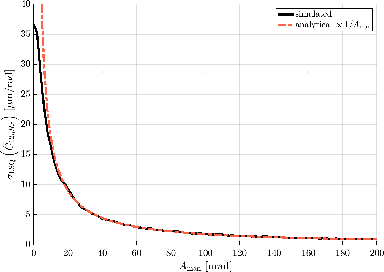
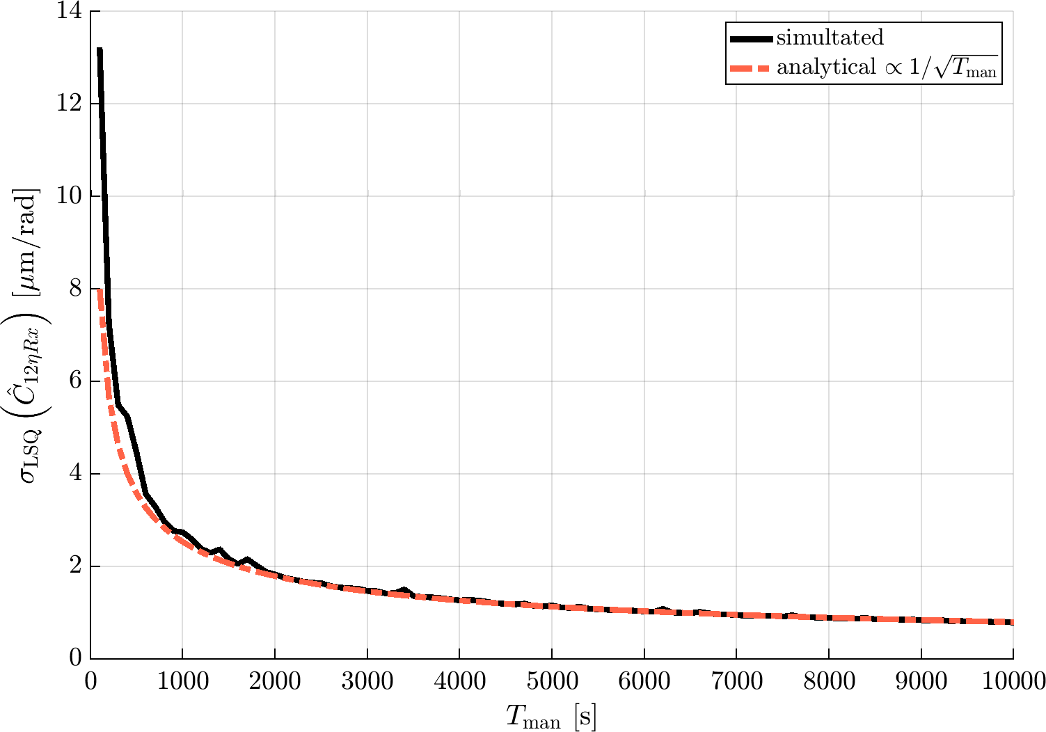
Figure 13: Dependency of estimator uncertainties to $1/A_{\mathrm{man}}$ (left) and $1/\sqrt{T_{\mathrm{man}}}$ (right), confirmed with simulations.

Recall that, for SC maneuvers, the maneuver amplitude may be limited by the maximally achievable torque, which we did not assume. Should that be the case, we have furthermore

$$A_{\mathrm{man}}\propto\frac{1}{f_{\mathrm{man}}^{2}},$$ (111)

and hence

$$\sigma\propto\frac{f_{\mathrm{man}}^{2}}{\sqrt{T_{\mathrm{man}}}}.$$ (112)