Repurposing Stable Diffusion Attention for Training-Free Unsupervised Interactive Segmentation

Abstract

Recent progress in interactive point prompt based Image Segmentation allows to significantly reduce the manual effort to obtain high quality semantic labels. State-of-the-art unsupervised methods use self-supervised pre-trained models to obtain pseudo-labels which are used in training a prompt-based segmentation model. In this paper, we propose a novel unsupervised and training-free approach based solely on the self-attention of Stable Diffusion. We interpret the self-attention tensor as a Markov transition operator, which enables us to iteratively construct a Markov chain. Pixel-wise counting of the required number of iterations along the Markov chain to reach a relative probability threshold yields a Markov-iteration-map, which we simply call a Markov-map. Compared to the raw attention maps, we show that our proposed Markov-map has less noise, sharper semantic boundaries and more uniform values within semantically similar regions. We integrate the Markov-map in a simple yet effective truncated nearest neighbor framework to obtain interactive point prompt based segmentation. Despite being training-free, we experimentally show that our approach yields excellent results in terms of Number of Clicks (NoC), even outperforming state-of-the-art training based unsupervised methods in most of the datasets.

1 Introduction

The goal of point prompt based interactive image segmentation is to obtain a high-quality segmentation from limited user interaction in the form of clicking. Prompt based image segmentation gained popularity lately due to large supervised foundation models [15, 28]. In this paper, we focus on unsupervised methods, where no segmentation labels are used at all in the design and/or training of the models. Most recent approaches rely on self supervised backbones like ViT [6], trained either by DINO [2] or MAE [12] based self-supervised techniques. On the other hand, Stable Diffusion (SD) [29] has been used for many different computer vision applications such as monocular depth estimation [14], semantic segmentation [38], object detection [3] and image classification [17], often resulting in state-of-the-art solutions.

Inspired by DiffSeg [38], we utilize SD’s self-attention maps in our training-free interactive segmentation approach. The main challenges are that attention maps are noisy and don’t distinguish between instances. To overcome the mentioned challenges, we interpret the self-attention tensors as a Markov transition operator, where the repeated application of the transition forms a Markov chain. We propose a novel Markov-iteration-map or simply Markov-map, where each pixel counts the number of iterations required to obtain a specific probability value. We show that the proposed Markov-map has less noise, the semantic boundaries are sharper and the semantic regions within Markov-maps are more uniformly distributed. Native Markov-maps do not distinguish between instances. Therefore, we further improve Markov-maps with a flood fill approach, which suppresses local minima, to enable instance based segmentation. Finally, we obtain Markov-maps of each prompt point and combine them with a truncated nearest neighbor approach to enable multi-prompt point interactive segmentation. Surprisingly, despite being training-free, we significantly improve the state-of-the-art in terms of Number of Clicks (NoC) and even surpass training based unsupervised approaches in most of the datasets. Our main contributions are:

• We introduce Markov-Map Nearest Neighbor (M2N2), the first attention-based unsupervised training-free multi-point prompt segmentation framework.

• We propose Markov-maps in order to improve the semantic information.

• We enable instance aware Markov-maps by utilizing a modified flood fill approach.

• We introduce a truncated nearest neighbor approach to combine multiple point prompts.

• We conduct extensive experiments and achieve state-of-the-art results, surpassing even unsupervised training-based methods.

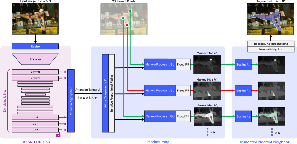
Figure 1: M2N2 framework overview. We perform a single denoising step of the input image with Stable Diffusion 2 to obtain attention tensors. The tensors are aggregated and utilized to obtain a Markov-map $M_{i}$ for each prompt point. The final segmentation is the result of a truncated nearest neighbor of scaled Markov-maps $M_{i}$ as a measure of semantic distance for each prompt point. The green and red areas in the scaled Markov-maps denote regions where the distance is less or equal to the global background threshold. In this visualization, components in blue contain adjustable hyperparameters.

2 Related Work

Point prompt based interactive image segmentation has been approached from multiple perspectives. In this paper, we distinguish between supervised and unsupervised methods.

2.1 Supervised Methods

In [44] a click map and click sampling strategies are used in combination with FCN [24], creating the foundation for many follow-up methods.

In [20] the first click is emphasized, while in [13, 35], backpropagation refinement schemes (BRS) are proposed as a refinement step to correct mislabeled pixels. Diffusing prediction is introduced in [4], which propagates labeled representations from clicks to conditioned destinations and in [10], where interactive information of user clicks with edge-guided flow is utilized. Iterative click sampling [36] proposes a simple feed-forward model for click-based interactive segmentation that employs the segmentation masks from previous steps. SimpleClick [23] utilizes ViT, pre-trained as a masked autoencoder (MAE), for feature generation. Gaussian process posterior [46] formulates the Image Segmentation task as a Gaussian process-based pixel-wise binary classification model to fully and explicitly utilize and propagate the click information. In [21, 5] the authors propose to segment on local crops to improve efficiency. In [22] click prompt learning with Optimal Transport is proposed, which leverages optimal transport theory to capture diverse user intentions with multiple click prompts. CFR-ICL [37] introduces three components to improve the interactive segmentation, namely Cascade-Forward Refinement, Iterative Click Loss and diverse augmentation, respectively.

Although the supervised approaches achieve good performance and efficiency, they require large-scale pixel-level annotations to train, which are expensive and laborious to obtain. While many supervised methods are tested on additional domains like medical images, it is unclear if there are other domains where the trained models would have a domain gap.

2.2 Unsupervised methods

Classical, unsupervised methods not based on Deep Learning like GraphCut [31], Random Walk [7], Geodesic Matting [1], GSC [8] and ESC [8] have been proposed. However, recently Deep Learning based approaches show great potential. Especially, methods utilizing self-supervised learning achieve impressive results. Such methods rely on pre-trained models (e.g., DenseCL [39], DINO [2]) to extract segments from their features. In [33] some heuristics are proposed to choose pixels belonging to the same object according to their feature similarity. [42] introduces normalized cuts [32] on the affinity graph constructed by pixel-level representations from DINO to divide the foreground and background of an image. In [9] a segmentation head is trained by distilling the feature correspondences from DINO. [26] adopts spectral decomposition on the affinity graph to discover meaningful parts in an image. FreeSOLO [40] designs pseudo instance mask generation based on multi-scale feature correspondences from densely pre-trained models and trains an instance segmentation model with these pseudo masks.
Recently, several papers used Stable Diffusion (SD) [29] for various kinds of applications targeting unsupervised Semantic Segmentation. In [38] the self-attention maps of SD were used with KL-Divergence based similarity measures to merge semantically similar regions in order to extract segments. MIS [18] and UnSAM [41] use methods to capture the semantic hierarchy and create pseudo labels, which are used in a follow-up training process to obtain a model for promptable segmentation. UnSAM additionally allows automatic whole-image segmentation, but does not report NoC values on any dataset. In [3] object detection is formulated as a denoising diffusion process from noisy boxes to object boxes, and [19] proposes training-free unsupervised segmentation using a pre-trained diffusion model by iteratively contrasting the original image and a painted image in which a masked area is re-painted. While this method obtains good results, it does not provide multi-prompt interactive segmentation.

Inspired by [38], we focus on SD’s self-attention maps as an initial semantic feature map. Our proposed Markov-map improves the semantic features, resulting in an excellent, unsupervised point prompt based interactive segmentation solution.

3 Method

In this section, we introduce our Markov-Map Nearest Neighbor (M2N2) framework in full detail. As shown in Fig. 1, M2N2 is composed of three main stages. In the first stage, we obtain an attention tensor of the input image by aggregating SD’s self-attentions. The second stage extracts and enhances the semantic information of the attention tensor by creating a Markov-map for each prompt point. The semantically rich Markov-maps are then utilized in a truncated nearest neighbor algorithm to obtain a training-free unsupervised segmentation.

In the following subsections, we first formulate the problem in the context of a nearest neighbor algorithm in Sec. 3.1, followed by an explanation of the acquisition of the attention tensor in Sec. 3.2 and extraction of the Markov-maps including the flood fill approach in Sec. 3.3. Finally, we introduce the full M2N2 algorithm Sec. 3.4.

3.1 Truncated Nearest Neighbor

In point prompt based segmentation we are given an image $I\in\mathbb{R}^{H\times W\times 3}$ of width $W$ and height $H$ and a set of labeled prompt points $D=\{(x_{1},y_{1}),(x_{2},y_{2}),...,(x_{N},y_{N})\}$ where $x_{i}\in\mathbb{R}^{2}$ are the 2D spatial coordinates of each prompt point in image pixel space and the labels $y_{i}\in\{0,1\}$ denote whether a point $x_{i}$ belongs to the background $y_{i}=0$ or foreground $y_{i}=1$. To perform k-NN segmentation with $k=1$, we assign each query pixel $x_{q}$ of our output segmentation the class of its nearest neighbor $x_{i^{*}}$:

$$i^{*}=\underset{i}{\arg\min}~{}d(x_{i},x_{q}),\;\;\;\;\;\;\;\;y_{q}=y_{i^{*}}$$ (1)

where $d(\cdot,\cdot):\mathbb{R}^{2}\times\mathbb{R}^{2}\rightarrow\mathbb{R}_{\geq 0}$ is a semantic distance function measuring the semantic similarity between the query pixel $x_{q}$ and prompt point $x_{i}$. In our case, we allow $d(\cdot,\cdot)$ to be asymmetric, meaning that $d(x_{i},x_{q})$ may, but does not have to, equal $d(x_{q},x_{i})$. Using a canonical 1-NN, a single foreground prompt point would always segment the entire image as foreground, requiring a minimum of two prompts, one foreground and one background prompt, to get a useful segmentation. To mitigate this limitation and reduce NoC, we further extend the 1-NN algorithm with a distance threshold of $1$ and define $\hat{y}_{q}$ as:

$$\hat{y}_{q}=\begin{cases}y_{i^{*}}&\text{if }d(x_{i^{*}},x_{q})\leq 1\\ 0&\text{otherwise.}\end{cases}$$ (2)

If the distance between a query pixel $x_{q}$ and its nearest neighbor $x_{i^{*}}$ exceeds the threshold of $1$, it is classified as background $\hat{y}_{q}=0$, independent of its nearest neighbor’s class $y_{i^{*}}$. The main challenge is to find a good distance function $d(\cdot,\cdot)$ which measures the semantic dissimilarity of a prompt point $x_{i}$ and a query pixel $x_{q}$.

3.2 Attention Aggregation

In this paper, we use the pre-trained SD 2. Given an image $I$, we perform a single denoising step by computing a forward pass through the denoising U-Net and extract the multi-head self-attentions $\boldsymbol{S}_{j}$ of each transformer block $j$. Each tensor $\boldsymbol{S}_{j}$ is of the shape $N_{heads}\times h\times w\times h\times w$. $N_{heads}$ denotes the number of attention heads and $h$ and $w$ are the height and width of the attention maps respectively. Each attention map $\boldsymbol{S}_{j}[n,k,l,:,:]$ of the tensor $\boldsymbol{S}_{j}$ is a probability distribution, meaning the sum of each map’s elements is equal to $1$. We define the aggregated tensor $\boldsymbol{A}\in\mathbb{R}^{h\times w\times h\times w}$ as follows:

$$\boldsymbol{A}[:,:,:,:] =\sum_{j\in\mathrm{AttnBlocks}}w_{j}\sum_{n}^{N_{heads}}\boldsymbol{S}_{j}[n,:,:,:,:]$$ (3)

Ensuring that the sum of weights $w_{j}\in[0,1]$ is $1$, the result is a single attention tensor $\boldsymbol{A}$ of which each 2D-map $\boldsymbol{A}[k,l,:,:]$ is a probability distribution.

3.3 From Attention Tensor to Markov-Maps

First, we flatten the attention tensor $\boldsymbol{A}\in\mathbb{R}^{h\times w\times h\times w}$ to obtain a matrix $A\in\mathbb{R}^{(h\cdot w)\times(h\cdot w)}$. Since $A$ is a right stochastic matrix, we can use it as a transition matrix in a Markov chain:

$$p_{t}=p_{0}\cdot A^{t}\;\;\;\;\mathrm{with}\;\;\;\;p_{0}=onehot(x)$$ (4)

where the probability distribution row vector $p_{0}\in\mathbb{R}^{1\times(h\cdot w)}$ is the start state and $p_{t}$ $\in\mathbb{R}^{1\times(h\cdot w)}$ is the state after $t\in\mathbb{Z}_{\geq 0}$ iterations. The start state $p_{0}$ is the one-hot encoded vector of a prompt point $x$. $A$ is strictly positive and generally irreducible, aperiodic stochastic matrix. Therefore, for $t\rightarrow\infty$, each $p_{0}$ converges to a stationary distribution $p_{\infty}$ of the Markov chain [30]. The state $p_{\infty}$ depends on the attention matrix $A$ and is therefore different for each image. In order to be image agnostic, we remove the per-image bias in $p_{\infty}$, by applying iterative proportional fitting (IPF) to the matrix $A$. This converts $A$ to a doubly stochastic matrix. For all images, $A$ has therefore the property that each start state $p_{0}$ converges to a uniform distribution $p_{\infty}=\frac{1}{h\cdot w}\boldsymbol{1}$ for $t\rightarrow\infty$ [34]. As a result, the Markov chain describes the process from the lowest possible entropy in $p_{0}$ to the highest possible entropy in $p_{\infty}$. Importantly, we are able to control the rate of convergence by changing the entropy of the attention maps $A[k,:]$ by modifying the temperature $T\in\mathbb{R}_{>0}$:

$$A_{new}[k,l]=\frac{\exp\left(\frac{1}{T}\log(A_{prev}[k,l])\right)}{\sum_{j}\exp\left(\frac{1}{T}\log(A_{prev}[k,j])\right)}$$ (5)

Eq. 5 is applied before the IPF to ensure that the transition matrix $A$ is doubly stochastic. Temperatures $T$ higher than $1$ increase the overall entropy of $A$ and therefore require fewer time steps $t$ to reach a uniform distribution in $p_{t}$. The key idea is to measure the time $t$ it takes for each element $k$ in $p_{0}$ to converge to the uniform distribution:

$$m[k] =\min\left\{t\in\mathbb{Z}_{\geq 0}\ |\ \frac{p_{t}[k]}{\max p_{t}}>\tau\right\}$$ (6)

Here $\max p_{t}$ returns the maximum element of the vector $p_{t}$ and the vector $m\in\mathbb{Z}_{\geq 0}^{1\times(h\cdot w)}$ stores the minimal time required of each element $k$ to saturate, i.e., to reach the relative probability threshold $\tau$. As a result, the hyperparameter $\tau$ allows us to control how quickly the element $k$ saturates. Since $m$ only contains integers, we also perform a linear interpolation between consecutive time frames to obtain a smoother result. We then reshape $m$ into a matrix of the shape $h\times w$ and upscale it with JBU [16] to the input image resolution of $H\times W$, resulting in $M\in\mathbb{R}^{H\times W}$. Since $M$ measures the number of iterations of the Markov chain, we call the resulting map the Markov-iteration-map or in short Markov-map.

Flood Fill. The task of point prompt based segmentation typically requires instance segmentation. This proves to be challenging for the proposed Markov-maps, since SD’s self-attentions do not take object instances into account. Therefore, we propose a modified flood fill approach. Given a prompt point $x$ and its corresponding Markov-map $M$, we perform a flood fill on $M$, using the pixel at $x$ as the starting pixel. In contrast to classical flood fill, we do not set each pixel to a desired color. Instead, we store the minimum required flood threshold to reach each pixel. This simple yet effective approach suppresses local minima and ensures a global minimum at the prompt point $x$. Our approach requires that the instances do not overlap. After applying our modified flood fill we obtain the final Markov-map.

Attention Aggregation Weights					DAVIS
$w_{\mathrm{down}0}$	$w_{\mathrm{down}1}$	$w_{\mathrm{up}0}$	$w_{\mathrm{up}1}$	$w_{\mathrm{up}2}$	NoC85$\downarrow$	NoC90$\downarrow$
$1$	$\color[rgb]{.75,.75,.75}{0}$	$\color[rgb]{.75,.75,.75}{0}$	$\color[rgb]{.75,.75,.75}{0}$	$\color[rgb]{.75,.75,.75}{0}$	$11.34$	$15.25$
$\color[rgb]{.75,.75,.75}{0}$	$1$	$\color[rgb]{.75,.75,.75}{0}$	$\color[rgb]{.75,.75,.75}{0}$	$\color[rgb]{.75,.75,.75}{0}$	$9.38$	$13.18$
$\color[rgb]{.75,.75,.75}{0}$	$\color[rgb]{.75,.75,.75}{0}$	$1$	$\color[rgb]{.75,.75,.75}{0}$	$\color[rgb]{.75,.75,.75}{0}$	$4.86$	$\underline{6.90}$
$\color[rgb]{.75,.75,.75}{0}$	$\color[rgb]{.75,.75,.75}{0}$	$\color[rgb]{.75,.75,.75}{0}$	$1$	$\color[rgb]{.75,.75,.75}{0}$	$\underline{4.79}$	$7.10$
$\color[rgb]{.75,.75,.75}{0}$	$\color[rgb]{.75,.75,.75}{0}$	$\color[rgb]{.75,.75,.75}{0}$	$\color[rgb]{.75,.75,.75}{0}$	$1$	$6.00$	$9.02$
$\color[rgb]{.75,.75,.75}{0}$	$\color[rgb]{.75,.75,.75}{0}$	$0.5$	$0.5$	$\color[rgb]{.75,.75,.75}{0}$	4.60	6.72

Table 1: Ablation study of the attention blocks on DAVIS. The blocks $\mathrm{up}0$ and $\mathrm{up}1$ achieve the lowest individual NoC.

3.4 M2N2: Markov-Map Nearest Neighbor

Using the one-hot encoded coordinates of each prompt point $x_{i}$ as start states, we generate a Markov-map $M_{x_{i}}$ for each prompt point $x_{i}$. This allows us to construct the following distance function for the truncated nearest neighbor:

$$d(x_{i},x_{q})=\frac{M_{x_{i}}[x_{q}]}{\lambda_{i}}$$ (7)

where $M_{x_{i}}[x_{q}]$ denotes the value of the Markov-map $M_{x_{i}}$ at the pixel $x_{q}$. Since every distance greater than $1$ is assigned as background, we can use the scalar $\lambda_{i}$ as a threshold to truncate the Markov-map $M_{x_{i}}$. Choosing a good threshold $\lambda_{i}$ is crucial to reduce the NoC. Therefore, we introduce a heuristic to adaptively determine an optimal $\lambda_{i}$:

$$\lambda_{i} =\underset{\lambda}{\arg\max}~{}s_{i}(\lambda)$$ (8)

Given a threshold $\lambda$, we define the total score function $s_{i}(\lambda)$ as a product of four specific score functions, taking into account a prior, semantic edges and prompt point consistencies:

$$s_{i}(\lambda) =s_{i,\mathrm{prior}}(\lambda)\cdot s_{i,\mathrm{edge}}(\lambda)\cdot s_{i,\mathrm{pos}}(\lambda)\cdot s_{i,\mathrm{neg}}(\lambda)$$ (9)

Each specific score $s_{i,\cdot}(\lambda)$ is based on the individual segmentation at the threshold $\lambda$ of a single prompt point $x_{i}$:

• $s_{i,\mathrm{prior}}(\lambda)$ = $1$ if the segment size relative to the image size is less than $40\%$, $0$ otherwise

• $s_{i,\mathrm{edge}}(\lambda)$ is the average Sobel gradient of $M_{x_{i}}$ computed along the segment boundary pixels

• $s_{i,\mathrm{pos}}(\lambda)$ is the percentage of all prompt points $x_{j}$ having the same class $y_{i}=y_{j}$ inside the segment

• $s_{i,\mathrm{neg}}(\lambda)$ = $0$ if any other prompt point $x_{j}$ of wrong class $y_{i}\neq y_{j}$ is inside the segment, $1$ otherwise.

By inserting Eq. 7 into Eq. 1 and Eq. 2, we arrive at the final M2N2 equations:

$$i^{*} =\underset{i}{\arg\min}~{}\frac{M_{x_{i}}[x_{q}]}{\underset{\lambda}{\arg\max}~{}s_{i}(\lambda)}$$ (10)

$$\hat{y}_{q} =\begin{cases}y_{i^{*}}&\text{if }\frac{M_{x_{i^{*}}}[x_{q}]}{\underset{\lambda}{\arg\max}~{}s_{i^{*}}(\lambda)}\leq 1\\ 0&\text{otherwise}\end{cases}$$ (11)

Score Functions $s_{i,\cdot}(\lambda)$				DAVIS
$s_{i,\mathrm{prior}}$	$s_{i,\mathrm{edge}}$	$s_{i,\mathrm{pos}}$	$s_{i,\mathrm{neg}}$	NoC85$\downarrow$	NoC90$\downarrow$
$\times$	$\times$	$\times$	$\times$	$6.47$	$10.29$
$\times$	$\checkmark$	$\checkmark$	$\checkmark$	$\underline{4.67}$	$\underline{6.81}$
$\checkmark$	$\times$	$\checkmark$	$\checkmark$	$7.20$	$9.99$
$\checkmark$	$\checkmark$	$\times$	$\checkmark$	$4.92$	$6.87$
$\checkmark$	$\checkmark$	$\checkmark$	$\times$	$5.46$	$8.66$
$\checkmark$	$\checkmark$	$\checkmark$	$\checkmark$	4.60	6.72

Table 2: Ablation study of threshold score functions $s_{i,\cdot}(\lambda)$ on DAVIS. The first row utilizes no score with $\lambda_{i}=0.5$.

4 Experiments

Method	Backbone	GrabCut [31]		Berkeley [25]		SBD [11]		DAVIS [27]
		NoC85$\downarrow$	NoC90$\downarrow$	NoC85$\downarrow$	NoC90$\downarrow$	NoC85$\downarrow$	NoC90$\downarrow$	NoC85$\downarrow$	NoC90$\downarrow$
Supervised: Trained on Ground Truth Labels
SimpleClick [23]	ViT-B	$1.40$	$1.54$	$1.44$	$2.46$	$3.28$	$5.24$	$4.10$	$5.48$
SimpleClick	ViT-H	1.32	$1.44$	1.36	$2.09$	2.51	4.15	$4.20$	$5.34$
CPlot [22]	ViT-B	$1.34$	$1.48$	$1.40$	$2.18$	$3.05$	$4.95$	4.00	$5.29$
CFR-ICL [37]	ViT-H	-	1.42	-	1.74	-	$4.45$	-	4.77
Unsupervised: Trained on Pseudo Labels
TokenCut⋆ [43]	ViT-B	$3.04$	$5.74$	$6.30$	$9.97$	$10.82$	$13.16$	$10.56$	$15.01$
FreeMask⋆ [45]	ViT-B	$4.06$	$6.10$	$5.55$	$9.02$	$8.61$	$12.01$	$8.26$	$13.05$
DSM⋆ [26]	ViT-B	$3.64$	$4.64$	$5.49$	$7.75$	$8.59$	$11.57$	$7.08$	$10.11$
MIS [18]	ViT-B	$\underline{1.94}$	$\underline{2.32}$	$\underline{3.09}$	$\underline{4.58}$	6.91	9.51	$6.33$	$8.44$
Unsupervised: Training-Free
GraphCut [31]	N/A	$7.98$	$10.00$	-	$14.22$	$13.60$	$15.96$	$15.13$	$17.41$
Random Walk [7]	N/A	$11.36$	$13.77$	-	$14.02$	$12.22$	$15.04$	$16.71$	$18.31$
Geodesic Matting [1]	N/A	$13.32$	$14.57$	-	$15.96$	$15.36$	$17.60$	$18.59$	$19.50$
GSC [8]	N/A	$7.10$	$9.1$2	-	$12.57$	$12.69$	$15.31$	$15.35$	$17.52$
ESC [8]	N/A	$7.24$	$9.20$	-	$12.11$	$12.21$	$14.86$	$15.41$	$17.70$
Attention-NN	SD2	$5.48$	$7.16$	$6.45$	$9.61$	$11.67$	$14.97$	$9.66$	$13.12$
KL-NN	SD2	$3.80$	$5.32$	$5.11$	$7.71$	$10.78$	$14.00$	$7.60$	$10.89$
M2N2 w/o flood fill	SD2	$3.06$	$4.50$	$4.80$	$6.51$	$9.16$	$12.26$	$\underline{5.50}$	$\underline{7.42}$
M2N2 (Ours)	SD2	1.62	1.90	2.45	3.88	$\underline{7.72}$	$\underline{10.94}$	4.60	6.72

Table 3: Main comparison of M2N2 with baselines and previous work on all four datasets. $\star$ indicates pseudo label generation methods used on SBD images for training an unsupervised SimpleClick model [18]. All supervised methods were trained on SBD. Among the unsupervised methods, M2N2 obtains the best results in three out of four datasets, despite being training-free.

Datasets. We evaluate the performance of our approach on 4 public datasets:

• GrabCut [31]: 50 images; 50 instances.

• Berkeley [25]: 96 images; 100 instances. Some of the images are shared with the GrabCut dataset.

• SBD [11]: 2857 images; 6671 instances (validation set).

• DAVIS [27]: 345 images; 345 instances. The segmentation is of very high-quality and instances include many objects with fine details and small structures. We use the same 345 images as used in [23, 18].

Evaluation Metrics. Following previous work [23, 18], we evaluate our approach by simulating user interaction, in which we place the next click in the center of the largest error region. The maximum number of clicks for each instance is $20$ and we provide two metrics, the average number of clicks required to reach an IoU of $85\%$ as NoC85 and an IoU of $90\%$ as NoC90.

Comparison with Previous Work. Tab. 3 compares our approach M2N2 with previous supervised and unsupervised approaches. To the best of our knowledge, M2N2 is the first unsupervised interactive point prompt based segmentation framework utilizing a pre-trained model without requiring any additional training. All other methods either are not based on any deep learning, e.g., GrabCut and related ones, or require the generation of pseudo-labels to train an interactive model, e.g., MIS. Our method surpasses the previous state-of-the-art unsupervised method MIS, which is trained on pseudo labels, on both metrics in three out of four test datasets. We observe the largest improvement on the DAVIS dataset, where we reduced the NoC85 by $1.73$ and the NoC90 by $1.72$ clicks. We achieve second best results in SBD. A possible explanation for this is that all deep-learning models listed in Tab. 3 are trained on the training set of SBD and therefore might have an advantage on this dataset.

Baselines. We provide two additional baselines in Tab. 3 which use the same framework as M2N2 but without Markov-maps. Attention Truncated Nearest Neighbor (Attention-NN) uses attention maps as a semantic distance measure. KL-Divergence Truncated Nearest Neighbor (KL-NN) utilizes a symmetric KL-Divergence between the attention map of the prompt point and all attention maps in the attention tensor as distance function. Finally, we also provide a version of M2N2 without flood fill. We observe that the combination of Markov-maps with Flood fill achieves the best results.

4.1 Implementation Details

We use the SD2 implementation and weights provided by the Hugging Face transformers package. We don’t add noise to the encoded image latent to keep the results deterministic and perform the single denoising step with empty text prompts. Due to the large memory requirements of the attention tensors, we run SD on 16-bit floating-point precision and convert it to 32-bit floating-point for the attention aggregation and further processes in our framework. We implement JBU as described in [16] with two modifications. We change the low-resolution solution sampling from sparse to dense sampling for smoother results and extend the range term to an isotropic Gaussian to better utilize RGB information in the images. We set $\sigma_{\mathrm{spatial}}=1$ and $\sigma_{\mathrm{range}}=0.1$ for RGB color values in the range $[0,1]$. For M2N2 we choose the attention tensors of the size $128\times 128\times 128\times 128$ and the SD time step of $100$. We use the temperature $T=0.65$ together with a relative probability threshold $\tau=0.3$ to compute the Markov-maps with a maximum of $1000$ iterations. By caching the attention tensor and Markov-maps of previous clicks, we observe an average per-click time of $900\mathrm{ms}$ for an image resolution of $854\times 480$ on a GTX 4090.

4.2 Ablation Study

We perform extensive ablation studies on the hyperparameters of our segmentation algorithm to demonstrate the impact of each component of M2N2.

Attention Aggregation. Our experiments in Fig. 3 show that higher attention tensor resolution improves NoC significantly for most of our datasets, performing best at a resolution of $128\times 128\times 128\times 128$. This is surprising since it requires an input image size of $1024\times 1024$ which is beyond SD2’s training resolution of $768\times 768$. We also evaluate the NoC for the SD time step, which is required for the single denoising step. Time steps greater than $200$ increase the NoC which we assume is due to the distribution shift caused by not adding noise to the encoded latent. For the aggregation of attention tensors, we evaluate each attention block individually in Tab. 1 and observe that the attention tensors of up0 and up1 individually achieve significantly better NoC than the other layers. Aggregating up0 and up1 results in the best NoC.

Markov-maps. Lowering the temperature $T$ of the aggregated tensor $A$ gradually improves the NoC in Fig. 3 up to $T=0.5$. Smaller values of $T<0.5$ reduce the entropy and therefore require more iterations in the Markov chain, exceeding the maximum number of iterations and causing numerical instabilities. Different settings of the relative probability threshold $\tau$ prove to have a relatively low impact on the NoC.

Truncated Nearest Neighbor. Experiments in Tab. 2 show the contribution of each score function $s_{i,\cdot}(\lambda)$ to the NoC of the total score function $s_{i}(\lambda)$. In the second row we observe that the function $s_{i,\mathrm{prior}}$, has the lowest impact on the NoC. Removing $s_{i,\mathrm{edge}}$ on the other hand increases NoC90 to $9.99$ and is therefore the most important score function.

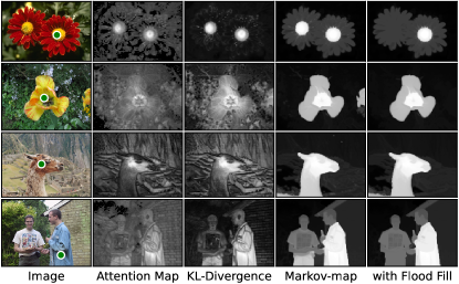
Figure 2: Comparison of semantic maps. Each map is generated from a single prompt point. For better comparison, we use nearest-neighbor interpolation based upscaling of the maps and Markov-maps are inverted such that the lowest value is white and the highest value is black.

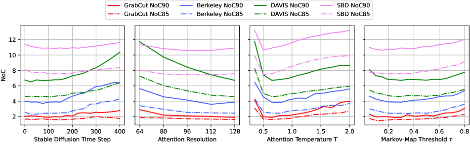
Figure 3: Impact of the hyperparameters of SD and Markov-map, respectively, on all four datasets, each represented by a single color. Dashed lines correspond to NoC85, continues lines to NoC90. The graph of SBD is based on a randomly sampled subset of 500 images.

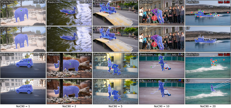
Figure 4: Segmentation examples on DAVIS [27]. Each column shows examples based on the NoC90 value, ranging from easy cases $\mathrm{NoC90}=1$ on the left to difficult cases $\mathrm{NoC90}=10$ and failure cases $\mathrm{NoC90}=20$ on the right. Foreground prompt points are shown in green and background points in red.

4.3 Qualitative Results of M2N2

Fig. 2 compares the semantic maps of our proposed Markov-maps with the other baselines. We observe that Markov-maps are less noisy, have clearer semantic boundaries, and have more uniform values within semantically similar regions. Additionally, we notice that Markov-maps nicely reflect a semantic hierarchy due to the segment size ambiguity of a single prompt point. For example, in the first row and right-most column, the two overlapping flowers have three clearly separated hierarchy levels. Each hierarchical level can be selected by setting a corresponding threshold $\lambda$. The first level contains the right flower’s ovary, the second contains both flowers together and the final level covers everything. The two overlapping flowers also show the strengths and weaknesses of our flood fill approach. It enables instance segmentation of the right flower’s ovary by suppressing the local minimum of the left flower’s ovary. On the other hand, flood fill would fail to segment the individual instances of the flowers, because they are overlapping. Please note that M2N2 can still segment overlapping instances by utilizing multiple prompt points.

Looking at segmentation examples of the DAVIS dataset in Fig. 4, we observe a similar issue in the $\mathrm{NoC90}=10$ case, where a single dancer is in front of a semantically similar crowd. An additional disadvantage of flood fill is that obstructions can result in splitting instances into multiple areas. As an example, the segmentation of the rhinoceros requires two prompt points, instead of one, as the obstructing tree splits the instance into two separate regions. Due to the limited attention resolution, M2N2 faces challenges in segmenting thin and fine structures, as shown in the rightmost column. In general, we observe that M2N2 generates consistent segments with sharp semantic boundaries without being trained on any segmentation labels.

5 Conclusion

We proposed M2N2, a novel method for unsupervised training-free point prompt based interactive segmentation. By interpreting an aggregated self-attention tensor of Stable Diffusion 2 as a Markov transition operator, we generated semantically rich Markov-maps. We showed that Markov-maps have less noise, clearer semantic boundaries, and more uniform values for semantically similar regions. By combining Markov-maps with truncated nearest neighbor, we developed M2N2, which even outperformed state-of-the-art unsupervised training-based methods in most of the datasets. Current limitations are the segmentation of fine structures due to low attention resolution, as well as overlapping or obstructed segments, where M2N2 may require more prompt points. Therefore, future work may involve using higher attention resolutions and improving instance separation.

References

- Bai and Sapiro [2009] Xue Bai and Guillermo Sapiro. Geodesic matting: A framework for fast interactive image and video segmentation and matting. Int. J. Comput. Vision, 82(2):113–132, 2009.
- Caron et al. [2021] Mathilde Caron, Hugo Touvron, Ishan Misra, Herv’e J’egou, Julien Mairal, Piotr Bojanowski, and Armand Joulin. Emerging properties in self-supervised vision transformers. 2021 IEEE/CVF International Conference on Computer Vision (ICCV), pages 9630–9640, 2021.
- Chen et al. [2023] Shoufa Chen, Pei Sun, Yibing Song, and Ping Luo. Diffusiondet: Diffusion model for object detection. In IEEE/CVF International Conference on Computer Vision (ICCV), 2023.
- Chen et al. [2021] Xi Chen, Zhiyan Zhao, Feiwu Yu, Yilei Zhang, and Manni Duan. Conditional diffusion for interactive segmentation. In Proceedings of the IEEE/CVF International Conference on Computer Vision (ICCV), pages 7345–7354, 2021.
- Chen et al. [2022] Xi Chen, Zhiyan Zhao, Yilei Zhang, Manni Duan, Donglian Qi, and Hengshuang Zhao. FocalClick: Towards Practical Interactive Image Segmentation . In 2022 IEEE/CVF Conference on Computer Vision and Pattern Recognition (CVPR), pages 1290–1299, Los Alamitos, CA, USA, 2022. IEEE Computer Society.
- Dosovitskiy et al. [2021] Alexey Dosovitskiy, Lucas Beyer, Alexander Kolesnikov, Dirk Weissenborn, Xiaohua Zhai, Thomas Unterthiner, Mostafa Dehghani, Matthias Minderer, Georg Heigold, Sylvain Gelly, Jakob Uszkoreit, and Neil Houlsby. An image is worth 16x16 words: Transformers for image recognition at scale. In 9th International Conference on Learning Representations, ICLR 2021, Virtual Event, Austria, May 3-7, 2021. OpenReview.net, 2021.
- Grady [2006] Leo Grady. Random walks for image segmentation. IEEE Trans. Pattern Anal. Mach. Intell., 28(11):1768–1783, 2006.
- Gulshan et al. [2010] Varun Gulshan, Carsten Rother, Antonio Criminisi, Andrew Blake, and Andrew Zisserman. Geodesic star convexity for interactive image segmentation. In 2010 IEEE Computer Society Conference on Computer Vision and Pattern Recognition, pages 3129–3136, 2010.
- Hamilton et al. [2022] Mark Hamilton, Zhoutong Zhang, Bharath Hariharan, Noah Snavely, and William T. Freeman. Unsupervised semantic segmentation by distilling feature correspondences. In International Conference on Learning Representations (ICLR), 2022.
- Hao et al. [2021] Yuying Hao, Yi Liu, Zewu Wu, Lin Han, Yizhou Chen, Guowei Chen, Lutao Chu, Shiyu Tang, Zhiliang Yu, Zeyu Chen, and Baohua Lai. Edgeflow: Achieving practical interactive segmentation with edge-guided flow. 2021 IEEE/CVF International Conference on Computer Vision Workshops (ICCVW), pages 1551–1560, 2021.
- Hariharan et al. [2011] Bharath Hariharan, Lubomir Bourdev, Pablo Arbelaez, Jitendra Malik, and Subhransu Maji. Semantic contours from inverse detectors . In 2011 IEEE International Conference on Computer Vision (ICCV 2011), pages 991–998, Los Alamitos, CA, USA, 2011. IEEE Computer Society.
- He et al. [2021] Kaiming He, Xinlei Chen, Saining Xie, Yanghao Li, Piotr Doll’ar, and Ross B. Girshick. Masked autoencoders are scalable vision learners. 2022 IEEE/CVF Conference on Computer Vision and Pattern Recognition (CVPR), pages 15979–15988, 2021.
- Jang and Kim [2019] Won-Dong Jang and Chang-Su Kim. Interactive image segmentation via backpropagating refinement scheme. In 2019 IEEE/CVF Conference on Computer Vision and Pattern Recognition (CVPR), pages 5292–5301, 2019.
- Ke et al. [2023] Bingxin Ke, Anton Obukhov, Shengyu Huang, Nando Metzger, Rodrigo Caye Daudt, and Konrad Schindler. Repurposing diffusion-based image generators for monocular depth estimation. 2024 IEEE/CVF Conference on Computer Vision and Pattern Recognition (CVPR), pages 9492–9502, 2023.
- Kirillov et al. [2023] Alexander Kirillov, Eric Mintun, Nikhila Ravi, Hanzi Mao, Chloe Rolland, Laura Gustafson, Tete Xiao, Spencer Whitehead, Alexander C. Berg, Wan-Yen Lo, Piotr Dollár, and Ross Girshick. Segment anything. In 2023 IEEE/CVF International Conference on Computer Vision (ICCV), pages 3992–4003, 2023.
- Kopf et al. [2007] Johannes Kopf, Michael F. Cohen, Dani Lischinski, and Matthew Uyttendaele. Joint bilateral upsampling. ACM SIGGRAPH 2007 papers, 2007.
- Li et al. [2023a] Alexander C. Li, Mihir Prabhudesai, Shivam Duggal, Ellis Brown, and Deepak Pathak. Your Diffusion Model is Secretly a Zero-Shot Classifier . In 2023 IEEE/CVF International Conference on Computer Vision (ICCV), pages 2206–2217, Los Alamitos, CA, USA, 2023a. IEEE Computer Society.
- Li et al. [2023b] Kehan Li, Yian Zhao, Zhennan Wang, Zesen Cheng, Peng Jin, Xiang Ji, Li ming Yuan, Chang Liu, and Jie Chen. Multi-granularity interaction simulation for unsupervised interactive segmentation. 2023 IEEE/CVF International Conference on Computer Vision (ICCV), pages 666–676, 2023b.
- Li et al. [2024] Xiang Li, Chung-Ching Lin, Yinpeng Chen, Zicheng Liu, Jinglu Wang, Rita Singh, and Bhiksha Raj. Paintseg: training-free segmentation via painting. In Proceedings of the 37th International Conference on Neural Information Processing Systems, Red Hook, NY, USA, 2024. Curran Associates Inc.
- Lin et al. [2020] Zheng Lin, Zhao Zhang, Lin-Zhuo Chen, Ming-Ming Cheng, and Shao-Ping Lu. Interactive image segmentation with first click attention. In 2020 IEEE/CVF Conference on Computer Vision and Pattern Recognition (CVPR), pages 13336–13345, 2020.
- Lin et al. [2022] Zheng Lin, Zheng-Peng Duan, Zhao Zhang, Chun-Le Guo, and Ming-Ming Cheng. Focuscut: Diving into a focus view in interactive segmentation. In Proceedings of the IEEE/CVF Conference on Computer Vision and Pattern Recognition (CVPR), pages 2637–2646, 2022.
- Liu et al. [2024] Jie Liu, Haochen Wang, Wenzhe Yin, Jan-Jakob Sonke, and Efstratios Gavves. Click prompt learning with optimal transport for interactive segmentation. In European Conference on Computer Vision (ECCV), 2024.
- Liu et al. [2023] Qin Liu, Zhenlin Xu, Gedas Bertasius, and Marc Niethammer. Simpleclick: Interactive image segmentation with simple vision transformers. In Proceedings. IEEE International Conference on Computer Vision, pages 22233–22243, 2023.
- Long et al. [2015] Jonathan Long, Evan Shelhamer, and Trevor Darrell. Fully convolutional networks for semantic segmentation. In 2015 IEEE Conference on Computer Vision and Pattern Recognition (CVPR), pages 3431–3440, 2015.
- Martin et al. [2001] D. Martin, C. Fowlkes, D. Tal, and J. Malik. A database of human segmented natural images and its application to evaluating segmentation algorithms and measuring ecological statistics. In Computer Vision, 2001. ICCV 2001. Proceedings. Eighth IEEE International Conference on, pages 416–423 vol.2, 2001.
- Melas-Kyriazi et al. [2022] Luke Melas-Kyriazi, Christian Rupprecht, Iro Laina, and Andrea Vedaldi. Deep spectral methods: A surprisingly strong baseline for unsupervised semantic segmentation and localization. In 2022 IEEE Conference on Computer Vision and Pattern Recognition (CVPR), 2022.
- Perazzi et al. [2016] Federico Perazzi, Jordi Pont-Tuset, Brian McWilliams, Luc Van Gool, Markus Gross, and Alexander Sorkine-Hornung. A benchmark dataset and evaluation methodology for video object segmentation. In Proceedings of the IEEE Conference on Computer Vision and Pattern Recognition (CVPR), 2016.
- Ravi et al. [2024] Nikhila Ravi, Valentin Gabeur, Yuan-Ting Hu, Ronghang Hu, Chaitanya Ryali, Tengyu Ma, Haitham Khedr, Roman Rädle, Chloe Rolland, Laura Gustafson, Eric Mintun, Junting Pan, Kalyan Vasudev Alwala, Nicolas Carion, Chao-Yuan Wu, Ross Girshick, Piotr Dollár, and Christoph Feichtenhofer. Sam 2: Segment anything in images and videos, 2024.
- Rombach et al. [2022] Robin Rombach, Andreas Blattmann, Dominik Lorenz, Patrick Esser, and Björn Ommer. High-resolution image synthesis with latent diffusion models. In Proceedings of the IEEE/CVF Conference on Computer Vision and Pattern Recognition, pages 10684–10695, 2022.
- Ross [1997] Sheldon M. Ross. Introduction to Probability Models. Academic Press, San Diego, CA, USA, sixth edition, 1997.
- Rother et al. [2004] Carsten Rother, Vladimir Kolmogorov, and Andrew Blake. ”grabcut”: interactive foreground extraction using iterated graph cuts. In ACM SIGGRAPH 2004 Papers, page 309–314, New York, NY, USA, 2004. Association for Computing Machinery.
- Shi and Malik [2000] Jianbo Shi and J. Malik. Normalized cuts and image segmentation. IEEE Trans. on Pattern Analysis and Machine Intelligence, 22(8):888–905, 2000.
- Siméoni et al. [2021] Oriane Siméoni, Gilles Puy, Huy V. Vo, Simon Roburin, Spyros Gidaris, Andrei Bursuc, Patrick P’erez, Renaud Marlet, and Jean Ponce. Localizing objects with self-supervised transformers and no labels. ArXiv, abs/2109.14279, 2021.
- Sinkhorn [1964] Richard Sinkhorn. A Relationship Between Arbitrary Positive Matrices and Doubly Stochastic Matrices. The Annals of Mathematical Statistics, 35(2):876 – 879, 1964.
- Sofiiuk et al. [2020] Konstantin Sofiiuk, Ilya A. Petrov, Olga Barinova, and Anton Konushin. F-brs: Rethinking backpropagating refinement for interactive segmentation. In IEEE Conference on Computer Vision and Pattern Recognition (CVPR). IEEE, 2020.
- Sofiiuk et al. [2022] Konstantin Sofiiuk, Ilia Petrov, and Anton Konushin. Reviving iterative training with mask guidance for interactive segmentation. In 2022 IEEE International Conference on Image Processing (ICIP), 2022.
- Sun et al. [2024] Shoukun Sun, Min Xian, Fei Xu, Luca Capriotti, and Tiankai Yao. Cfr-icl: Cascade-forward refinement with iterative click loss for interactive image segmentation. In Technical Tracks 14, number 5 in Proceedings of the AAAI Conference on Artificial Intelligence, pages 5017–5024. Association for the Advancement of Artificial Intelligence, 2024. Publisher Copyright: Copyright © 2024, Association for the Advancement of Artificial Intelligence.; 38th AAAI Conference on Artificial Intelligence, AAAI 2024 ; Conference date: 20-02-2024 Through 27-02-2024.
- Tian et al. [2023] Junjiao Tian, Lavisha Aggarwal, Andrea Colaco, Zsolt Kira, and Mar González-Franco. Diffuse, attend, and segment: Unsupervised zero-shot segmentation using stable diffusion. 2024 IEEE/CVF Conference on Computer Vision and Pattern Recognition (CVPR), pages 3554–3563, 2023.
- Wang et al. [2021] Xinlong Wang, Rufeng Zhang, Chunhua Shen, Tao Kong, and Lei Li. Dense contrastive learning for self-supervised visual pre-training. In Proc. IEEE Conf. Computer Vision and Pattern Recognition (CVPR), 2021.
- Wang et al. [2022a] Xinlong Wang, Zhiding Yu, Shalini De Mello, Jan Kautz, Anima Anandkumar, Chunhua Shen, and Jose M. Alvarez. Freesolo: Learning to segment objects without annotations. In Proceedings of the IEEE/CVF Conference on Computer Vision and Pattern Recognition (CVPR), pages 14176–14186, 2022a.
- Wang et al. [2024] Xudong Wang, Jingfeng Yang, and Trevor Darrell. Segment anything without supervision. In The Thirty-eighth Annual Conference on Neural Information Processing Systems, 2024.
- Wang et al. [2022b] Yangtao Wang, XI Shen, Shell Xu Hu, Yuan Yuan, James L. Crowley, and Dominique Vaufreydaz. Self-supervised transformers for unsupervised object discovery using normalized cut. 2022 IEEE/CVF Conference on Computer Vision and Pattern Recognition (CVPR), pages 14523–14533, 2022b.
- Wang et al. [2022c] Yangtao Wang, Xiaoke Shen, Yuan Yuan, Yuming Du, Maomao Li, Shell Xu Hu, James L. Crowley, and Dominique Vaufreydaz. Tokencut: Segmenting objects in images and videos with self-supervised transformer and normalized cut. IEEE Transactions on Pattern Analysis and Machine Intelligence, 45:15790–15801, 2022c.
- Xu et al. [2016] Ning Xu, Brian Price, Scott Cohen, Jimei Yang, and Thomas Huang. Deep interactive object selection. In 2016 IEEE Conference on Computer Vision and Pattern Recognition (CVPR), pages 373–381, 2016.
- Yang et al. [2024] Lihe Yang, Xiaogang Xu, Bingyi Kang, Yinghuan Shi, and Hengshuang Zhao. Freemask: synthetic images with dense annotations make stronger segmentation models. In Proceedings of the 37th International Conference on Neural Information Processing Systems, Red Hook, NY, USA, 2024. Curran Associates Inc.
- Zhou et al. [2023] Minghao Zhou, Hong Wang, Qian Zhao, Yuexiang Li, Yawen Huang, Deyu Meng, and Yefeng Zheng. Interactive segmentation as gaussian process classification. 2023 IEEE/CVF Conference on Computer Vision and Pattern Recognition (CVPR), pages 19488–19497, 2023.