Breakdown of homoclinic orbits to $L_{1}$ of the hydrogen atom in a circularly polarized microwave field

Abstract

We consider the Rydberg electron in a circularly polarized microwave field, whose dynamics is described by a 2 d.o.f. Hamiltonian, which is a perturbation of size $K>0$ of the standard rotating Kepler problem. In a rotating frame, the largest chaotic region of this system lies around a center-saddle equilibrium point $L_{1}$ and its associated invariant manifolds. We compute the distance between stable and unstable manifolds of $L_{1}$ by means of a semi-analytical method, which consists of combining normal form, Melnikov, and averaging methods with numerical methods. Also, we introduce a new family of Hamiltonians, which we call Toy CP systems, to be able to compare our numerical results with the existing theoretical results in the literature. It should be noted that the distance between these stable and unstable manifolds is exponentially small in the perturbation parameter $K$ (in analogy with the $L_{3}$ libration point of the R3BP).

1 Introduction

1.1 State of the art of the CP Problem

The CP Problem consists of the motion in an hydrogen atom placed in an external circularly polarized microwave field. This system has been intensively studied, both experimentally [18, 36, 8], as theoretically, from classical [34, 33, 19, 28, 32] and quantum [19, 37, 9] points of view, as well as numerically [23, 11, 20, 16, 10, 6, 31, 7]. In a rotating frame (see Section 1.2), the CP problem reads as a 2 degree-of-freedom (d.o.f.) Hamiltonian system. For a small enough field strength or a large enough angular frequency of the microwave field, the CP problem turns out to be just a perturbation of some size, say $K>0$, of the rotating Kepler problem, and by KAM theory the phase space is pretty full of 2-dimensional invariant tori with non-conmensurable frequencies. These 2-dimensional KAM tori preclude the existence of unstable trajectories, and in particular of ionization, that is, the loss of the electron, which turns out to be the main topic dealt with in all these studies. Consequently, ionization only takes place when all KAM invariant tori break, which happens when the perturbation parameter $K$ is not so small.

However, for small $K$, the motion is not completely regular, and erratic trajectories can appear. Such kind of chaotic motion takes place outside the KAM tori, and is typically associated with the existence of saddle invariant objects. There are, at least, three zones where saddle objects may appear in the CP problem: (i) near collision with the nucleus, inside the first KAM torus, (ii) very far of the nucleus, say at infinity, outside the last KAM torus, and (iii) in the resonant zones, between the KAM invariant tori.

The aim of this work is to study the largest chaotic resonance zone, which happens to be associated with the lowest-order commensurability of the frequencies of the unperturbed invariant tori, and takes place around a saddle-center equilibrium point in a rotating frame, called $L_{1}$, together with its associated invariant unstable and stable manifolds. Saddle Lyapunov periodic orbits emerge from $L_{1}$, which are very important, indeed crucial, for the global behavior of the system [6]. Indeed, it is a standard principle in dynamical systems that the saddle invariant objects and their associated invariant manifolds are the main landmarks for understanding the global dynamical behavior of a dynamical system.

Using an adequate cross-section, we measure the distance between the two branches of unstable and stable asymptotic trajectories to $L_{1}$, which turns out to be positive and exponentially small with respect to the perturbation parameter $K$. This is a consequence of the fact that $L_{1}$ is a weak saddle equilibrium point, that is, its real characteristic exponents are $\pm\Ord{\sqrt{K}}$, so they tend to zero when the size of the perturbation $K$ tends to zero. The measure of this distance is performed both analytically (31) and numerically (6–7) with a fairly good agreement, although its exponentially smallness makes difficult a very precise fitting.

The numerical measure requires using high-precision computations combined with the parameterization method (described in Appendix B) to get a local computation of the invariant manifolds, as well as Taylor method (implemented on a robust, fast and accurate package by Jorba and Zou [29]) to integrate the system without a significant loss of precision. Multiple precision computations have been carried out using the mpfr library (see [17]).

Analytic approximations are also obtained for the invariant manifolds of $L_{1}$. For this, we simply introduce action-angle variables, which are nothing more than the Delaunay variables for the Kepler problem, combined with a subsequent change to the Poincaré variables to avoid the degeneracy of the circular solutions of Kepler’s problem. In these variables, the CP problem consists of a perturbation of an integrable system formed by an isochronous rotor plus an amended pendulum. This amended pendulum depends on the perturbation parameter and gives rise to two separatrices, which also depend on the perturbation parameter.

When the perturbation is taken into account, we introduce a direct approximation of the splitting of these separatrices, based on the study of the variational equations along them (this is the so-called Melnikov method) and we compare the distance between these approximate invariant manifolds with the one obtained with the aforementioned numerical calculations, performed both in synodic coordinates (6) for the rotating frame (in the Poincaré section $y=0$), and in Poincaré variables (7).

We have also verified that to have a good analytical approximation, it is crucial to choose the right amended pendulum. For this reason we also present an additional approximation equivalent to Melnikov method, based on the application of the averaging method. We check that the choice of an adequate degree of the amended pendulum as a function of the perturbation parameter is totally necessary to obtain a good fit with the numerical calculations.

Unfortunately, there are no theoretical results in the literature that can be directly applied to prove analytically the numerical results found for the CP problem, due to the fact that the perturbation presents a high-order singularity, and that the integrable Hamiltonian where perturbative theoretical methods should be applied depends essentially on the perturbative parameter $K$. To discuss whether Melnikov method, when applied to a Hamiltonian given by an integrable part plus a perturbation, correctly predicts the found fitting formulas, it is necessary to consider both the integrable part and the perturbation.

This discussion has led us to the analysis of a more general Hamiltonian that we have called Toy CP problem (9), which, apart from $K$, also depends on two other parameters $a$ and $m$. More details are provided in subsection 1.4. The observed phenomenology opens the door to a new world of theoretical studies.

It has to be noticed that the distance studied is much smaller in one of the separatrix, the internal one, than in the other one, the external separatrix. For this reason, in this paper we focus on measuring the distance between the external asymptotic trajectories to $L_{1}$.

This is a first step to measuring the distance between the two branches of asymptotic unstable and stable surfaces to the Lyapunov periodic orbits close to $L_{1}$, and to show that they intersect along only two transverse homoclinic orbits. This computation will be performed in a future paper, and will provide a measure of the chaotic region close to $L_{1}$, which is proportional to the transversality of these branches.

It is worth remarking that the CP problem is similar to the Planar Circular Restricted 3-Body Problem (R3BP), since both are perturbations of the rotational Kepler problem. Since the equilibrium point $L_{1}$ of the CP problem is weakly hyperbolic, it is also similar to the libration point $L_{3}$ of the R3BP, where similar features happen and theoretical results are available [2, 3]. Therefore, we have applied a number of tools coming from Celestial Mechanics or, more generically, Hamiltonian systems, like invariant manifolds, Melnikov method, averaging method, etc.

1.2 The model for the CP problem

In the simplest case (assuming planar motion for the electron) the classical motion is governed by a system of two 2nd-order ODE

$$\begin{split}\ddot{X}&=-\dfrac{X}{R^{3}}-F\cos\left(\oomega s\right),\qquad R^{2}=X^{2}+Y^{2},\\ \ddot{Y}&=-\dfrac{Y}{R^{3}}-F\sin\left(\oomega s\right),\qquad\dot{}=\frac{\df{}}{\df{s}},\end{split}$$

where $\oomega>0$ is the angular frequency of the microwave field and $F>0$ is the field strength.

This system can be written as a periodic in time 2 d.o.f Hamiltonian

$$H(X,Y,P_{X},P_{Y})=\frac{1}{2}\left(P_{X}^{2}+P_{Y}^{2}\right)-\frac{1}{R}+F\left(X\cos\left(\oomega s\right)+Y\sin\left(\oomega s\right)\right).$$

As in the R3BP (Restricted 3-Body Problem), we can get rid of the time dependence introducing rotating coordinates $\left(\widetilde{X},\widetilde{Y},P_{\widetilde{X}},P_{\widetilde{Y}},s\right)$

$$\begin{pmatrix}\widetilde{X}\\ \widetilde{Y}\end{pmatrix}=R(\oomega s)\begin{pmatrix}X\\ Y\end{pmatrix},\quad\begin{pmatrix}P_{\widetilde{X}}\\ P_{\widetilde{Y}}\end{pmatrix}=R(\oomega s)\begin{pmatrix}P_{X}\\ P_{Y}\end{pmatrix},\quad R(\oomega s)=\begin{pmatrix}\cos\oomega s&\sin\oomega s\\ -\sin\oomega s&\cos\oomega s\end{pmatrix}$$

to get an autonomous Hamiltonian

$$H\left(\widetilde{X},\widetilde{Y},P_{\widetilde{X}},P_{\widetilde{Y}}\right)=\frac{1}{2}\left(P_{\widetilde{X}}^{2}+P_{\widetilde{Y}}^{2}\right)-\frac{1}{\widetilde{R}}-\oomega\left(\widetilde{X}P_{\widetilde{Y}}-\widetilde{Y}P_{\widetilde{X}}\right)+F\widetilde{X},$$

where $\widetilde{R}^{2}=\widetilde{X}^{2}+\widetilde{Y}^{2}$. To get rid of the angular frequency $\oomega$ we perform the change $(\widetilde{X},\widetilde{Y})=a(\mathpzc x,\mathpzc y)$, $\left(P_{\widetilde{X}},P_{\widetilde{Y}}\right)=a\oomega(\mathpzc p_{\mathpzc x},\mathpzc p_{\mathpzc y})$, which is a symplectic transformation with multiplier $a^{2}\oomega$ with $a=1/\oomega^{2/3}$, plus a scaling in time $t=\oomega s$ to get a new Hamiltonian in the rotating and scaled coordinates $(\mathpzc x,\mathpzc y,\mathpzc p_{\mathpzc x},\mathpzc p_{\mathpzc y})$, usually also called synodic coordinates in the literature.

$$H(\mathpzc x,\mathpzc y,\mathpzc p_{\mathpzc x},\mathpzc p_{\mathpzc y})=\frac{1}{2}(\mathpzc p_{\mathpzc x}^{2}+\mathpzc p_{\mathpzc y}^{2})-\frac{1}{r}-(\mathpzc x\mathpzc p_{\mathpzc y}-\mathpzc y\mathpzc p_{\mathpzc x})+K\mathpzc x,\qquad r=\sqrt{\mathpzc x^{2}+\mathpzc y^{2}},$$ (1)

where $K=F/\oomega^{4/3}>0$, with associated Hamiltonian equations

$$\dot{\mathpzc}x =\mathpzc p_{\mathpzc x}+\mathpzc y, \dot{\mathpzc p_{\mathpzc x}} =\mathpzc p_{\mathpzc y}-\frac{\mathpzc x}{r^{3}}-K,$$ (2)

$$\dot{\mathpzc}y =\mathpzc p_{\mathpzc y}-\mathpzc x, \dot{\mathpzc p_{\mathpzc y}} =-\mathpzc p_{\mathpzc x}-\frac{\mathpzc y}{r^{3}}.$$

It is very important and useful to realize that this Hamiltonian system is invariant under the reversibility

$$(t,\mathpzc x,\mathpzc y,\mathpzc p_{\mathpzc x},\mathpzc p_{\mathpzc y})\mapsto(-t,\mathpzc x,-\mathpzc y,-\mathpzc p_{\mathpzc x},\mathpzc p_{\mathpzc y}).$$ (3)

Note that for $K=0$ we get just the rotating Kepler Hamiltonian. Although the parameter $K$ only appears, additively, in the equation of the momentum $\mathpzc p_{\mathpzc x}$ of equations (2), for $K>0$ the CP system is much more complicated than the rotating Kepler problem, as we will describe below.

In the literature, it is also typical to find the system associated with the Hamiltonian (1) written as a system of second-order ODE

$$\left\{\begin{aligned} &\ddot{\mathpzc x}-2\dot{\mathpzc y}=\Omega x(\mathpzc x,\mathpzc y),\\ &\ddot{\mathpzc y}+2\dot{\mathpzc x}=\Omega y(\mathpzc x,\mathpzc y),\end{aligned}\right.$$ (4)

where

$$\Omega(\mathpzc x,\mathpzc y)=\frac{1}{2}r^{2}+\frac{1}{r}-K\mathpzc x,$$

and $r=\sqrt{\mathpzc x^{2}+\mathpzc y^{2}}$. In this way, the system (4) has a first integral, known as the Jacobi first integral, defined by

$$C=2\Omega(\mathpzc x,\mathpzc y)-(\dot{\mathpzc x}^{2}+\dot{\mathpzc y}^{2}),$$ (5)

and related to the Hamiltonian (1) by $C=-2H$. For a fixed value of $K$ and the first integral $C$, the admissible regions of motion, known as Hill regions, are defined by

$$\mathcal{R}=\mathcal{R}(K,C)=\left\{(\mathpzc x,\mathpzc y)\in\R^{2}\,|\,2\Omega(\mathpzc x,\mathpzc y)\geq C\right\}.$$

1.3 Invariant objects

The equations for equilibrium points $\dot{\mathpzc}x=\dot{\mathpzc}y=\dot{\mathpzc}p_{\mathpzc x}=\dot{\mathpzc}p_{\mathpzc y}=0$ in system (2) are just

$$\mathpzc p_{\mathpzc x}=-\mathpzc y,\ \mathpzc p_{\mathpzc y}=\mathpzc x,\ \ \mathpzc x-\frac{\mathpzc x}{r^{3}}=K,\ \mathpzc y-\frac{\mathpzc y}{r^{3}}=0,$$

which give a whole circle $r=1$ for $K=0$, that is, for the rotating Kepler Hamiltonian. For the CP problem $K>0$ there are just two equilibrium points

$$L_{1}=(\mathpzc x_{1},0,0,\mathpzc x_{1}),\qquad L_{2}=(\mathpzc x_{2},0,0,\mathpzc x_{2}),$$

with $\mathpzc x_{1}^{3}-K\mathpzc x_{1}^{2}-1=0$ and $\mathpzc x_{2}^{3}-K\mathpzc x_{2}^{2}+1=0$ so that $\mathpzc x_{1}=\mathpzc x_{1}(K)$, $\mathpzc x_{2}=\mathpzc x_{2}(K)$ are of the form

$$\mathpzc x_{1}(K)=-1+\frac{K}{3}+\Ord{K^{2}},\qquad\mathpzc x_{2}(K)=\mathpzc x_{1}(-K)=-1+\frac{K}{3}+\Ord{K^{2}}.$$

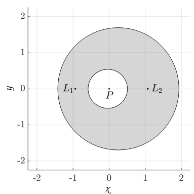
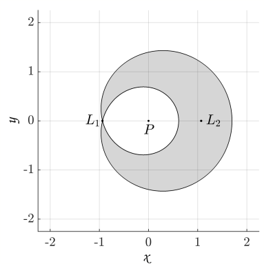
Figure 1: In gray the forbidden region of motion for $K=0.2$ and $H=-2<h_{1}$, $H=h_{1}$ and $H=-1.5\in(h_{1},h_{2})$ from left to right. $P$ denotes the position of the nucleus.

Since $L_{i}$ are critical points of the potential, the topology of the Hill regions changes at the values of the Jacobi constant corresponding to these points, or equivalently, at the values $h_{i}=H(L_{i})$ of the Hamiltonian (1), for $i=1,2$.

Note that for values $H\leq h_{1}$, ionization cannot occur, and for values $H\geq h_{2}$, the entire configuration space becomes a valid region of motion (see Figure 1). This is of significant importance, as the point $L_{1}$ and the dynamics associated with the invariant objects emanating from it act as the channel for ionization at the lowest energy levels where it is possible.

In particular, $L_{1}$ is a center-saddle equilibrium point for all $K>0$, with characteristic exponents

$$\pm\iu(1+K)(1+\Ord{K}),\quad\pm\sqrt{3K}(1+\Ord{K}),$$

and associated 1D invariant manifolds, $\Cu(L_{1}),\Cs(L_{1})$ for $h_{1}$. Emerging form $L_{1}$ there is a family of saddle Lyapunov periodic orbits $OL$ around $L_{1}$ for $h>h_{1}$, with associated 2D-invariant manifolds $W^{\un}(OL),W^{\st}(OL)$, also called whiskers.

Notice that the saddle character of $L_{1}$ is weak with respect to the parameter $K$, because its saddle characteristic exponents $\pm\sqrt{3K}(1+\Ord{K})$ tend to $0$ as $K$ tends to $0$. This will imply a very small distance between $\Cu(L_{1})$ and $\Cs(L_{1})$ and a very small transversality between $W^{\un}(OL)$ and $W^{\st}(OL)$, indeed exponentially small in $K$. This weak saddle character of $L_{1}$ is totally analogous to the weak saddle character of the libration point $L_{3}$ of the R3BP.

In this paper, we will focus only on the invariant manifolds $\Cu(L_{1}),\Cs(L_{1})$. We distinguish between the external branches of the manifolds, $W^{\un,\mathrm{e}}(L_{1})$, $W^{\st,\mathrm{e}}(L_{1})$ and the internal branches $W^{\un,\mathrm{i}}(L_{1})$, $W^{\st,\mathrm{i}}(L_{1})$. The four different branches for $K=0.1$, $0.01$ and $0.001$ are displayed in Figure 2. Notice that the external branches seem to coincide (similarly the internal ones) but they do not. Precisely, the purpose of this paper is to analyze the small distance—splitting—between them.

Actually we will concentrate on the external branches that will be simply denoted, from now on, by $\Cu(L_{1}),\Cs(L_{1})$ (unless there are possible misunderstandings).

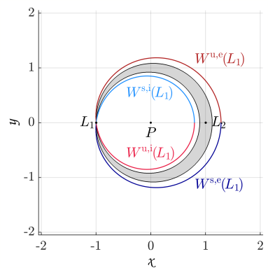
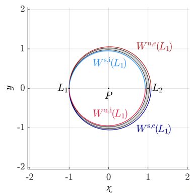
Figure 2: $(\mathpzc x,\mathpzc y)$ projection of the external $W^{\un,\mathrm{e}}(L_{1})$ and internal $W^{\un,\mathrm{i}}(L_{1})$ unstable manifolds of $L_{1}$ (similarly for the stable ones) for $K=0.1$, $0.01$ and $0.001$ from left to right. In gray the forbidden region of motion for $h_{1}$.

1.4 Main Results

1. We have numerically found an asymptotic formula for the splitting between the invariant unstable and stable manifolds (external branches) of $L_{1}$, $W^{\un,\st}(L_{1})$, at (the first crossing with) $\mathpzc y=0$ in synodic (rotating) coordinates $(\mathpzc x,\mathpzc y,\dot{\mathpzc x},\dot{\mathpzc y})$ (2), which has the expression

   $$\Delta\dot{\mathpzc}x\sim\varepsilon A\omega^{r}\exp\left(\frac{\omega\pi}{2}\right),\qquad\varepsilon=\left(\frac{K}{3}\right)^{1/4},\quad\omega=-\frac{1}{3\varepsilon^{2}}=-\frac{1}{\sqrt{3K}},$$ (6)

   with $r=1.61111\ldots=29/18$ and the leading constant $A=16.055307843\dots$ See (39) and (42) in subsection 3.2.

2. We obtain a similar asymptotic formula for the same splitting but computed in Poincaré (or resonant) variables $(x,y,q,p)$, (11) and (14),

   $$\Delta p\sim\varepsilon\bar{A}\omega^{\bar{r}}\exp\left(\frac{\omega\pi}{2}\right),$$ (7)

   see (43), with $\bar{r}=2.11111\ldots=19/9=r+1/2$ and the leading constant $\bar{A}=27.80860891\dots$ (see (46) in subsection 3.3), where the addition of $1/2$ to $r$ to get $\bar{r}$ is due to the non-canonical change (11) from synodic to resonant variables. See (48) in subsection 3.3.

3. We emphasize the “key point” of the resonant variables: the analysis of the behavior of the invariant manifolds $W^{\un,\st}(L_{1})$ for the CP problem can be regarded as the behavior of a perturbation of a homoclinic separatrix. Indeed, the Hamiltonian in the resonant variables is

   $$H(x,y,q,p)=\omega\frac{q^{2}+p^{2}}{2}+\frac{y^{2}}{2}+\cos x-1+\varepsilon H_{1}(x,y,q,p;\varepsilon),$$

   and the homoclinic separatrix is given by $q=p=0$ and (20).

4. We show numerically that the Melnikov method predicts correctly the numerical asymptotic results (7), as long as we take a suitable integrable Hamiltonian system, formed by a rotor and an amended pendulum, which is not the natural pendulum (as happens in a lot of other problems, see, for instance, [35, 25, 4, 24]). To do so, we consider a truncated Hamiltonian once we have applied a change of variables (from synodic to Poincaré ones). More precisely,

   $$H(x,y,q,p)=\omega\frac{q^{2}+p^{2}}{2}+\frac{y^{2}}{2}+\cos x-1-\frac{2}{3}\varepsilon^{2}y^{3}+\varepsilon\left(\frac{3q}{2}-\frac{q}{2}\cos 2x-\frac{p}{2}\sin 2x\right),$$ (8)

5. We introduce a new family of perturbations of a rotor and a pendulum, which we call Toy CP problem

   $$H(x,y,q,p)=\omega\frac{q^{2}+p^{2}}{2}+\frac{y^{2}}{2}+\cos x-1-\frac{2a}{3}\varepsilon^{2}y^{3}+\varepsilon^{m}\left(\frac{3q}{2}-\frac{q}{2}\cos 2x-\frac{p}{2}\sin 2x\right),$$ (9)

   in order to check if our results could be provided by previous analytical results in the literature. For $m=1$ Hamiltonian (9) is just the truncated Hamiltonian  (8) of the CP problem after a normal form expansion or, equivalently, after an averaging process. It has to be noticed that in the standard application of normal form or averaging, one typically takes $a=0$ because the term $\displaystyle\frac{2a}{3}\varepsilon^{2}y^{3}$ is of higher order than the $O(\varepsilon)$ perturbation.

   Nevertheless, we found out that the numerically computed values of the splitting depend essentially on the parameter $a$. Particularly the exponent $r$ in formula (6). For the purposes of this paper there are, at least, two different scenarios: the “standard” case $a=0$ and the new case $a=1$. Concerning the integrable part of the Hamiltonian (9), for $a=0$ we have a standard pendulum, whereas for $a=1$ we have a new pendulum, that we call amended pendulum. See the motivation for including this value of $a$ in Subsections 4.1.1 and 4.2.

6. For $a=0$ there are theoretical results [1, 5] for Hamiltonian systems with $1+\frac{1}{2}$ degrees of freedom that can be directly applied to the Toy CP problem (9). According to these theoretical results, for $m\geq 4$ the Melnikov prediction with the standard pendulum gives the correct measure (53) for the splitting:

   $$\Delta p\sim-\varepsilon^{m}\frac{8\pi}{3}\omega^{3}\left(1-\frac{2}{\omega^{2}}\right)\frac{\ee^{\pi\omega/2}}{1-\ee^{2\pi\omega}}.$$ (10)

   We have confirmed numerically these theoretical results in Subsection 4.1.1, but we have further found out that the Melnikov prediction gives also the right result for $m>1$ (see  Subsection 4.1, which opens the door to improve the quoted theoretical results).

   Notice that the exponent $r$ of $\omega$ is $3$ in formula (10). Therefore the above Melnikov prediction with $a=0$ clearly does not give the correct result (7) for the CP problem (12), which takes place just for $m=1$.

7. However, for $a=1$, when we have an amended pendulum in Hamiltonian (9), the Melnikov prediction with the amended pendulum coincides with the value (7) of the splitting computed numerically and gives also the right result for $m>1$, both for the exponent $\bar{r}$ (of $\omega$) and the leading constant $\bar{A}$. It is worth noticing that in all formulas the exponential smallness $\ee^{\pi\omega/2}$ is the same. This is due to the fact the distance of the closest complex singularity of the separatrices to the real line is the same up to terms of order $1/\omega^{4}$, see Appendix C. All these computations are detailed in Section 5 and, in particular, illustrated in Figures 11 and 12. This is, perhaps, the main novelty of this paper: the normal form or averaging procedure to transform a Hamiltonian system close to a resonance to a nearly integrable Hamiltonian must be carried out at a higher order than initially expected, and choosing uniquely some selected term. In passing, it is worth mentioning that the Melnikov integral is computed numerically, since we do not have an explicit expression for the separatrix of the amended pendulum.

8. From the numerical simulations done, we can conclude that the Toy CP problem with $a=m=1$ is a simplified model that already describes the splitting $\Delta p$ of the original CP problem in resonant coordinates, as far as asymptotic formulas for $\Delta p$, when $K$ tends to zero, are analyzed. See Subsection 5.3 and, in particular, Figure 14. Finally, we can also conclude that the fitting asymptotic formula obtained for the Melnikov integral provides the same limit value of the exponent $\bar{r}=\mathring{r}=2.111\ldots=19/9$.

2 Some analytical computations

2.1 Polar coordinates

The Hamiltonian of the CP problem

$$H=\frac{1}{2}(\mathpzc p_{\mathpzc x}^{2}+\mathpzc p_{\mathpzc y}^{2})-\frac{1}{r}-(\mathpzc x\mathpzc p_{\mathpzc y}-\mathpzc y\mathpzc p_{\mathpzc x})+K\mathpzc x,\qquad r=\sqrt{\mathpzc x^{2}+\mathpzc y^{2}},$$

takes the form in canonical polar coordinates $(r,\theta,p_{r},p_{\theta})$

$$H=\frac{1}{2}\left(p_{r}^{2}+\frac{p_{\theta}^{2}}{2}\right)-\frac{1}{r}-p_{\theta}+Kr\cos\theta:=H_{\mathrm{K}}-p_{\theta}+Kr\cos\theta.$$

2.2 Delaunay coordinates

In the canonical Delaunay variables $(\ell,g,L,G)$, which are the action-angle variables for the Kepler Hamiltonian $H_{\mathrm{K}}$ we have

$$H=-\frac{1}{2L^{2}}-G+K\left(a\cos(\ell+g)-\frac{3}{2}ae\cos g+\frac{ae}{2}\cos(2\ell+g)+O(e^{2})\right),$$

where $a=L^{2}$ is the semi-major axis and $\displaystyle e=\sqrt{1-\frac{G^{2}}{L^{2}}}$ the eccentricity.

2.3 Resonant coordinates

The equilibrium point $L_{1}$ satisfies $L=G=1$ (for $K=0$). Changing to resonant variables $(x,y,\varphi,I)$, and scaling

$$\ell=x+\pi+\varphi,\quad g=-\varphi,\quad L=1+\eps^{2}y,\quad G=1+\eps^{2}y-\eps^{2}I,$$ (11)

with $\displaystyle\eps=\left(\frac{K}{3}\right)^{1/4}$, as well as averaging (as in [35, 21, 25, 24]), we get the singular resonant Hamiltonian

$$H(x,y,\varphi,I;\eps)=\omega I+P_{\eps}(x,y)+\eps H_{1}(x,y,\varphi,I;\eps),$$ (12)

where $\displaystyle\omega=-\frac{1}{3\eps^{2}}$ and

$$P_{\eps}(x,y) =F(y,\eps)+\cos x-1,$$

$$H_{1}(\varphi,x,I,y;\eps) =\frac{3}{2}\sqrt{2I}\cos\varphi-\frac{1}{2}\sqrt{2I}\cos(2x+\varphi)+O(\eps),$$

with

$$F(y,\eps)=\frac{y^{2}}{2}+\frac{f(\eps^{2}y)}{3\eps^{4}}=\frac{y^{2}}{2}g(\eps^{2}y),$$ (13)

and

$$f(t) =\frac{1}{2(1+t)^{2}}-\frac{1}{2}+t-\frac{3}{2}t^{2}=-2t^{3}+\frac{5}{2}t^{4}+\cdots+(-1)^{n}\frac{n+1}{2}t^{n}+\cdots=O(t^{3}),$$

$$g(t) =1+\frac{2f(t)}{3t^{2}}=1-\frac{4}{3}t+\frac{5}{3}t^{2}+\cdots+(-1)^{m}\frac{m+3}{3}t^{m}+\cdots.$$

Taylor expanding in $\eps$ we have $F(y,\eps)=F_{k}(y,\eps)+O\left(\eps^{2k+2}y^{k+3}\right)$, where

$$F_{0}(y)=\frac{y^{2}}{2},\quad F_{1}(y)=\frac{y^{2}}{2}-\frac{2}{3}\eps^{2}y^{3},\quad F_{2}(y)=\frac{y^{2}}{2}-\frac{2}{3}\eps^{2}y^{3}+\frac{5}{6}\eps^{4}y^{4},$$

and in general

$$F_{k}(y)=\sum_{n=2}^{k+2}(-1)^{n}\frac{n+1}{6}\eps^{2n-4}y^{n}=y^{2}\sum_{m=0}^{k}(-1)^{m}\frac{m+3}{6}\left(\eps^{2}y\right)^{m},\quad k\geq 0.$$

A remarkable property of this Hamiltonian, for our purposes, is that will allow to distinguish an integrable part with a separatrix plus a perturbation and therefore to apply Melnikov theory. This will be done in the next two subsections.

Further, we introduce new symplectic coordinates $(p,q)$ related with the action $I$ and the angle $\varphi$ by the change

$$q=\sqrt{2I}\cos{\varphi},\qquad\qquad p=-\sqrt{2I}\sin\varphi.$$ (14)

so in the coordinates (14), the resonant Hamiltonian (12) casts

$$H(q,p,x,y;\omega,\eps)=F(y)+V(x)+\omega\frac{q^{2}+p^{2}}{2}+\eps H_{1}(x,y,q,p;\eps),$$

with

$$V(x)=\cos x-1,\qquad H_{1}(x,y,q,p;\eps)=\frac{3}{2}q-\frac{q}{2}\cos(2x)-\frac{p}{2}\sin(2x)+O(\eps)$$ (15)

(we keep $H$ and $H_{1}$ to denote, respectively, the Hamiltonian and perturbation term in these new coordinates, which we also call resonant coordinates).

Remark 1. We notice that the simplest expression —as a perturbation of an integrable Hamiltonian—for the Hamiltonian (16) is

$$H(q,p,x,y;\omega,\eps)=\frac{y^{2}}{2}+\cos x-1+\omega\frac{q^{2}+p^{2}}{2}+\eps H_{1}(x,y,q,p;0),$$

2.4 Standard Melnikov prediction for $L_{1}$ for $\omega$ independent of $\varepsilon$

Consider a Hamiltonian of type (16),

$$H=H(x,y,q,p;\omega,\varepsilon)=F(y)+V(x)+\omega\frac{q^{2}+p^{2}}{2}+\varepsilon H_{1}(x,y,q,p;\varepsilon),$$ (16)

where along this section we are going to assume that $\omega$ is independent of $\varepsilon$ and we are going to search the so-called “Melnikov prediction” [15, 30]. Let us denote

$$H_{0}(x,y,q,p)=F(y)+V(x)+\omega\frac{q^{2}+p^{2}}{2},$$ (17)

the “unperturbed” Hamiltonian, where $V(x)=V(x+2\pi)$ has a non-degenerate global minimum at $x=0$: $V(x)=-\lambda^{2}x^{2}/2+O(x^{3})$, $\lambda>0$ and $\omega\neq 0$, and $F(y)$ has a non-degenerate minimum at $y=0$: $F(0)=F^{\prime}(0)=0$, $F^{\prime\prime}(0)=1$. To distinguish variables it is convenient to introduce

$$u=(x,y),\qquad v=(q,p)$$

to denote the “saddle” coordinates and the “elliptic” or “center” coordinates in (16), respectively. In particular, with this notation the perturbation term can be written as

$$H_{1}(x,y,q,p;\eps)=H_{1}(u,v;\varepsilon)$$

We are also going to assume that for the saddle part of Hamiltonian (17)

$$P(x,y)=F(y)+V(x)$$

there exists a separatrix

$$u_{0}(t)=(x_{0}(t),y_{0}(t))$$ (18)

contained in $P=0$ satisfying

$$x_{0}(0)=0,\quad x_{0}(t)\to 2\pi\text{ for }t\to\infty,\quad x_{0}(t)\to 0\text{ for }t\to-\infty,\qquad y_{0}(t)\to 0\text{ for }t\to\pm\infty.$$ (19)

For instance, the standard pendulum has potential energy is $V(x)=\cos x-1$ and kinetic energy $F(y)=\dfrac{{y}^{2}}{2}$, which give rise to two explicit separatrices

$$x_{0}(t)=x_{0}^{\pm}(t)=4\arctan\left(\mathrm{e}^{\pm t}\right),\quad y_{0}(t)=y_{0}^{\pm}(t)=\dot{x}_{0}^{\pm}(t)=\pm\frac{2}{\cosh t}.$$ (20)

On the other hand, for the resonant Hamiltonian (12), $V(x)=\cos x-1$ is the potential of a standard pendulum, but the kinetic energy $F(y)$ given in (13) depends essentially on $\varepsilon^{2}y$:

$$F(y)=y^{2}\left(\frac{1}{2}-\frac{2}{3}\eps^{2}y+\frac{5}{6}\eps^{4}y^{2}+\cdots\right),$$

and we have an amended pendulum, which coincides with the standard pendulum only for $\eps=0$, and which has also two separatrices.

For $H_{1}=0$ the origin $(u,v)=(0,0)$ is a saddle-center equilibrium point with a separatrix $(u_{0},v_{0})$ satisfying $P(u_{0})=0$, $v_{0}=0$. For $0<\abs{\varepsilon}\ll 1$ there exist stable and unstable invariant manifolds, $W^{\st,\un}=\left\{\left(u^{\st,\un}(t),v^{\st,\un}(t)\right)\right\}$, associated to the new saddle-center $\left(u^{\text{eq}},v^{\text{eq}}\right)$ which is a critical point of $H$. Writing

$$\left(u^{\text{eq}},v^{\text{eq}}\right)=\left(\eps u_{1}^{\text{eq}},\eps v_{1}^{\text{eq}}\right)+\Ord{\eps^{2}},$$

we get

$$u_{1}^{\text{eq}}=-\begin{pmatrix}-1/\lambda^{2}&0\\ 0&1\end{pmatrix}\nabla_{u}H_{1}(0,0;0),\qquad v_{1}^{\text{eq}}=-\frac{1}{\omega}\nabla_{v}H_{1}(0,0;0).$$ (21)

To measure the distance between $W^{\un}$ and $W^{\st}$ we can fix the level of energy of $(u^{\text{eq}},v^{\text{eq}})$ and choose a suitable surface of section just to measure $\Delta v(t):=v^{\un}(t)-v^{\st}(t)$. Notice, on the one hand, that $\left(u^{\st,\un},v^{\st,\un}\right)=\left(u_{0}(t),0\right)$ for $H_{1}=0$, so we can write $v^{\st,\un}(t)=\eps v_{1}^{\st,\un}(t)+\Ord{\eps^{2}}$ and we are going to obtain an explicit formula for $\Delta v_{1}(t)=v_{1}^{u}(t)-v_{1}^{s}(t)$. On the other hand, observe that the differential equation satisfied, for example, by $v^{\un}(t)$ is

$$\dot{v}^{\un}=J_{2}\left(\nabla_{v}H_{0}\left(u^{\un},v^{\un}\right)+\eps\nabla_{v}H_{1}\left(u^{\un},v^{\un};\eps\right)\right),$$

with $J_{2}=\begin{pmatrix}\phantom{-}0&1\\ -1&0\end{pmatrix}$. Hence, taking only the first order in $\eps$ yields

$$\dot{v}_{1}^{\un}=J_{2}\begin{pmatrix}\omega&0\\ 0&\omega\end{pmatrix}v_{1}^{\un}+J_{2}\nabla_{v}H_{1}(u_{0}(t),0;0)=\omega J_{2}v_{1}^{\un}+J_{2}\nabla_{v}H_{1}(u_{0}(t),0;0).$$ (22)

Besides, we define

$$b(t):=J_{2}\nabla_{v}H_{1}(u_{0}(t),0;0),$$

notice that then $b(t)\to b_{\infty}:=J_{2}\nabla_{v}H_{1}(0,0;0)$, when $t\to\pm\infty$. If further, we introduce $\tilde{b}(t):=b(t)-b_{\infty}$, the system of linear differential equations (22) casts

$$\dot{v}_{1}^{\un}=\omega J_{2}v_{1}^{\un}+b_{\infty}+\tilde{b}(t)$$

and clearly we can find the equilibrium point of the autonomous part of this last system by solving $wJ_{2}v_{1}^{u_{0}}+b_{\infty}=0$ to get

$$v_{1}^{\text{eq}}=-\frac{1}{\omega}\nabla_{v}H_{1}(0,0;0)$$

(as in (21)) and introducing $\tilde{v}_{1}^{\un}=v_{1}^{\un}-v_{1}^{\text{eq}}$ we get

$$\dot{\tilde{v}}_{1}^{\un}=\omega J_{2}\tilde{v}_{1}^{\un}+\tilde{b}(t),$$ (23)

with $\tilde{v}_{1}^{\un}(t)\to 0$ (or $v_{1}^{\un}(t)\to v_{1}^{\text{eq}}$) as $t\to-\infty$. Next, solving the linear system of ordinary differential equations (23) by variation of constants one gets

$$\tilde{v}_{1}^{\un}(t)=\ee^{\omega tJ_{2}}\tilde{v}_{1}^{\un}(0)+\int_{0}^{t}\ee^{\omega(t-s)J_{2}}\tilde{b}(s)\df s$$

where we stress that $\ee^{\omega tJ_{2}}=\begin{pmatrix}\phantom{-}\cos\omega t&\sin\omega t\\ -\sin\omega t&\cos\omega t\end{pmatrix}=R(-\omega t)$ is a rotation of angle $-\omega t$. Now, rewriting this solution as

$$R(\omega t)\tilde{v}_{1}^{\un}(t)=\tilde{v}_{1}^{\un}(0)+\int_{0}^{t}R(\omega s)\,\tilde{b}(s)\df s$$

and taking limits $t\to-\infty$ at both sides, the rhs clearly goes to zero, so that $\displaystyle\tilde{v}_{1}^{\un}(0)=\int_{-\infty}^{0}R(\omega s)\tilde{b}(s)\df s$, and therefore

$$\tilde{v}_{1}^{\un}(t)=R(-\omega t)\int_{-\infty}^{0}R(\omega s)\tilde{b}(s)\df s+\int_{0}^{t}R\left(\omega(s-t)\right)\tilde{b}(s)\df s=\int_{-\infty}^{t}R\left(\omega(s-t)\right)\tilde{b}(s)\df s.$$

Hence $\displaystyle v_{1}^{\un}(t)=v_{1}^{\text{eq}}+\int_{-\infty}^{t}R\left(\omega(s-t)\right)\tilde{b}(s)\df s$, or more explicitly,

$$v_{1}^{\un}(t)=-\frac{1}{\omega}\nabla_{v}H_{1}(0,0;0)+\int_{-\infty}^{t}R\left(\omega(s-t)\right)J_{2}\left(\nabla_{v}H_{1}(u_{0}(s),0;0)-\nabla_{v}H_{1}(0,0;0)\right)\df s$$ (24)

If should one have started from the differential equation satisfied by $v^{\st}$, i.e.,

$$\dot{v}_{1}^{\st}=J_{2}\left(\nabla_{v}H_{0}(u^{\st},v^{\st})+\eps\nabla_{v}H_{1}(u^{\st},v^{\st};\eps)\right),$$

having kept, as in (22), only the first order in $\eps$, and proceeded the same way we had done to get (24), one would have arrived to the formula for $v_{1}^{\st}$, which turns out to be

$$v_{1}^{\st}(t)=-\frac{1}{\omega}\nabla_{v}H_{1}(0,0;0)-\int_{t}^{\infty}R\left(\omega(s-t)\right)J_{2}\left(\nabla_{v}H_{1}(u_{0}(s),0;0)-\nabla_{v}H_{1}(0,0;0)\right)\df s,$$ (25)

so that, subtracting (25) to (24), yields

$$\Delta v_{1}(t):=v_{1}^{\un}(t)-v_{1}^{\st}(t)=\int_{-\infty}^{\infty}R\left(\omega(s-t)\right)J_{2}\left(\nabla_{v}H_{1}(u_{0}(s),0;0)-\nabla_{v}H_{1}(0,0;0)\right)\df s=R(-\omega t)\Delta v^{0}_{1},$$ (26)

where we have introduced

$$\Delta v^{0}_{1}:=J_{2}\int_{-\infty}^{\infty}R(\omega s)\left(\nabla_{v}H_{1}(u_{0}(s),0;0)-\nabla_{v}H_{1}(0,0;0)\right)\df s.$$

Notice that $\lVert\Delta v(t)\rVert=\lVert v_{1}^{\un}(t)-v_{1}^{\st}(t)\rVert=\lVert v^{0}_{1}\rVert$.

Let us compute this constant separation between invariant manifolds for the amended pendulum, that is, for $V(x)=\cos x-1$, and for a given separatrix $u_{0}(t)=\left(x_{0}(t),y_{0}(t)\right)$ satisfying (19).

Thanks to the even character of the potential $V(x)$, we have the invariance of the amended pendulum under the reversibility $(t,x,y)\mapsto(-t,2\pi-x,y)$ then, as for small $\varepsilon$ the points $\left(\pi,\pm 2+O\left(\varepsilon^{2}\right)\right)$ belong to the separatrix, we can take a parameterisation of the separatrix (18) such that $\left(x^{\pm}_{0}(0),y^{\pm}_{0}(0)\right)=\left(\pi,\pm 2+O\left(\varepsilon^{2}\right)\right)$, and hence satisfies

$$(x_{0}(t),y_{0}(t))=(2\pi-x_{0}(-t),y_{0}(-t))$$ (27)

which, in particular, implies that $\sin\left(x_{0}(t)\right)$, $\sin\left(2x_{0}(t)\right)$ are odd in $t$, and $\cos\left(x_{0}(t)\right)$, $\cos\left(2x_{0}(t)\right)$ are even in $t$. Note that, of course, this is true also for the explicit separatrix of the standard pendulum ($\varepsilon=0)$ given in (20).

In particular, if we consider the perturbation term $H_{1}(q,p,x,y;\eps)$ given by (15)

$$H_{1}(x,y,q,p;0)=\frac{3}{2}q-\frac{q}{2}\cos 2x-\frac{p}{2}\sin 2x,$$ (28)

one easily gets that

$$R(\omega s)\left(\nabla_{v}H_{1}\left(u_{0}(s),0;0\right)-\nabla_{v}H_{1}\left(0,0;0\right)\right)=\frac{1}{2}\begin{pmatrix}\cos(\omega s)-\cos\left(2x_{0}(s)+\omega s\right)\\ \sin(\omega s)-\sin\left(2x_{0}(s)+\omega s\right)\end{pmatrix}.$$

Introducing

$$\mathcal{A}(\omega):=\int_{-\infty}^{\infty}\ee^{\iu\omega s}\left(1-\ee^{2\iu x_{0}(s)}\right)\!\df s,$$ (29)

we just get

$$\Delta v^{0}_{1}=\frac{1}{2}J_{2}\begin{pmatrix}\text{Re}\mathcal{A}(\omega)\\ \text{Im}\mathcal{A}(\omega)\end{pmatrix}=\frac{1}{2}\begin{pmatrix}\text{Im}\mathcal{A}(\omega)\\ -\text{Re}\mathcal{A}(\omega)\end{pmatrix}=\frac{1}{2}\begin{pmatrix}\displaystyle\int_{-\infty}^{\infty}\left(\sin\left(\omega s\right)-\sin\left(2x_{0}(s)+\omega s\right)\right)\!\df s\\ \displaystyle-\int_{-\infty}^{\infty}\left(\cos\left(\omega s\right)-\cos\left(2x_{0}(s)+\omega s\right)\right)\!\df s\\ \end{pmatrix}.$$

and we define $\mathcal{A}^{\pm}(\omega)$ depending on the component $x_{0}^{\pm}(s)$ of the separatrix chosen.

Taking into account the reversion property (27) of the parameterisation we use for the separatrix, it is straightforward to see that $\text{Im}\mathcal{A}(\omega)=0$, so that $\text{Re}\mathcal{A}(\omega)=\mathcal{A}(\omega)$; that is,

$$\mathcal{A}(\omega):=\int_{-\infty}^{\infty}\left(\cos(\omega s)-\cos\left({2x_{0}(s)+\omega s}\right)\right)\!\df s,$$ (30)

and the difference (26) is just given by

$$\Delta v_{1}(t)=v^{\un}_{1}(t)-v^{\st}_{1}(t)=-\frac{1}{2}R(-\omega t)\begin{pmatrix}0\\ \mathcal{A}(\omega)\end{pmatrix},$$ (31)

that is,

$$\Delta q_{1}(t):=q^{\un}_{1}(t)-q^{\st}_{1}(t)=-\frac{1}{2}\mathcal{A}(\omega)\sin\omega t,\\ \qquad\Delta p_{1}(t):=p^{\un}_{1}(t)-p^{\st}_{1}(t)=-\frac{1}{2}\mathcal{A}(\omega)\cos\omega t.$$ (32)

Notice that for $t=0$ the linear approximation of $\Delta p(0)$ is

$$\varepsilon\Delta p_{1}^{\pm}(0),\qquad\text{with}\qquad\Delta p_{1}^{\pm}(0)=-\frac{\mathcal{A}^{\pm}(\omega)}{2}.$$ (33)

and $\Delta q_{1}^{\pm}(0)=0$.

We finish this section to exhibit some explicit computations that can be obtained for the standard pendulum, that is for $F(y)=\dfrac{{y}^{2}}{2}$, where the separatrices have the closed-form expression given in (20), so that $\mathcal{A}^{\pm}(\omega)$ is given by,

$$\mathcal{A}^{\pm}(\omega):=\int_{-\infty}^{\infty}\left(\cos(\omega s)-\cos\left({2x^{\pm}_{0}(s)+\omega s}\right)\right)\!\df s =\frac{4}{3}\omega^{3}\left(1-\frac{2}{\omega^{2}}\right)\left[\frac{1}{\cosh\left(\dfrac{\pi\omega}{2}\right)}\mp\frac{1}{\sinh\left(\dfrac{\pi\omega}{2}\right)}\right]$$

$$=\frac{16\pi}{3}\omega^{3}\left(1-\frac{2}{\omega^{2}}\right)\frac{\ee^{c^{\pm}\pi\omega/2}}{1-\ee^{2\pi\omega}},$$ (34)

being

$$c^{\pm}=\begin{cases}1,&\text{ for $u^{+}(t)$, the external branch $y_{0}(t)>0$, }\\ 3,&\text{ for $u^{-}(t)$, the internal branch $y_{0}(t)<0$. }\end{cases}$$

See Appendix A for details.

2.5 Averaging and Melnikov method

The method developed in the previous section, based on using the variational equations associated with a separatrix to measure the splitting that occurs when a perturbation is added, is commonly known as the Melnikov method, or the Poincaré-Melnikov-Arnold method in the Hamiltonian case (see [26, 15, 30]). In few words, we approximate the system of equations associated to Hamiltonian (16)

$$\begin{split}\dot{x}&=F^{\prime}(y)+\eps\frac{\partial H_{1}}{\partial y}(x,y,q,p,\eps),\\ \dot{y}&=-V^{\prime}(x)-\eps\frac{\partial H_{1}}{\partial x}(x,y,q,p,\eps),\\ \dot{q}&=\omega p+\eps\frac{\partial H_{1}}{\partial p}(x,y,q,p,\eps),\\ \dot{p}&=-\omega q-\eps\frac{\partial H_{1}}{\partial q}(x,y,q,p,\eps),\end{split}$$ (35)

by the simplified system

$$\begin{split}\dot{x}_{0}&=F^{\prime}(y_{0}),\\ \dot{y}_{0}&=-V^{\prime}(x_{0}),\\ \dot{q}_{1}&=\omega p_{1}+\eps\frac{\partial H_{1}}{\partial p}(x_{0},y_{0},q_{1},p_{1},0),\\ \dot{p}_{1}&=-\omega q_{1}-\eps\frac{\partial H_{1}}{\partial q}(x_{0},y_{0},q_{1},p_{1},0),\end{split}$$ (36)

which is just the linear variational equation (22) satisfied by $v_{1}^{\st,\un}=(q_{1}^{\st,\un},p_{1}^{\st,\un})$ along the separatrix (18). In the previous section we imposed that $v^{\st,\un}(t)\to 0$ for $t\to\pm\infty$ and we found formula (26) for the separation $\Delta v_{1}(t):=v_{1}^{\un}(t)-v_{1}^{\st}(t)$ between separatrices. It is worth remarking that the separatrix (18) satisfies the first two equations of system (36), where $F(y)$ may have a whole expansion in the variable $\eps$, as happens in equation (13).

To find up to what order in $\eps$ we need to expand $F(y)$, it is useful to perform some previous averaging or normalization steps of system (35). Indeed, looking at the particular solutions of system (35) for $\eps=0$ and $x=y=0$, which are simply

$$v_{0}(t)=(q_{0}(t),p_{0}(t))=\left(\sqrt{2I}\cos(\omega t+\varphi),-\sqrt{2I}\sin(\omega t+\varphi)\right),$$

where

$$q_{0}(0)=\sqrt{2I}\cos\varphi,\qquad p_{0}(0)=-\sqrt{2I}\sin\varphi,\qquad I=\frac{q_{0}(t)^{2}+p_{0}(t)^{2}}{2},$$

we notice that the variables $(q_{0},p_{0})$ move like an harmonic oscillator, and one can then think about averaging system (35). For instance, for the perturbation $H_{1}$ given in equation (28), we observe that when we substitute $(q,p)$ by $(q_{0}(t),p_{0}(t))$, then $H_{1}(x,y,q_{0}(t),p_{0}(t),0)$ has zero average with respect to $t$, and the same happens to its derivatives with respect to $x$ and $y$. Therefore, averaging system (35) we get system (36).

To find the error of this averaging approximation, we can try to find the change of variables $\Phi$ from the Hamiltonian $H=H_{0}+\eps H_{1}$, where $H_{0}=\omega I+P$ and $P(x,y)=F(y)+V(x)$, to the averaged Hamiltonian as the 1-time flow of a Hamiltonian $\eps W$:

$$H\circ\Phi =H+\{H,\eps W\}+O(\eps^{2}W^{2})=H_{0}+\eps H_{1}+\{H_{0},\eps W\}+O(\eps^{2}W)$$

$$=H_{0}+\eps H_{1}+\{\omega I,\eps W\}+\{P,\eps W\}+O(\eps^{2}W)=H_{0}+\{P,\eps W\}+O(\eps^{2}W),$$

as long as we solve the so-called cohomological equation

$$\{\omega I,W\}+H_{1}=0.$$

For the zero-average perturbation $\displaystyle H_{1}(x,y,q,p;0)=\frac{3}{2}q-\frac{q}{2}\cos 2x-\frac{p}{2}\sin 2x$ given in equation (28), it is easy to check that

$$W(x,y,q,p)=\left(-\frac{3}{2}p+\frac{p}{2}\cos 2x-\frac{q}{2}\sin 2x\right)\frac{1}{\omega}$$ (37)

solves the cohomological equation. Notice that $W=O(1/\omega)$, so that

$$H\circ\Phi=H_{0}+\eps\{P,W\}+O(\eps^{2}/\omega).$$

For $\omega=O(1/\eps^{2})$ and $H=H_{0}+\eps H_{1}$, then $W=O(\eps^{2})$ and

$$H\circ\Phi=H_{0}+\eps\{P,W\}+O(\eps^{4})=H_{0}+O(\eps^{3}),$$

so that the approximation

$$F(y)=F_{1}(y)=\frac{y^{2}}{2}-\frac{2}{3}\eps^{2}y^{3},$$

that is, the amended pendulum, is adequate.

As a last important remark, one can see that the perturbation $\eps\{P,W\}$ can be replaced just by $-\eps H_{1}$ in the computation of all the Melnikov integrals, as they are evaluated on the separatrix $u_{0}(t)$.

Indeed, we can write the first-order perturbation $H_{1}$ given in (28) and $W$ given in (37) as

$$H_{1}=q+\widetilde{H_{1}},\qquad W=-\frac{p}{\omega}+\widetilde{W},$$

where $\widetilde{H_{1}}$ and $\widetilde{W}$ given by

$$\widetilde{H}_{1}(x,y,q,p;0)=\frac{q}{2}(1-\cos 2x)-\frac{p}{2}\sin 2x,\quad\widetilde{W}(x,y,q,p)=\left(-\frac{p}{2}(1-\cos 2x)-\frac{q}{2}\sin 2x\right)\frac{1}{\omega}$$

satisfy

$$\lim_{t\to\pm\infty}\widetilde{H}_{1}(x_{0}(t),y_{0}(t),q,p;0)=0,\qquad\lim_{t\to\pm\infty}\widetilde{W}(x_{0}(t),y_{0}(t),q,p)=0.$$

Denoting by $\Phi_{t}^{0}$ the flow of $H_{0}$ on the separatrix $\left(x_{0}(t),y_{0}(t),q_{0}(t),p_{0}(t)\right)$ whereas $\Phi_{t}^{00}$ denotes the flow of $H_{0}$ restricted to $x=y=0$, that is $\left(0,0,q_{0}(t),p_{0}(t)\right)$, from

$$\frac{\mathrm{d}}{\mathrm{d}t}\left(\widetilde{W}\circ\Phi_{t}^{0}\right)=\{\widetilde{W},H_{0}\}\circ\Phi_{t}^{0}$$

one finally gets

$$\int_{-\infty}^{\infty}\{P,W\}\circ\Phi_{t}^{0}\,\mathrm{d}t=\int_{-\infty}^{\infty}\{P,\widetilde{W}\}\circ\Phi_{t}^{0}\,\mathrm{d}t=\int_{-\infty}^{\infty}H_{1}\circ\Phi_{t}^{0}-H_{1}\circ\Phi_{t}^{00}\,\mathrm{d}t.$$

Similarly one can see that

$$\int_{-\infty}^{\infty}R(\omega t)\,\{P,W\}\circ\Phi_{t}^{0}\,\mathrm{d}t=\int_{-\infty}^{\infty}R(\omega t)\left(H_{1}\circ\Phi_{t}^{0}-H_{1}\circ\Phi_{t}^{00}\right)\!\df t,$$

and an analogous result holds for $\displaystyle\frac{\partial W}{\partial q}$ and $\displaystyle\frac{\partial W}{\partial p}$ instead of $W$, for instance

$$\int_{-\infty}^{\infty}R(\omega t)\,\nabla_{v}\{P,W\}\circ\Phi_{t}^{0}\,\mathrm{d}t=\int_{-\infty}^{\infty}R(\omega t)\left(\nabla_{v}H_{1}\circ\Phi_{t}^{0}-\nabla_{v}H_{1}\circ\Phi_{t}^{00}\right)\!\df t.$$

3 Numerical results. Splitting of the invariant manifolds of $L_{1}$, $W^{\un,\st}(L_{1})$

In this part of the paper we discuss the methodology used and the results obtained from numerical computations.

3.1 Numerical computation of the manifolds $W^{\un,\st}(L_{1})$ of the equilibrium point $L_{1}$

Our first goal is to compute $W^{u,s}(L_{1})$ numerically. An effective way to so so is applying the parameterization method (shortly reminded in Appendix A) in order to obtain high order expansions of $W^{u,s}(L_{1})$. Moreover, since we will need to deal with very small values of $K$ to check exponentially small estimates for the splitting between $W^{u}(L_{1})$ and $W^{s}(L_{1})$, a multiple precision arithmetic will be required. Also regarding the numerical computations, we observe that using the Hamiltonian for the CP problem in synodical coordinates $(\mathpzc x,\mathpzc y,\dot{\mathpzc}x,\dot{\mathpzc}y)$ implies a term $1/r^{3}$ in the ODE. To make the computations more efficient, we will change to Levi-Civita coordinates $(u,v,u^{\prime},v^{\prime})$ and a new time $\tau$ (with ${}^{\prime}=\df/\df\tau$) defined by

$$\mathpzc x=u^{2}-v^{2},\qquad\mathpzc y=2uv,\qquad\frac{\df t}{\df\tau}=4(u^{2}+v^{2})$$ (38)

so the system of ODE now becomes

$$\left\{\begin{aligned} &u^{\prime\prime}-8(u^{2}+v^{2})v^{\prime}=-4Cu-16Ku^{3}+12(u^{2}+v^{2})^{2}u,\\ &v^{\prime\prime}+8(u^{2}+v^{2})u^{\prime}=-4Cv+16Kv^{3}+12(u^{2}+v^{2})^{2}v,\end{aligned}\right.$$

where $C$ is given by (5) and ${}^{\prime}=\df/\df\tau$, which is simply polynomial, and the implementation of the parameterization method becomes simpler and more efficient.

We recall that:

1. The Levi-Civita tranformation (38) duplicates the configuration plane.

2. There exists a first integral expressed by

$$u^{\prime 2}+v^{\prime 2}=8(u^{2}+v^{2})\left(\frac{1}{2}(u^{2}+v^{2})^{2}+\frac{1}{u^{2}+v^{2}}-K(u^{2}-v^{2})-\frac{C}{2}\right)$$

which is regular everywhere (including the collision $u=v=0$).

3.2 Splitting in synodic coordinates

The next step consists of computing the distance between the unstable and stable invariant manifolds associated with $L_{1}$ at some Poincaré section $\Sigma$, which is taken as $\mathpzc y=0$, $\mathpzc x>0$ (or correspondingly to $v=0$, $u>0$ in Levi-Civita coordinates). We will focus on the external manifolds $W^{\un,\mathrm{e}}$ and $W^{\st,\mathrm{e}}$ (see Figure 2), and from now on we simply denote them by $\Cu$ and $\Cs$. Fixed a value of $K>0$, we want to compute the distance –also called the splitting– between $W^{u}$ and $W^{s}$ at the first crossing with $\Sigma$, that is the distance between the two points $P^{u}=(\mathpzc x^{u},\mathpzc y^{u},\mathpzc p_{\mathpzc x}^{u},\mathpzc p_{\mathpzc y}^{u})$ and $P^{s}=(\mathpzc x^{s},\mathpzc y^{s},\mathpzc p_{\mathpzc x}^{s},\mathpzc p_{\mathpzc y}^{s})$, with $\mathpzc y^{u}=\mathpzc y^{s}=0$ (we will provide the splitting for the variables $(\mathpzc x,\mathpzc y,\mathpzc p_{\mathpzc x},\mathpzc p_{\mathpzc y})$ although the numerical simulations will be done using Levi-Civita coordinates). However notice that due to the symmetry (3), $\mathpzc x^{u}=\mathpzc x^{s}$, $\mathpzc p_{\mathpzc y}^{u}=\mathpzc p_{\mathpzc y}^{s}$ and $\mathpzc p_{\mathpzc x}^{s}=-\mathpzc p_{\mathpzc x}^{u}$, the stable manifold $\Cs$ does not need to be computed and the distance between $P^{u}$ and $P^{s}$ is simply $2\mathpzc p_{\mathpzc x}^{u}=2\dot{\mathpzc}x^{u}:=\Delta\dot{\mathpzc}x$, since $\mathpzc p_{\mathpzc x}=\dot{\mathpzc}x-\mathpzc y=\dot{\mathpzc}x$ at $\Sigma$ (of course the corresponding reversibility applies in Levi-Civita coordinates).

Next, for different values of $K$ we compute the corresponding value $\Delta\dot{\mathpzc}x$. We have taken a range of values of $K$ decreasing from $0.001$ to $10^{-8}$.

Our next purpose is to fit the resulting data by an asymptotic formula. To do so, we start with a naive fit, that is a formula $\Delta\dot{\mathpzc}x\sim c\cdot\exp(\omega d)$, or equivalently $\ln\Delta\dot{\mathpzc}x\sim\ln c+d\ln|\omega|$, where $\omega=-\dfrac{1}{3\varepsilon^{2}}$ and we look for the constant $d$. Using divided differences we obtain that $d=\pi/2$. The next fit asymptotic formula (inspired in formulas (33) and (34)) is

$$\Delta\dot{\mathpzc}x\sim\varepsilon A|\omega|^{r}\cdot\exp\left(\frac{\omega\pi}{2}\right)$$ (39)

or equivalently

$$\ln|\Delta\dot{\mathpzc}x|-\ln\varepsilon-\frac{\omega\pi}{2}\sim\ln A+r\ln|\omega|.$$ (40)

The crucial point is to determine the values of $\ln A$ and $r$. To do so, we have proceeded following three strategies:

(i) from the output data $(K,\Delta\dot{\mathpzc}x)$, we plot the points $(\ln|w|,Y_{\Delta\dot{\mathpzc}x})$ where $Y_{\Delta\dot{\mathpzc}x}=\ln|\Delta\dot{\mathpzc}x|-\ln\varepsilon-\dfrac{\omega\pi}{2}$ –see Figure 3–. We clearly see that the points lie on a line. Actually, a linear regression approximation using formula (40) provides

$$r=1.6115,\qquad\ln A=2.772,\qquad A=15.99058.$$

(ii) Since formulas (39) or (40) are asymptotic formulas, it seems quite reasonable to take for each pair of points $(K_{i},\Delta\dot{\mathpzc}x_{i})$ and $(K_{i+1},\Delta\dot{\mathpzc}x_{i+1})$, the segment passing through the points $(\ln|\omega_{i}|,Y_{\Delta\dot{\mathpzc}x_{i}})$ and $(\ln|\omega_{i+1}|,Y_{\Delta\dot{\mathpzc}x_{i+1}})$ and look at the tendency of the slope of such segments when $K$ decreases. We associate to this segment the expression $r\ln|\omega|+\ln A$ and we plot the obtained values of $r$ in Figure 4 left and the obtained values of $\ln A$ in the right figure. For the last pair of points we obtain

$$r=1.6114670\dots,\qquad\ln A=2.7726505\dots,\qquad A=16.000988\dots,$$

which are very similar values to those obtained in strategy (i).

A remark must be done at this point: notice that the decreasing values of $K$ considered range from $0.001$ to $10^{-8}$, or correspondingly the range of increasing values in $\ln|w|$ is from $2.8$ to $8.6$. However the range of values in $\varepsilon$ is from $0.14$ to $0.0076$, which turns out to be poor. Nevertheless, we emphasize that the numerical computations have been done using multiple precision arithmetics dealing with up to five thousand digits and a high order for the parametrization. So we reach a limit computing capacity for taking smaller values of $K$, and therefore smaller values of $\varepsilon$.

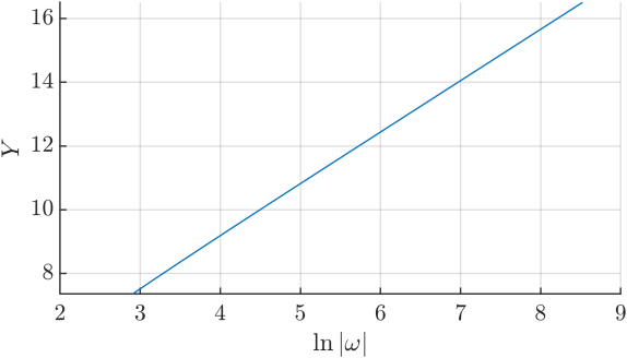
Figure 3: Points $(\ln|\omega|,Y_{\Delta\dot{\mathpzc}x})$ varying (decreasing to zero) $K$ (or equivalently increasing $\ln|\omega|$). Notice the points lying on the line $Y=2.772+1.6115\ln|\omega|$.

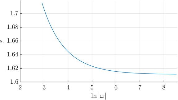
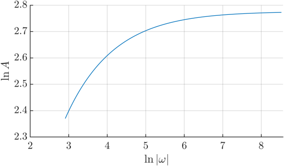
Figure 4: Values of $r$ (left) and $\ln A$ (right) obtained when taking pairs of points $(K_{i},\Delta\dot{\mathpzc}x_{i})$ and $(K_{i+1},\Delta\dot{\mathpzc}x_{i+1})$ varying (decreasing to zero) $K$ (or equivalently increasing $\ln|\omega|$). See the text for details.

(iii) Actually, a more precise version of formula (39) can be written as

$$\Delta\dot{\mathpzc}x\sim\varepsilon|\omega|^{r}\exp\left(\frac{w\pi}{2}\right)\left(A+A_{1}\varepsilon^{j_{1}}+A_{2}\varepsilon^{j_{2}}+\cdots\right)$$

or equivalently as

$$Z_{\Delta\dot{\mathpzc}x}:=\frac{1}{\varepsilon}|\omega|^{-r}\Delta\dot{\mathpzc}x\exp\left(-\frac{\omega\pi}{2}\right)\sim A+A_{1}\varepsilon^{j_{1}}+A_{2}\varepsilon^{j_{2}}+A_{3}\varepsilon^{j_{3}}+\cdots$$ (41)

and our goal is to obtain an (as much precise as possible) value of $A$, once $r$ is given. Although we do not know the exact value of $r$, from the numerical computations done in next Sections for the perturbed pendulum and for the perturbed amended pendulum, we will show (later on) that the guess value for $r$ is $r=1.611111\ldots=29/18$.

Using formula (41) we have done several steps of extrapolation to obtain a robust value of $A$ (using the last 50 values of $K$ close to $10^{-8}$) (see values of $(K,\varepsilon)$ in Table 1, where only the smallest 10 values of K are shown). That is, we have taken values of $(\varepsilon,Z_{\Delta\dot{\mathpzc}x})$ (see column 2 and 3 in the table) and after some attempts, varying the values of $j_{i}$, we conclude that we get the best fit of $A$ with $j_{i}=2\cdot i$ and the value of $A$ is $A=16.055307843$ (or $\ln A=2.776039450$). See columns 3, 4, 5 in the table. Columns 4 and 5 have been obtained taking the first two extrapolation steps.

$K$	$\varepsilon$	$Z_{\Delta\dot{\mathpzc}x}$	1st extrapolation	2nd extrapolation
1.432E-8	8.312E-3	16.0493664120828	16.05530749436553	16.0553078439006
1.419E-8	8.293E-3	16.0493937101860	16.05530749756964	16.0553078438344
1.406E-8	8.274E-3	16.0494208816007	16.05530750074373	16.0553078437819
1.393E-8	8.255E-3	16.0494479266667	16.05530750388795	16.0553078437170
1.380E-8	8.236E-3	16.0494748478517	16.05530750700268	16.0553078436392
1.367E-8	8.217E-3	16.0495016497992	16.05530751008853	16.0553078435483
1.355E-8	8.198E-3	16.0495283244532	16.05530751314551	16.0553078433730
1.342E-8	8.179E-3	16.0495548764688	16.05530751617363	16.0553078434478
1.330E-8	8.160E-3	16.0495813084435	16.05530751917351	16.0553078433717
1.318E-8	8.141E-3	16.0496076165450	16.05530752214528	16.0553078433357

Table 1: Approximate values of $A$ in formula (41) obtained by extrapolation.

In summary, with the data at hand the specific values of $A$ and $r$ turn out to be

$$A=16.055307843\dots,\qquad r=1.6111111\ldots=29/18.$$ (42)

3.3 Splitting in resonant coordinates

Motivated, on one hand, by formulas (34) and (33) at $t=0$ which provide explicit expressions of the splitting for the perturbed pendulum, and on the other hand, by the numerical simulations done in the previous subsection, we want to analyse the splitting (distance between the external manifolds $W^{u,e}$ and $W^{s,e}$ at the Poincaré section $\Sigma$) when taking into account, not the original variables $(\mathpzc x,\mathpzc y,\mathpzc p_{\mathpzc x},\mathpzc p_{\mathpzc y})$ but the resonant ones $(x,y,p,q)$. So, for each value of $K$, once we obtain the point $P^{u}$ from the computations described in the previous subsection for the CP problem, we apply the change of coordinates from Levi-Civita $(u,v,u^{\prime},v^{\prime})$ to synodical ones $(\mathpzc x,\mathpzc y,\mathpzc p_{\mathpzc x},\mathpzc p_{\mathpzc y})$ and to resonant coordinates $(x,y,p,q)$, so now $P^{u}$ becomes $(x^{u},y^{u},q^{u},p^{u})$, with $x^{u}\approx\pi$. Taking the same range of values of $K$ tending to zero, more precisely a set of values $K_{i}$, $i=1,\dots,N$ with $K\in[10^{-8},10^{-3}]$ and using multiple precision computations, we compute the splitting which now we define as $\Delta p=2p^{u}$. (notice that it is not $p^{u}-p^{s}$, since $x$ is not exactly equal to $\pi$). Taking into account formulas (33) and (34), where we skip the $+$ notation since we only consider the external manifolds, we fit the splitting by the asymptotic formula

$$\Delta p\sim\varepsilon\bar{A}|\omega|^{\bar{r}}\exp\left(\frac{\omega\pi}{2}\right)$$ (43)

or equivalently

$$\ln|\Delta p|-\ln\varepsilon-\frac{\omega\pi}{2}\sim\ln\bar{A}+\bar{r}\ln|\omega|.$$ (44)

Our next goal is to determine $\bar{A}$ and $\bar{r}$. We proceed applying the three strategies mentioned above.

(i) We plot the points $(\ln|\omega|,Y_{\Delta p})$, with $Y_{\Delta p}:=\ln|\Delta p|-\ln\varepsilon-\dfrac{\omega\pi}{2}$, see Figure 5. Again we observe the good fit of points $(\ln|\omega|,Y_{\Delta p})$ by a line. A linear regression approximation using formula (44) provides $\ln\bar{A}=3.325$ and $\bar{r}=2.111$.

(ii) Taking each successive pair of points $(K_{i},\Delta p_{i})$ and $(K_{i+1},\Delta p_{i+1})$ and the segment passing through the points $(\ln|\omega_{i}|,Y_{\Delta p_{i}})$ and $\left(\ln|\omega_{i+1}|,Y_{\Delta{p_{i+1}}}\right)$. We associate to this segment the expression $\bar{r}\ln|\omega|+\ln\bar{A}$ and we plot the obtained values of $\bar{r}$ in Figure 6 left and the obtained values of $\ln\bar{A}$ in the right figure. With the data at hand, the last values obtained for $\ln\bar{A}$ and $\bar{r}$ are $\ln\bar{A}=3.323854\dots$, $\bar{r}=2.111267\dots$, which are very similar to those values in strategy (i).

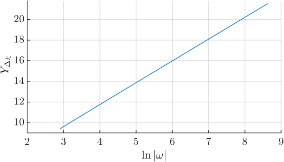
Figure 5: Points $(\ln|\omega|,Y_{\Delta p})$ varying (decreasing to zero) $K$ (or equivalently increasing $\ln|\omega|$). Notice the points lying on the line $Y=3.325+2.111\ln|\omega|$.

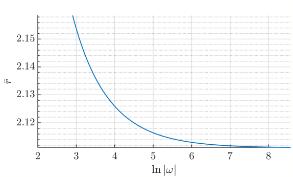
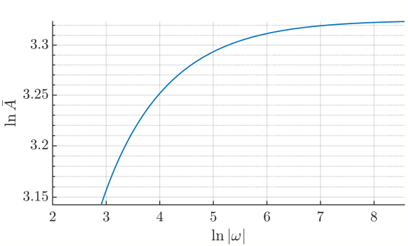
Figure 6: Values of $\bar{r}$ (left) and $\ln\bar{A}$ (right) obtained when taking pairs of points $(K_{i},\Delta p_{i})$ and $(K_{i+1},\Delta p_{i+1})$, in resonant coordinates, varying (decreasing to zero) $K$ (or equivalently increasing $\ln|\omega|$). See the text for details.

(iii) We now make use of the fit formula

$$\Delta p\sim\varepsilon|\omega|^{\bar{r}}\exp\left(\frac{\omega\pi}{2}\right)\left(\bar{A}+\bar{A}_{1}\varepsilon^{j_{1}}+\bar{A}_{2}\varepsilon^{j_{2}}+\dots\right),$$

or equivalently as

$$Z_{\Delta p}:=\frac{1}{\varepsilon}|\omega|^{-\bar{r}}\Delta p\exp\left(-\frac{\omega\pi}{2}\right)\sim\bar{A}+\bar{A}_{1}\varepsilon^{j_{1}}+\bar{A}_{2}\varepsilon^{j_{2}}+\bar{A}_{3}\varepsilon^{j_{3}}+\dots$$ (45)

and as we have done previously with $\Delta\dot{x}$, we want to apply extrapolation to obtain an (as much precise as possible) value of $\bar{A}$, once $\bar{r}$ is given. Again, we need a guess value which turns out to be $\bar{r}=2.11111\ldots=19/9$. This value will be justified in Section 5.

Using formula (45) we have done two steps of extrapolation to obtain a robust value of $\bar{A}$ (again using the same last $50$ values of $K$ close to $10^{-8}$, see Table 2) where we have taken $j_{i}=2\cdot i$ (which provides the best fit). We list the values of $\bar{A}$ obtained through the successive extrapolation steps (we only provide the last 10 values but we have used $50$):

$Z_{\Delta p}$	1st extrapolation	2nd extrapolation
27.8040812616518	27.80860932094579	27.8086089167525
27.8041020671644	27.80860931723887	27.8086089166344
27.8041227760921	27.80860931356489	27.8086089165020
27.8041433886943	27.80860930992373	27.8086089163859
27.8041639068522	27.80860930631499	27.8086089162863
27.8041843341052	27.80860930273799	27.8086089162036
27.8042046643138	27.80860929919275	27.8086089160301
27.8042249010261	27.80860929567928	27.8086089159491
27.8042450462224	27.80860929219689	27.8086089158544
27.8042650969822	27.80860928874547	27.8086089157148

Table 2: Approximate values of $\bar{A}$ in formula (45) obtained by extrapolation.

In summary, with the data at hand, the values of $\bar{A}$ and $\bar{r}$ turn out to be

$$\bar{A}=27.80860891\dots\quad(\ln\bar{A}=3.325345645\dots),\qquad\bar{r}=2.11111\ldots=19/9,$$ (46)

Remark We notice that the Poincaré section $y=0$ does not correspond to $x=\pi$ but $x=\pi+\delta$. However, numerical computations reveal that

$$\delta=C\varepsilon^{2}|\omega|^{\bar{r}}\exp\left(\frac{\omega\pi}{2}\right)$$

so in terms of comparison of the fit formulas for the splitting, we can deal with the Poincaré section $x=\pi$ or $x=\pi+\delta$, indistinctly (since the contributionn of $\delta$ is of order $\varepsilon^{2}$, apart from the exponentially small term).

At this point, two natural questions arise: (i) Can we explain the difference between $r=1.611\dots$ and $\bar{r}=2.111\dots$? (ii) Does the Melnikov theory predict the asymptotic formula (43) or (44) with these values of $\bar{r}$ and $\ln\bar{A}$?

Next section is devoted, in particular, to answer the second question.

Concerning the first question let us prove the following result:

At the Poincaré section $\Sigma:\quad\mathpzc y=0$, we have

$$\dot{\mathpzc}x\approx\varepsilon p$$

or equivalently

$$\Delta\dot{\mathpzc}x\approx\varepsilon\Delta p.$$

To prove this assertion, let us assume that $\mathpzc x=1+O(\delta)$, $\dot{\mathpzc}y=O(\delta)$, and $\dot{\mathpzc}x>0$ being $\delta$ a small quantity. Then

$$a =\frac{\mathpzc x}{2-\mathpzc x(\dot{\mathpzc}x^{2}+\dot{\mathpzc}y^{2})-2\dot{\mathpzc}y\mathpzc x^{2}-\mathpzc x^{3}}=\frac{1+O(\delta)}{2-(1+O(\delta))(\dot{\mathpzc}x^{2}+O(\delta^{2}))-2O(\delta^{2})-1+O(\delta)}$$

$$=\frac{1+O(\delta)}{1-\dot{\mathpzc}x^{2}(1+O(\delta))+O(\delta)}=\frac{1+O(\delta)}{1-\dot{\mathpzc}x^{2}+O(\delta)}$$

$$=\frac{1}{1-\dot{\mathpzc}x^{2}}+O(\delta),$$

$$L =\frac{1}{\sqrt{1-\dot{\mathpzc}x^{2}}}+O(\delta)$$

$$G =\mathpzc x(\dot{\mathpzc}y+\mathpzc x)=1+O(\delta)$$

so

$$L-G=\frac{\dot{\mathpzc}x^{2}}{\sqrt{1-\dot{\mathpzc}x^{2}}+1-\dot{\mathpzc}x^{2}}+O(\delta)$$

and

$$\sqrt{2(L-G)}=\frac{\sqrt{2}\dot{\mathpzc}x}{\sqrt{\sqrt{1-\dot{\mathpzc}x^{2}}+1-\dot{\mathpzc}x^{2}}}+O(\delta)$$

$$e=\sqrt{1-\frac{G^{2}}{a}}=\dot{\mathpzc}x+O(\delta).$$

Moreover the vector ${\bf e}=(e^{(1)},e^{(2)})$, with $e^{(2)}=-\mathpzc x\dot{\mathpzc}x(\dot{\mathpzc}y+\mathpzc x)=-\dot{\mathpzc}x+O(\delta)$. So finally

$$p=\frac{\sqrt{2(L-G)}}{\varepsilon}\sin g=\frac{\sqrt{2(L-G)}}{\varepsilon}\frac{e^{(2)}}{e}\approx\frac{1}{\varepsilon}\dot{\mathpzc}x,$$

that is

$$\dot{\mathpzc}x\approx\varepsilon p.$$ (47)

Expression (47) allows us to relate the exponent $r$ and $\bar{r}$ and the constants $A$ and $\bar{A}$ in the two fit formulas:

$$\dot{\mathpzc}x\sim A\varepsilon|\omega|^{r}\exp\left(\frac{w\pi}{2}\right),\quad r=1.61111\ldots=\frac{28}{19},$$ with

$$p\sim\bar{A}\varepsilon|\omega|^{\bar{r}}\exp\left(\frac{w\pi}{2}\right),\quad \bar{r}=2.1111\ldots=r+\frac{1}{2}=\frac{19}{9}.$$ with

Using $\dot{\mathpzc}x=\varepsilon p$, we obtain

$$\bar{r}=r+\frac{1}{2},\qquad A\approx\frac{\bar{A}}{\sqrt{3}}$$ (48)

which agrees with the relation $\bar{r}=2.11111\ldots=1.611111+0.5=r+0.5$ and if we compare the numerical values obtained

$$A=16.0553078\dots,\qquad\bar{A}=27.8086089\dots$$

we precisely get $\frac{\bar{A}}{\sqrt{3}}=16.0553078\dots$ which coincides with the value of $A$ up to the first 9 digits.

4 The perturbed pendulum. Other possible models

This Section is devoted to answer the following question: does the Melnikov theory predict the asymptotic formula (43) with these values of $\bar{r}$ and $\ln\bar{A}$?

To answer this question we take, as the most natural model, the first order in $\varepsilon$ Hamiltonian. More precisely, in Section 2.3 we have written the Hamiltonian of the CP problem in resonant coordinates $(x,y,q,p)$ (see (16)). We now consider the Hamiltonian as an expansion in powers of $\varepsilon=\left(K/3\right)^{1/4}$:

$$H =\omega\frac{q^{2}+p^{2}}{2}+\frac{y^{2}}{2}+\cos x-1+\varepsilon\left[\frac{3}{2}q-\frac{q}{2}\cos 2x-\frac{p}{2}\sin 2x\right]$$

$$\quad+\varepsilon^{2}\left[\left(-\frac{3}{8}q^{2}-\frac{5}{8}p^{2}\right)\cos x+2y\cos x+\frac{1}{4}qp\sin x+\frac{3}{8}\left(q^{2}-p^{2}\right)\cos 3x+\frac{3}{4}qp\sin 3x-\frac{2}{3}y^{3}\right]+\cdots$$

$$:=H_{0}+\varepsilon H_{1}+\varepsilon^{2}H_{2}+\cdots$$ (49)

and we take as the simplest model the first order expansion,

$$\hat{H}(x,y,q,p)=H_{0}(x,y,q,p)+\varepsilon H_{1}(x,y,q,p)$$ (50)

with

$$H_{0}(x,y,q,p)=\omega\frac{q^{2}+p^{2}}{2}+\frac{y^{2}}{2}+\cos x-1$$ (51)

and

$$H_{1}(x,y,q,p)=\frac{3}{2}q-\frac{q}{2}\cos 2x-\frac{p}{2}\sin 2x,$$ (52)

and we call (50) the perturbed pendulum (although $H_{0}$ is a rotor times a pendulum).

We want to test the Melnikov theory (that is, to check if the Melnikov integral (30) and (33) using Hamiltonian (50) predicts the asymptotic behavior for the splitting provided by (43) or (44)). A clear advantage of this Hamiltonian is that we know the explicit expression of the separatrices (given by (20)) in $(q,p)=(0,0)$ of the integrable Hamiltonian $H_{0}(x,y,q,p)$, which is a rotor times a pendulum. We observe that the associated system of ODE to $\tilde{H}$ has two equilibrium points: $L_{-}=(0,0,3\varepsilon^{3},0)$ and $L_{+}=(2\pi,0,3\varepsilon^{3},0)$. We will focus our attention on the external unstable manifold of $L_{-}$ (that will start describing a curve in the $(x,y)$ projection with $y>0$, $x>0$), and the external stable manifold of $L_{+}$ (that will start describing a curve in the $(x,y)$ projection with $y>0$, $x<2\pi$). We want to measure the distance between them (the splitting) at a given Poincaré section. Due to the symmetry $(x,y,q,p,t)\to(2\pi-x,y,q,-p,-t)$ satisfied by the associated system of ODE, a Poincaré section that turns out to be convenient is $x=\pi$, $y>0$. From now on we will omit the external mention when discussing the manifolds and we will simply refer to them as the manifolds.

4.1 Melnikov integral for the perturbed pendulum

Formula (34) provides the Melnikov integral for the separatrix of the pendulum and Formula (32) provides (the linear approximation of) the splitting. In particular at $t=0$ we have

$$\Delta p\sim-\varepsilon^{m}\frac{8\pi}{3}\omega^{3}\left(1-\frac{2}{\omega^{2}}\right)\frac{\ee^{\pi\omega/2}}{1-\ee^{2\pi\omega}},$$ (53)

with $m=1$. So, comparing the splitting fit formulas (43) and (53) we obtain $\bar{r}=3$ from Melnikov formulation, instead of the expected value $\bar{r}=2.111\dots$ and $\bar{A}=\frac{8\pi}{3}=8.377\dots$ instead of $\bar{A}=27.808\dots$ (see (46)). We can conclude that the numerical results for $\Delta p$ do not coincide with the theoretical prediction given by the Melnikov formula.

4.1.1 Analysis of the Toy CP problem with $a=0$

Although the Hamiltonian $\hat{H}$ in (50) turns out not to be a good approximation to get the asymptotic fit for $\Delta p$ for the CP problem, it is interesting to analyze the following Hamiltonian—per se and to compare our results with previous ones in the literature—, taking the same integrable part plus a more general perturbation, that is the Toy CP problem with $a=0$,

$$\tilde{H}(x,y,q,p)=H_{0}(x,y,q,p)+\varepsilon^{m}H_{1}(x,y,q,p)$$ (54)

where $m\geq 1$, $H_{0}$ and $H_{1}$ are given by (51) and (52). Let us note first that there are theoretical results [1, 5] for Hamiltonian systems with $1+\nicefrac{{1}}{{2}}$ degrees of freedom that can be directly applied to the Toy CP problem with $a=0$ (54). According to these theoretical results, for $m\geq 4$ the Melnikov prediction with the standard pendulum gives the correct measure (53) for the splitting.

Let us consider the equilibrium points of $\tilde{H}$, $L_{-}=(0,0,3\varepsilon^{2+m},0)$ and $L_{+}=(2\pi,0,3\varepsilon^{2+m},0)$. Our goal, in this subsection, is to check if the splitting between the unstable manifold of $L_{-}$ (in $y\geq 0$) and the stable manifold of $L_{+}$ (in $y\geq 0$) measured at the Poincaré section $\tilde{\Sigma}$ defined by $x=\pi$, $y>0$ can be predicted by the Melnikov formula (31) obtained analytically regardless the value of $m$.

To do so, we fix a value of $m$, and for each value of $K$ (or equivalently $\varepsilon$ or $\omega$):

1. We compute the associated equilibrium point $L_{-}=(0,0,3\varepsilon^{2+m},0)$ of the corresponding Hamiltonian system.

2. We compute, using the parameterization method and multiple precision arithmetics, the unstable manifold $\Cu(L_{-})$ up to the Poincaré section $\widetilde{\Sigma}$. We call $(x^{u},y^{u},q^{u},p^{u})$ the corresponding point with $x^{u}=\pi$.

3. We would proceed similarly with the stable manifold of $L_{+}$ and we would compute the intersection point $(x^{s},y^{s},q^{s},p^{s})$ with $\widetilde{\Sigma}$. However, due to the symmetry

$$(x,y,q,p,t)\to(2\pi-x,y,q,-p,-t)$$ (55)

only the unstable manifold $\Cu(L_{-})$ needs to be computed since at the Poincaré section we have $x^{u}=x^{s}=\pi$, $q^{u}=q^{s}$, $p^{u}=-p^{s}$ and $y^{u}=y^{s}$. We are interested in the splitting between $\Cu(L_{-})$ and $\Cs(L_{+})$ at $\widetilde{\Sigma}$, that is, the value

$$\Delta p=p^{u}-p^{s}=2p^{u}$$

4. We vary the values of $K$ tending to 0 (or $\varepsilon$ or $\omega$), and we obtain a set of points $(K_{i},\Delta p_{i})$, for $i=1,\dots,N$. In the numerical simulations we have taken decreasing values of $K$ up to $3\cdot 10^{-8}$. Again order of thousands for the parametrization and multiple precision with thousands of digits are required.

5. We fit the numerical computed values by a formula of type,

$$\Delta p\sim\varepsilon\tilde{A}|\omega|^{\tilde{r}}\cdot\exp\left(\frac{\omega\pi}{2}\right)$$ (56)

or equivalently,

$$\ln|\Delta p|-\ln\varepsilon-\frac{\omega\pi}{2}\sim\ln\tilde{A}+\tilde{r}\ln|\omega|.$$

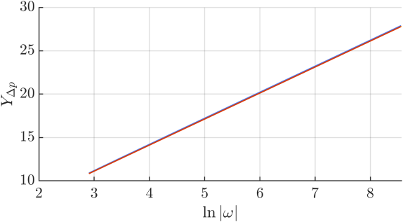
Figure 7: Points $(\ln|\omega_{i}|,Y_{\Delta p_{i}})$ for $m=1,2,3,4,5,6$. Notice they overlap on a line.

Let us discuss the results obtained. Notice that we want to check two different values: the exponent $\tilde{r}$ which should be equal to $3$ and the constant $\tilde{A}$ which should be $8\pi/3$ or $\ln\tilde{A}=2.125591\dots$. In Figure 7 we show a first (rough) plot with the points $(\ln|\omega_{i}|,Y_{\Delta p_{i}})$ with $Y_{\Delta p_{i}}:=\ln|\Delta p_{i}|-\ln\varepsilon_{i}-\omega_{i}\pi/2$ (and $\varepsilon_{i}=(K_{i}/3)^{1/4}$ and $\omega_{i}=-1/(3\varepsilon_{i}^{2})$), where we have taken some values of $K$ ranging from $0.005$ to $5\cdot 10^{-8}$. Taking such a big set of values of $K$ for each value of $m$, we can see how the set of points for each case $m=1,2,3,4,5,6$ overlap on the line $Y=2.1255+3\ln|\omega|$.

However, formula (56) is an asymptotic formula, so to find out the tendency of $\tilde{r}$ towards $3$ and $\ln A$ towards $\ln(8\pi/3)=2.1255\dots$ (see the dashed horizontal line in Figures 8 and 10), we proceed as above, that is, we compute, for each two successive points $(\ln|w_{i}|,Y_{\Delta p_{i}})$ and $(\ln|w_{i+1}|,Y_{\Delta p_{i+1}})$, the segment passing through these two points, with an expression $\tilde{r}_{i}\ln|w|+\ln\tilde{A}_{i}$. Taking values of $K$ decreasing from $0.005$ to $5\cdot 10^{-8}$, we plot the set of points $(\ln|w_{i}|,\tilde{r}_{i})$, $i=1,\dots,N-1$, in Figure 8 left and $(\ln|w_{i}|,\ln\tilde{A}_{i})$, $i=1,\dots,N-1$, in Figure 8 right. These computations are shown for $m=1,2,3,4,5,6$. Some remarks must be mentioned:

(i) it is clear that the value of $\tilde{r}$ tends to $3$ for the values of $m$ considered so the exponent 3 in the theoretical Melnikov formula (32) fits with the numerical exponent obtained. Moreover we also observe that for $m=2,3,4,5,6$ (say $m\geq 2$) the tendency of $\tilde{r}$ is mainly the same and fast towards the value $3$, but for $m=1$ it takes a bit longer to tend to $3$. But in all cases, $\tilde{r}$ tends to $3$ when $K$ tends to zero. So we may infer that for any $m\geq 1$, the exponent $\tilde{r}$ is 3.

(ii) Concerning the value of the constant $\ln\tilde{A}$, it is clear that, for $m\geq 2$, $\ln\tilde{A}\to\ln(8\pi/3)$. However, in principle it is not that clear for $m=1$. Another way to show the tendency of $\tilde{r}_{i}$ and $\ln\tilde{A}_{i}$ to $3$ and $\ln(8\pi/3)=2.1255\dots$ respectively, is based on the computation of the points $(\ln|w_{i}|,|\tilde{r}_{i}-3|)$ in Figure 9 left and the points $(\ln|w_{i}|,|\ln\tilde{A}_{i}-\ln(8\pi/3)|)$ in Figure 9 right. We see in the left figure that for $m=3,4,5,6$ the points overlap on the same curve and $|\tilde{r}-3|$ tends clearly to zero. In particular, for $m=2$, the curve $\tilde{r}$ crosses the value $\tilde{r}=3$. See Figure 8 left (i.e. the points on the curve $(\ln|w|,|\tilde{r}-3|)$ describe a sharp minimum for a value of $\ln|w|$ close to 5 and the values of $\tilde{r}$ tend to 3) and we observe the decreasing tendency to zero in Figure 9 left). We also see the decreasing tendency to zero for $m=1$, but not as fast as the one for $m=2$ or $m\geq 3$.

Similarly, looking at the Figure 9 right, we observe for $m=3,4,5,6$ the fast tendency of

$$\left|\ln\tilde{A}-\ln\left(\frac{8\pi}{3}\right)\right|$$

to zero. However for $m=2$, the curve $|\ln\tilde{A}|$ (see Figure 8 right) crosses the value $\ln(8\pi/3)$ (it is clearly seen in the sharp minimum for $|\ln\tilde{A}-\ln(8\pi/3)|$ in Figure 9 right), has a local maximum and goes on decreasing tending to $\ln(8\pi/3)$ (we observe a slower tendency to zero in Figure 9 right). Similarly we expect this to happen for $m=1$. Actually we see the crossing value $\ln(8\pi/3)$, and (almost) the maximum. However we cannot observe the decreasing tendency to $\ln(8\pi/3)$ as expected. We conjecture that this is the case.

To support this conjecture, the previous computation naturally leads to explore the behavior of $\tilde{r}$ and $\ln\tilde{A}$ for intermediate values of $m$ between 1 and 2, to see the continuous evolution. This has been done for $m=1.1,1.2,1.3,\dots,1.9$ and we show the results in Figure 10 left for $\tilde{r}$ and right for $\ln\tilde{A}$. We notice the continuous evolution of the curves for the intermediate different values of $m$. In particular, on the left plot we see the tendency of $\tilde{r}$ to $3$ for any value of $m$. On the right plot we see the maximum in each curve $\ln\tilde{A}$ for $m=1.1,\dots,1.9$ and the asymptotic tendency to $2.1255\dots$, as $\ln|w|$ increases, however for $m=1$ we see the maximum but not the expected decreasing tendency to $2.1255\dots$. To do so, we should consider smaller values of $K$. But this becomes numerically unfeasible (to compute the value of $\Delta p$ for $K=5\cdot 10^{-8}$ we need thousands of digits and an order of thousands for the parametrization of the manifold, so smaller values of $K$ become prohibitive).

6. A double check concerning the value of $\tilde{A}$ is related to the extrapolation procedure done in Subsection 3.3. More precisely, for every value of $m\geq 1$ fixed, we apply (finite) extrapolation steps to the first fit formula:

$$\frac{\Delta p|\omega|^{-\tilde{r}}\exp\left(-\dfrac{\omega\pi}{2}\right)}{\varepsilon^{m}}\sim\tilde{A}+\tilde{A}_{2}\varepsilon^{2}+\tilde{A}_{4}\varepsilon^{4}+\cdots$$

or to the second fit formula

$$\frac{\Delta p|\omega|^{-\tilde{r}}\exp\biggl{(}-\dfrac{\omega\pi}{2}\biggr{)}}{\varepsilon^{m}\left(1-\dfrac{2}{\omega^{2}}\right)}\sim\tilde{A}+\bar{\tilde{A}}_{2}\varepsilon^{2}+\bar{\tilde{A}}_{4}\varepsilon^{4}+\cdots$$

both formulas with $r=3$. We also want to compare both formulas and to check if the second one somewhat improves the first one.

Our simulations show that, as $m$ increases, the number of digits obtained for the value of $\tilde{A}=8\pi/3$ also increases when taking the second fit formula instead of the first one. For example, for $m=6$ we obtain, respectively, 6, 10 digits when taking a first step and a second step of extrapolation using the first fit formula, whereas we obtain 20, 20 digits with two successive steps of extrapolation applied to the second fit formula. However, as $m$ decreases, for example $m=1$, neither the first nor the second fit formula, even using extrapolation, are able to provide good digits of $\tilde{A}$. As mentioned above, we should need smaller values of $K$, which is not feasible.

So, from the numerical simulations, we can conclude that for the Toy CP problem with $a=0$, Hamiltonian (54),

(i) formula (56) provides a good fit formula for the splitting $\Delta p$, and

(ii) the Melnikov formula predicts the splitting for any $m>1$ both in $\tilde{r}$ and $\tilde{A}$. However for $m=1$, while the tendency of $\tilde{r}$ to $3$ is clear, we conjecture this tendency to happen for $\ln\tilde{A}$ to $2.1255\dots$ but the numerical results are not conclusive enough.

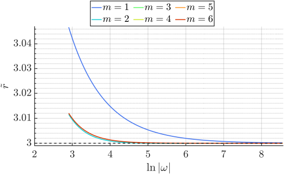
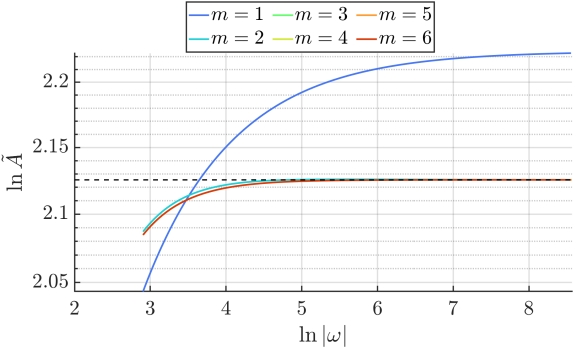
Figure 8: The perturbed pendulum. Points $(\ln|\omega|,\tilde{r})$ (left), and $(\ln|\omega|,\ln\tilde{A})$ (right) obtained for $m=1,\ldots,6$. The dashed line (on the right figure) corresponds to the value $\ln(8\pi/3)=2.1255\dots$.

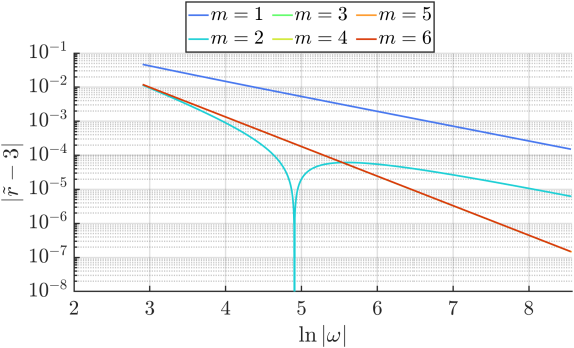
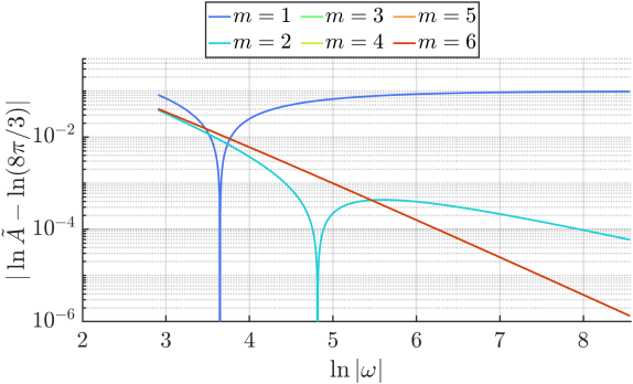
Figure 9: The Toy CP problem with $a=0$. Points $(\ln|\omega|,|\tilde{r}-3|)$ (left), and $(\ln|\omega|,|\ln\tilde{A}-\ln(8\pi/3)|)$ (right) obtained for $m=1,\ldots,6$.

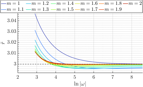
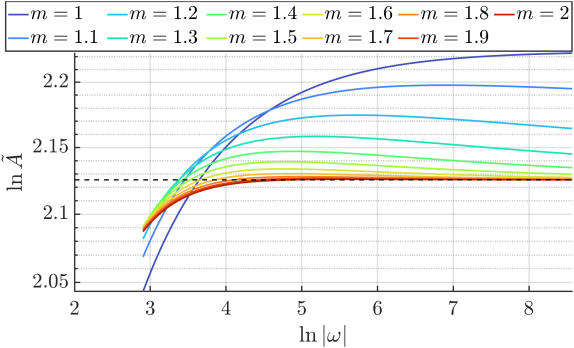
Figure 10: The Toy CP problem with $a=0$. Points $(\ln|\omega|,\tilde{r})$ (left), and $(\ln|\omega|,\ln\tilde{A})$ (right) obtained for $m=1,1.1,\ldots,2$. The dashed line (on the right figure) corresponds to the value $\ln(8\pi/3)=2.1255\dots$.

4.2 Other strategies/models to fit the numerical computation of $\Delta p$ for the CP problem

Recall that our purpose is to find a simplified model that mimics the splitting $\Delta p$ of the CP problem in resonant coordinates. And we have just shown that the perturbed pendulum, $H=H_{0}+\varepsilon H_{1}$, is not good enough.

So we want to find out another simple model that does describe the splitting of the CP problem.

A natural procedure is to take the second order approximation

$$H=H_{0}+\varepsilon H_{1}+\varepsilon^{2}H_{2}$$

see (4), and consider different truncated Hamiltonians adding to $H_{0}+\varepsilon H_{1}$ different terms of $\varepsilon^{2}H_{2}$. For each selected Hamiltonian, we, first, take a value of $K$ and we compute the splitting $\Delta p$ (obtained from the intersection of the unstable manifold of the corresponding equilibrium point and the section $x=\pi$, $y>0$). Second, we repeat the procedure for different decreasing values of $K$ and, third, we fit $\Delta p$ by an expression of the type

$$\Delta p\sim\varepsilon\hat{A}|\omega|^{\hat{r}}\cdot\exp\left(\frac{\omega\pi}{2}\right)$$

and we want to know which terms of the Hamiltonian are relevant that give rise to a value of $\hat{r}$ equal to the one obtained for the CP problem, that is $\bar{r}=2.111\ldots=19/9$. We have done the numerical computations considering different truncated Hamiltonians taking different terms of $H_{2}$. We have used just quadruple precision and decreasing values of $K$ ranging from $0.001$ to $5\cdot 10^{-5}$ to have a first insight. From these numerical simulations we can conclude that the simplest model that reproduces the value of $\bar{r}=2.111\dots$ for the fitting splitting formula is the Hamiltonian provided by $H_{0}+\varepsilon H_{1}-(2/3)\varepsilon^{2}y^{3}$, that is, only the term $-(2/3)\varepsilon^{2}y^{3}$ in $H_{2}$ is responsible for changing the exponent $\tilde{r}=3$ (obtained from the perturbed pendulum) to $\bar{r}=2.1111\dots$.

So, in next Section we will consider this precise Hamiltonian and we will use multiple precision computations in order to show that we really obtain the value $\bar{r}=2.1111\ldots=19/9$.

5 The Toy CP problem with $a=1$

The previous discussion motivates to analyse the new Hamiltonian adding the term $(-2/3)\varepsilon^{2}y^{3}$ to the integrable part $H_{0}$ giving rise to a new integrable part,

$$\breve{H}_{0}(x,y,q,p)=H_{0}(x,y,q,p)-\frac{2}{3}\varepsilon^{2}y^{3},$$ (57)

which we will call amended pendulum, plus the perturbation, that is

$$\breve{H}_{0}(x,y,q,p)+\varepsilon H_{1}(x,y,q,p),$$

called from now on the perturbed amended pendulum. Or, more generally, we consider the Toy CP problem with $a=1$ and $m\geq 1$

$$\breve{H}(x,y,q,p)=\breve{H}_{0}(x,y,q,p)+\varepsilon^{m}H_{1}(x,y,q,p),$$

In this Section we will carry out two kind of computations:

(i) the computation of the Melnikov integral for $\Delta p$ (see formulas (30) and (33)). In this case, however, we cannot compute the Melnikow integral for the amended pendulum analytically (as we did for the pendulum) since no parametrisation of the homoclinic loop (the separatrices), for the integrable part $\breve{H}_{0}$, is available. So the Melnikov integral will be computed numerically. This will be done in Subsection 5.1.

(ii) The computation of the splitting $\Delta p$ (of the unstable and stable manifolds of the corresponding equilibrium points) at the Poincaré section $\widetilde{\Sigma}$. This will be done in Subsection 5.2.

(iii) Finally we will discuss the Melnikov prediction of the splitting for the Toy CP problem, on the one hand (in Subsection 5.2), and for the CP problem, on the other hand (in Subsection 5.3).

5.1 Numerical computation of the Melnikov formula using the amended pendulum

Recall formula (26) that provides the linear approximation of the splitting $\Delta v_{1}(t)=(\Delta q_{1}(t),\Delta p_{1}(t))$. We are interested in the splitting at $t=0$, so we use formula (33) for $\Delta v_{1}(0)=(\Delta q_{1}(0),\Delta p_{1}(0))$. In particular, for $H_{1}(x,y,q,p)$ in (28) we obtain

$$\Delta q_{1}(0)=0,\qquad\Delta p_{1}(0)=-\frac{1}{2}\int_{-\infty}^{\infty}\left(\cos\left(2x(t)+\omega t\right)-\cos\omega t\right)\>\!\!\df t,$$

where $(x(t),y(t))$ defines the separatrix of $\breve{H}_{0}$ and the right hand side term is precisely the Melnikov integral.

So an strategy to compute the Melnikov integral consists of integrating the system of ODE

$$\left\{\begin{aligned} \dot{x}&=y-2\varepsilon^{2}y^{2},\\ \dot{y}&=\sin x,\\ \dot{z}&=\cos(2x+\omega t)-\cos\omega t,\end{aligned}\right.$$ (58)

and more particularly the Melnikov integral

$$\frac{1}{2}\int_{-\infty}^{\infty}\left[\cos\left(2x+\omega t\right)-\cos\omega t\right]\>\!\!\df t=\int_{-\infty}^{0}\left[\cos\left(2x+\omega t\right)-\cos\omega t\right]\>\!\!\df t$$

due to the symmetry (55). So if $\displaystyle z(t)=\int_{-\infty}^{t}\dot{z}(u)\mathrm{d}u$ we want to compute the value $z(0)$.

We proceed with the following steps:

Step 1: Applying the parameterization method (see the Appendix) we obtain a local approximation of the unstable manifold (separatrix), $\bm{W}^{u}(\bm{0})$, associated with the equilibrium point $(0,0)$ of the system

$$\left\{\begin{aligned} \dot{x}&=y-2\varepsilon^{2}y^{2}\\ \dot{y}&=\sin x\end{aligned}\right.$$ (59)

that is, we have a (high order expansion of a) parametrization of the separatrix given by:

$$\sum_{k=1}^{N}\bm{w}_{k}s^{k}+O(s^{N+1})$$ (60)

Step 2: We compute a suitable value $\hat{s}$ small enough such that the error in this approximation is less than some given tolerance.

Step 3: We follow numerically the solution (the separatrix) of system (59) from the point

$$(x,y)=\sum_{k=1}^{N}\bm{w}_{k}\hat{s}^{k}$$

up to the section $\widetilde{\Sigma}$ ($x=\pi$) and compute the necessary time, $T$, to reach $\widetilde{\Sigma}$.

Step 4: We define $s_{0}=\cfrac{\hat{s}}{e^{-T}}$.

Step 5: We compute the integral of the function $z(t)$ from $-\infty$ to $-T$. To do so, we notice that from the Hamiltonian $\breve{H}_{0}$ in (57) and taking into account the value $H=h=0$ at $(0,0)$,

$$\cos x=1-\frac{y^{2}}{2}+\frac{2}{3}\varepsilon^{2}y^{3}$$

and we have

$$\dot{z}=\cos(2x+\omega t)-\cos\omega t=-2\dot{y}^{2}\cos\omega t+\dot{y}\left(-2+y^{2}-\frac{4}{3}\varepsilon^{2}y^{3}\right)\sin\omega t.$$ (61)

We notice that from (60) we have, in particular, the expansion of $y(t)$:

$$y(t)=y_{1}s_{0}e^{t}+y_{2}s_{0}^{2}e^{2t}+y_{3}s_{0}^{3}e^{3t}+\cdots=y_{1}s+2y_{2}s^{2}+3y_{3}s^{3}+\cdots$$

Thus, the expression of $\dot{z}$ in (61) becomes an expansion in $s$ (or equivalently in $s_{0}e^{t}$) together with the terms $\sin(\omega t)$ and $\cos(\omega t)$. We just need to integrate $\dot{z}(t)$ from $-\infty$ to $-T$. Let us provide a formula for the appearing terms in the integral:

$$\int_{-\infty}^{-T}a_{k}s^{k}\cos\omega t\>\!\df t =a_{k}\hat{s}^{k}\frac{k\cos(-\omega T)+\omega\sin(-\omega T)}{k^{2}+\omega^{2}},$$

$$\int_{-\infty}^{-T}a_{k}s^{k}\sin\omega t\>\!\df t =a_{k}\hat{s}^{k}\frac{k\sin(-\omega T)-\omega\cos(-\omega T)}{k^{2}+\omega^{2}}.$$

Step 6: Once we get the value $z(-T)=\displaystyle\int_{-\infty}^{-T}\!\!\dot{z}(t)\df t$ we integrate numerically system (58) from $-T$ to $0$, and we obtain $z(0)$.

Taking different decreasing values of $K$ from $K=0.001$ to $K=5.7\cdot 10^{-8}$, we fit the output values for the Melnikov integral by the formula

$$z(0)\sim\mathring{A}|\omega|^{\mathring{r}}\cdot\exp\left(\frac{\omega\pi}{2}\right)$$ (62)

or

$$\ln z(0)-\frac{\omega\pi}{2}\sim\mathring{r}\ln|\omega|+\ln\mathring{A},$$

and we obtain (see Figure 11)

$$\mathring{r}=2.111\dots,\qquad\qquad\ln\mathring{A}=2.279\dots.$$

We remark the good coincidence of the value of $\mathring{r}$ with that obtained for the CP problem in resonant coordinates $\bar{r}$.

Concerning the value of $\ln\mathring{A}$, there is not such coincidence with that obtained for the CP problem in resonant coordinates, $\ln\bar{A}$.

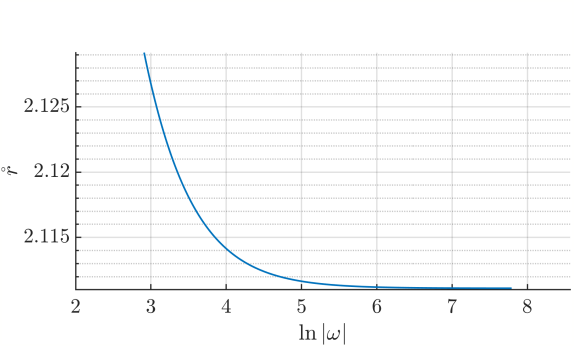
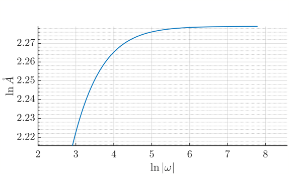
Figure 11: Curves $(\ln|\omega|,\mathring{r})$ and $(\ln|\omega|,\ln\mathring{A})$ obtained from the computation of the Melnikov integral.

5.2 Straight numerical computation of the splitting $\Delta p$

Similarly as we proceeded for the perturbed pendulum, we consider the Toy CP problem with $a=1$, that is,

$$\breve{H}(x,y,q,p)=H_{0}(x,y,q,p)-\frac{2}{3}\varepsilon^{2}y^{3}+\varepsilon^{m}H_{1}(x,y,q,p).$$

We fix a value of $m\geq 1$, we take different values of $K$ (decreasing up to $3\cdot 10^{-8}$), and for each $K$ given we compute the unstable manifold of the equilibrium point $L_{-}=(0,0,3\varepsilon^{2+m},0)$ intersection with $\widetilde{\Sigma}$ and we focus on the splitting $\Delta p=2p^{u}$, which we want to fit by

$$\Delta p\sim\varepsilon|\omega|^{\breve{r}}\exp\left(\frac{\omega\pi}{2}\right),$$ (63)

or equivalently

$$\ln\Delta p-m\ln\varepsilon-\frac{\omega\pi}{2}\sim\breve{r}\ln|\omega|+\ln\breve{A}$$ (64)

In this case, unlike the perturbed pendulum problem, we do not know neither the value of $\breve{r}$ nor the value of $\ln\breve{A}$ in formula (64).

We plot in Figure 12 left the obtained points $(\ln|\omega_{i}|,\breve{r}_{i})$ (similarly as we did above, that is, taking a segment between two successive points $(\ln|\omega_{i}|,Y_{\Delta p_{i}})$, $(\ln|\omega_{i+1}|,Y_{\Delta p_{i+1}})$, with $Y_{\Delta p}:=\ln\Delta p-m\ln\varepsilon-\omega\pi/2$). We observe the tendency of $\breve{r}$ towards the value $2.111115\dots$, which coincides with the value of $\mathring{r}$ obtained from the Melnikov integral.

Regarding the value of $\ln\breve{A}$, it is apparently clear that for $m\geq 2$, $\ln\breve{A}$ tends to $2.279\dots$, which coincides with the value of $\ln\mathring{A}$ obtained from the Melnikov integral. However it is not that clear for $m=1$. Analogously as we did for the perturbed pendulum, we now explore the intermediate values $m=1.1,1.2,1.3,1.4,\dots,1.9$ between $m=1$ and $m=2$. The results are shown in Figure 13 left –for $\breve{r}$– and right –for $\ln\breve{A}$–. The continuous evolution is clear. So we would expect, for $m=1$, a tendency of $\ln\breve{A}$ to $2.279\dots$. But again, as in the perturbed pendulum case, for $m=1$, we need smaller values of $K$ (which turns out to be prohibitive from a numerical point of view).

So, from the numerical computations done, we can conclude that for the Toy CP problem with $a=1$,

(i) the formula (64) provides a good fitting for $\Delta p$ with $\breve{r}=2.111\ldots=19/9$, for $m\geq 1$, and $\ln\breve{A}=2.279\dots$ for $m>1$, and we expect/conjecture also the same asymptotic value of $\ln\breve{A}$ for $m=1$.

(ii) The Melnikov integral does predict the value of the exponent $\mathring{r}=\breve{r}=19/9$ for $m\geq 1$ and the value of $\mathring{A}=\breve{A}=2.279\dots$ for $m>1$, and presumably also for $m=1$.

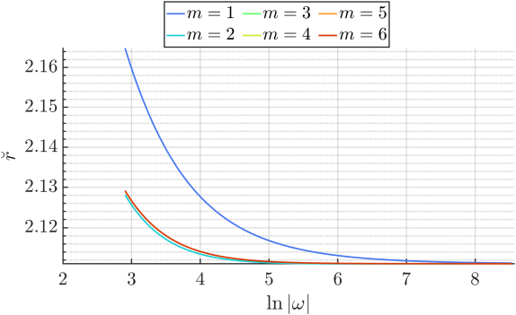
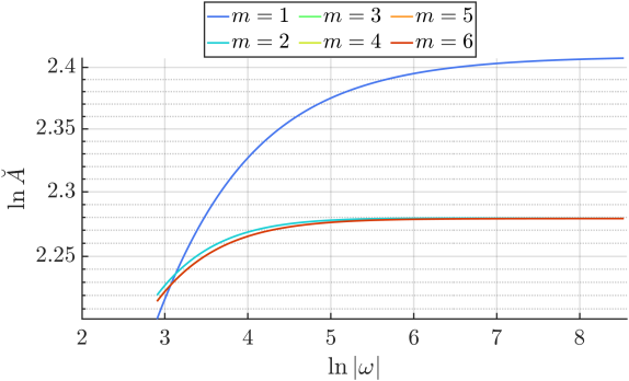
Figure 12: The Toy CP problem with $a=1$. Points $(\ln|\omega|,\breve{r})$ (left), and $(\ln|\omega|,\ln\breve{A})$ (right) obtained for $m=1,\ldots,6$.

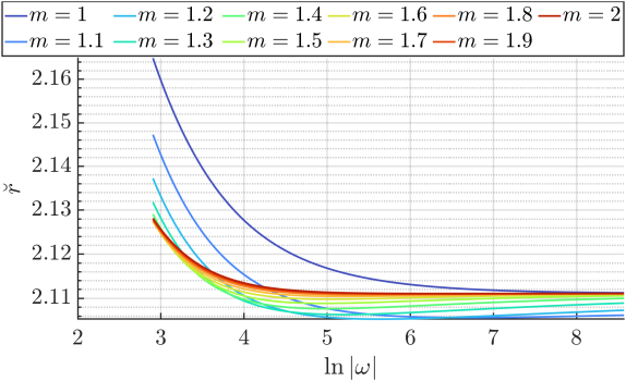
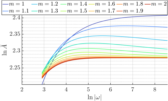
Figure 13: The Toy CP problem with $a=1$. Points $(\ln|\omega|,\breve{r})$ (left), and $(\ln|\omega|,\ln\breve{A})$ (right) obtained for $m=1,1.1,1.2,\ldots,2$

5.3 Agreement between the real CP problem and the Toy CP problem with $a=m=1$

(i) Concerning the computation of the splitting $\Delta p$ (from the unstable/stable manifolds at the intersection with $x=\pi$, $y>0$), we now consider two different problems: the original CP problem in resonant coordinates and the perturbed amended pendulum with $m=1$, that is, the Toy CP problem with $a=m=1$. We want to compare the respective values of $\bar{r}$ and $\breve{r}$ in the corresponding fit formulas (43) and (63).

More precisely, concerning the values of $\bar{r}$ and $\breve{r}$, we want to compare two curves, the numerical obtained curve, $(\ln|\omega|,\bar{r})$, for the splitting in resonant coordinates of the original CP Hamiltonian, and the numerical obtained curve, $(\ln|\omega|,\breve{r})$, for the splitting of the perturbed amended pendulum Hamiltonian (with $m=1$). In Figure 14 left we plot the curve $(\ln|\omega|,|\breve{r}-\bar{r}|)$ to find out the differences between both values. We remark the very good agreement of both values as far as $K$ decreases (or equivalently $\ln|\omega|$ increases).

So we can conclude that the perturbed amended pendulum is a simplified model that already describes the splitting of the CP problem, as far as asymptotic formulas (when $K$ tends to zero) are concerned.

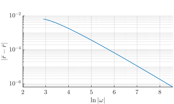
Figure 14: Curve $(\ln|\omega|,|\breve{r}-\bar{r}|)$ when computing the straight splitting from the CP problem and the perturbed amended pendulum (with $m=1$). See the text for details.

(ii) Finally, how does the Melnikov integral (taking into account the CP problem with $a=m=1$) predict the splitting for the CP problem in resonant coordinates? That is, we want to compare the fit formulas for $\Delta p$ (of the CP problem, that is (43)) and for the Melnikov integral (of the perturbed amended pendulum problem with $m=1$, that is (62)), more precisely, the values of the exponents $\bar{r}$ and $\mathring{r}$.

In Figure 15 we observe the difference $|\mathring{r}-\bar{r}|$ tending to zero. So we can conclude that the fitting asymptotic formula obtained for the Melnikov integral provides the same limit value of the exponent $\bar{r}=\mathring{r}=2.111\ldots=19/9$.

Remark. In Section 4, where we considered the perturbed pendulum, we discussed the known results (in the literature) compared with the ones obtained in this paper. However, for the Toy CP problem we are not aware of any published results.

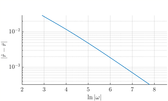
Figure 15: Curve $(\ln|\omega|,|\mathring{r}-\bar{r}|)$ when computing the straight splitting from the CP problem and the splitting using the Melnikov integral of the perturbed amended pendulum (with $m=1$). See the text for details.

Appendix A Computation of $\mathcal{A}^{\pm}\left(\omega\right)$

In this Appendix we explain how to derive the formula (34) that gives $\mathcal{A}^{\pm}(\omega)$ when $x_{0}(t)=x^{\pm}_{0}(t)$ is that of the standard pendulum given in (20). In particular we take $x_{0}(t)=x_{0}^{+}(t)$, so we consider the external branch ($y_{0}(t)=y_{0}^{+}(t)>0$). For the internal branch ($y_{0}(t)=y_{0}^{-}(t)<0$) the process that leads to $\mathcal{A}^{-}(\omega)$ can be carried out in a similar way, so we will not give the details here.

Let $(x^{\pm}_{0}(s),y^{\pm}(s))$ be the parameterization of the separatrices of the standard pendulum given in (20), and let $(x(s),y(s))$ denote specifically the external one, i.e.,

$$x_{0}(s)=x^{+}_{0}(s)=4\arctan\left(\mathrm{e}^{s}\right),\qquad y_{0}(s)=\dot{x}_{0}(s)=y^{+}_{0}(s)=\frac{2}{\cosh\>\!\!s}.$$

Following [15] we define

$$\mathcal{J}(a,b):=\int_{-\infty}^{\infty}\mathrm{e}^{\mathrm{i}as}\mathrm{e}^{\mathrm{i}b\tfrac{x_{0}(s)-\pi}{2}}y_{0}(s)\df s,$$ (65)

that, as it is pointed out there, is real whenever $a$ and $b$ are real. With the above definiton, integrating by parts the complex expression (29) of the real formula (34), it follows at once that

$$\mathcal{A}(\omega)=\int_{-\infty}^{\infty}\mathrm{e}^{\mathrm{i}\>\!\omega s}\left(1-\mathrm{e}^{2\mathrm{i}x_{0}(s)}\right)\!\df s=\left[\mathcal{Q}_{\omega}(r)\right]_{-\infty}^{\infty}+\frac{2}{\omega}\mathcal{J}(\omega,4),$$ (66)

where

$$\mathcal{Q}_{\omega}(r)=\frac{\mathrm{e}^{\mathrm{i}\omega r}}{\mathrm{i}\>\!\omega}\left(1-\mathrm{e}^{\mathrm{i}4\tfrac{x_{0}(r)-\pi}{2}}\right)=\frac{\mathrm{e}^{\mathrm{i}\omega r}}{\mathrm{i}\>\!\omega}\left[1-\left(\frac{1+\mathrm{i}\sinh r}{\cosh r}\right)^{4}\right],$$

so the “integrated” part at the rhs of (66) vanishes, since

$$\left[\mathcal{Q}_{\omega}(r)\right]_{-\infty}^{\infty}=\lim\limits_{r\to\infty}\mathcal{Q}_{\omega}(r)-\lim\limits_{r\to-\infty}\mathcal{Q}_{\omega}(r)$$

and clearly $\mathcal{Q}_{\omega}(r)\to 0$ as $r\to\pm\infty$. Hence, from (66), $\mathcal{A}(\omega)=2\mathcal{J}(\omega,4)/\omega$ and finally, we can use the formulas given in [15], Subsection 3.2, to compute (65) for $a=\omega$, $b=4$. Thus, after some algebra, it is seen that

$$\mathcal{A}(\omega)=\frac{2}{\omega}\mathcal{J}(\omega,4)=\frac{4}{3}\omega^{3}\left(1-\frac{2}{\omega^{2}}\right)\left[\frac{1}{\cosh\left(\dfrac{\pi\omega}{2}\right)}-\frac{1}{\sinh\left(\dfrac{\pi\omega}{2}\right)}\right]=\frac{16\pi}{3}\omega^{3}\left(1-\frac{2}{\omega^{2}}\right)\frac{\mathrm{e}^{\pi\omega/2}}{1-\mathrm{e}^{2\pi\omega}},$$

which is the equation (34) corresponding to $c^{\pm}=1$.

Appendix B Parameterization method

Let us assume that $z^{\ast}$ is a fixed point of the system $\dot{z}=F(z)$ with $F:\mathbb{R}^{n}\rightarrow\mathbb{R}^{n}$ regular enough. A simple strategy to compute an invariant manifold ($W$) associated with the point $z^{\ast}$ involves first calculating the tangent linear space to $W$ at $z^{\ast}$, i.e., $T_{z^{\ast}}W$. Points on $T_{z^{\ast}}W$ that are sufficiently close to $z^{\ast}$ can then be used as initial conditions for approximating $W$.

In this section, we focus specifically on computing the unstable manifold $W^{u}(z^{\ast})$, which we assume to be 1-dimensional. The computation for $W^{s}(z^{\ast})$ is analogous. Thus, we consider that $DF(z^{\ast})$ has a unique eigenvalue $\lambda>0$ with geometric multiplicity 1, and we denote its associated eigenvector by $v$.

A common strategy to compute a numerical approximation of the unstable invariant manifold of $z^{\ast}$, $W^{u}(z^{\ast})$, is to take initial points $z^{\ast}+sv$ and $z^{\ast}-sv$ with $s>0$ sufficiently small, and integrate forward in time. This approach provides a straightforward method to approximate the desired invariant manifold. However, this strategy does not always yield sufficiently accurate results. In such cases, the parameterization method [12, 13, 14] can be used to obtain very efficient approximations of these invariant manifolds to any desired order.

To find this approximation, we need to determine a parameterization $z=W(s)$, with $s\in\mathbb{R}$, of the invariant manifold $W^{u}(z^{\ast})$ such that $W(0)=z^{\ast}$. This way, the internal dynamics of the manifold are described by the field $\dot{s}=f(s)$ with $f(0)=0$, and the invariance equation is given by:

$$F(W(s))=DW(s)f(s).$$ (67)

To solve (67), we will find expansions for $W$ and $f$. in particular, we consider:

$$\left\{\begin{aligned} &W(s)=z^{*}+\sum_{k\geq 1}W_{k}(s)=z^{*}+\sum_{k\geq 1}w_{k}s^{k},\phantom{blabla}\text{with }w_{1}=v,\\ &f(s)=\sum_{k\geq 1}f_{k}(s)=\sum_{k\geq 1}\mathpzc{f}_{k}s^{k},\phantom{blabla}\text{with }\mathpzc{f}_{1}=\lambda,\\ \end{aligned}\right.$$

where $w_{k}\in\mathbb{R}^{n}$ and $\mathpzc{f}_{k}\in\R$ $\forall k$.

The goal is to compute $w_{k}$ and $\mathpzc{f}_{k}$ for $k>1$ once the preceding terms $W_{<k}(s)$ and $f_{<k}(s)$ are known (i.e., given $w_{1},\ldots,w_{k-1}$ and $\mathpzc{f}_{1},\ldots,\mathpzc{f}_{k-1}$).

First, let us observe that we know the expression on the left side of the invariance equation (67) up to order $k-1$, i.e.,

$$\left[F(W_{<k}(s))\right]_{<k}=\left[F\left(z^{*}+\sum_{i=1}^{k-1}W_{i}(s)\right)\right]_{<k}.$$

Thus, we will first calculate the homogeneous terms of degree $k$ for the composition $F(W_{k}(s))$ and the matrix product $DW_{<k}(s)f_{<k}(s)$, which we denote by:

$$\left[F(W_{<k}(s))\right]_{k}=\left[F\left(z^{*}+\sum_{i=1}^{k-1}W_{i}(s)\right)\right]_{k},$$

$$\left[DW_{<k}(s)f_{<k}(s)\right]_{k}=\sum_{i=2}^{k-1}DW_{i}(s)f_{k+1-i}(s)=s^{k}\sum_{i=2}^{k-1}i\,w_{i}\,\mathpzc{f}_{k+1-i}.$$

In this way, we have:

$$\left[F(W_{\leq k}(s))\right]_{k} =\left[F(W_{<k}(s))\right]_{k}+DF(z^{*})W_{k}(s)$$

$$=\left[F(W_{<k}(s))\right]_{k}+DF(z^{*})w_{k}s^{k},$$

and

$$\left[DW_{\leq k}(s)f_{\leq k}(s)\right]_{k} =\left[DW_{<k}(s)f_{<k}(s)\right]_{k}+DW_{k}(s)f_{1}(s)+DW_{1}(s)f_{k}(s)$$

$$=\left[\sum_{i=2}^{k-1}\left(i\,w_{i}\,\mathpzc{f}_{k+1-i}\right)+\lambda kw_{k}+v\mathpzc{f}_{k}\right]s^{k}.$$

This leads to the cohomological equation of order $k$ for $w_{k}$ and $\mathpzc{f}_{k}$:

$$\big{[}\big{(}DF(z^{*})-\lambda k\,Id\big{)}w_{k}-v\mathpzc{f}_{k}\big{]}s^{k}=-E_{k}(s),$$ (68)

where $Id$ denotes the identity matrix and $E_{k}(s)=\left[F(W_{<k}(s))\right]_{k}-s^{k}\sum_{i=2}^{k-1}\left(i\,w_{i}\,\mathpzc{f}_{k+1-i}\right)$ is the error of order $k$.

Note that system (68) is a linear system with $n$ equations and $n+1$ unknowns, giving us one degree of freedom. Therefore, we will assume all the terms $\mathpzc{f}_{i}=0$ $\forall i>1$, which is known as a normal form style of parameterization (see [27] for details), resulting in the system:

$$\big{[}\big{(}DF(z^{*})-\lambda k\,Id\big{)}w_{k}\big{]}s^{k}=-E_{k}(s)=-\left[F(W_{<k}(s))\right]_{k}.$$ (69)

Thus, to obtain successive orders of the invariant manifold, we will simply compute the error of order $k$ using automatic differentiation [22], and then solve the linear system (69).

Appendix C Singularities of the separatrices of the amended pendulum

Consider the Hamiltonian of the amended pendulum

$$P(x,y,\varepsilon)=\frac{y^{2}}{2}-\frac{2}{3}\varepsilon^{2}y^{3}+\cos x-1$$ (70)

and consider the separatrices of the hyperbolic equilibrium point $(0,0)$ defined by $P(x,y,\varepsilon)=0$. We know that when $\varepsilon=0$, the separatrices coincide and become singular at $t=\pm\mathrm{i}\nicefrac{{\pi}}{{2}}$. So we expect, by continuity, the singularities of the separatrices $P(x,y,\varepsilon)=0$ of the amended pendulum to be close to them. We will focus on the separatrix such that at $t=0$ it passes through the point $(x,y)=(\pi,y_{0}(\varepsilon))$ (when $\varepsilon=0$, $y_{0}=2$).

So, let us consider the change of time $t=-\mathrm{i}s$ (we will see below that the singularity takes place for $t^{*}=\mathrm{i}(-s^{*})=\nicefrac{{\pi}}{{2}}+\delta(\varepsilon)$), then the system of ODE associated with (70)

$$\frac{\df x}{\mathrm{d}t} =y-2\varepsilon^{2}y^{2},$$

$$\frac{\mathrm{d}y}{\mathrm{d}t} =\sin x,$$

becomes

$$\frac{\mathrm{d}X}{\mathrm{d}s} =-(Y-2\varepsilon^{2}Y^{2}),$$

$$\frac{\mathrm{d}Y}{\mathrm{d}s} =\sinh\>\!X,$$

which is a Hamiltonian system with Hamiltonian

$$Q(x,y,\varepsilon)=-\frac{Y^{2}}{2}+\frac{2}{3}\varepsilon^{2}Y^{3}-\cosh\>\!\!x+1$$

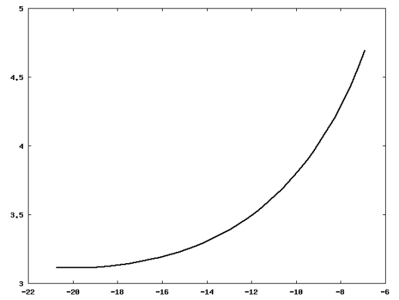
Figure 16: Curve $\left(\ln K,\tfrac{\delta(K)}{(K|\ln K|)^{2.051}}\right)$ where $K$ ranges decreasing from $0.001$ to $10^{-9}$.

The following properties can be obtained easily:

$$(P1) P(\pi,y,\varepsilon) =\frac{y^{2}}{2}-\frac{2}{3}\varepsilon^{2}y^{3}-2,$$

$$(P2) \cos x =1-\frac{y^{2}}{2}+\frac{2}{3}\varepsilon^{2}y^{3},$$

$$(P3) \sin^{2}x =\left(\frac{2}{3}\varepsilon^{2}y-\frac{1}{2}\right)P\left(\pi,y,\varepsilon\right)y^{2}$$

$$=-\frac{2}{3}\varepsilon^{2}\biggl{(}\frac{2}{3}\varepsilon^{2}y-\frac{1}{2}\biggr{)}\biggl{(}y-y_{0}(\varepsilon)\biggr{)}\biggl{(}y-y_{1}(\varepsilon)\biggr{)}\biggl{(}y-y_{2}(\varepsilon)\biggr{)}y^{2},$$

$$(P4) y(-\mathrm{i}s) =Y(s)$$

$$(P5) \sinh\>\!X(s) =-\mathrm{i}\sin x(-\mathrm{i}s)$$

with,

$$y_{0}(\varepsilon)=\dfrac{\sqrt{3}}{\cos\left(\dfrac{\pi-\arccos(4\sqrt{3}\varepsilon^{2})}{3}\right)},\qquad y_{1}(\varepsilon)=\dfrac{\sqrt{3}}{\cos\left(\dfrac{\pi+\arccos(4\sqrt{3}\varepsilon^{2})}{3}\right)},$$

$$y_{2}(\varepsilon)=-\dfrac{\sqrt{3}}{\cos\left(\dfrac{\arccos(4\sqrt{3}\varepsilon^{2})}{3}\right)}.$$

So, we obtain

$$\frac{\df Y}{\df s}(s)=\sinh\>\!X(s)=-\sqrt{-\bigl{(}\nicefrac{{1}}{{2}}-\nicefrac{{2\varepsilon^{2}Y(s)}}{{3}}\bigr{)}\bigl{(}\scalebox{0.85}{$Y(s)-y_{0}(\varepsilon)$}\bigr{)}\bigl{(}\nicefrac{{2\varepsilon^{2}Y(s)}}{{3}}-\nicefrac{{2\varepsilon^{2}y_{1}(\varepsilon)}}{{3}}\bigr{)}\bigl{(}\scalebox{0.75}{$Y(s)-y_{2}(\varepsilon)$}\bigr{)}\scalebox{0.85}{$Y^{2}(s)$}},$$

that is

$$-s^{\ast}={{\int}}_{{}_{y_{0}(\varepsilon)}}^{\scriptscriptstyle\infty}\dfrac{\df Y}{\sqrt{-\bigl{(}\nicefrac{{1}}{{2}}-\nicefrac{{2\varepsilon^{2}Y}}{{3}}\bigr{)}\bigl{(}\scalebox{0.85}{$Y-y_{0}(\varepsilon)$}\bigr{)}\bigl{(}\nicefrac{{2\varepsilon^{2}Y}}{{3}}-\nicefrac{{2\varepsilon^{2}y_{1}(\varepsilon)}}{{3}}\bigr{)}\bigl{(}\scalebox{0.75}{$Y-y_{2}(\varepsilon)$}\bigr{)}\scalebox{0.85}{$Y^{2}$}},}$$

which is a convergent improper integral or, equivalently, through the change of variable $Y=2/v$, we have

$$-s^{\ast}={{\int}}_{{}_{0}}^{\nicefrac{{2}}{{y_{0}(\varepsilon)}}}\!\!\!\!\dfrac{v\df v}{\sqrt{\bigl{(}v-\nicefrac{{8\varepsilon^{2}}}{{3}}\bigr{)}\bigl{(}v-\nicefrac{{2}}{{y_{0}(\varepsilon)}}\bigr{)}\bigl{(}v-\nicefrac{{2}}{{y_{1}(\varepsilon)}}\bigr{)}\bigl{(}v-\nicefrac{{2}}{{y_{2}(\varepsilon)}}\bigr{)}}}.$$

For each given value of $\varepsilon>0$, we have computed, independently, both improper integrals to double check that both values of $s^{*}$ coincide. From the numerical computations done, we conclude that $s^{*}$ has real and imaginary parts, that is, $-s^{*}=-(\operatorname{Re}s^{*}+\mathrm{i}\operatorname{Im}s^{*})=\nicefrac{{\pi}}{{2}}+\delta(\varepsilon)$, where $\operatorname{Re}(-s^{*})=\nicefrac{{\pi}}{{2}}+\delta(\varepsilon)$ and $\operatorname{Im}\delta(\varepsilon)=O(\varepsilon^{2})$.

Our next purpose is to have a fit estimate of $\operatorname{Re}(-s^{*})=\nicefrac{{\pi}}{{2}}+\delta(\varepsilon)$ when varying $\varepsilon$, or, more precisely, of $\delta(\varepsilon)=|\operatorname{Re}(s^{*})|-\nicefrac{{\pi}}{{2}}$. The following fit is obtained

$$\delta(K)=A(K|\ln K|)^{2.051}$$

as can be seen in Figure 16, where the points $\left(\ln K,\tfrac{\delta(K)}{(K|\ln K|)^{2.051}}\right)$ are plotted and we see the tendency towards a constant $A$. So we can infer, taking into account the relation $K=3\varepsilon^{4}$, that $\delta(\varepsilon)$ is of order $\varepsilon^{8}\ln^{2}\varepsilon$.

References

- [1] I. Baldomá. The inner equation for one and a half degrees of freedom rapidly forced Hamiltonian systems. Nonlinearity, 19(6):1415–1445, 2006.
- [2] I. Baldomá, M. Giralt, and M. Guardia. Breakdown of homoclinic orbits to in the RPC3BP (I). Complex singularities and the inner equation. Adv. Math., 408(6), 2022.
- [3] I. Baldomá, M. Giralt, and M. Guardia. Breakdown of homoclinic orbits to in the RPC3BP (II). An asymptotic formula. Adv. Math., 430(109218), 2023.
- [4] I. Baldomá and P. Martín. The inner equation for generalized standard maps. SIAM J. Appl. Dyn. Syst., 11(3):1062–1097, 2012.
- [5] Inmaculada Baldomá, Ernest Fontich, Marcel Guardia, and Tere M. Seara. Exponentially small splitting of separatrices beyond Melnikov analysis: rigorous results. J. Diff. Eqs., 253(12):3304–3439, 2012.
- [6] E. Barrabés, M. Ollé, F. Borondo, D. Farrelly, and J.M. Mondelo. Phase space structure of the hydrogen atom in a circularly polarized microwave field. Phys. D, 241(4):333–349, 2012.
- [7] E. Barrabés, M. Ollé, and Ó. Rodríguez. On the collision dynamics in a molecular model. Phys. D, 460:1–31, 2024.
- [8] Jarosław H. Bauer, Francisca Mota-Furtado, Patrick F. O’Mahony, Bernard Piraux, and Krzysztof Warda. Ionization and excitation of the excited hydrogen atom in strong circularly polarized laser fields. Phys. Rev. A, 90:063402, December 2014.
- [9] I. Bialynicki-Birula, M. Kalinski, and J.H. Eberly. Lagrange equilibrium points in celestial mechanics and nonspreading wave packets for strongly driven Rydberg electrons. Phys. Rev. Lett., 73(13):1777–1780, 1994.
- [10] A.F. Brunello, T. Uzer, and D. Farrelly. Hydrogen atom in circularly polarized microwaves: Chaotic ionization via core scattering. Phys. Rev. A, 55(5):3730–3745, 1997.
- [11] A. Buchleitner, D. Dominique, and J.-C. Gay. Microwave ionization of three-dimensional hydrogen atoms in a realistic numerical experiment. Journal of the Optical Society of America. B, Optical Physics, 12(4):505–519, 1995.
- [12] X. Cabré, E. Fontich, and R. de la Llave. The parameterization method for invariant manifolds I: Manifolds associated to non-resonant subspaces. Indiana University Mathematics Journal, 52, 2003.
- [13] X. Cabré, E. Fontich, and R. de la Llave. The parameterization method for invariant manifolds II: regularity with respect to parameters. Indiana University Mathematics Journal, 52, 2003.
- [14] X. Cabré, E. Fontich, and R. de la Llave. The parameterization method for invariant manifolds III: overview and applications. J. Diff. Eqs., 218, 2005.
- [15] A. Delshams and P. Gutiérrez. Splitting potential and the Poincaré-Melnikov method for whiskered tori in Hamiltonian systems. J. Nonlinear Sci., 10(4):433–476, 2000.
- [16] David Farrelly and T. Uzer. Ionization mechanism of Rydberg atoms in a circularly polarized microwave field. Phys. Rev. Lett., 74:1720–1723, March 1995.
- [17] Laurent Fousse, Guillaume Hanrot, Vincent Lefèvre, Patrick Pélissier, and Paul Zimmermann. Mpfr: A multiple-precision binary floating-point library with correct rounding. ACM Trans. Math. Softw., 33(2):13–es, June 2007.
- [18] Panmimg Fu, T. J. Scholz, J. M. Hettema, and T. F. Gallagher. Ionization of rydberg atoms by a circularly polarized microwave field. Phys. Rev. Lett., 64:511–514, January 1990.
- [19] K. Ganesan and R. GiBarowski. Chaos in the hydrogen atom interacting with external fields. Pramana J. of Physics, 48(2):379–410, 1997.
- [20] Robert Ge¸barowski and Jakub Zakrzewski. Ionization of hydrogen atoms by circularly polarized microwaves. Phys. Rev. A, 51:1508–1519, February 1995.
- [21] Vassili Gelfreich and Carles Simó. High-precision computations of divergent asymptotic series and homoclinic phenomena. Discr. Contin. Dyn. Syst. Ser. B, 10(2-3):511–536, 2008.
- [22] Andreas Griewank and Andrea Walther. Evaluating Derivatives. Society for Industrial and Applied Mathematics, second edition, 2008.
- [23] Jennifer A. Griffiths and David Farrelly. Ionization of rydberg atoms by circularly and elliptically polarized microwave fields. Phys. Rev. A, 45:R2678–R2681, Mar 1992.
- [24] Marcel Guardia. Splitting of separatrices in the resonances of nearly integrable Hamiltonian systems of one and a half degrees of freedom. Discr. Contin. Dyn. Syst., 33(7):2829–2859, 2013.
- [25] Marcel Guardia, Carme Olivé, and Tere M. Seara. Exponentially small splitting for the pendulum: a classical problem revisited. J. Nonlinear Sci., 20(5):595–685, 2010.
- [26] J. Guckenheimer and P. Holmes. Nonlinear oscillations, dynamical systems and bifurcations of vector fields. Springer-Verlag, 1983.
- [27] À. Haro, M. Canadell, JL. Figueras, A. Luque, and J.M. Mondelo. The Parameterization Method for Invariant Manifolds: From Rigorous Results to Effective Computations. Applied Mathematical Sciences 195. Springer International Publishing, 1 edition, 2016.
- [28] Charles Jaffé, D. Farrelly, and T. Uzer. Transition state theory without time-reversal symmetry: Chaotic ionization of the hydrogen atom. Phys. Rev. Lett., 84:610–613, Jan 2000.
- [29] À. Jorba and M. Zou. A software package for the numerical integration of ODEs by means of high-order Taylor methods. Experiment. Math., 14(1):99–117, 2005.
- [30] Oksana Koltsova, Lev Lerman, Amadeu Delshams, and Pere Gutiérrez. Homoclinic orbits to invariant tori near a homoclinic orbit to center-center-saddle equilibrium. Phys. D, 201(3-4):268–290, 2005.
- [31] Mercè Ollé. To and fro motion for the hydrogen atom in a circularly polarized microwave field. Comm. Nonlinear Sci. Numer. Simulat., 54:286–301, 2018.
- [32] Mercè Ollé and Juan Ramón Pacha. Hopf bifurcation for the hydrogen atom in a circularly polarized microwave field. Comm. Nonlinear Sci. Numer. Simulat., 62:27–60, 2018.
- [33] M. J. Raković and Shih-I Chu. Approximate dynamical symmetry of hydrogen atoms in circularly polarized microwave fields. Phys. Rev. A, 50:5077–5080, December 1994.
- [34] Kazimierz Rzaewski and Bernard Piraux. Circular Rydberg orbits in circularly polarized microwave radiation. Phys. Rev. A, 47:R1612–R1615, March 1993.
- [35] Carles Simó. Averaging under fast quasiperiodic forcing. In Hamiltonian mechanics (Toruń, 1993), volume 331 of NATO Adv. Sci. Inst. Ser. B: Phys., pages 13–34. Plenum, New York, 1994.
- [36] Satya Undurti, Han Xu, Xiaoshan Wang, Atia Noor, William Wallace, Nicolas Douguet, Alexander Bray, I. Ivanov, Klaus Bartschat, A. Kheifets, Robert Sang, and Igor Litvinyuk. Attosecond angular streaking and tunnelling time in atomic hydrogen. Nature, 568:75–77, 04 2019.
- [37] J. Zakrzewski, D. Delande, J.-C. Gay, and K. Rzazewski. Ionization of highly excited hydrogen atoms by a circularly polarized microwave field. Phys. Rev. A, Atomic, Molecular, and Optical Physics, 47(4A):R2468–R2471, 1993.