Performance Analysis of uRLLC in scalable Cell-free RAN System

Abstract

As an essential part of mobile communication systems that beyond the fifth generation (B5G) and sixth generation (6G), ultra reliable low latency communication (uRLLC) places strict requirements on latency and reliability. In recent years, with the improvement of mobile communication network performance, centralized and distributed processing of cell-free mMIMO has been widely studied, and wireless access networks (RAN) have also become a widely studied topic in academia. This paper analyzes the performance of a novel scalable cell-free RAN (CF-RAN) architecture with multiple edge distributed units (EDUs) in the scenario of finite block length. The upper and lower bounds on its spectral efficiency (SE) performance are derived, and the complete set’s formula and distributed processing can be used as their two exceptional cases, respectively. Secondly, the paper further considers the distribution of users and large-scale fading models and studies the position distribution of remote radio units (RRUs). It is found that a uniform distribution of RRUs is beneficial for improving the SE of finite block length under specific error rate performance, and RRUs need to be interwoven as much as possible under multiple EDUs. This is different from traditional multi-node clustering centralized collaborative processing. The paper compares the performance of Monte Carlo simulation and multi-RRU clustering group collaborative processing. At the same time, this article verifies the accuracy of the space-time exchange theory in the CF-RAN scenario. Through scalable EDU deployment, a trade-off between latency and reliability can be achieved in practical systems and exchanged with spatial degrees of freedom. This implementation can be seen as a distributed and scalable implementation of the space-time exchange theory.

I INTRODUCTION

With the continuous development of communication technology and the increasing demand for data transmission, the fifth-generation mobile communication system (5G) has been widely promoted. The main characteristics of 5G are higher data transmission speed, lower transmission latency, higher reliability, and a significantly higher number of connections compared to the fourth generation systems (4G). Specifically, 5G regards low latency and high-reliability communication (uRLLC) as one of the three essential application scenarios [1].

URLLC must meet the requirements for transmission reliability and low latency. The work around uRLLC is mainly based on the research in citepolyanskiy2010channel for the scenario of finite blocklength. The channel capacity analyzed in traditional communication systems is based on infinite block length. In finite block length, the traditional Shannon capacity based on the law of large numbers is no longer applicable [2]. 5G has adopted various technologies to achieve low latency and high reliability, among which is Multi TRP, one of the most important. In the long-term evolution of the fourth-generation mobile communication system (4G-LTE), multi-point transmission (CoMP) is also used for multi-point transmission and reception. Multi TRP and CoMP are critical technologies for improving spectrum efficiency, peak rate, and reliability, which can collaboratively process signals between multiple base stations, thereby improving network performance. Although CoMP was proposed in 4G LTE, it was not until the R16 version of 5G-NR that a standardized implementation of incoherent multi-TRP was provided and widely used in commercial systems [3, 4]. Now, the standard is being developed for Multi TRP Coherent Joint Transmission (CJT), which will further improve the network’s performance [5]. Currently, academia and industry have begun to research the sixth-generation mobile communication system (6G) technology to meet higher communication needs in the future [6]. Compared to 5G, 6G requires higher reliability and lower transmission latency [7, 8], which requires more advanced technology. In recent research work, [9] pointed out several critical limitations of uRLLC in the current 5G system and pointed out that scalability will be one of the key technical indicators for eXtreme ultra-reliable and low-latency communication (xURLLC) in 6G. [10] provided a comprehensive review of existing 5G uRLLC technology, shedding light on their associated risks and challenges in the context of future 6G communication systems and pointed out that understanding the core principles and navigating the tradeoffs in vital quality of service requirements of 6G xURLLC remains a complex challenge. Various types of interference challenges in uRLLC were discussed in [11] and classified according to their deployment, design, technology, usage, and propagation characteristics, and extreme throughput performance under very low latency and up to $10^{-9}$ percentile success probability applications were evaluated. [12] provided a comprehensive review and comparison of different candidate decoding techniques for uRLLC regarding their error-rate performance and computational complexity for structured and random short codes.

The concept of spatiotemporal exchangeability was novelly proposed in [13], and a specific implementation scheme was proposed in [14]. In the $15dB$ signal-to-noise ratio (SNR) scenario, the capacity collapse effect caused by finite block length can be compensated by increasing the number of streams in the system with the deployment in the spatial domain. By appropriately selecting the code rate, block length, and the number of codewords in the time and spatial domains, the coding scheme proposed in [14] can achieve a good tradeoff between transmission delay and reliability. In subsequent work, [15] proved the exchangeability theory, deriving a closed expression for channel dispersion in massive MIMO scenarios.

Compact and explicit performance bounds of finite blocklength coded MIMO were formed to explore the relationship between blocklength, decoding error probability, rate, and DoF in different coding modes [16]. The above point-to-point work thoroughly and rigorously verified the idea of increasing the spatial degrees of freedom (DoF) to compensate for the shortcomings of finite block length. Compact and explicit performance bounds of finite blocklength coded MIMO were formed to explore the relationship between blocklength, decoding error probability, rate and DoF in different coding modes in

In 6G, cell-free massive multi-input multi-output technology (CF-mMIMO) will be an important research direction. CF-mMIMO is a more revolutionary technology that can break the traditional cellular architecture and achieve cell-free communication with more flexible and efficient network coverage. There have been many studies on cell-free systems in 5G [17, 18], but the research in 6G will be more in-depth and extensive. [2] pointed out that multi-antenna MIMO is a more general extension of classical Shannon information theory. Suppose channel state information (CSI) is globally known. In that case, channel models and capacity analysis in complex application scenarios such as single-user, multi-user, or multi-base station joint processing can be described in a unified form. The spatial freedom of MIMO channels can be artificially increased by increasing the antenna configuration at the transmitting and receiving ends. Under specific theoretical assumptions, future mobile communication systems have no so-called performance limit [19].

Researching how to utilize cell-free architecture to implement uRLLC in 6G systems is worthwhile. [20] pointed out that cell-free architecture with a large number of distributed antennas has macro-diversity and spatial sparsity characteristics, which can further improve the performance of uRLLC. [21] and [22] derived a rate closed-form lower bound with imperfect CSI based on different precoding and combining schemes. By jointly optimizing pilot power and payload power, the global optimal pilot power was derived, and using successive convex approximation (SCA), the non-convex problem was transformed into a series of sub-problems for processing. By deploying more access points (APs), the quality of uRLLC services will benefit. [23] investigated the potential of CFmMIMO to multiplex uRLLC and other services by exploiting the sole spatial diversity through network slicing and adopting greedy pilot allocation to minimize pilot contamination. A particular type of conjugate beamforming (CB) was proposed in [24] that only required local CSI, and a new path-following algorithm was developed to optimize uRLLC rates and CFmMIMO energy efficiency. [25] proposed a general framework to characterize the achievable grouping error probability in the CF-mMIMO. Based on saddlepoint approximation and scaling-based random coding union (RCUs), the performance of CF-mMIMO supporting finite block length under the high-reliability target required by uRLLC is analyzed. [26] investigated the resource allocation problem of CF-mMIMO assisted uRLLC systems, derived a closed form rate lower bound with imperfect CSI and pilot contamination, proposed a new pilot allocation scheme that balances the ratio of pilot length to payload, and jointly optimized pilot and payload power, balancing estimated channel gain and pilot contamination. In the deployment of CF-mMIMO supporting uRLLC, some challenges still need to be solved. Firstly, CF-mMIMO requires more antennas to achieve lower transmission latency and higher reliability. For multi-user scenario processing, traditional centralized processing complexity will be very high. The cell-free deployment must face the problem of scalability. Secondly, more efficient architecture deployment and advanced correlation algorithms are needed to support the complexity of distributed cell-free systems. Therefore, the research on CF-mMIMO is still in the theoretical stage.

Currently, a lot of work is focused on the scalability of CFmMIMO correlation and the distribution of AP positions. [27] introduced the classification method of CF-mMIMO with four different implementation levels, from fully centralized to fully distributed, and analyzed the spectral efficiency (SE) performance of spatially correlated fading and different combining schemes. Starting from the scalability of CF-mMIMO, [28] investigated the cell-free radio access network (CF-RAN) under the O-RAN architecture and investigated the uplink and downlink SE of CF-mMIMO and user association based on artificial intelligence. [29] considered the CF-MIMO, where the AP position satisfies the Poisson point process (PPP) and derives the downlink coverage probability and achievable rate. [30] assumed that the distribution of APs is random based on PPP, simulating the actual behavior of APs on mobile networks. Considering the maximum ratio combining (MRC) and minimum mean square error (MMSE) combining at the AP receiver to estimate channel statistics, they derived the uplink SE of CF-MIMO and proved the relationship between AP density/distribution and system SE. The approximate achievable rates of several linear pre-encoders and detectors were considered in the uplink and downlink of non-cooperative multi-cellular time division systems. [31] investigated the performance of channel hardening and confidence propagation in real-world random AP deployment in CF-mMIMO systems. [32] derived two approximate values for the reachable uplink rate with perfect/imperfect CSI in CF-mMIMO, and all these approximate values converge to the classical boundaries implemented in traditional massive MIMO systems where the BS antenna is located at the same position. [33] compared the asymptotic rate performance of downlink multi-user systems with multiple BS antennas, which are either located in the same location or uniformly distributed within the cell. Two representative linear precoding schemes, Maximum Ratio Transmission (MRT) and zero-forcing (ZF) beamforming, were considered to characterize the impact of BS antenna layout on rate performance. [34] derived the lower capacity limits for MRC, ZF, and MMSE detection in a centralized processing scenario. [35] proposed a scalable architecture for CF-mMIMO systems through distributed transceivers and scalable collaborative transmission, which can further improve the network’s performance. Based on this, potential vital technologies such as channel information acquisition, transceiver design, dynamic user and access point association, and new duplex were introduced, and the performance of distributed receiver design was evaluated.

However, we have noticed several shortcomings in the current research: (1) Existing work on the cell-free implementation of uRLLC mostly failed to consider the scalability and implementability of the system; (2) Considering the actual deployment of cell-free APs, many studies analyzed the SE based on stochastic geometry architecture; The precoding and combining schemes have not fully utilized the collaborative characteristics of cell-free, and there is little research on collaborative transceivers based on interference suppression; (3) The research on scalable cell-free was nearly all based on infinite blocklength, without considering the impact of finite blocklength on system performance, which cannot meet the uRLLC requirement.

Therefore, in response to the above issues, relying on the currently validated spatiotemporal exchangeability theory [15] in point-to-point transmission, this paper will implement uRLLC for scalable cell-free systems. The main contributions of this paper are as follows:

• Analyzing the SE of a new scalable cell-free RAN with multiple edge distributed units (EDUs) under finite block length.

• A modified graph coloring algorithm for interleaving correlation is used to analyze the correlation performance of remote radio units (RRUs) under multiple EDUs that can improve the system SE under latency and reliability constraints.

• By deploying scalable EDUs, a compromise between reliability and latency is exchanged with spatial DoF, further expanding and verifying the accuracy of the distributed space-time exchangeability theory.

Organization:

Notation: bold uppercase $\mathbf{A}$ (bold lowercase $\mathbf{a}$) denotes a matrix (a vector). ${{\mathbf{I}}_{N}}$ and ${{\mathbf{0}}_{M,N}}$ denote the $N\times N$ dimensional identity matrix and the $M\times N$ dimensional all-zero matrix, respectively. ${\left(\cdot\right)^{H}}$, ${\left(\cdot\right)^{T}}$ , ${\left(\cdot\right)^{*}}$, ${\left(\cdot\right)^{-1}}$ and ${\left(\cdot\right)^{\dagger}}$ stand for the conjugate transpose, transpose, conjugate, inverse and pseudo-inverse, respectively. ${\mathrm{diag}}\left\{{\mathbf{a}}\right\}$, ${\mathrm{diag}}\left\{{\mathbf{A}}\right\}$ and ${\mathrm{blkdiag}}\left\{{\mathbf{A}_{1}},\cdots,{\mathbf{A}_{N}}\right\}$ represent a diagonal matrix with $\mathbf{a}$ along its main diagonal, a vector constructed by the main diagonal of the matrix $\mathbf{A}$, a block diagonal matrix , respectively. $\otimes$ denotes the Kronecker product of two matrices. $\ell_{0}$ , $\ell_{1}$ and $\ell_{2}$ norm of vectors are denoted by $\left\|\cdot\right\|_{0}$, $\left\|\cdot\right\|_{1}$ and $\left\|\cdot\right\|_{2}$, respectively. ${\mathcal{CN}}\left(\bm{\mu},\mathbf{R}\right)$ denotes the complex Gaussian distribution with mean $\bm{\mu}$ and covariance matrix $\mathbf{R}$. ${\mathbb{E}}\left\{\cdot\right\}$ is the expectation operator. Finally, $\backslash$ denotes the set subtraction operation.

II SYSTEM MODEL

In this section, we introduce the implementation of the CF-mMIMO system. Under the new architecture, we analyze the uplink SE of CF-mMIMO, and the combining strategy adopts a unified representation. We consider a CF-mMIMO with $L$ $N$ antenna RRUs and $K$ single-antenna user equipments (UEs). Assuming $LN$ is large, and $L\gg K$. At the $l$-th RRU, the received signal ${{\bf{y}}_{{\rm{UL}},l}}$ can be expressed as [27]:

$${{\bf{y}}_{{\rm{UL}},l}}=\sum\limits_{k=1}^{K}{{{\bf{h}}_{l,k}}\sqrt{{p_{k}}}{s_{k}}}+{{\bf{z}}_{l}},$$ (1)

where ${s_{k}}$ denotes the transmitted symbol of the $k$-th UE, ${p_{k}}$ denotes the uplink transmission power of the $k$-th UE, ${{\bf{h}}_{l,k}}$ represents the $N\times 1$ CSI from the $k$-th UE to the $l$-th RRU and ${{\bf{z}}_{l}}\sim{{\cal CN}}\left({0,{\sigma_{\rm UL}^{2}}{{\bf{{I}}}_{N}}}\right)$ represents the additive white gaussian noise (AWGN).

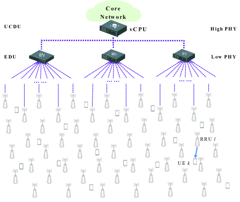
Figure 1: The system model has $M$ EDUs, $L$ RRUs, each RRU with $N$ antennas, and $K$ single-antenna UEs.

We assume there are $M$ EDUs in the system, as shown in Fig. 1. Let the channel vector from the $k$-th UE to all RRUs be:

$${{\mathbf{h}}_{k}}={{\left[\mathbf{h}_{k,1}^{\rm T},\mathbf{h}_{k,2}^{\rm T}\cdots\mathbf{h}_{k,L}^{\rm T}\right]}^{\rm T}}\in{{\mathbb{C}}^{LN}},$$ (2)

among them, ${{\mathbf{h}}_{k}}={{{\mathbf{B}}^{1/2}_{k}}}{{\mathbf{g}}_{k}}$, the large-scale fading matrix is ${{\mathbf{B}}_{k}}={\rm diag}\left({{\beta}_{k,1}},{{\beta}_{k,2}},\cdots,{{\beta}_{k,L}}\right)\otimes{{\mathbf{I}}_{N}}$. The correlated Rayleigh fading channel vector ${{\mathbf{g}}_{k}}$ is distributed as: ${{\mathbf{g}}_{k}}\sim{{\mathcal{CN}}}\left(\mathbf{0},{{\mathbf{R}}_{k}}\right)$, where ${{\mathbf{R}}_{k}}=\operatorname{diag}\left({{\mathbf{R}}_{k,1}},\ldots,{{\mathbf{R}}_{k,L}}\right)\in{{\mathbb{C}}^{LN\times LN}}$ represents the block diagonal spatial correlation matrix of user $k$.

According to [28], the uplink signal-to-interference plus noise ratios (SINRs) for the $k$-th user is:

$$\gamma_{k}^{({\rm{UL}},{\rm{d}})}=\frac{{{p_{k}}{{\left|{\sum\limits_{m=1}^{M}\mathbb{E}{\left({{\bf{v}}_{k,m}^{\rm{H}}{{\bf{D}}_{k,m}}{{\bf{h}}_{k,m}}}\right)}}\right|}^{2}}}}{{\sum\limits_{i=1,i\neq k}^{K}{{p_{i}}}\mathbb{E}{{\left|{\sum\limits_{m=1}^{M}{{\bf{v}}_{k,m}^{\rm{H}}{{\bf{D}}_{k,m}}{{\bf{h}}_{i,m}}}}\right|}^{2}}+\sigma_{{\rm{UL}}}^{2}\mathbb{E}\left({\sum\limits_{m=1}^{M}{{{\left\|{{{\bf{D}}_{k,m}}{{\bf{v}}_{k,m}}}\right\|}^{2}}}}\right)}},$$ (3)

where ${\bf{v}}_{k,m}$ is combining vector of user $k$. ${{\bf{D}}_{k,m}}$ is the association matrix between the user and the RRU, ${{\mathbf{D}}_{k}}={\rm diag}\left({{\delta}_{k,1}},{{\delta}_{k,2}},\cdots,{{\delta}_{k,L}}\right)\otimes{{\mathbf{I}}_{N}}$, where ${{\delta}_{k,l}}=1$ if RRU $l$ is associated with user $k$, otherwise ${{\delta}_{k,l}}=0$.

For analysis, we assume perfect CSI, with full association between users and RRUs. Considering a single-antenna RRU scenario, i.e., $N=1$, ${{\bf{D}}_{k,m}}={{\bf{I}}_{k,m}}$. Taking uplink reception as an example, the uplink reception SINR can be expressed in a general way as

$$\gamma_{k}^{({\rm{UL}},{\rm{d}})}=\frac{{{p_{k}}{{\left|{\sum\limits_{m=1}^{M}{{\bf{v}}_{k,m}^{\rm{H}}{{\bf{h}}_{k,m}}}}\right|}^{2}}}}{{\sum\limits_{i=1,i\neq k}^{K}{{p_{i}}}{{\left|{\sum\limits_{m=1}^{M}{{\bf{v}}_{k,m}^{\rm{H}}{{\bf{h}}_{i,m}}}}\right|}^{2}}+\sigma_{{\rm{UL}}}^{2}\left({\sum\limits_{m=1}^{M}{\left\|{{\bf{v}}_{k,m}}\right\|{{}^{2}}}}\right)}}.$$ (4)

Clearly, centralized and fully distributed configurations can be introduced as exceptional cases for $M=1$ and $M=L$, respectively [36]. In the next section, we take uplink analysis as an example and analyze the performance relationship between uplink SE and RRU location distribution.

Considering the impact of the finite blocklength (FBL) scenario, under AWGN channel conditions, given the required transmission error probability of the system ${{\varepsilon}}$ and the blocklength of the system transmission $n$, it is known from [37] that using non-Gaussian codebooks can achieve the maximum channel rate. Under finite blocklength, the SE of the $k$-th user can be closely approximated as

$${{R}_{k}}\approx{{\log}_{2}}\left(1+{{\gamma}_{k}}\right)-\sqrt{\frac{{{V}_{k}}}{n}}{{Q}^{-1}}\left({{\varepsilon}_{k}}\right),$$ (5)

where the channel dispersion term is

$${{V}_{k}}\text{=}\left(1-{{\left(1+{{\gamma}_{k}}\right)}^{-2}}\right){{\log}_{2}}^{2}e,$$ (6)

in which ${{Q}^{-1}}$is the inverse of $Q(x)=\frac{1}{\sqrt{2\pi}}\int_{x}^{\infty}{{{e}^{-\frac{{{t}^{2}}}{2}}}}\text{d}t$.

Considering the independence of the equivalent cell-free channel, similar to the treatment in [38], the system SE can be expressed as

$$R =C-\sqrt{\frac{V}{n}}{Q^{-1}}\left(\varepsilon\right)$$ (7)

$$=\sum\limits_{i=1}^{K}{{{\log}_{2}}\left(1+{{\gamma}_{i}}\right)}-\sqrt{\frac{K-\sum\limits_{i=1}^{K}{\frac{1}{{{\left(1+{{\gamma}_{i}}\right)}^{2}}}}}{n}}{{Q}^{-1}}\left({{\varepsilon}}\right),$$

where $C$ is the traditional channel capacity and $V$ is the total channel dispersion parameter under multiple UEs.

Remark 1: Considering the multi-user interference, the SE analysis of UEs under finite block length becomes very complex. By adopting cooperative combining schemes with interference suppression, interference can be effectively mitigated, especially when the channel estimation is perfect, thus approximating the channel condition as an AWGN channel. This approach is adopted in many current research works [39, 40]. The following section will analyze the system’s SE with the ZF combining scheme for theoretical rigor.

III SE Analysis with Finite Blocklength

III-A Upper and Lower Bounds of SE

For the ZF combining of perfect CSI [41], the original centralized combining matrix is ${\bf{V}}={\bf{H}}{\left({{{\bf{H}}^{\bf{H}}}{\bf{H}}}\right)^{-1}}\in{\mathbb{C}^{K\times LN}}$, where it is assumed that the RRU is single-antenna. Therefore, ${\bf{H}}\buildrel\Delta\over{=}[{{\bf{h}}_{1}},\ldots,{{\bf{h}}_{k}},\ldots,{{\bf{h}}_{K}}]\in{\mathbb{C}^{L\times K}}$. Since ZF completely nullifies interference, the interference received by each EDU is $0$. As the number of EDUs increases, the matrix dimensions continually decrease; we have:

$$\gamma_{k}^{({\rm{UL}},{\rm{d}})} =\frac{{{p_{k}}{{\left|{\sum\limits_{m=1}^{M}{{\bf{v}}_{k,m}^{\rm{H}}{{\bf{h}}_{k,m}}}}\right|}^{2}}}}{{\sum\limits_{i=1,i\neq k}^{K}{{p_{i}}}{{\left|{\sum\limits_{m=1}^{M}{{\bf{v}}_{k,m}^{\rm{H}}{{\bf{h}}_{i,m}}}}\right|}^{2}}+\sigma_{{\rm{UL}}}^{2}\left({\sum\limits_{m=1}^{M}{{{\left\|{{{\bf{v}}_{k,m}}}\right\|}^{2}}}}\right)}}\;$$ (8)

$$=\frac{{{p_{k}}{M^{2}}}}{{\sum\limits_{m=1}^{M}{{{\left\|{{{\bf{v}}_{k,m}}}\right\|}^{2}}}}},$$

where

$${{\bf{V}}_{m}}={{\bf{H}}_{m}}{\left({{\bf{H}}_{m}^{\bf{H}}{{\bf{H}}_{m}}}\right)^{-1}},$$ (9)

${{\bf{v}}_{k,m}}$ is the $k$-th column of ${{\bf{V}}_{m}}$. Here, the condition for precoding requires that the number of antennas in the EDU ${L_{m}}$ is much greater than the number of UE $K$, and the UE set is ${\cal K}$. Under perfect CSI, the SINR does not include interference information.

Therefore, the total average SE of the system is:

$$R=\sum\limits_{i=1}^{K}{{{\log}_{2}}\left(1+\frac{{{p}_{k}}{{M}^{2}}}{\sum\limits_{m=1}^{M}{{{\left\|{{\mathbf{v}}_{k,m}}\right\|}^{2}}}}\right)}-\frac{{{Q}^{-1}}\left(\varepsilon\right)}{\sqrt{n}}\sqrt{K-\sum\limits_{i=1}^{K}{\frac{1}{{{\left(1+{{{p}_{k}}{{M}^{2}}}/{\sum\limits_{m=1}^{M}{{{\left\|{{\mathbf{v}}_{k,m}}\right\|}^{2}}}}\;\right)}^{2}}}}},$$ (10)

From (9), we have that

$${{\left\|{{\mathbf{v}}_{k,m}}\right\|}^{2}}=\left[{{{\left({{\bf{H}}_{m}^{\rm{H}}{{\bf{H}}_{m}}}\right)}^{-1}}}\right]_{kk}$$ (11)

Among them, different channel matrices ${{\bf{H}}_{1}},{{\bf{H}}_{2}},\ldots,{{\bf{H}}_{M}}$ are independent, where ${{\bf{H}}_{m}}\in{\mathbb{C}^{{L_{m}}\times K}}$. The number of RRUs in an EDU satisfies the following three expressions,

$$\;\;\;{L_{1}}+{L_{2}}+\cdots+{L_{M}}=L,$$ (12a)

$$\;\;\;{{\cal L}_{1}}\cup{{\cal L}_{2}}\cup\cdots\cup{{\cal L}_{M}}={\cal L},$$ (12b)

$$\;\;\;\left({{\cal L}_{1}}\cap{{\cal L}_{2}}\right)\cup\cdots\cup\left({{\cal L}_{1}}\cap{{\cal L}_{M}}\right)\cup\cdots\cup\left({{\cal L}_{M-1}}\cap{{\cal L}_{M}}\right)=\varnothing,$$ (12c)

where ${\cal L}=\{l|\forall l=1,\ldots,L\}$. Clearly, the system’s ergodic achievable sum SE can be expressed in the form of its expectation, i.e., $\overline{R}={\mathbb{E}_{{{\bf{H}}_{1}},{{\bf{H}}_{2}},\ldots,{{\bf{H}}_{M}}}}\left\{{\sum\limits_{i=1}^{K}{{R_{i}}}}\right\}$. We denote the LHS of the ergodic achievable SE in (10) as $X={\mathbb{E}_{{{\bf{H}}_{1}},{{\bf{H}}_{2}},\ldots,{{\bf{H}}_{M}}}}\left\{{\sum\limits_{i=1}^{K}{{{\log}_{2}}\left({1+\frac{{{p_{k}}{M^{2}}}}{{\sum\limits_{m=1}^{M}{{{\left\|{{{\bf{v}}_{k,m}}}\right\|}^{2}}}}}}\right)}}\right\}$, and the RHS of (10) as $Y=\frac{{{Q}^{-1}}\left({{\varepsilon}}\right)}{\sqrt{n}}{{\mathbb{E}}_{{{\mathbf{H}}_{1}},{{\mathbf{H}}_{2}},\ldots,{{\mathbf{H}}_{M}}}}\left\{\sqrt{{{V}}}\right\}$.

Next, we will analyze the left and right terms separately. For the LHS in (10), using Jensen’s inequality, the upper bound can be expressed as,

$$X\leq\sum\limits_{i=1}^{K}{{{\log}_{2}}\left({1+{\mathbb{E}_{{{\bf{H}}_{1}},{{\bf{H}}_{2}},\ldots,{{\bf{H}}_{M}}}}\left\{{\frac{{p_{i}}{M^{2}}}{{\sum\limits_{m=1}^{M}{{\left[{{{\left({{\bf{H}}_{m}^{\rm{H}}{{\bf{H}}_{m}}}\right)}^{-1}}}\right]}_{kk}}}}}\right\}}\right)}.$$ (13)

Similarly, the lower bound of the LHS can be expressed as,

$$X\geq\sum\limits_{i=1}^{K}{{{\log}_{2}}\left({1+\frac{{{p_{i}}{M^{2}}}}{{{\mathbb{E}_{{{\bf{H}}_{1}},{{\bf{H}}_{2}},\ldots,{{\bf{H}}_{M}}}}\left\{{{\sum\limits_{m=1}^{M}{{{\left[{{{\left({{\bf{H}}_{m}^{\rm{H}}{{\bf{H}}_{m}}}\right)}^{-1}}}\right]}_{kk}}}}}\right\}}}}\right)}.$$ (14)

Remark 2: In comparison with the results obtained from centralized processing presented in [32], expressions (13) and (14) in our study compute the average SINR in the ergodic achievable rate by taking the expectations of the channel matrices for different EDUs independently. This approach utilizes the channel’s independence between the EDUs and the UEs.

Therefore, for the RHS of (10), using Jensen’s inequality, we can have the same treatment, and the upper bound can be expressed as,

$$Y\leq\frac{{{Q}^{-1}}\left({{\varepsilon}}\right)}{\sqrt{n}}\sqrt{K-\sum\limits_{i=1}^{K}{1/{{\left({1+\frac{{{p_{k}}{M^{2}}}}{S}}\right)}^{2}}}}.$$ (15)

where $S={{{\mathbb{E}_{{{\bf{H}}_{1}},{{\bf{H}}_{2}},\ldots,{{\bf{H}}_{M}}}}\left\{{\sum\limits_{m=1}^{M}{{{\left[{{{\left({{\bf{H}}_{m}^{\rm{H}}{{\bf{H}}_{m}}}\right)}^{-1}}}\right]}_{kk}}}}\right\}}}$.

Similarly, the lower bound of can be expressed as,

$$Y\geq\frac{{{Q}^{-1}}\left({{\varepsilon}}\right)}{\sqrt{n}}\sqrt{K-\sum\limits_{i=1}^{K}{1/{{\left({1+{\mathbb{E}_{{{\bf{H}}_{1}},{{\bf{H}}_{2}},\ldots,{{\bf{H}}_{M}}}}\left\{T\right\}}\right)}^{2}}}}.$$ (16)

where $T={\frac{{{p_{k}}{M^{2}}}}{{\sum\limits_{m=1}^{M}{{{\left[{{{\left({{\bf{H}}_{m}^{\rm{H}}{{\bf{H}}_{m}}}\right)}^{-1}}}\right]}_{kk}}}}}}$.

The fraction within the expectation must be analyzed using the matrix inversion formula for the above expressions.

$${\left({{\bf{H}}_{m}^{\rm{H}}{{\bf{H}}_{m}}}\right)^{-1}}=\frac{{{{\left({{\bf{H}}_{m}^{\rm{H}}{{\bf{H}}_{m}}}\right)}^{*}}}}{{\det\left({{\bf{H}}_{m}^{\rm{H}}{{\bf{H}}_{m}}}\right)}}.$$ (17)

Let matrix $\bf{G}_{m}={{\bf{H}}_{m}^{\rm{H}}{{\bf{H}}_{m}}}$, $\bf{G}_{m,k}$ be the algebraic cofactor of the $k,k$-th element of matrix $\bf{G}_{m}$, so the $k,k$-th element of the inverse matrix ${{\bf{H}}_{m}^{\rm{H}}{{\bf{H}}_{m}}}$ is expressed as,

$${{{\left[{{{\left({{\bf{H}}_{m}^{\rm{H}}{{\bf{H}}_{m}}}\right)}^{-1}}}\right]}_{kk}}}=\frac{\det\left({{{\bf{G}}_{m,k}}}\right)}{{\det\left({{{\bf{G}}_{m}}}\right)}}.$$ (18)

Therefore,

$$\frac{1}{{\sum\limits_{m=1}^{M}{{{\left\|{{{\bf{v}}_{k,m}}}\right\|}^{2}}}}}=\frac{1}{{\sum\limits_{m=1}^{M}{{{\left[{{{\left({{\bf{H}}_{m}^{\rm{H}}{{\bf{H}}_{m}}}\right)}^{-1}}}\right]}_{kk}}}}}=\frac{1}{{\sum\limits_{m=1}^{M}{{{\left[\frac{\det\left({{{\bf{G}}_{m,k}}}\right)}{{\det\left({{{\bf{G}}_{m}}}\right)}}\right]}}}}}.$$ (19)

Using Jensen’s inequality, we can obtain:

$$\frac{1}{{\frac{1}{M}\left[{\sum\limits_{i=1}^{M}{\frac{{\det\left({{{\bf{G}}_{i,k}}}\right)}}{{\det\left({{{\bf{G}}_{i}}}\right)}}}}\right]}}\leq\frac{1}{M}\sum\limits_{i=1}^{M}{\frac{1}{{\frac{{\det\left({{{\bf{G}}_{i,k}}}\right)}}{{\det\left({{{\bf{G}}_{i}}}\right)}}}}}=\frac{1}{M}\sum\limits_{i=1}^{M}{\frac{{\det\left({{{\bf{G}}_{i}}}\right)}}{{\det\left({{{\bf{G}}_{i,k}}}\right)}}}.$$ (20)

Therefore, according to (20), the upper bound of the LHS $X$ and the RHS $Y$ in (13) can be written on the top of next page.

$$X\leq{X^{{\rm{ub}}}}=\sum\limits_{i=1}^{K}{{{\log}_{2}}\left({1+{p_{i}}M{\mathbb{E}_{{{\bf{H}}_{1}},{{\bf{H}}_{2}},\ldots,{{\bf{H}}_{M}}}}\left\{{\frac{1}{M}\sum\limits_{m=1}^{M}{\frac{{\det\left({{{\bf{G}}_{m}}}\right)}}{{\det\left({{{\bf{G}}_{m,i}}}\right)}}}}\right\}}\right)}.$$ (21)

$$Y\leq{Y^{{\rm{ub}}}}=\frac{{{Q}^{-1}}\left({{\varepsilon}}\right)}{\sqrt{n}}\sqrt{K-\sum\limits_{i=1}^{K}{1/{{\left({1+{p_{i}}M{\mathbb{E}_{{{\bf{H}}_{1}},{{\bf{H}}_{2}},\ldots,{{\bf{H}}_{M}}}}\left\{{\frac{1}{M}\sum\limits_{m=1}^{M}{\frac{{\det\left({{{\bf{G}}_{m}}}\right)}}{{\det\left({{{\bf{G}}_{m,i}}}\right)}}}}\right\}}\right)}^{2}}\;}}.$$ (22)

Using the Schur complement lemma [33], we have,

$${\frac{{\det\left({{{\bf{G}}_{i}}}\right)}}{{\det\left({{{\bf{G}}_{i,k}}}\right)}}} \mathop{\approx}\limits^{{L_{m}}\gg K}{\left\|{{{\bf{h}}_{k,m}}}\right\|^{2}}-\sum\limits_{j\neq k,j\in{\cal K}}\cdot\frac{{{{\bf{h}}_{k,m}}}{\bf{h}}_{j,m}^{\rm{H}}{{\bf{h}}_{j,m}}{\bf{h}}_{k,m}^{\rm{H}}}{{{{\left\|{{{\bf{h}}_{j,m}}}\right\|}^{2}}}}$$ (23)

$$={\left\|{{{\bf{h}}_{k,m}}}\right\|^{2}}-\sum\limits_{j\neq k,j\in{\cal K}}{{{\left|{{h_{k,l_{j,m}^{*}}}}\right|}^{2}}}=\sum\limits_{l\in{{\widetilde{\cal L}}_{m,k}}}{{{\left|{{h_{k,l}}}\right|}^{2}}},$$

where ${\widetilde{\cal L}_{m,k}}={{\cal L}_{m}}-{\left\{{l_{j,m}^{*}}\right\}_{j\in{\cal K},j\neq k}}$, $l_{j,m}^{*}$ represents the RRU closest to the $j$-th UE within the $m$-th EDU, and each EDU needs to perform this operation to chooses the closest RRU. According to the notation in the paper, define ${{\cal A}_{m,k}}\buildrel\Delta\over{=}{\rm{Unique}}\left({\left\{{l_{m,n}^{\star}=\arg\mathop{\max}\limits_{l\in{{\cal L}_{m}}}{\beta_{l,n}}|\forall n\neq k}\right\}}\right)$, and ${\widetilde{\cal L}_{m,k}}$ can be expressed as ${\widetilde{\cal L}_{m,k}}={{\cal L}_{m}}/{{\cal A}_{m,k}}$.

Lemma 1: If the random variable $Y_{i}$ follows independent Gamma distributions, i.e., ${Y_{i}}\sim\Gamma\left({{k_{i}},{\theta_{i}}}\right)$, then ${f_{{Y_{i}}}}\left(y\right)=\frac{1}{{{\theta_{i}}^{{k_{i}}}\Gamma\left({{k_{i}}}\right)}}{y^{{k_{i}}-1}}{e^{-\frac{y}{{{\theta_{i}}}}}}$, where [42] provides the Gamma approximation expression. The first and second moments of the sum of multiple Gamma-distributed random variables $Y_{i}$ satisfy:

$${\mathbb{E}}\left[{\sum\limits_{i}{{Y_{i}}}}\right] =\sum\limits_{i}{{k_{i}}}{\theta_{i}},$$ (24a)

$$\mathbb{E}\left[{{{\left({\sum\limits_{i}{{Y_{i}}}}\right)}^{2}}}\right] =\sum\limits_{i}{{k_{i}}}\theta_{i}^{2}+{\left({\sum\limits_{i}{{k_{i}}}{\theta_{i}}}\right)^{2}},$$ (24b)

$${\rm{Var}}\left[{\sum\limits_{i}{{Y_{i}}}}\right] =\sum\limits_{i}{{k_{i}}}\theta_{i}^{2},$$ (24c)

Therefore, the distribution of $\sum\limits_{i}{{Y_{i}}}$, which obey Gamma distribution can be approximated as

$$\sum\limits_{i}{{Y_{i}}}\sim\Gamma\left({\frac{{{{\left({\sum\limits_{i}{{k_{i}}}{\theta_{i}}}\right)}^{2}}}}{{\sum\limits_{i}{{k_{i}}}\theta_{i}^{2}}},\frac{{\sum\limits_{i}{{k_{i}}}\theta_{i}^{2}}}{{\sum\limits_{i}{{k_{i}}}{\theta_{i}}}}}\right).$$ (25)

Also, in (23), we can obtain:

$${\frac{{\det\left({{{\bf{G}}_{i}}}\right)}}{{\det\left({{{\bf{G}}_{i,k}}}\right)}}}\approx\sum\limits_{l\in{{\widetilde{\cal L}}_{m,k}}}{{{\left|{{h_{k,l}}}\right|}^{2}}}={\Lambda_{k,m}}\sim\Gamma({\Psi_{k,m}},{\Phi_{k,m}}),$$ (26)

where ${\Phi_{k,m}}\buildrel\Delta\over{=}\frac{{\sum\limits_{\tilde{l}\in{{\widetilde{\cal L}}_{m,k}}}{\beta_{\tilde{l},k}^{2}}}}{{\sum\limits_{\tilde{l}\in{{\widetilde{\cal L}}_{m,k}}}{{\beta_{\tilde{l},k}}}}}$,${\Psi_{k,m}}\buildrel\Delta\over{=}\frac{{{{\left({\sum\limits_{\tilde{l}\in{{\widetilde{\cal L}}_{m,k}}}{{\beta_{\tilde{l},k}}}}\right)}^{2}}}}{{\sum\limits_{\tilde{l}\in{{\widetilde{\cal L}}_{m,k}}}{\beta_{\tilde{l},k}^{2}}}}$.

Therefore, due to the independence of channels and Gamma approximation lemma 1, the summation of multiple Gamma approximations still follows a Gamma distribution. The form of summation after taking expectations should theoretically be consistent with the direct approximation form. So from (26) and (2), the upper bound of $X$ can be expressed as,

$${X^{{\rm{ub}}}} =\sum\limits_{i=1}^{K}{{{\log}_{2}}\left({1+{p_{i}}{\mathbb{E}_{{{\bf{H}}_{1}},{{\bf{H}}_{2}},\ldots,{{\bf{H}}_{M}}}}\left\{{\sum\limits_{m=1}^{M}{{\Lambda_{i,m}}}}\right\}}\right)}$$ (27)

$$={\log_{2}}\left({1+{p_{i}}\left\{{\sum\limits_{m=1}^{M}{\sum\limits_{\tilde{l}\in{{\widetilde{\cal L}}_{m,i}}}{{\beta_{\tilde{l},i}}}}}\right\}}\right).$$

The upper bound of $Y$ can be expressed as,

$${Y^{{\rm{ub}}}}$$ (28)

$$=\frac{{{Q}^{-1}}\left({{\varepsilon}}\right)}{\sqrt{n}}\sqrt{K-\sum\limits_{i=1}^{K}{1/{{\left({1+{p_{i}}\left\{{\sum\limits_{m=1}^{M}{\sum\limits_{\tilde{l}\in{{\widetilde{\cal L}}_{m,i}}}{{\beta_{\tilde{l},i}}}}}\right\}}\right)}^{2}}}}.$$

On the other hand, the lower bound on SE of LHS and RHS in (14) also can be analyzed. Similar to [32], we introduce the Inverted Gamma distribution where ${X_{k,m}}=\frac{1}{{{\Lambda_{k,m}}}}{\sim}{\bf{Inverted}}{\;}{\bf{Gamma}}({\Psi_{k,m}},{\Phi_{k,m}})$,with ${\Phi_{k,m}}\buildrel\Delta\over{=}\frac{{\sum\limits{\tilde{l}\in{{\widetilde{\cal L}}_{m,k}}}{\beta_{\tilde{l},k}^{2}}}}{{\sum\limits{\tilde{l}\in{{\widetilde{\cal L}}_{m,k}}}{{\beta_{\tilde{l},k}}}}}$ and ${\Psi_{k,m}}\buildrel\Delta\over{=}\frac{{{{\left({\sum\limits{\tilde{l}\in{{\widetilde{\cal L}}_{m,k}}}{{\beta_{\tilde{l},k}}}}\right)}^{2}}}}{{\sum\limits{\tilde{l}\in{{\widetilde{\cal L}}_{m,k}}}{\beta_{\tilde{l},k}^{2}}}}$. Moreover, the expectation of this random variable satisfies $\mathbb{E}\left\{{{X_{k,m}}}\right\}=\frac{1}{{{\Phi_{k,m}}\left({{\Psi_{k,m}}-1}\right)}}$.

Therefore, based on the above derivation, we can conclude,

$$\frac{1}{{\sum\limits_{m=1}^{M}{{{\left\|{{{\bf{v}}_{k,m}}}\right\|}^{2}}}}} =\frac{1}{{\sum\limits_{m=1}^{M}{\frac{{\det\left({{{\bf{Z}}_{m,k}}}\right)}}{{\det\left({{{\bf{Z}}_{m}}}\right)}}}}}$$ (29)

$$\mathop{\approx}\limits^{{L_{m}}\gg K}\frac{1}{\sum\limits_{m=1}^{M}{\left({\frac{1}{{\sum\limits_{l\in{{\widetilde{\cal L}}_{m,k}}}{{{\left|{{h_{k,l}}}\right|}^{2}}}}}}\right)}}=\frac{1}{{\sum\limits_{m=1}^{M}{{X_{k,m}}}}}.$$

Remark 3: We employed a similar approach to Schur’s Complementary Lemma and gamma approximation, as presented in [32], to handle the matrix ${{{\left[{{{\left({{\bf{H}}_{m}^{\rm{H}}{{\bf{H}}_{m}}}\right)}^{-1}}}\right]}_{kk}}}$ in our combining vector corresponding to the EDUs. By exploiting the independence of the channel for each EDU, we expressed the resulting SINR in a summation form, as shown in (19) and (29). For the upper bound result (13), further manipulation of (19) is required to obtain the final expression by Jensen’s inequality (20).

Therefore, the lower bound of LHS $X$ (14) can be expressed as:

$$X\geq{X^{{\rm{lb}}}} =\sum\limits_{i=1}^{K}{{{\log}_{2}}\left({1+\frac{{{p_{i}}{M^{2}}}}{{{\mathbb{E}_{{{\bf{H}}_{1}},{{\bf{H}}_{2}},\ldots,{{\bf{H}}_{M}}}}\left\{{\sum\limits_{m=1}^{M}{{X_{k,m}}}}\right\}}}}\right)}$$ (30)

$$=\sum\limits_{i=1}^{K}{{{\log}_{2}}\left({1+\frac{{{p_{i}}{M^{2}}}}{{\sum\limits_{m=1}^{M}{\frac{1}{{{\Phi_{i,m}}\left({{\Psi_{i,m}}-1}\right)}}}}}}\right)}.$$

Similarly, the lower bound of RHS $Y$ can be expressed as,

$$Y\geq{Y^{{\rm{lb}}}}=$$ (31)

$$=\frac{{{Q}^{-1}}\left({{\varepsilon}}\right)}{\sqrt{n}}\sqrt{K-\sum\limits_{i=1}^{K}{1/{{\left({1+\frac{{{p_{i}}{M^{2}}}}{{\sum\limits_{m=1}^{M}{\frac{1}{{{\Phi_{i,m}}\left({{\Psi_{i,m}}-1}\right)}}}}}}\right)}^{2}}}}.$$

Therefore, considering finite blocklengths, for the sum SE of the system, we have:

$${R^{{\rm{lb}}}}={X^{{\rm{lb}}}}-{Y^{{\rm{ub}}}}\leq\bar{R}\leq{X^{{\rm{ub}}}}-{Y^{{\rm{lb}}}}={R^{{\rm{ub}}}}.$$ (32)

In the following sections, we will validate the effectiveness of the boundaries.

Clearly, for the scenario of a single EDU, (27), (30) align with the form in [32]. When all RRUs are located at the same position, their upper and lower bound results align with the form of traditional massive MIMO in the uRLLC case.

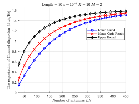
Figure 2: Channel dispersion varies with the number of receiving antennas, $M=2$,$K=10$,$n=50$,$\varepsilon=10^{-6}$.

In Fig.2, we verify the upper and lower bounds derived for the channel dispersion term $Y$ in (31) and (28). We simulated the expected performance of the channel dispersion $V$ for a scenario with blocklength $n=30$ and outage probability $\varepsilon=10^{-6}$, considering UE and EDU number are $K=10$ and $M=2$, respectively.

Simulation results indicate that our derived bounds provide tighter gap limits than Monte Carlo simulations. As the number of receiving antennas $LN$ increases, the system’s SINR significantly improves. It is also observed that the computation of $Y$ stabilizes when the number of antennas exceeds $60$.

Due to the scalability of cell-free systems where the number of receiving antennas is far more than that of transmitting antennas, even in scenarios with high outage probability requirements and short block lengths, the expected value of channel dispersion $Y$ remains significantly lower than the system’s rate. Therefore, our subsequent analysis on SE under finite blocklengths, focusing on the first part of (10), specifically the traditional channel capacity component, will be optimized.

III-B Large-scale Analysis

For analytical convenience and without loss of generality, we adopt the free space path loss model. Assuming the largescale channel model is given by:

$$\beta_{k,l}=d_{k,l}^{-\alpha},$$ (33)

where $d_{k,l}$ represents the distance from the UE $k$ to RRU $l$ and $\alpha$ denotes the path loss exponent; we note that $d_{k,l}>0$ holds under all circumstances.

We aim to maximize UE k’s SE for the large-scale fading coefficient. This problem is formulated using its SE upper or lower bound (27), (30). We use the upper bound to transform the problem into,

$$\max\left\{{\log_{2}}\left({1+{p_{k}}\left\{{\sum\limits_{m=1}^{M}{\sum\limits_{\tilde{l}\in{{\widetilde{\cal L}}_{m,k}}}{{\beta_{\tilde{l},k}}}}}\right\}}\right)\right\}.$$ (34)

Optimizing the form of (34) is challenging due to its complexity. Consider the function $f(x)=x^{-\alpha}$, which is convex because $f^{\prime\prime}(x)=\alpha(\alpha+1)x^{-\alpha-2}>0$ holds for all $x>0$. Therefore, we can apply Jensen’s inequality:

$$\frac{1}{n}\sum_{i=1}^{n}d_{i}{}^{-\alpha}=\frac{1}{n}\sum_{i=1}^{n}f\left(d_{i}\right)\geq f\left(\frac{1}{n}\sum_{i=1}^{n}d_{i}\right)=\left(\frac{1}{n}\sum_{i=1}^{n}d_{i}\right)^{-\alpha}.$$ (35)

To facilitate further processing, we represent the above expression in terms of squared distance,

$$\frac{1}{n}{\sum\limits_{i=1}^{n}{{d_{i}}}^{-\alpha}} =\frac{1}{n}{\sum\limits_{i=1}^{n}{\left({{d_{i}}^{2}}\right)}^{-\frac{\alpha}{2}}}=\frac{1}{n}\sum\limits_{i=1}^{n}f\left({{d_{i}}^{2}}\right)$$ (36)

$$\geq f\left({\frac{1}{n}\sum\limits_{i=1}^{n}{{d_{i}}^{2}}}\right)={\left({\frac{1}{n}\sum\limits_{i=1}^{n}{{d_{i}}^{2}}}\right)^{-\frac{\alpha}{2}}}.$$

According to (36), we can approximate the (34) problem and obtain its lower bound as follows,

$$R_{k}^{{\rm{ub}}}{\rm{}}\geq{\log_{2}}\left({1+{p_{k}}\left\{{\sum\limits_{m=1}^{M}{{{\left({\sum\limits_{\tilde{l}\in{{\widetilde{\cal L}}_{m,k}}}{{d_{k,l}}}^{2}}\right)}^{-\frac{\alpha}{2}}}}}\right\}}\right).$$ (37)

By maximizing its lower bound, the original problem of maximizing SINR is transformed into a problem of minimizing the sum of distances from UE $k$ to all RRUs formulated as follows,

$${\rm{max}}\left\{{\sum\limits_{m=1}^{M}{\sum\limits_{\tilde{l}\in{{\widetilde{\cal L}}_{m,k}}}{{\beta_{\tilde{l},k}}}}}\right\}\to{\rm{min}}\left\{{\sum\limits_{m=1}^{M}{{{\left({\sum\limits_{\tilde{l}\in{{\widetilde{\cal L}}_{m,k}}}{{{d_{k,l}}}^{2}}}\right)}}}}\right\}.$$ (38)

Assuming there are $L$ RRUs, the coordinates of these RRUs are $(x_{1},y_{1}),(x_{2},y_{2}),\cdots,(x_{L},y_{L})$ and the coordinates of UE $k$ are $(x_{k},y_{k})$. The distance from UE $k$ to RRU $l$ is represented as follows,

$$d_{k,l}=\sqrt{\left(x_{k}-x_{l}\right)^{2}+\left(y_{k}-y_{l}\right)^{2}}.$$ (39)

The distance and square of UE $k$ to all RRUs are represented as follows,

$$d_{k}^{2}=\left({\sum\limits_{\tilde{l}\in{{\widetilde{\cal L}}_{m,k}}}{{d_{k,l}}}^{2}}\right)={\sum\limits_{\tilde{l}\in{{\widetilde{\cal L}}_{m,k}}}\left[\left(x_{k}-x_{l}\right)^{2}+\left(y_{k}-y_{l}\right)\right]^{2}}.$$ (40)

Let us consider the presence of an EDU in the scenario, representing traditional centralized processing. In order to minimize $d_{k}^{2}$, we assume that the UEs follow a uniform distribution; therefore, by applying the concavity and convexity of the associative function, taking partial derivatives concerning $x$ and $y$ for the sum of squared distances (40) yields the following expression,

$$\frac{\partial d_{k}^{2}}{\partial x_{k}}=2\sum\limits_{\tilde{l}\in{{\widetilde{\cal L}}_{m,k}}}\left(x_{k}-x_{l}\right),$$ (41)

$$\frac{\partial d_{k}^{2}}{\partial y_{k}}=2\sum\limits_{\tilde{l}\in{{\widetilde{\cal L}}_{m,k}}}\left(y_{k}-y_{l}\right).$$

Based on the necessary conditions for extreme values, we equate the partial derivatives of $d_{k}^{2}$ concerning $x_{k}$ and $y_{k}$ to $0$ as,

$$x_{k}=\frac{1}{n}\sum\limits_{\tilde{l}\in{{\widetilde{\cal L}}_{m,k}}}x_{l},$$ (42)

$$y_{k}=\frac{1}{n}\sum\limits_{\tilde{l}\in{{\widetilde{\cal L}}_{m,k}}}y_{l}.$$

That is, the distance from UE $k$ to all RRUs is the smallest, and only if UE $k$ is located at the center of gravity of all RRUs is the sum of distance (40) the smallest; that is, the lower bound (38) is the largest.

Based on equation (37), we consider the scenario involving multiple EDUs. In this paper, the UEs should be located at the center of gravity of the RRUs in multiple groups of EDUs, while the center of gravity of the UEs should be positioned at the midpoint of the plane. Consequently, each group of RRUs can exhibit a uniform distribution to achieve optimal performance.

However, as the number of EDUs increases, satisfying this requirement becomes more challenging. As a result, achieving a statistically uniform distribution in a higher-dimensional space becomes increasingly tricky. To address this issue, in section IV, we propose a modified graph coloring algorithm that aims to interleave the RRUs between groups as much as possible, considering the random distribution of RRUs. The superiority of the proposed interleaving deployment method has been verified in actual systems, especially in scenarios with OTA reciprocity calibration [43].

III-C RRU correlation method

A genetic algorithm based on the distance relationship between RRUs was proposed to associate EDUs and RRUs [28]. The designed fitting function was,

$$f(x)=\frac{1}{\sum\limits_{p\in\mathcal{P}}{\sum\limits_{q\in\mathcal{Q}}{\cdots}}\sum\limits_{u\in\mathcal{U}}{\sum\limits_{v\in\mathcal{V}}{\left({{d}_{p,q}^{2}}+\cdots+{{d}_{p,v}^{2}}+\cdots+{{d}_{u,v}^{2}}\right)^{1/2}}}},$$ (43)

where ${d}_{p,v}$ is the distance between the $p-$th RRU and the $v-$th RRU, $\mathcal{P},\mathcal{Q},\cdots,\mathcal{U},\mathcal{V}$ is the $p,q,\cdots,u,v$ ’s corresponding RRU grouping of EDUs, and $\mathcal{T}$ is a complete set of all RRUs.

The objective function of the heuristic scheme becomes highly complex with the increase in the number of EDUs, and this heuristic Algorithm has not been theoretically analyzed. Therefore, based on our theoretical analysis above, Assuming the user’s centroid is located at the origin, we use a graph coloring algorithm to reduce the implementation complexity. This scheme’s complexity is significantly reduced compared to the method in the original paper.

III-D Improved Graph Coloring Algorithm

Based on the analysis in the previous section, we know that for multiple groups of EDUs, the RRUs under each group of EDUs should align as closely as possible with the geometric centroid of the UE locations. Since UEs are randomly distributed, we also need to ensure that multiple groups of EDUs satisfy an interleaved random distribution. Therefore, to avoid concentrating RRUs in a small area, we use an improved graph coloring algorithm for association.

In scenarios with a large number of RRUs, especially when the number of RRUs exceeds $100$, the chromosome population designed by traditional genetic algorithms will be huge, leading to enormous complexity [28]. This is an NP-hard combinatorial optimization problem, but the graph coloring algorithm can effectively reduce the implementation complexity of the Algorithm [44]. The graph coloring process indicates a conflict if there is a connection and the two endpoints of the line need to use different coloring schemes, while unconnected RRUs can use the same color. To make the distribution as uniform as possible, we need to fully utilize the number of allocated colors, i.e., the number of EDUs in our case. Previous work has applied graph coloring algorithms to user pilot allocation strategies [45]. Here, we apply an improved graph coloring algorithm to the interleaved deployment of RRUs and EDUs.

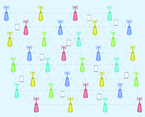
(a) Step N-1:$\delta=0.125$,$M=5$.

(b) Step N:$\delta=0.0625$,$M=2$.

Figure 3: The graph coloring algorithm implementation process, $L=32$,$K=10$.

In scenarios with a large number of RRUs, there will inevitably be cases of unallocated conflicts. Therefore, based on the original graph coloring, we sort the unallocated conflicting RRUs and isolated RRUs according to their distances and connect them sequentially based on the number of remaining colors and distances, solving the problem of isolated points to ensure uniform distribution as much as possible.

The execution process of the improved graph coloring algorithm is shown in Algorithm 1, where the associated distance $\delta$ is continuously updated using the bisection method until the required number of colors meets the number of EDUs.

We use the tabu search method [46] in the color allocation. Tabu search can gradually move towards the minimum value of the function. To avoid cycles and local minima, the tabu list is updated during iteration, reducing the search space and achieving rapid random convergence. The tabu search operation quickly searches for better approximate optimal solutions in a vast solution space.

We connect RRUs of different colors to the same EDU. The example in Fig.3 shows the coloring process of $32$ RRUs with target $2$ EDUs. In the penultimate bisection search, five colors and the connection of RRUs to five EDUs are still required, necessitating further distance refinement. In the next bisection search, only two colors remain for the RRUs, meeting the requirements for the number of EDUs. The RRUs allocated by the improved graph coloring algorithm meet the conditions for maximum interleaving, and calculations are only needed during the initial deployment. Since the centroid positions of all RRUs are located at the system’s origin, it supports infinite scalability. The system’s performance will also improve with the increase in the number of EDUs and the deployment of RRUs.

Algorithm 1 Modified Graph Coloring Algorithm

1:Input: the number of RRU $L$, the number of EDU $M$, distance matrix $\textbf{D}\in\mathbb{R}^{L\times L}$, initial distance scale factor $\delta$.

2:Output: RRU Group $\mathcal{L}_{m}$

3:Every EDU chooses $L_{m}$ RRUs to generate the connect set $\mathcal{L}_{m}$.

4:Generate associate graph matrix $\textbf{D}\in\mathbb{R}^{L\times L}$ through $\mathcal{L}_{m}$.

5:According to D, use the graph coloring algorithm to generate graph results and calculate the target EDU number $n$ based on $\delta$.

6:while $n\neq M$ do

7:  Use the bisection method to update $\delta$.

8:  According to $\delta$, sort the positions by distance based on isolated points and RRUs that are not fully colored and connect to all colors that are fully colored.

9:  Use the graph coloring algorithm to recalculate $n$ and update.

10:end while

TABLE I: Simulation parameters

[b] Simulation Parameters Values Uplink transmission power $200\;\rm{mW}$ Antenna height 10 m Area size $200\times 200\;\rm{m}^{2}$ The number of RRUs, $L$ 100 Number of antennas per RRU, $N$ 4 Number of UEs, $K$ 24 Number of orthogonal pilots,${L_{P}}$ 24 Transmission bandwidth, $B$ 20 MHz Carrier frequency, $f_{c}$ 2 GHz Azimuth angle, $\bar{\varphi}$ (in radians) 15 Elevation angle, $\bar{\theta}$ (in radians) 15 Noise power spectral density, $N_{0}$ $-174\;\rm{dBm/Hz}$

IV Simulation Results Analysis

Based on the analysis in the previous sections, we conduct simulation verification. First, we validate the proposed upper and lower bounds against Monte-Carlo simulation results. Subsequently, we further consider imperfect CSI and the performance of different UE association strategies in the presence of pilot contamination.

IV-A Validation of Upper and Lower Bounds of Average SE in EDU Scenarios

In Fig.4, we validate the perfect CSI by comparing the Monte Carlo simulation results using ZF combining with the theoretical upper and lower bounds. To align as closely as possible with centralized processing in a cell-free system, we refer to the simulation settings in [32]. The system consists of $L=300$ single-antenna RRUs and $K$ UEs uniformly distributed within a specific range. We select a path loss factor of $\alpha=4$.

Fig.4a and Fig.4b simulate the performance for $K=10$ and $K=30$ UEs, respectively. From the gap between the grouped EDUs and theoretical values, we can see that the system performance deteriorates as the number of EDU groups increases. We use the ZF combining scheme as in (9). It can be seen that as the number of UEs increases, the system’s SE continuously improves, and under different numbers of EDUs, the upper and lower bounds of the SE with finite blocklength maintain good tightness. This result verifies the validity of the derived performance upper and lower bounds in (32).

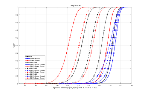
(a) System uplink SE CDF verification, $n=50$, $\varepsilon=10^{-6}$, $K=10$, $L=300$, $N=1$.

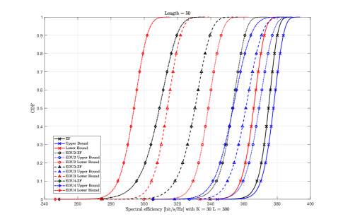
(b) System uplinkSE CDF verification, $n=50$, $\varepsilon=10^{-6}$, $K=30$, $L=300$, $N=1$.

Figure 4: System uplink SE CDF verification.

IV-B Simulation Performance Verification of Interleaved EDU Grouping

In this subsection, we consider more complex scenarios for simulation. We account for imperfect CSI in the uplink system, with system modeling adopting more complex large-scale fading as follows [47],

$$\beta_{k,l}(\textrm{dB})=-30.5-36.7\log_{10}\left({d_{k,l}}\right)+F_{k,l},$$ (44)

where $F_{k,l}$ represents the impact of shadow fading.

Due to the noise power amplification issue in ZF combining, as shown in (8), we also employ a more complex channel combining scheme and consider the impact of multiple antennas, assuming $N=4$. The paper’s simulation parameters are shown in Table I.

Due to channel estimation errors and the limited number of pilots, we consider imperfect CSI. Considering pilot contamination, we further associate UE and RRU. The association information can be obtained at the EDU. We consider the classic scalable association method, dynamic cooperation clusters (DCC), to deal with the pilot contamination in a cell-free scenario [36]. So, the combining vector at the EDU considers the influence of the UE-RRU association matrix, and we adopt the MMSE combining method with the corresponding vector as follows,

$${\bf{v}}_{k,m}=$$ (45)

$${p_{k}}{\left({\sum\limits_{i=1}^{K}{{p_{i}}{{\bf{D}}_{k,m}}\left({{{\widehat{\bf{h}}}_{i,m}}\widehat{\bf{h}}_{i,m}^{\rm{H}}}\right){{\bf{D}}_{k,m}}}+\sigma_{{\rm{UL}}}^{2}{{\bf{I}}_{mN}}}\right)^{-1}}{{\bf{D}}_{k,m}}{\widehat{\bf{h}}_{k,m}},$$

where ${\bf{D}}{k,m}$ represents the association between the $m$-th EDU and user $k$ in the RRU, and ${{\mathbf{h}}{i,k}}={{\hat{\mathbf{h}}}{i,k}}+{{\tilde{\mathbf{h}}}{i,k}}$ represent the channel estimation information and channel estimation error, respectively.

We will compare the interlacing deployment strategy with traditional clustering grouping. The clustering strategy selects the initial position of the RRU as the starting centroid, with the number of EDUs $M$ as the number of cluster centroids, using the final clustering strategy of the RRUs as the corresponding association method. Considering that the centroid positions of the clusters will continuously change during the algorithm implementation, we randomly set the initial cluster centroids and use the final centroids as the deployment locations of the EDUs to minimize clustering error. This approach is common in traditional cellular architectures and CoMP systems, and in this collaborative architecture, we still use clustering as our comparison method. We adopt the classic K-means++ clustering strategy [48], which is used in many scenarios due to its low complexity, fast convergence speed, and good performance [49].

Fig.5 simulates the combining strategy shown in (45), which we refer to as EDU-MMSE and EDU-P-MMSE. Joint MMSE and LP-MMSE (local partial-MMSE) are both exceptional cases.

We further compare the performance of different EDU and RRU association strategies under the scenario of uplink transmission with or without pilot contamination. We simulated the scenario with an outage probability of $10^{-5}$ and a block length of $n=50$. When the number of UE $K$ is greater than the number of pilots $L_{P}$, the DCC strategy is adopted for scalable EDU deployment. Fully centralized processing has the highest implementation complexity and optimal performance, while fully distributed processing has the lowest implementation complexity and the worst performance for each EDU.

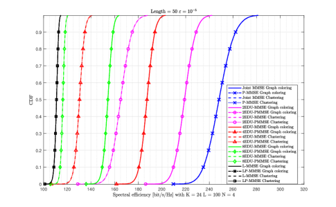
(a) $K=24$,without pilot contamination.

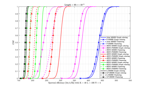
(b) $K=48$,with pilot contamination.

Figure 5: Comparison of upper and lower bounds on the expected spectrum efficiency of uplink systems under different numbers of EDUs, $n=50$, $\varepsilon=10^{-6}$, $L=300$, $N=1$.

As can be seen from Fig.5a, in the absence of pilot contamination, the SE with finite block length is the same when using the DCC strategy and fully centralized deployment, which means that UEs can all be allocated orthogonal pilots. In Fig.5b, the user-centric DCC strategy reduces centralized processing complexity at the cost of some performance loss.

Comparing the performance of the clustering strategy based on the K-means++ method and the interleaving strategy deployment based on the improved graph coloring algorithm, it can be seen that whether or not there is pilot contamination, the SE performance of the interleaving strategy is far superior to that of the clustering strategy under both fully centralized and partial cooperation processing. As the number of EDUs increases, the gap between the clustering strategy and the improved graph coloring method gradually decreases, indicating that the interleaving strategy cannot meet the absolute overlap of the center.

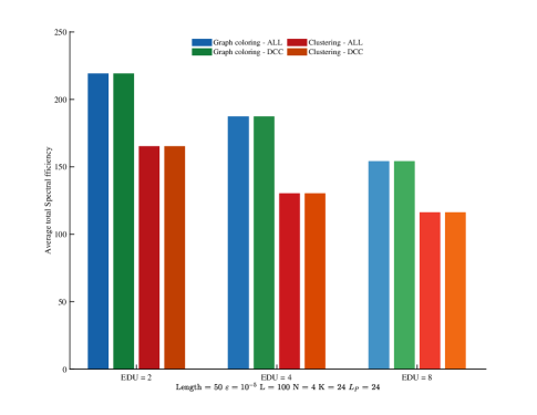
(a) $K=24$,without pilot contamination.

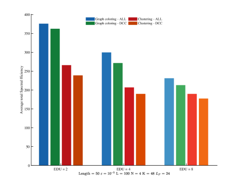
(b) $K=48$,with pilot contamination.

Figure 6: Comparison of upper and lower bounds on the expected SE of uplink systems under different numbers of EDUs, $n=50$, $\varepsilon=10^{-6}$, $L=300$, $N=1$.

In Fig.6, we compare the expected SE of finite blocklengths under scenarios with the number of EDUs being $M=2$, $M=4$, and $M=8$. When the number of EDUs is $M=2$, the SE of finite blocklengths using interleaving deployment can be increased by more than 30% compared to the K-means++ clustering deployment, validating the performance analysis of cooperation in section III. In subsequent simulations in the paper, the deployment method based on the improved graph coloring algorithm interleaving will be used unless otherwise specified.

Remark 4: The interleaving deployment strategy aligns with the system’s actual architectural deployment. This means that in a hotspot area, we can enhance system performance by continuously increasing the deployment density of RRUs and EDUs without considering the regional division of traditional cellular and cell-free RRU clustering deployment.

In Fig.7, we simulate the relationship between the SE of finite block lengths and the outage probability under different numbers of RRUs. The capacity collapse effect persists regardless of the number of antennas. This is because, in finite block length scenarios, the size of channel dispersion $V$ becomes non-negligible as the block length decreases sharply.

However, regardless of the codeword length $n$, the SE of finite blocklengths will increase with the number of system antennas, as proposed by the spatiotemporal exchangeability in the [15].

Yet, as shown in the comparison between Fig.7a and Fig.7b, the number of EDUs is also a key factor affecting the system’s SE under a certain number of receiving RRUs L. Therefore, while ensuring scalability, the system must consider allocating time and spatial resources.

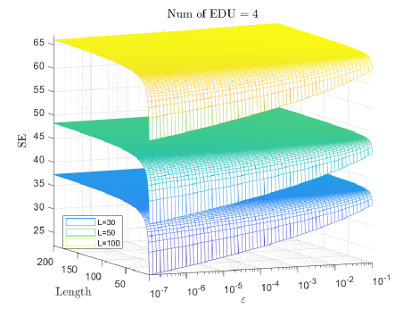
(a) $M=4$.

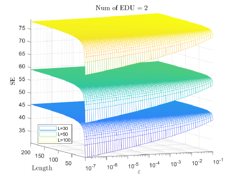
(b) $M=2$.

Figure 7: The relationship between system SE and interruption probability $\varepsilon$ and blocklength $n$ varies with different numbers of RRUs.

The results in Fig.8 simulate the SE of finite blocklengths as the number of UEs $K$ changes under different blocklengths $n$ and various numbers of EDUs $m$. In a scalable cellfree scenario, the system exhibits macro diversity. With the combining scheme in (45), the system’s SINR is relatively large, so the impact of finite block lengths can only be observed in ultra-short block scenarios. The figure shows the blocklength results $n=1$, $n=3$, and $n=5$. In centralized and distributed deployment scenarios with $M=2$ and $M=4$ EDUs, the SE of finite blocklengths increases with the blocklength, but the increase is limited. Therefore, enhancing system performance by increasing the number of block lengths will be limited when spatial resources are sufficient. This also confirms that low-latency requirements are more accessible to meet in cell-free scenarios. Thus, we will focus more on spatial and frequency resource utilization and priority mapping.

The results in Fig.8 show that as the number of UEs $K$ increases, the SE of finite blocklengths also increases approximately linearly. This is due to the large number of antenna ports and layers on the receiving side $L$ of the RRU, which is far more than the number of data streams $K$. Therefore, scalable cell-free will open more possibilities for achieving low latency and high reliability.

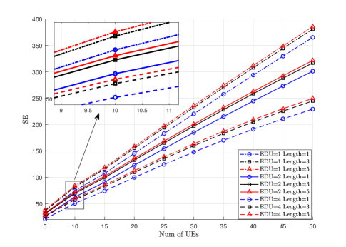
Figure 8: The system SE performance changes with the number of users $K$ under different block lengths $n$ and different numbers of EDUs $M$.

Fig.9 compares the outage probability $\varepsilon$ with different deployment schemes as the block length $n$ changes in a system with a fixed number of RRUs $L=100$ and $N=4$. When centralized processing is adopted, the system’s reliability is the highest. As the number of EDUs $M$ increases, the outage probability $\varepsilon$ rises, and reliability continuously decreases. As the block length $n$ increases, the system’s outage probability tends to a constant value. This is because, with a further increase in blocklength $n$, the finite blocklength rate becomes increasingly close to the traditional channel capacity $C$. At this point, through the outage probability expression calculation, the difference $C-R$ will also tend to be a constant.

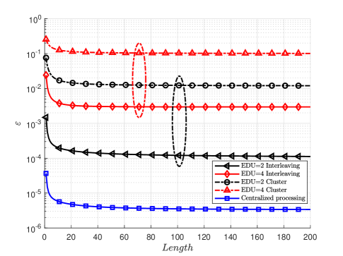
Figure 9: The system outage probability $\varepsilon$ changes with block length $n$ under different merging schemes.

In Fig.10, under the scenario of the number of UEs $K=10$ and a reliability outage probability of $10^{-6}$, the finite blocklength SE is simulated as the number of EDUs $M$ changes. It is assumed that each EDU deploys $20$ RRUs, and each RRU uses the interleaving deployment strategy. The simulation results show that with the increase in the number of EDUs $M$, the SE of finite blocklengths continuously improves and increasingly approximates traditional channel capacity with the increase in blocklength. It can be seen that with the linear increase in deployed antennas, the improvement in SE of finite block lengths is not linear. At this point, the system has more antennas to accommodate more UEs and more data streams.

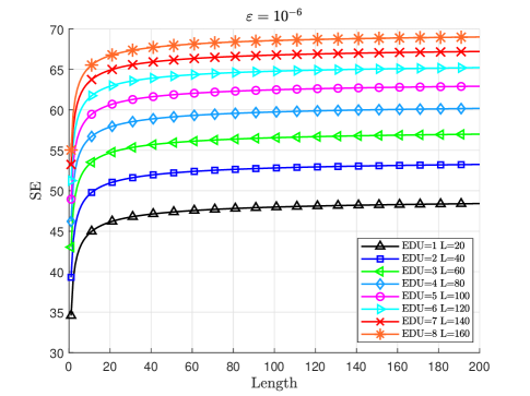
Figure 10: The system SE changes with the number of deployed EDUs $M$, where each EDU includes $20$ RRUs, all adopting the interleaving deployment, with $\varepsilon=10^{-6}$.

Fig.11 simulates the system’s SE as the number of antennas $L/M$ in the EDU changes under the outage probability of $10^{-7}$ in an ultra-short blocklength scenario. The SE of finite block lengths increases with the number of antennas in the EDU. As the block length increases, performance continues to improve.

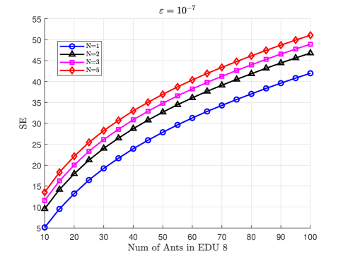
Figure 11: In the ultra-short blocklength scenario, the system SE changes with the number of antennas per EDU, with $\varepsilon=10^{-7}$.

Fig.12 simulates the system’s outage probability $\varepsilon$ as the number of system antennas $LN$ changes in block length $n=50$ and number of UEs $K=10$. It can be seen that as the number of antennas increases, the system’s outage probability continuously decreases. This illustrates the trade-off between scalability and reliability, and we can enhance system performance through more EDU deployments.

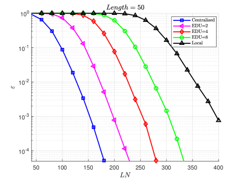
(a) Logarithmic coordinate representation.

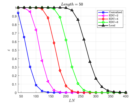
(b) Conventional coordinate representation.

Figure 12: With $K=10$, the system outage probability $\varepsilon$ changes with the number of system antennas $LN$.

Fig.13 simulates the system’s outage probability $\varepsilon$ as the block length $n$ changes under the scenario of the number of UEs $K=10$, with each EDU associated with $20$ RRUs and deploying different numbers of EDUs. The simulation results show that as the block length $n$ increases, the system’s outage probability $\varepsilon$ tends to a constant value. Furthermore, with more EDU deployments, the system’s reliability continuously improves. Therefore, spatial resources can be exchanged for more reliability, and this performance improvement is significant.

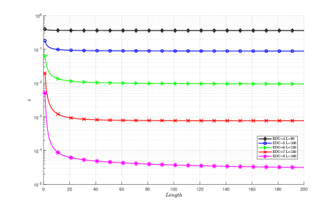
Figure 13: With $K=10$, each EDU associated with $20$ RRUs, the system outage probability $\varepsilon$ changes with blocklength $n$ under different numbers of RRUs.

From the above conclusions, we can see that by utilizing spatial resources, we can effectively exchange for system reliability. Assuming that the block length $n$ is equivalent to the system’s air interface delay, the delay requirements in a scalable cell-free architecture seem to be naturally met. For the system delay, in a scalable cell-free architecture, due to the system’s macro-diversity and high SINR, with the number of receiving antennas far exceeding the number of users, the impact of block length $n$ on system performance is relatively small. Considering the transmission in an OFDM system, there are more subcarrier frequency resources available for mapping. The actual air interface transmission delay mainly focuses on channel information processing. This needs further analysis, especially with partial processing methods to reduce processing complexity.

For example, the multi-agent Q-learning algorithm based on EDU adopted in the paper [28] can find a locally optimal solution under instantaneous channel state information. However, small-scale channel state information significantly affects its implementation complexity. Therefore, the user association strategy under the new cell-free wireless access network still needs further research and consideration. Traditional DCC will result in significant performance loss in multi-EDU scenarios.

V Conclusions

In this paper, we relied on the validated space-time exchange theory in point-to-point transmission to implement uRLLC for scalable Cell-free systems. The SE of a new scalable Cellfree RAN with multiple EDUs was analyzed in the scenario of finite block length. The correlation performance of RRUs under multiple EDUs was examined using a modified graph coloring algorithm for interleaving correlation, which improved system SE under blocklength and error performance constraints. By deploying scalable EDUs, a balance between reliability and latency was achieved and traded off with spatial degrees of freedom (DoF), further expanding and verifying the accuracy of the distributed space-time exchange theory.

References

- [1] A. Dogra, R. K. Jha, and S. Jain, “A survey on beyond 5G network with the advent of 6G: Architecture and emerging technologies,” IEEE Access, vol. 9, pp. 67 512–67 547, 2020.
- [2] Y. Xiaohu, “Shannon theory and future 6G′s technique potentials,” Scientia Sinica Informationis, vol. 50, no. 9, pp. 1377–1394, 2020.
- [3] S. K. Kasi, U. S. Hashmi, M. Nabeel, S. Ekin, and A. Imran, “Analysis of area spectral & energy efficiency in a CoMP-enabled user-centric cloud RAN,” IEEE Transactions on Green Communications and Networking, vol. 5, no. 4, pp. 1999–2015, 2021.
- [4] C. Yang, S. Han, X. Hou, and A. F. Molisch, “How do we design CoMP to achieve its promised potential?” IEEE Wireless Communications, vol. 20, no. 1, pp. 67–74, 2013.
- [5] B. Zong, C. Fan, X. Wang, X. Duan, B. Wang, and J. Wang, “6G technologies: Key drivers, core requirements, system architectures, and enabling technologies,” IEEE Vehicular Technology Magazine, vol. 14, no. 3, pp. 18–27, 2019.
- [6] X. You, C.-X. Wang, J. Huang, X. Gao, Z. Zhang, M. Wang, Y. Huang, C. Zhang, Y. Jiang, J. Wang et al., “Towards 6G wireless communication networks: Vision, enabling technologies, and new paradigm shifts,” Scientia Sinica Informationis, vol. 64, no. 1, pp. 1–74, 2021.
- [7] X. You, Y. Huang, S. Liu, D. Wang, J. Ma, C. Zhang, H. Zhan, C. Zhang, J. Zhang, Z. Liu, J. Li, M. Zhu, J. You, D. Liu, Y. Cao, S. He, G. He, F. Yang, Y. Liu, J. Wu, J. Lu, G. Li, X. Chen, W. Chen, and W. Gao, “Toward 6G extreme connectivity: Architecture, key technologies and experiments,” IEEE Wireless Communications, vol. 30, no. 3, pp. 86–95, 2023.
- [8] C.-X. Wang, X. You, X. Gao, X. Zhu, Z. Li, C. Zhang, H. Wang, Y. Huang, Y. Chen, H. Haas et al., “On the road to 6g: Visions, requirements, key technologies, and testbeds,” IEEE Communications Surveys & Tutorials, vol. 25, no. 2, pp. 905–974, 2023.
- [9] J. Park, S. Samarakoon, H. Shiri, M. K. Abdel-Aziz, T. Nishio, A. Elgabli, and M. Bennis, “Extreme URLLC: Vision, challenges, and key enablers,” arXiv preprint arXiv:2001.09683, 2020.
- [10] A. Pourkabirian, M. S. Kordafshari, A. Jindal, and M. H. Anisi, “A vision of 6G URLLC: Physical-layer technologies and enablers,” IEEE Communications Standards Magazine, vol. 8, no. 2, pp. 20–27, 2024.
- [11] M. U. A. Siddiqui, H. Abumarshoud, L. Bariah, S. Muhaidat, M. A. Imran, and L. Mohjazi, “URLLC in beyond 5G and 6G networks: An interference management perspective,” IEEE Access, vol. 11, pp. 54 639–54 663, 2023.
- [12] C. Yue, V. Miloslavskaya, M. Shirvanimoghaddam, B. Vucetic, and Y. Li, “Efficient decoders for short block length codes in 6G URLLC,” IEEE Communications Magazine, vol. 61, no. 4, pp. 84–90, 2023.
- [13] X. You, “6G extreme connectivity via exploring spatiotemporal exchangeability,” Science China Information Sciences, vol. 66, no. 3, p. 130306, 2023.
- [14] X. You, C. Zhang, B. Sheng, Y. Huang, C. Ji, Y. Shen, W. Zhou, and J. Liu, “Spatiotemporal 2-D channel coding for very low latency reliable MIMO transmission,” in 2022 IEEE Globecom Workshops (GC Wkshps). IEEE, 2022, pp. 473–479.
- [15] X. You, B. Sheng, Y. Huang, W. Xu, C. Zhang, D. Wang, P. Zhu, and C. Ji, “Closed-form approximation for performance bound of finite blocklength massive MIMO transmission,” IEEE Transactions on Communications, 2023.
- [16] F. Ye, X. You, J. Li, C. Zhang, and C. Ji, “Explicit performance bound of finite blocklength coded MIMO: Time-domain versus spatiotemporal channel coding,” arXiv preprint arXiv:2406.13922, 2024.
- [17] H. Q. Ngo, A. Ashikhmin, H. Yang, E. G. Larsson, and T. L. Marzetta, “Cell-free massive MIMO versus small cells,” IEEE Transactions on Wireless Communications, vol. 16, no. 3, pp. 1834–1850, 2017.
- [18] F. Riera-Palou, G. Femenias, A. G. Armada, and A. Pérez-Neira, “Clustered cell-free massive MIMO,” in 2018 IEEE Globecom Workshops (GC Wkshps). IEEE, 2018, pp. 1–6.
- [19] M. Matthaiou, H. Q. Ngo, P. J. Smith, H. Tataria, and S. Jin, “Massive MIMO with a generalized channel model: Fundamental aspects,” in 2019 IEEE 20th International Workshop on Signal Processing Advances in Wireless Communications (SPAWC). IEEE, 2019, pp. 1–5.
- [20] X. You, D. Wang, and J. Wang, Distributed MIMO and Cell-Free Mobile Communication. Springer, 2021.
- [21] Q. Peng, H. Ren, C. Pan, N. Liu, and M. Elkashlan, “Resource allocation for uplink cell-free massive MIMO enabled URLLC in a smart factory,” IEEE Transactions on Communications, vol. 71, no. 1, pp. 553–568, 2022.
- [22] Q. Peng, H. Ren, C. Pan, N. Liu, and M. Elkashlan, “Resource allocation for cell-free massive MIMO-enabled URLLC downlink systems,” IEEE Transactions on Vehicular Technology, vol. 72, no. 6, pp. 7669–7684, 2023.
- [23] U. Bucci, D. Cassioli, and A. Marotta, “Performance of spatially diverse URLLC and eMBB traffic in cell free massive MIMO environments,” IEEE Transactions on Network and Service Management, 2023.
- [24] A. A. Nasir, H. D. Tuan, H. Q. Ngo, T. Q. Duong, and H. V. Poor, “Cell-free massive MIMO in the short blocklength regime for URLLC,” IEEE Transactions on Wireless Communications, vol. 20, no. 9, pp. 5861–5871, 2021.
- [25] A. Lancho, G. Durisi, and L. Sanguinetti, “Cell-free massive MIMO for URLLC: A finite-blocklength analysis,” IEEE Transactions on Wireless Communications, vol. 22, no. 12, pp. 8723–8735, 2023.
- [26] H. Peng, Qihao and Ren, M. Dong, M. Elkashlan, K.-K. Wong, and L. Hanzo, “Resource allocation for cell-free massive MIMO-aided URLLC systems relying on pilot sharing,” IEEE Journal on Selected Areas in Communications, vol. 41, no. 7, pp. 2193–2207, 2023.
- [27] E. Björnson and L. Sanguinetti, “Making cell-free massive MIMO competitive with MMSE processing and centralized implementation,” IEEE Transactions on Wireless Communications, vol. 19, no. 1, pp. 77–90, 2019.
- [28] Y. Cao, Z. Zhang, X. Xia, P. Xin, D. Liu, K. Zheng, M. Lou, J. Jin, Q. Wang, D. Wang et al., “From ORAN to cell-free RAN: Architecture, performance analysis, testbeds and trials,” arXiv preprint arXiv:2301.12804, 2023.
- [29] A. Papazafeiropoulos, P. Kourtessis, M. Di Renzo, S. Chatzinotas, and J. M. Senior, “Performance analysis of cell-free massive MIMO systems: A stochastic geometry approach,” IEEE Transactions on Vehicular Technology, vol. 69, no. 4, pp. 3523–3537, 2020.
- [30] M. Zbairi, I. Ez-Zazi, and M. Arioua, “Uplink spectral efficiency of cell free massive MIMO based on stochastic geometry approach,” in 2021 4th International Conference on Advanced Communication Technologies and Networking (CommNet). IEEE, 2021, pp. 1–6.
- [31] Z. Chen and E. Björnson, “Channel hardening and favorable propagation in cell-free massive MIMO with stochastic geometry,” IEEE Transactions on Communications, vol. 66, no. 11, pp. 5205–5219, 2018.
- [32] P. Liu, K. Luo, D. Chen, and T. Jiang, “Spectral efficiency analysis of cell-free massive MIMO systems with zero-forcing detector,” IEEE Transactions on Wireless Communications, vol. 19, no. 2, pp. 795–807, 2019.
- [33] J. Wang and L. Dai, “Asymptotic rate analysis of downlink multi-user systems with co-located and distributed antennas,” IEEE Transactions on Wireless Communications, vol. 14, no. 6, pp. 3046–3058, 2015.
- [34] H. Q. Ngo, E. G. Larsson, and T. L. Marzetta, “Energy and spectral efficiency of very large multiuser MIMO systems,” IEEE Transactions on Communications, vol. 61, no. 4, pp. 1436–1449, 2013.
- [35] D. Wang, X. You, Y. Huang, W. Xu, J. Li, P. Zhu, Y. Jiang, Y. Cao, X. Xia, Z. Zhang et al., “Full-spectrum cell-free RAN for 6G systems: system design and experimental results,” Science China Information Sciences, vol. 66, no. 3, pp. 1–14, 2023.
- [36] E. Björnson and L. Sanguinetti, “Scalable cell-free massive MIMO systems,” IEEE Transactions on Communications, vol. 68, no. 7, pp. 4247–4261, 2020.
- [37] Y. Polyanskiy, H. V. Poor, and S. Verdú, “Channel coding rate in the finite blocklength regime,” IEEE Transactions on Information Theory, vol. 56, no. 5, pp. 2307–2359, 2010.
- [38] W. Yang, G. Durisi, T. Koch, and Y. Polyanskiy, “Quasi-static multiple-antenna fading channels at finite blocklength,” IEEE Transactions on Information Theory, vol. 60, no. 7, pp. 4232–4265, 2014.
- [39] S. Schiessl, J. Gross, M. Skoglund, and G. Caire, “Delay performance of the multiuser MISO downlink under imperfect CSI and finite-length coding,” IEEE Journal on Selected Areas in Communications, vol. 37, no. 4, pp. 765–779, 2019.
- [40] H. Ren, C. Pan, Y. Deng, M. Elkashlan, and A. Nallanathan, “Joint pilot and payload power allocation for massive-MIMO-enabled URLLC IIoT networks,” IEEE Journal on Selected Areas in Communications, vol. 38, no. 5, pp. 816–830, 2020.
- [41] J. Zhang, J. Zhang, E. Björnson, and B. Ai, “Local partial zero-forcing combining for cell-free massive MIMO systems,” IEEE Transactions on Communications, vol. 69, no. 12, pp. 8459–8473, 2021.
- [42] L. Zhang, P. Zhu, J. Li, and J. Cao, “Downlink ergodic rate analysis of das with linear beamforming under pilot contamination,” in 2017 9th International Conference on Wireless Communications and Signal Processing (WCSP). IEEE, 2017, pp. 1–6.
- [43] Y. Cao, P. Wang, K. Zheng, X. Liang, D. Liu, M. Lou, J. Jin, Q. Wang, D. Wang, Y. Huang et al., “Experimental performance evaluation of cell-free massive MIMO systems using COTS RRU with OTA reciprocity calibration and phase synchronization,” IEEE Journal on Selected Areas in Communications, vol. 41, no. 6, pp. 1620–1634, 2023.
- [44] H. Liu, J. Zhang, S. Jin, and B. Ai, “Graph coloring based pilot assignment for cell-free massive MIMO systems,” IEEE Transactions on Vehicular Technology, vol. 69, no. 8, pp. 9180–9184, 2020.
- [45] X. Zhu, L. Dai, and Z. Wang, “Graph coloring based pilot allocation to mitigate pilot contamination for multi-cell massive MIMO systems,” IEEE Communications Letters, vol. 19, no. 10, pp. 1842–1845, 2015.
- [46] R. Marappan and G. Sethumadhavan, “Solution to graph coloring using genetic and tabu search procedures,” Arabian Journal for Science and Engineering, vol. 43, pp. 525–542, 2018.
- [47] E. Björnson, J. Hoydis, L. Sanguinetti et al., “Massive MIMO networks: Spectral, energy, and hardware efficiency,” Foundations and Trends® in Signal Processing, vol. 11, no. 3-4, pp. 154–655, 2017.
- [48] D. Arthur and S. Vassilvitskii, “k-means++: The advantages of careful seeding,” Stanford, Tech. Rep., 2006.
- [49] Q. N. Le, V.-D. Nguyen, O. A. Dobre, N.-P. Nguyen, R. Zhao, and S. Chatzinotas, “Learning-assisted user clustering in cell-free massive MIMO-NOMA networks,” IEEE Transactions on Vehicular Technology, vol. 70, no. 12, pp. 12 872–12 887, 2021.