Complexity-Aware Training of Deep Neural Networks for Optimal Structure Discovery

Abstract

We propose a novel algorithm for combined unit/filter and layer pruning of deep neural networks that functions during training and without requiring a pre-trained network to apply. Our algorithm optimally trades-off learning accuracy and pruning levels while balancing layer vs. unit/filter pruning and computational vs. parameter complexity using only three user-defined parameters, which are easy to interpret and tune. The optimal network structure is found as the solution of a stochastic optimization problem over the network weights and the parameters of variational Bernoulli distributions for $0/1$ Random Variables scaling the units and layers of the network. Pruning occurs when a variational parameter converges to 0 rendering the corresponding structure permanently inactive, thus saving computations during training and prediction. A key contribution of our approach is to define a cost function that combines the objectives of prediction accuracy and network pruning in a computational/parameter complexity-aware manner and the automatic selection of the many regularization parameters. We show that the solutions of the optimization problem to which the algorithm converges are deterministic networks. We analyze the ODE system that underlies our stochastic optimization algorithm and establish domains of attraction around zero for the dynamics of the network parameters. These results provide theoretical support for safely pruning units/filters and/or layers during training and lead to practical pruning conditions. We evaluate our method on the CIFAR-10/100 and ImageNet datasets using ResNet architectures and demonstrate that our method improves upon layer only or unit only pruning and favorably competes with combined unit/filter and layer pruning algorithms requiring pre-trained networks with respect to pruning ratios and test accuracy.

Keywords: Neural networks, Structured pruning, Bayesian model selection, Variational inference

1 Introduction

Deep neural networks (DNNs) have been shown to be very effective in a variety of machine learning tasks, such as natural language processing, object detection, semantic image segmentation and reinforcement learning [1, 2, 3]. In recent years, it has been widely accepted that these large-scale DNNs generally outperform their smaller counterparts if trained correctly. Residual architectures such as ResNets [4, 5] together with Batch Normalization [6] can be trained effectively even when the number of layers are well into the hundreds. However, such large-scale and resource-consuming models are challenging to train and more so to deploy if the available hardware is limited, e.g., on mobile devices.

Neural network pruning [7, 8] has been used to reduce the size of over-parameterized NNs by identifying and removing redundant structures without affecting their prediction accuracy appreciably. While at first such methods pruned individual weights [7], in more recent years structured unit/filter pruning [9, 10, 11, 12, 13] and layer pruning [14, 15, 16] have been found to be more effective. In addition, contributing to the success of pruning methods, it is often found that training larger networks and pruning them to smaller size leads to superior performance compared to just training the smaller models from a fresh initialization [8, 17, 18, 16].

However, most existing pruning methods come with certain limitations that make them inconvenient to use in practice. For example, many methods require pre-trained networks and rely on expensive iterative pruning and retraining schemes or require significant effort in tuning hyperparameters. Moreover, most pruning methods focus on either unit/filter or layer pruning and existing literature on effectively combining the two is limited. While in principle a variety of unit/filter and layer pruning methods can be applied successively to obtain a NN that is pruned in both dimensions, it is often unclear and hardware dependent to what extent layer pruning, which reduces the sequential workload of computing through layers, is more beneficial than unit/filter pruning, which reduces the parallelizable computations within a layer. Moreover, the effect of pruning on reducing the computational load or floating point operations (FLOPS) vs. the number of network parameters and the memory footprint of a NN needs to be distinguished and regulated.

1.1 Related Work

Pruning Pre-Trained Networks: Such pruning methods require pre-trained networks that are expensive to obtain when transfer learning is not applicable. Furthermore, they compress the network by iterating between pruning and fine-tuning or knowledge distillation phases which add additional computational load.

In this group and for layer pruning, Discrimination based Block-level Pruning (DBP) [15] and also [14] identify and remove layers from feed-forward and residual DNNs by analyzing the output features of different layers. Linear classifiers are trained to generate predictions from features extracted at different intermediate layers and identify the layers that provide minor contributions to the network’s performance. Other approaches aim to prune the least important residual blocks from a NN towards achieving a desired pruning ratio. For example, in [19] each such block is followed by a Batch Normalization (BN) layer and can be effectively removed by setting every factor of the BN layer to zero. The impact to the loss function is approximated using first-order gradients to define an importance score for each residual block; the method prunes the blocks with the lowest score.

A unit/filter pruning method requiring pre-trained networks is for example Filter Thresholding (FT) [9] that uses the Euclidean norm of the fan-out weight vector in fully-connected layers or the Frobenius norm of each kernel matrix in convolutional layers as a score to prune the corresponding unit or filter from the network. This method simply keeps the units/filters with the largest norm until the desired sparsity level is met. SoftNet [10] is similar to FT [9] but uses the absolute-value norm of the weights corresponding to a unit in a layer as the score. Also ThiNet [20] iteratively prunes feature maps or units, whose removal leads to the least absolute error in the pre-activation of the subsequent layer, until a desired pruning level is achieved.

Simultaneous Training and Pruning: These methods carry out the pruning simultaneously with the initial network training and hence do not require pre-trained networks; also, they hold the potential for reducing the computational load of training as well as that of inference. [21, 22, 23] introduce scaling factors at the output of specific structures such as neurons, group or residual blocks of the network and place sparsity regularization in form of the $\mathcal{L}_{1}$-norm on them; as a result, some of these factors are forced to zero during training and the corresponding structure is removed from the network. Network slimming [23] uses the scaling factors of BN layers as an importance metric to prune units/filters from the network. Again, $\mathcal{L}_{1}$-norm regularization is placed on the factors and channels are pruned if the factors are small as determined by a global threshold for the whole network.

Bayesian variational techniques together with sparsity promoting priors have been also employed for neural network unit/filter pruning [18, 24, 25, 13] and layer pruning [26, 16]. Such methods typically employ Gaussian scale mixture priors, which are zero mean normal probability density functions (PDF’s) with variance (scale) given by another RV. A notable prior in this class is the spike-and-slab prior, which uses only two scales. Dropout [27] with a Bernoulli distribution has been interpreted as imposing a spike-and-slab PDF on the weights of a NN [28, 18]. [13] and [16] employ Bernoulli scale RVs for each unit/filter and layer of the network, respectively and learn their distributions concurrently with the network’s weights. To overcome the challenge of avoiding premature pruning of structures due to a possible poor initialization of the weights and the starting architecture, [13] proposes the “flattening” hyper-prior for the parameters of the scale RV. Further, it is shown in [16] that the same hyper-prior leads to an optimization problem with solutions at which all Bernoulli parameters are either $0$ or $1$ in each layer of the network and hence training the NN to obtain such a solution yields an optimally pruned deterministic network.

Combined Layer and Unit/Filter Pruning: Existing methods that perform layer and unit/filter pruning concurrently are less available. [29] combines the layer pruning method DBP of [15] with the unit/filter-wise network slimming method of [23] into an iterative pruning and fine-tuning method that requires a pre-trained NN as input. [29] makes the modification to [23] that the pruning threshold for units is set locally in each layer rather than globally and uses down-sampled input images, effectively modifying the dataset, to further improve the networks efficiency. [30] jointly prunes layers and units/filters starting from a pre-trained network and by introducing soft masks to scale the outputs of different structures of the NN. [30] employs an objective function that also promotes sparsity regularization and aims to align the output of the baseline model with the one of the masked network; the resulting optimization problem is solved via generative adversarial learning techniques whereby the scaling factors in the soft masks are forced to zero to effect pruning. The methods of [29, 30] do not directly address the specific challenges of combined layer and unit pruning, brought up earlier.

1.2 Overview of the Proposed Algorithm

In this work, we propose a simultaneous learning and pruning algorithm that effectively combines the unit/filter pruning from [13] and the layer pruning from [16] to address the raised difficulties of balancing layer vs. unit pruning as well as FLOPS vs. parameter pruning. Our method is capable of obtaining a compact sub-network with state-of-the art performance via a single training run that does not require pre-trained weights or iterative re-training. There are several key contributions in this work distinguishing it from and further developing the previous literature. While [13] and [16] work well and robustly for a wide range of the scale RVs hyperparameters common in all layers, it was observed in several experiments that choosing them layer-wise throughout the network improves performance. However, for deep NNs with many layers tuning these hyperparameters by hand becomes infeasible. To overcome this issue, the algorithm proposed here provides a novel approach to automatically select such layer-wise regularization parameters based on the expected computational and memory complexity of the neural network. More specifically, we relate the expected number of FLOPS as well as the number of parameters of the network to the scale RVs parameters of units and layers. Then, the regularization parameters are chosen dynamically during training such that the evolving expected complexity appears as a term in the cost function of the optimization problem. The latter now explicitly integrates the objectives of prediction accuracy and of combined layer and unit pruning in a complexity-aware way. Thus, our approach furnishes a framework to determine optimal NN structures from both a performance and size objective. Furthermore, the proposed method relies on only three easily interpretable hyperparameters that i) control the general pruning level, ii) regulate layer vs. unit pruning and iii) trade off computational load vs. the number of parameters of the network, addressing all previously discussed challenges of combined layer and unit pruning.

Similar to [13, 16], we introduce Bernoulli RVs for the layers and units of the network and use a projected gradient descent algorithm to learn the Bernoulli parameters of the variational posterior distributions. However, the theoretical analysis in [13, 16] of their respective training/pruning algorithms, which was used to find provable pruning conditions, is shown to fail when layer and unit pruning are combined, necessitating a new approach. Specifically, in the setting of combined layer and unit/filter pruning convergence needs to be shown to a set, representing possible solutions of the optimization problem corresponding to either layer or unit/filter pruning, rather than a single equilibrium point. Using Lyapunov Stability theory we prove conditions under which the scale RVs and the weights of a unit/filter or layer of the NN converge to their elimination and can be safely removed during training (Theorem 5.1 and Theorem 5.2). These theoretical results lead to practical pruning conditions implemented in our algorithm. In addition, we show that the resulting pruned networks are always deterministic and therefore extend one of the main results of [16] to the combined pruning case (Theorem 3.1).

The remainder of this paper is arranged as follows. In Section 2, we present the statistical modeling that forms the basis of the pruning approach and formulate the resulting optimization problem. Section 3 presents the main ideas in combining unit and layer pruning to address its challenges and provides the theoretical characterization of the solutions of the optimization problem. In Section 4, we summarize the proposed concurrent learning/pruning algorithm. Convergence results supporting the pruning process are provided in Section 5. In Section 6, we present simulations on standard machine learning problems to demonstrate the effectiveness and ease of use of our method and compare it to competing combined layer and unit pruning methods. Finally, Section 7 concludes the paper.

Notation: We use the superscript $l$ to distinguish parameters or variables of the $l$th layer of a neural network. We use $n$ in indexing such as $x(n)$ to denote iteration count. Also $\lVert\cdot\rVert$ denotes the Euclidean norm of a vector or the Frobenius norm of a matrix, $M^{T}$ the transpose of a matrix (or vector), and $\operatorname{\mathbb{E}}[\cdot]$ taking expectation with respect to the indicated random variables. Other notations are introduced before their use.

2 Problem Formulation

We consider a residual network structure obtained by cascading the blocks depicted in Figure 1. The part of the block inside the dashed box can be repeated $M$ times to yield many commonly used structures, such as the various ResNet networks. In such a case, consecutive weights (convolutions) should be replaced by a single weight (convolution). The theoretical part of this work assumes for simplicity fully-connected layers as shown and $M=1$, but the results can be readily extended to structures with $M>1$ and convolutional layers as discussed later and demonstrated by our simulations. This structure yields a network with $L$ residual blocks realizing mappings $\hat{y}=NN(x;W,\Xi)$ as follows:

$$\begin{split}z^{1}&=x;\\ \bar{z}^{l}&=\xi_{2}^{l}\odot h^{l}(z^{l});\quad z^{l+1}=\xi_{B}^{l}\cdot\left[W^{l}_{2}\left(\xi_{1}^{l}\odot a^{l}\left(W^{l}_{1}\bar{z}^{l}+b_{1}^{l}\right)\right)\right]+W_{3}^{l}\bar{z}^{l}+b_{3}^{l};\quad\quad\text{for}\quad l=1\dots L,\\ \hat{y}&=h^{L+1}(z^{L+1}).\end{split}$$ (1)

Figure 1: The network structure considered in this work (see (1)). $z^{l}$ are input features, $a^{l},h^{l}$ the activation functions and $W_{1}^{l},W_{2}^{l}$ and $W_{3}^{l}$ network weights. The scalar Bernoulli RV $\xi_{B}^{l}$ multiplies the output of the block $W_{1}^{l}-a^{l}-W_{2}^{l}$ and the vector valued Bernoulli RVs $\xi_{1}^{l}$ and $\xi_{2}^{l}$ mutliply their corresponding signals element-wise. Bias weights are not shown for simplicity.

In this model, $\xi_{B}^{l}\sim Bernoulli(\pi^{l})$ are scalar discrete Bernoulli $0/1$ random variables with parameter $\pi_{B}^{l}$. Also, $\xi_{1}^{l}\sim Bernoulli(\pi_{1}^{l})$ and $\xi_{2}^{l}\sim Bernoulli(\pi_{2}^{l})$ are vector valued Bernoulli RVs with parameter $\pi_{1}^{l}$ and $\pi_{2}^{l}$, respectively. The matrices $W_{1}^{l},W_{2}^{l},W_{3}^{l},b_{1}^{l}$, $b_{3}^{l}$ are of appropriate dimensions and the element-wise activation functions $a^{l}(\cdot)$ and $h^{l}(\cdot)$ are assumed to be twice continuously differentiable and satisfy $a^{l}(0)=0$ for $l=1\dots L$ and $h^{l}(0)=0$ for $l=1\dots L+1$. To obtain a non-residual output layer, we can remove the nonlinear path of the last block leading to $\hat{y}=h^{L+1}(W_{3}^{L}\bar{z}_{L}+b_{3}^{L})$. $h^{1}(\cdot)$ is typically the identity function. To simplify the notation, we absorb the additive bias vectors $b^{l}_{1}$ and $b^{l}_{3}$ into the weight matrices $W^{l}_{1}$ and $W^{l}_{3}$, respectively as an additional last column and append their inputs with a unity last element. We denote collectively $W_{1}^{l},W_{2}^{l},W_{3}^{l}$, $l=1,\ldots,L$ by $W$. Further, we collect $\xi_{B}^{l}$, $\pi_{B}^{l}$, $l=1,\ldots,L$ in $\Xi_{B}$ and $\Pi_{B}$ as well as $\xi_{j}^{l}$, $\pi_{j}^{l}$, $l=1,\ldots,L$ in $\Xi_{j}$ and $\Pi_{j}$ for $j=1,2$. Lastly $\Xi_{B},\Xi_{1},\Xi_{2}$ together are denoted by $\Xi$ and $\Pi_{B},\Pi_{1},\Pi_{2}$ by $\Pi$.

Realizations of the Bernoulli $\xi_{B}^{l}$ RVs implement layer-sub-networks of structure (1), where the $l$th nonlinear path is active with probability $\pi_{B}^{l}$. Specifically if $\xi_{B}^{l}=0$ in block $l$, its nonlinear path is inactive and its output is calculated from the linear path only. Similarly, realizations of $\xi_{1}^{l}$ and $\xi_{2}^{l}$ RVs implement unit/filter-sub-networks, where a unit/filter is active with probability $\pi_{1}^{l}$ and $\pi_{2}^{l}$, respectively.

2.1 Statistical Modeling

Given a dataset $\mathcal{D}=\{(x_{i},y_{i})\}_{i=1}^{N}$, where $x_{i}\in\mathbb{R}^{m}$ are input patterns and $y_{i}\in\mathbb{R}^{n}$ are the corresponding target values, the goal is to learn all three sets of weights $W$ and appropriate parameters $\Pi$ for the prior distributions of the RVs $\Xi$ for the NN in (1).

We have already assumed Bernoulli prior distributions $p(\xi_{B}^{l}\mid\pi_{B}^{l})$ for the RVs $\xi_{B}^{l}$’s in $\xi_{B}$ as well as vector valued Bernoulli prior distributions $p(\xi_{1}^{l}\mid\pi_{1}^{l})$ for the RVs $\xi_{1}^{l}$’s in $\Xi_{1}$ and $p(\xi_{2}^{l}\mid\pi_{2}^{l})$ for the RVs $\xi_{2}^{l}$’s in $\Xi_{2}$. The weights in $W$ receive Normal prior distributions $p(W^{l}\mid\lambda)\sim\mathcal{N}\big{(}0,\lambda^{-1}\mathbf{I}\big{)}$. Then, the overall prior distribution factorizes as follows

$$p(W,\Xi\mid\Pi,\lambda)=p(W\mid\lambda)\cdot p(\Xi\mid\Pi)=\prod_{l=1}^{L}p(W^{l}\mid\lambda)\cdot p(\xi_{B}^{l}\mid\pi_{B}^{l})\cdot p(\xi_{1}^{l}\mid\pi_{1}^{l})\cdot p(\xi_{2}^{l}\mid\pi_{2}^{l}).$$

Next, we place flattening hyper-priors $p(\pi_{B}^{l}\mid\gamma_{B})$ and $p(\pi_{j}^{l}\mid\gamma_{j}),\,\,j=1,2$ on the variables $\Pi$. The flattening hyper-prior was introduced in [13] and is defined as

$$p(\pi\mid\gamma)=\frac{\gamma-1}{\log\gamma}\cdot\frac{1}{1+(\gamma-1)(1-\pi)},\quad 0<\gamma<1$$

for $\pi=\pi_{B}^{l}$ or $\pi_{j}^{l},\,j=1,2$ , $l=1,\ldots,L$. Here, $p(\Pi|\Gamma)$ is taken to be the product of such terms over the layers and units of the network. This hyper-prior encourages the convergence of elements of $\pi_{1}^{l}$ or $\pi_{2}^{l}$ to zero, and therefore the removal of features/filters, in a manner avoiding the premature pruning of network substructures. In [13], such substructures are individual units only and in [16] are layers only, while this work combines both to obtain a combined layer and unit/filter pruning scheme.

2.2 Variational Model Fitting

By combining the NN’s statistical model $p(Y\mid X,W,\Xi)$ with the prior distributions and integrating out $\Xi$, we obtain the posterior

$$p(W,\Pi\mid Y,X,\lambda,\gamma) \propto p(Y\mid X,W,\Pi)\cdot p(W\mid\lambda)\cdot p(\Pi\mid\gamma),$$

and select the parameters $\Pi$ and $W$ via Maximum a Posteriori (MAP) estimation:

$$\max_{W,\Pi}\left[\log p(Y\mid X,W,\Pi)+\log p(W\mid\lambda)+\log p(\Pi\mid\gamma)\right].$$ (2)

For deep neural networks the exact $p(Y\mid X,W,\Pi)$ in (2) resulting from integrating out $\Xi$ is intractable, necessitating the approximation of the posterior distribution of $\Xi$. To this end, we introduce the variational posterior

$$q(\Xi\mid\Theta)\sim Bernoulli(\Theta),$$

and recall the Variational lower bound or ELBO (see e.g. [31, Chapter 10])

$$\log p(Y\mid X,W,\Pi)\geq\int q(\Xi\mid\Theta)\log p(Y\mid X,W,\Xi)\mathop{}\!\mathrm{d}\Xi-\text{KL}\big{(}q(\Xi\mid\Theta)\;\|\;p(\Xi\mid\Pi)\big{)}\equiv L_{B}(\Theta,W,\Pi),$$

where $KL(\cdot\mid\cdot)$ denotes the Kullback-Leibler divergence. Then, after replacing the intractable evidence $\log p(Y\mid X,W,\Pi)$ in (2) with the ELBO $L_{B}(\Theta,W,\Pi)$, we obtain the maximization objective:

$$\begin{split}\max_{W,\Pi,\Theta}\int q(\Xi\mid\Theta)\log p(Y\mid X,W,\Xi)\mathop{}\!\mathrm{d}\Xi-\text{KL}\big{(}q(\Xi\mid\Theta)\;\|\;p(\Xi\mid\Pi)\big{)}+\log p(W\mid\lambda)+\log p(\Pi\mid\gamma).\end{split}$$ (3)

Next, in the spirit of [32] and [13], we first maximize the main objective (3) with respect to $\Pi$ by equivalently minimizing:

$$\min_{\Pi}J_{tot}(\Pi)\equiv\text{KL}\big{(}q(\Xi\mid\Theta)\;\|\;p(\Xi\mid\Pi)\big{)}-\log p(\Pi\mid\gamma.)$$ (4)

Since $J_{tot}(\Pi)$ in (4) factorizes over the unit and layer probabilities, we can express $J_{tot}(\Pi)=\sum_{(\pi,\theta)}J(\pi;\theta)$ with

$$J(\pi;\theta)=(1-\theta)\log\frac{1-\theta}{1-\pi}+\theta\log\frac{\theta}{\pi}+\log\left(1+(\gamma-1)(1-\pi)\right).$$

It was shown in [13] for the flattening hyper-prior that the optimal $\pi$ is given by:

$$\pi^{\star}=\pi^{\star}(\theta)=\arg\min_{\pi}J(\pi\;\theta)=\frac{\gamma\theta}{1+\theta(\gamma-1)},$$ (5)

which satisfies $0\leq\pi^{\star}\leq 1$ if $0\leq\theta\leq 1$. Furthermore, we obtain

$$J(\pi^{\star}(\theta);\theta)=\log\gamma-\theta\log\gamma.$$ (6)

The reader is referred to [13] for the details in the previous derivations.

Next, we express the regularization term on the network’s weights as

$$\log p(W\mid\lambda)=const.-\frac{\lambda}{2}W^{\top}W$$ (7)

and also write the negative of the integral term in (3) as

$$C(W,\Theta)=\operatorname{\mathbb{E}}_{\begin{subarray}{c}\Xi\sim q(\Xi\mid\Theta)\end{subarray}}\big{[}-\log p(Y\mid X,W,\Xi)\big{]}=N\cdot\operatorname{\mathbb{E}}_{\begin{subarray}{c}\Xi\sim q(\Xi\mid\Theta)\\ (x_{i},y_{i})\sim p(\mathcal{D})\end{subarray}}\left[-\log p(y_{i}\mid x_{i},W,\Xi)\right],$$ (8)

where $p(\mathcal{D})$ denotes the empirical distribution assigning probability $\frac{1}{N}$ to each sample $(x_{i},y_{i})$ in the given the dataset $\mathcal{D}=\{(x_{i},y_{i})\}_{i=1}^{N}$. Then, by replacing each $\pi$ with the corresponding optimal $\pi^{\star}(\theta)$ from (5) and using (6), (7) and (8) in (3), dropping constant terms and switching from maximization to equivalent minimization, our optimization objective becomes

$$\min_{W,\Theta\in\mathcal{H}}L(W,\Theta)\mathrel{\stackon[1.5pt]{=}{\stretchto{\scalerel*[width("=")]{\wedge}{\rule{4.30554pt}{12.91663pt}}}{0.5ex}}}C(W,\Theta)+\frac{\lambda}{2}W^{\top}W-\sum_{l=1}^{L}\theta_{B}^{l}\log\gamma_{B}^{l}-\sum_{l=1}^{L}\|\theta_{1}^{l}\|_{1}\log\gamma_{1}^{l}-\sum_{l=1}^{L}\|\theta_{2}^{l}\|_{1}\log\gamma_{2}^{l}$$

where $\mathcal{H}$ is the hypercube

$$\mathcal{H}=\left\{\theta_{j}^{l}\bigm{|}0\leq\theta_{j}^{l}\leq 1,\,j=1,2,B\,\,,\forall\,l=1\dots L\right\}$$

and the inequalities are applied element-wise if $\theta_{j}^{l}$ is a vector.

3 Complexity-Aware Regularization

The results of [13] and [16] show that for deep ResNet [4] architectures tuning the $\gamma$ hyperparameter for each layer individually instead of choosing the same value for the whole network may be necessary to obtain a network with state-of-the-art performance in terms of accuracy loss and pruning ratios. However, in deep networks with many layers, tuning individual hyperparameters for each layer becomes computationally unmanageable. In addition, unit/filter pruning and layer pruning affect the structure of the resulting pruned network differently. Specifically, layer pruning tends to create shallow nets with wide layers while unit pruning produces deep nets with narrow layers. When both are in play, it is not clear how to select the hyperparameters controlling the two forms of pruning to strike a balance between the length of the network and the width of its layers in a way leading to optimal network structures. Next, we detail our approach, which addresses both of above issues.

While minimizing the first term in the cost function (2.2) improves learning accuracy and keeping the second term small promotes generalization, the function of minimizing the remaining three terms is to achieve some significant reduction in the parameters and computational cost of the network. In the following, we explicitly model parameter complexity and computational load and match it to the regularization terms on $\Theta$ in (2.2). In this manner, minimization of these terms optimally balances layer/unit pruning towards a network structure that optimally trades-off learning accuracy versus computational cost and parameter complexity. Moreover, the hyperparameters $\gamma_{1}^{l},\gamma_{2}^{l}$ and $\gamma_{B}^{l}$ for unit and layer pruning in each layer are automatically determined as functions of $\Theta$ and only three user-selected hyperparameters, thus alleviating the burden of tuning each $\gamma_{i}^{l}$, $i=1,2,B$ individually. The three hyperparameters transparently trade-off (i) learning accuracy vs. the overall pruning level, (ii) computational cost vs. parameter complexity, and (iii) layer vs. unit pruning relative levels, for which the best choice may be hardware dependent. Furthermore, we show at the end of this section that the resulting form of the $\Theta$ regularization terms under the automatic selection of the $\gamma$ parameters maintains the desirable property shown in [16] that solutions of (2.2) are deterministic networks with all $\theta$ variables either at $0$ or $1$.

We first consider the computational cost of one pass through a section of the network depicted in Figure 1 for $M=1$. This cost is random depending of the RV’s $\xi^{l}_{i}$, $i=1,2,B$ that determine whether the non-linear path and particular units are active and in turn the effective size of the weights/biases involved. Thus, the effective column and row size of weight $W_{1}^{l}$ are given by $\sum_{i}\xi_{1i}^{l}$ and $\sum_{i}\xi_{2i}^{l}$, respectively, where the RVs $\xi_{ji}^{l}\sim Bernoulli(\theta_{ji}^{l})$ control which input and output units are active during the pass. Then, we express the effective floating point operations (FLOPS) of the multiplication with weight $W_{1}^{l}$ as $f_{1}^{l}\left[\xi_{B}^{l}\cdot(\sum_{i}\xi_{1i}^{l})\cdot(\sum_{i}\xi_{2i}^{l})\right]$, where is a $f_{1}^{l}$ constant proportionality factor determined by the layer type. More specifically, for a fully connected layer, we take $f_{1}^{l}=1$ reflecting the nominal cost of a multiplication/accumulation operation and for a 2D-convolutional layer with output of width $W$ and height $H$ as well as a kernel size of $K\times K$, we use $f_{1}^{l}=W\cdot H\cdot K^{2}$ to capture the total FLOPS of the convolutional operation accounting not only for the dimensions but also for the parameter sharing in the layer. Similarly, we can express the FLOPS due to operating with weights $W_{2}^{l}$ and $W_{3}^{l}$ by $f_{2}^{l}\left[\xi_{B}^{l}\cdot(\sum_{i}\xi_{1i}^{l+1})\cdot(\sum_{i}\xi_{2i}^{l})\right]$ and $f_{3}^{l}(\sum_{i}\xi_{2i}^{l})\cdot(\sum_{i}\xi_{2i}^{l+1})$, respectively, where the constants $f_{2}^{l}$, $f_{3}^{l}$ are also determined by the type of the layer used. We also consider a cost $f_{a}^{l}\sum\xi_{1i}^{l}$ to capture any FLOPS associated with adding the bias $b_{1}$ and evaluating the activation function $a^{l}(\cdot)$ in (1). Thus, the total computational cost of one pass through the section can be expressed as:

$$\xi_{B}^{l}\left(f_{1}^{l}\sum\xi_{1i}^{l}\cdot\sum\xi_{2i}^{l}+f_{a}^{l}\sum\xi_{1i}^{l}+f_{2}^{l}\sum\xi_{1i}^{l}\cdot\sum\xi_{2i}^{l+1}\right)+f_{3}^{l}\sum\xi_{2i}^{l}\cdot\sum\xi_{2i}^{l+1}.$$

Since the RV $\xi$ are independent, $\sum\xi_{1i}^{l}$ and $\sum\xi_{2i}^{l}$ have Poisson binomial distributions with means $\sum\theta_{1i}^{l}=\|\theta_{1}^{l}\|_{1}$ and $\sum\theta_{2i}^{l}=\|\theta_{2}^{l}\|_{1}$, respectively since $\theta_{ji}^{l}\geq 0$. Then, the expected computational cost is expressed as:

$$\begin{split}J^{l}_{F}&=\theta_{B}^{l}\left(f_{1}^{l}\lVert\theta_{1}^{l}\rVert_{1}\cdot\lVert\theta_{2}^{l}\rVert_{1}+f_{a}^{l}\lVert\theta_{1}^{l}\rVert_{1}+f_{2}^{l}\lVert\theta_{1}^{l}\rVert_{1}\cdot\lVert\theta_{2}^{l+1}\rVert_{1}\right)+f_{3}^{l}\lVert\theta_{2}^{l}\rVert_{1}\cdot\lVert\theta_{2}^{l+1}\rVert_{1}.\end{split}$$ (9)

In (9), we use $\theta_{2}^{1}=[1,\,\dots,\,1]^{T},\,\theta_{2}^{L+1}=[1,\,\dots,\,1]^{T}$ and $\theta_{B}^{L}=0$ to model the FLOPS of the first ($l=1$) and last $l=L$ layers of the network.

From a parallel analysis, we obtain the expected number of active parameters in the $l$th block as:

$$\begin{split}J^{l}_{P}&=\theta_{B}^{l}\left(p_{1}^{l}\lVert\theta_{1}^{l}\rVert_{1}\cdot\lVert\theta_{2}^{l}\rVert_{1}+\lVert\theta_{1}^{l}\rVert_{1}+p_{2}^{l}\lVert\theta_{1}^{l}\rVert_{1}\cdot\lVert\theta_{2}^{l+1}\rVert_{1}\right)+p_{3}^{l}\lVert\theta_{2}^{l}\rVert_{1}\cdot\lVert\theta_{2}^{l+1}\rVert_{1}\end{split}$$ (10)

with layer-type dependent constants $p_{1}^{l},p_{2}^{l}$ and $p_{3}^{l}$. More specifically, we take for fully-connected layers $p^{l}=1$ and for convolutional layers $p^{l}=K^{2}$, where $K$ is the kernel size. We note that when $h^{l}(\cdot)$ in our structure (1) is the identity function and the $l$th nonlinear path has been pruned, $W_{3}^{l}$ may be absorbed into the weights $W_{1}^{l+1}$ and $W_{3}^{l+1}$ for increased computational/parameter savings, which are not reflected in (9) and (10). In this case, the above equations overestimate the complexity of the network. Also, if $W_{3}^{l}$ is a fixed identity matrix, i.e., there is no operation in the skip-connection, we can set $f_{3}^{l}=0$ and $p_{3}^{l}=0$. We do the same for the case of cheap pooling and padding operations often used in ResNet [4] architectures.

Next, we consider a combined computational/parameter complexity cost:

$$\begin{split}&-\log\gamma_{F}\sum_{l=1}^{L}J^{l}_{F}-\log\gamma_{P}\sum_{l=1}^{L}J^{l}_{P}-\sum_{l=1}^{L}f_{B}\cdot\theta_{B}^{l}=-\sum_{l=1}^{L}f_{B}\cdot\theta_{B}^{l}\\ &\hskip 28.45274pt-\sum_{l=1}^{L}\left[\theta_{B}^{l}\left(f_{1}^{l}\lVert\theta_{2}^{l}\rVert_{1}+f_{a}^{l}+f_{2}^{l}\lVert\theta_{2}^{l+1}\rVert_{1}\right)\log\gamma_{F}+{\theta_{B}^{l}\left(p_{1}^{l}\lVert\theta_{2}^{l}\rVert_{1}+1+p_{2}^{l}\lVert\theta_{2}^{l+1}\rVert_{1}\right)}\log\gamma_{P}\right]\cdot\lVert\theta_{1}^{l}\rVert_{1}\\ &\hskip 28.45274pt-\sum_{l=1}^{L}\left[f_{3}^{l}\lVert\theta_{2}^{l+1}\rVert_{1}\log\gamma_{F}+{p_{3}^{l}\lVert\theta_{2}^{l+1}\rVert_{1}}\log\gamma_{P}\right]\cdot\lVert\theta_{2}^{l}\rVert_{1},\end{split}$$ (11)

where, we substituted (9) and (10) to obtain (11). In (11), the coefficients $-\log\gamma_{F}\geq 0,\ -\log\gamma_{P}\geq 0$ can be used to trade-off $J^{l}_{F}$ and $J^{l}_{P}$ and $-f_{B}\cdot\theta_{B}^{l}$ represents an expected layer cost other than FLOPS and parameters per layer, possibly intrinsic to the computational hardware used and its parallel processing capabilities. In our simulations, we can effectively use the parameter $f_{B}\leq 0$ to stress either layer or unit pruning.

Then, by taking for each $l=1,\dots,L$

$$\begin{split}\log\gamma_{B}^{l}&=f_{B}\\ \log\gamma_{1}^{l}&={\theta_{B}^{l}\left(f_{1}^{l}\lVert\theta_{2}^{l}\rVert_{1}+f_{a}^{l}+f_{2}^{l}\lVert\theta_{2}^{l+1}\rVert_{1}\right)}\log\gamma_{F}+{\theta_{B}^{l}\left(p_{1}^{l}\lVert\theta_{2}^{l}\rVert_{1}+1+p_{2}^{l}\lVert\theta_{2}^{l+1}\rVert_{1}\right)}\log\gamma_{P}\\ \log\gamma_{2}^{l}&={f_{3}^{l}\lVert\theta_{2}^{l+1}\rVert_{1}}\log\gamma_{F}+{p_{3}^{l}\lVert\theta_{2}^{l+1}\rVert_{1}}\log\gamma_{P},\end{split}$$ (12)

we achieve exact matching of the $\Theta$ regularization terms in the objective function (2.2) derived from the statistical problem formulation of Section 2.1 with the computational/parameter complexity measure expressed in (11).

Using the substitutions (12) in the cost function (2.2) and considering its gradients with respect to $\theta_{B}^{l},\theta_{ji}^{l}$ shows how each structure in the network is effectively regularized. Due to the specific choice of $\log\gamma_{1}^{l}$ and $\log\gamma_{2}^{l}$ from (12) and their dependency on $\theta_{B}^{l}$, each network block is implicitly regularized by the number of active units in it, in addition to receiving regularization $f_{B}$ from $\log\gamma_{B}^{l}$. On the other hand, individual units receive generally more regularization when the layer is active more often, i.e., when $\theta_{B}^{l}$ is closer to $1$. Moreover, the regularization on units is also higher when many units in neighboring layers are active, for example large $\lVert\theta_{2}^{l}\rVert_{1}$ and $\lVert\theta_{2}^{l+1}\rVert_{1}$ lead to a larger $\log\gamma_{1}^{l}$.

The user-selected hyperparameters $f_{B}$, $\log\gamma_{F}$ and $\log\gamma_{P}$ are taken to be the same for all layers of the network. However, notice that $\log\gamma_{j}^{l}$, $j=1,2,B$ are different for each layer and dynamically adjusted during training based on the evolving cost of the layer relative to its importance in the learning process. Next, we equivalently reparametrize $f_{B}$, $\log\gamma_{F}$ and $\log\gamma_{P}$ in terms of parameters $\alpha\geq 0$, $0\leq\beta\leq 1$ and $\log\gamma<0$ that allow greater interpretability and make it easier to select them. Let $F$ denote the total number of FLOPS for the presentation of one example and $P$ the total number of parameters in the baseline (all $\xi=1$) network. We then express $\log\gamma_{F}$, $\log\gamma_{P}$ and $f_{B}$ as follows:

$$\begin{split}\log\gamma_{F}=\beta\log\gamma\cdot\left(\frac{L}{F}N\right),\quad\quad\log\gamma_{P}=(1-\beta)\log\gamma\cdot\left(\frac{L}{P}N\right),\quad\quad f_{B}=\alpha\log\gamma\cdot N.\end{split}$$ (13)

In the previous equations, $\log\gamma_{F}$ and $\log\gamma_{P}$ are normalized by the average computational load ($\frac{F}{L}$) and number of parameters ($\frac{P}{L}$) per layer in the baseline network; also they are scaled by the size of the dataset $N$ and expressed as a fraction $\beta$ and $1-\beta$, respectively of a single pruning level $\log\gamma$. Thus, $\log\gamma$ can be set to trade-off overall pruning vs. accuracy loss and $\beta$ to emphasize reduction in computations vs. parameters. Similarly, $f_{B}$ is expressed as the product of the factor $\alpha$ and the pruning level $\log\gamma$ and scaled by $N$; it can be used to promote layer pruning by penalizing the serial computation of layers over the parallelizable computation of units.

Optimal Solutions: It was shown in [16] for a layer-wise dropout network that the optimal solutions of the layer-wise version of (2.2) are deterministic networks with either $\theta_{B}^{l}=0$ or $1$. Hence, during the initial training phase when the $\theta$ values are in between $0$ and $1$, such a network enjoys the regularizing properties of dropout [27], while at the end of training when the $\theta$ parameters have converged, a well regularized and optimally pruned deterministic network is obtained. Here, we extend the result from [16] to the case of combined layer and unit pruning.

Theorem 3.1.

Consider the Neural Network (1) and the optimization problem (2.2) with the definitions (12). Then, the minimal values of (2.2) with respect to $\Theta$ are achieved at the extreme values $\theta_{B}^{l}=0,1$ and $\theta_{ji}^{l}=0,\,1,\,j=1,2$ and the resulting optimal network is deterministic.

Proof.

We observe that the objective function (2.2) with the definitions (12) is a multilinear function in $\Theta$. Moreover, using the fact that all RVs $\Xi$ in the network are Bernoulli distributed, we can write $C(W,\Theta)$ from (8) as

$$C(W,\Theta)= \sum_{I}g_{I}(\Theta)\log p(Y\mid X,W,\Xi=I)$$

where

$$g_{I}(\Theta)\mathrel{\stackon[1.5pt]{=}{\stretchto{\scalerel*[width("=")]{\wedge}{\rule{4.30554pt}{12.91663pt}}}{0.5ex}}}\prod_{l=1}^{L}\left(({\theta_{B}^{l}})^{i_{B}^{l}}(1-\theta_{B}^{l})^{1-i_{B}^{l}}\prod_{q}({\theta_{1q}^{l}})^{i_{1q}^{l}}(1-\theta_{1q}^{l})^{1-i_{1q}^{l}}\prod_{q}({\theta_{2q}^{l}})^{i_{2q}^{l}}(1-\theta_{2q}^{l})^{1-i_{2q}^{l}}\right).$$

and $I$ denotes a multi-index specified by the values of $i^{l}_{B},i^{l}_{1q},i^{l}_{2q}=0\ \text{or}\ 1$, $l=1,\ldots,L$ and $q$ runs over the number of units in each layer. Then, $C(W,\Theta)$ is also multilinear in $\Theta$, and we conclude that $L(W,\Theta)$ is a multilinear function of $\Theta$, which is box-constrained, i.e., $0\leq\theta_{j}^{l}\leq 1,\,j=1,2,B$.

Next, assume that a (local) minimum value of $L(W,\Theta)$ is achieved for any $0<\theta_{B}^{l}<1$ or $0<\theta_{ji}^{l}<1$. In the case where $0<\theta_{B}^{l}<1$ and by fixing all $W$, $\theta_{B}^{k}$, $k\neq l$ and $\theta_{ji}^{l},\,j=1,2$, we obtain a linear function of $\theta_{B}^{l}$ from (2.2) with the definitions (12). Then, assuming $\frac{\partial L}{\partial\theta_{B}^{l}}\neq 0$, $L(W,\Theta)$ can be further (continuously) minimized by moving $\theta_{B}^{l}$ towards one of $0$ or $1$, which is a contradiction. If $\frac{\partial L}{\partial\theta_{B}^{l}}=0$, $L(W,\Theta)$ does not depend on $\theta_{B}^{l}$ and we can replace $\theta_{B}^{l}$ with $0$ or $1$, achieving the same minimal value. In the case where $0<\theta_{ji}^{l}<1$ and by fixing all $W$, $\theta_{B}^{l}$, $\theta_{h}^{l},\,h\neq j$ and $\theta_{jk}^{l},\,k\neq i$, we obtain a linear function of $\theta_{ji}^{l}$ from (2.2) and repeat the above argument. ∎

4 Formulation of the Algorithm

We next present the proposed concurrent learning and pruning algorithm based on minimizing the objective in (2.2) with (12). The algorithm generates discrete-time sequences $\{W^{l}_{1}(n),W^{l}_{2}(n),W_{3}^{l}(n),\theta_{j}^{l}(n),j=1,2,B\}_{n\geq 0}$ for the nonlinear and linear paths in each section of the network to minimize the objective (2.2) based on projected stochastic gradient descent. More specifically, we consider the sequences

$$\begin{split}W_{j}^{l}(n+1)&=W_{j}^{l}(n)-a(n)\widehat{\frac{\partial L}{\partial W_{j}^{l}}},\quad l=1,\dots,L\quad j=1,2,3\\ \end{split}$$ (14)

and

$$\begin{split}\theta_{j}^{l}(n+1)=\max\left\{\min\left\{\theta_{j}^{l}(n)-a(n)\widehat{\frac{\partial L}{\partial\theta_{j}^{l}}},\,1\right\},\,0\right\},\quad l=1,\dots,L,\quad j=1,2,B\end{split}$$ (15)

to ensure that all $\theta_{j}^{l}$ remain in $\mathcal{H}$ and with stepsize $a(n)>0$.

In the above equations, $\widehat{\frac{\partial L}{\partial W_{j}^{l}}}$ and $\widehat{\frac{\partial L}{\partial\theta_{j}^{l}}}$ are estimates of the gradients of the objective function $L(W(n),\Theta(n))$ in $\eqref{eq:L_train_obj}$ with respect to network weights $W$ and parameters $\Theta$. More specifically, let

$$\hat{C}(W,\hat{\Xi})=-\log p(\hat{Y}\mid\hat{X},W,\hat{\Xi}),\quad\hat{\Xi}\sim Bernoulli(\Theta)$$ (16)

be a mini-batch sample of $C(W,\Theta)$ from (8) using data $\hat{X},\hat{Y}$ and samples $\hat{\Xi}$. Then,

$$\begin{split}\frac{\partial L(W,\Theta)}{\partial W_{j}^{l}}\approx\frac{\widehat{\partial L(W,\Theta)}}{\partial W_{j}^{l}}=\frac{\partial\hat{C}}{\partial W_{j}^{l}}+\lambda W_{j}^{l},\quad j=1,2,3,\end{split}$$ (17)

and $\frac{\partial\hat{C}}{\partial W_{j}^{l}}$ can be calculated via standard backpropagation through a dropout network. Further, the estimated gradients of $L(W,\Theta)$ with respect to $\Theta$ are obtained as follows. First, we derive from (2.2) (and (11) after substituting (12)) :

$$\begin{split}\frac{\partial L}{\partial\theta_{j}^{l}}=\frac{\partial C}{\partial\hat{\theta}_{j}^{l}}-\log\gamma_{F}\frac{\partial\sum J_{F}^{l}}{\partial\theta_{j}^{l}}-\log\gamma_{P}\frac{\partial\sum J_{P}^{l}}{\partial\theta_{j}^{l}},\quad j=1,2,B.\end{split}$$ (18)

Next, we introduce the following notation to express conditioning of the expected value on realizations of the Bernoulli RVs $\xi_{B}^{l}$ and $\xi_{ji}^{l},\,j=1$ or $2$ and corresponding to the $i$th nonlinear unit in layer $l$:

$$C_{ji,\hat{\xi}^{l}_{ji}}^{l,\hat{\xi}_{B}^{l}}=\operatorname{\mathbb{E}}_{\begin{subarray}{c}\Xi\sim q(\Xi\mid\Theta)\end{subarray}}\big{[}-\log p(Y\mid X,W,\Xi)\mid\xi_{B}^{l}=\hat{\xi}_{B}^{l},\,\xi_{ji}^{l}=\hat{\xi}_{ji}^{l}\big{]}.$$ (19)

Then, we write $C(W,\Theta)$ in a way exposing its dependence on $\theta_{B}^{l}$ and $\theta_{ji}^{l}$, namely:

$$\begin{split}C(W,\Theta)=\theta_{B}^{l}C^{l,1}+(1-\theta_{B}^{l})C^{l,0}=\theta_{B}^{l}\left(\theta_{1i}^{l}C_{1i,1}^{l,1}+(1-\theta_{1i}^{l})C_{1i,0}^{l,1}\right)+(1-\theta_{B}^{l})C^{l,0},\end{split}$$ (20)

and also

$$\begin{split}C(W,\Theta)&=\theta_{2i}^{l}C_{2i,1}^{l}+(1-\theta_{2i}^{l})C_{2i,0}^{l}.\end{split}$$

Differentiating these equations gives:

$$\begin{split}\frac{\partial C}{\partial\theta_{B}^{l}}=C^{l,1}-C^{l,0},\quad\frac{\partial C}{\partial\theta_{1i}^{l}}=\theta_{B}^{l}\left(C_{1i,1}^{l,1}-C_{1i,0}^{l,1}\right)\quad\text{and}\quad\frac{\partial C}{\partial\theta_{2i}^{l}}=C_{2i,1}^{l}-C_{2i,0}^{l}.\end{split}$$ (21)

In (21), $\frac{\partial C}{\partial\theta_{j}^{l}}$ are expressed as a difference of two terms in the expected cost function with specific network structures switched on or off and therefore measure the usefulness of these structures. In principle, each difference of expectations in (21) can be approximated via forward-propagations through the network using samples $\hat{\Xi}$ as shown in [13] for unit pruning and [16] for layer pruning. Such approximations yield unbiased estimates and are of importance for the precise stochastic approximation results and theorems in these works. However, in networks with many layers and especially many units, this estimation becomes computationally unattractive and as [13, 16] have shown, a first order Taylor approximation of the differences of the expectations $C$ in (21) provides a computationally efficient and sufficiently accurate estimator for the proposed pruning algorithms. This approximation is equivalent to the straight-through estimator [33] and is given by

$$\frac{\partial C}{\partial\theta_{B}^{l}}\approx\frac{\partial\hat{C}}{\partial\hat{\xi}_{B}^{l}},\quad\frac{\partial C}{\partial\theta_{1}^{l}}\approx\frac{\partial\hat{C}}{\partial\hat{\xi}_{1}^{l}},\quad\frac{\partial C}{\partial\theta_{2}^{l}}\approx\frac{\partial\hat{C}}{\partial\hat{\xi}_{2}^{l}},$$

where the gradients of $\hat{C}$ are computed via mini-batch sampling the data and a sample $\hat{\Xi}$ via standard backpropagation. Finally, the derivatives of $J_{F}^{l}$ and $J_{P}^{l}$ with respect to $\theta_{j}^{l}$ and $\theta_{B}^{l}$ needed in (18) are readily obtained from (9) and (10).

Algorithm 1 shows pseudo-code summarizing the proposed learning and pruning algorithm. The algorithm assumes a given dataset: $\mathcal{D}=\{(x_{i},y_{i})\}_{i=1}^{N}$, mini-batch size $B$ and an initial network with the structure of (1) characterized by the number of blocks and the number of units in each layer. We select hyperparameters $\log\gamma<0,\alpha\geq 0,\beta\in[0,1]$ for our cost-aware pruning regularization and $\lambda>0$ for weight regularization.

Each iteration of the algorithm comprises four main steps. In Step 1, a mini-batch $\hat{X},\hat{Y}=\{(x_{i},y_{i})\}_{i=1}^{B}$ is sampled from the data $\mathcal{D}$ with replacement and a sample $\hat{\Xi}\sim Bernoulli(\Theta)$ is obtained and used to predict the network output and to approximate needed expectations. In Step 2, the gradients of the objective (2.2) with respect to the network weights $W$ and $\Theta$ parameters are computed using (17) and (18), respectively. Step 3 constitutes the learning phase in which the network weights $W$ and variational parameters $\Theta$ are updated via stochastic gradient descent utilizing the previously computed gradients.

In Step 4, we identify the blocks and units/filters that can be pruned away and remove them from the network to reduce the computational cost in further training iterations. Based on Theorem 5.1 in Section 5, blocks can be safely removed from the network if the weights $W_{1}^{l},W_{2}^{l}$ and update rate $\theta_{B}^{l}$ of a nonlinear layer path enter and remain in the region $\mathcal{D}_{B}$ defined in (31), since then convergence $\{W_{1}^{l}\rightarrow 0,\,W_{2}^{l}\rightarrow 0,\,\theta_{B}^{l}\rightarrow 0\}$ is guaranteed for this layer. Similarly, based on Theorem 5.2 in Section 5, the $i$th unit of a layer can be pruned from the network if its fan-in and fan-out weights as well as its update rate $\theta_{ji}^{l}$, $j=1$ or $2$ enter and remain a region $\mathcal{D}_{U}$ defined in (33). These results are of clear theoretical value but they are difficult to utilize in practice. However, they justify a practical pruning condition, which was found for unit or layer pruning only ([13, 16]) to work well. Specifically, we consider that convergence for a structure (a block or a unit/filter) has been achieved and prune it for the remaining iterations, once its $\theta\leq\theta_{tol}$, a user-defined parameter. Finally, if the algorithm has not converged, we set $n=n+1$ and repeat the previous four steps.

We remark that our algorithm is applicable to both, fully connected and convolutional networks. Although, we present details for the fully connected case for reasons of brevity, extension of our algorithm to the case of a convolutional layer is trivial and simply entails the introduction of the Bernoulli random variables $\xi_{B}^{l}$ for the collection of output maps of the layer with weights $W_{2}^{l}$ and $\xi_{1}^{l},\xi_{2}^{l}$ for the individual output maps of the layer with $W_{1}^{l}$ and $W_{2}^{l}$, respectively. In Section 6, we apply the algorithm to convolutional neural networks and compare its performance with competing methods.

Algorithm 1 Learning/Pruning Algorithm

0:  Dataset $\mathcal{D}=\{(x_{i},y_{i})\}_{i=1}^{N}$ and mini-batch size $B$, Initial Network Structure with Initial Weights $W(0),V(0)$ and parameters $\Theta(0)$; hyperparameters: $\log\gamma<0,\alpha\geq 0,\beta\in[0,1]$, $\lambda>0$, $\theta_{tol}>0$.

  set $n=0$, training$=$True

  while training do

      STEP 1: Forward Pass

     Predict the network’s outputs $\hat{y}_{i}$ using (1) and samples $\hat{X},\hat{Y}=\{(x_{i},y_{i})\}_{i=1}^{B}$ and $\hat{\Xi}\sim Bernoulli(\Theta)$.STEP 2: Backpropagation Phase

     Approximate the gradients with respect to weights $W$ using (17) and $\Theta$ using (18)STEP 3: Learning Phase

     Take gradient steps to obtain $W(n+1)$ and $\Theta(n+1)$ according to (14) and (15), respectively.STEP 4: Network Pruning Phase

     For all $\theta$ in $\Theta(n+1)$: if $\theta\leq\theta_{tol}$, prune the corresponding structure from the network by setting its weights to zero and removing it from the network.

     set $n=n+1$ and determine whether training$=$False

  end while

5 Convergence Results and Pruning Conditions

In this section, we study the convergence properties of the stochastic gradient descent algorithm of Section 4 based on well-established stochastic approximation results. More specifically, we consider the following projected ODE:

$$\begin{split}\dot{W}&=-\frac{\partial L(W,\theta)}{\partial W}\\ \dot{\Theta}&=-\frac{\partial L(W,\Theta)}{\partial\Theta}-h,\end{split}$$ (22)

having as states all trainable parameters $W$ and $\Theta$ of the NN and with $L(W,\Theta)$ from (2.2) and the term $h$ accounting for the projection of $\Theta$ to the positive unit hypercube $\mathcal{H}$. Following [34, Theorem 2.1, p.127], it can be shown under certain conditions (including the selection of the stepsize $a(n)$ to satisfy the Robbins-Monro rules) that any convergent subsequence generated by the stochastic gradient descent algorithm of Section 4 approaches a solution of the projected ODE (22) and almost surely converges to a stationary set of the ODE in $\mathcal{H}$ and therefore to a stationary point of (2.2).

The needed assumptions of [34, Theorem 2.1, p.127] have been verified in [16, Appendix A] for layer pruning; also in [13, Appendix B] similar conditions are verified for unit pruning based on the stochastic approximation result in [35, Theorem 2, p.15]. In addition, it has been established that perturbed gradient descent escapes saddle points efficiently [36] and moreover, it has been shown that in machine learning tasks, such as training a DNN, stochastic gradient descent is capable of escaping saddle points and maxima without requiring any additional perturbation [37]. Based on such results, [16, Theorem 5.2] states for the case of layer pruning that the learning and pruning algorithm therein converges to a local minimum of the layer-only equivalent of (2.2), representing a deterministic network. The arguments in the proof of [16, Theorem 5.2] can be extended to show a corresponding result for the algorithm proposed here, which performs unit and layer pruning at the same time. However, we omit such details and only present the following results about the asymptotic convergence of (22) to solutions corresponding to pruned deterministic networks.

5.1 Domains of Attraction and Pruning

Next, we analyze the dynamics of the weights and $\theta$ parameters of specific structures (blocks and units) of the network in more detail. More specifically, we derive conditions under which such weights and $\theta$ parameters are assured to converge to zero and the corresponding structures can be safely pruned from the network. Under the assumption that the network does not collapse completely, i.e., some information is always propagated, we have that $\lVert\theta_{2}^{l}\rVert_{1}\neq 0$. A result of this assumption is that $\log\gamma_{2}^{l}<0$ in (12) for $\beta\in[0,1]$. For $\log\gamma_{2}^{l}<0$, the stability results of [13] for unit pruning are readily extended to the dynamics of $\theta_{2i}^{l+1}$ and its corresponding fan-in weights in $W_{2}^{l}$ and $W_{3}^{l}$ as well as its fan-out weights in $W_{1}^{l+1}$ and $W_{3}^{l+1}$. As discussed in [13], this leads to a practical pruning condition for a unit when its $\theta_{2i}^{l}$ is small.

In the following, we focus on the dynamics of $\theta_{1i}$, $\theta_{B}$ parameters and associated weights. Due to the combination of layer and unit/filter pruning considered here, the convergence results and corresponding pruning conditions derived in [13] for unit pruning and [16] for layer pruning fail to apply. This is because the effective regularization on $\theta_{B}^{l}$ or $\theta_{1}^{l}$ vanishes if either $\lVert\theta_{1}^{l}\rVert_{1}=0$ or $\theta_{B}^{l}=0$, respectively, as can be seen from (2.2) and (12). In addition, unlike with [13] and [16] where $\log\gamma_{B},\log\gamma_{1},\log\gamma_{2}$ are hyperparameters chosen explicitly and remain fixed, here they are determined implicitly and vary dynamically as in (12). Thus, a different and more careful analysis of the dynamics of $\theta_{B}^{l}$ and $\theta_{1}^{l}$ than the respective ones in [16], [13] is necessary.

Next, we provide two stability theorems establishing the attractive property of sets inside of which either a block’s $\theta_{B}^{l}\rightarrow 0$ or a unit’s $\theta_{1i}^{l}\rightarrow 0$. Convergence to such a set guarantees that a structure of the network will be pruned automatically by the training process. In practice, this leads to simple pruning conditions that can be applied during training as outlined in the Algorithm 1 of Section 4. We focus on the dynamics of $\theta_{B}^{l},\theta_{1i}^{l}$ as well as weights $W_{1}^{l},W_{2}^{l}$ and consider one block $l$ and drop the superscript $l$ from these parameters for the sake of clarity. Recall that $C(W,\Theta)$ can be written as in (19), exposing its dependence on $\theta_{B}$ and $\theta_{1i}$. Let $w_{1i}$ be the fan-in weights of the unit with parameter $\theta_{1i}$ and let $w_{2i}$ be the fan-out weights of the same unit. Then, realizing that $C_{1i,0}^{l,1}$ as well as $C^{l,0}$ are neither functions of the fan-in, nor the fan-out weights, the following gradients of $C(W,\Theta)$ are obtained from (20):

$$\begin{split}\frac{\partial C}{\partial w_{1i}}&=\theta_{B}\theta_{1i}\nabla_{w_{1i}}C_{1i,1}^{l,1},\quad\frac{\partial C}{\partial w_{2i}}=\theta_{B}\theta_{1i}\nabla_{w_{2i}}C_{1i,1}^{l,1}\\ \frac{\partial C}{\partial\theta_{1i}}&=\theta_{B}(C_{1i,1}^{l,1}-C_{1i,0}^{l,1}),\quad\frac{\partial C}{\partial\theta_{B}}=C^{l,1}-C^{l,0}.\end{split}$$ (23)

The gradients in (23) show that $w_{1i},w_{2i}$ are updated by the product of both $\theta_{B}$ and $\theta_{1i}$, in contrast to the fan-in and fan-out weights corresponding to a unit with $\theta_{2i}$, where only $\theta_{2i}$ would appear instead. The dynamical system considered next is a sub-system of (22) for one block of the network and written as

$$\begin{split}\dot{w}_{1i}&=-\theta_{B}\theta_{1i}\nabla_{w_{1i}}C_{1i,1}^{l,1}-\lambda w_{1i}\\ \dot{w}_{2i}&=-\theta_{B}\theta_{1i}\nabla_{w_{2i}}C_{1i,1}^{l,1}-\lambda w_{2i}\\ \dot{\theta}_{1i}&=-\theta_{B}\left[C_{1i,1}^{l,1}-C_{1i,0}^{l,1}-R\right]-h_{1i},\quad\text{for}\quad i=1\dots K,\\ \dot{\theta}_{B}&=-\left[C^{l,1}-C^{l,0}-\lVert\theta_{1}\rVert_{1}R\right]+f_{B}-h_{B},\end{split}$$ (24)

where we define

$$R \mathrel{\stackon[1.5pt]{=}{\stretchto{\scalerel*[width("=")]{\wedge}{\rule{4.30554pt}{12.91663pt}}}{0.5ex}}}\log\gamma_{F}\left(f_{1}^{l}\lVert\theta_{2}^{l}\rVert_{1}+f_{a}^{l}+f_{2}^{l}\lVert\theta_{2}^{l+1}\rVert_{1}\right)+\log\gamma_{P}\left(p_{1}^{l}\lVert\theta_{2}^{l}\rVert_{1}+1+p_{2}^{l}\lVert\theta_{2}^{l+1}\rVert_{1}\right).$$ (25)

For $\log\gamma<0$ and $\beta\in[0,1]$ in (13) it is $\log\gamma_{F}\leq 0,\,\log\gamma_{P}\leq 0$ and $(\log\gamma_{F},\,\log\gamma_{P})\neq(0,\,0)$, guaranteeing the existence of a constant $R_{m}$ such that

$$R\leq R_{m}<0.$$ (26)

For example, the choice $R_{m}=f_{a}^{l}\log\gamma_{F}+\log\gamma_{P}$ with $f_{a}^{l}>0$ satisfies (26).

The projection terms $h_{1i}$ and $h_{B}$ in (24) are:

$$\begin{split}h_{1i}&\equiv\begin{cases}-\left[\theta_{B}\left[C_{1i,1}^{l,1}-C_{1i,0}^{l,1}-R\right]\right]_{+}\quad&\theta_{1i}=0\\ 0&0<\theta_{1i}<1\\ \left[\theta_{B}\left[C_{1i,1}^{l,1}-C_{1i,0}^{l,1}-R\right]\right]_{-}\quad&\theta_{1i}=1\end{cases},\\ h_{B}&\equiv\begin{cases}-\left[\left[C^{l,1}-C^{l,0}-\lVert\theta_{1i}\rVert_{1}R\right]-f_{B}\right]_{+}\quad&\theta_{B}=0\\ 0&0<\theta_{B}<1\\ \left[\left[C^{l,1}-C^{l,0}-\lVert\theta_{1i}\rVert_{1}R\right]-f_{B}\right]_{-}\quad&\theta_{B}=1\end{cases},\end{split}$$ (27)

with $\left[\cdot\right]_{+}$, $\left[\cdot\right]_{-}$ denoting the positive and negative part of their argument, respectively.

We will make use of the following Lemma [13, Appendix A].

Lemma 1.

Under the assumptions that

1. all weights $W$ of the Neural Network (1) remain bounded, i.e., it holds for all $n$:

   $$\lVert W^{l}_{j}(n)\rVert<\infty,\,j=1,2,3,\ \ l=1,\ldots,L,$$

2. all activation functions used in the Neural Network (1) are continuously differentiable with bounded derivative $a^{l^{\prime}}(\cdot)$ and satisfy $a^{l}(0)=0$,

3. the data satisfies

   $$\begin{split}\operatorname{\mathbb{E}}_{x\sim p(x)}\lVert x\rVert^{k}<\infty,\,\,k=1,2,3,4\quad\text{and}\quad\operatorname{\mathbb{E}}_{y\sim p(y|x)}\lVert y\rVert^{k}<\infty,\,\,k=1,2,\end{split}$$

the following bounds hold:

$$\begin{split}(a)\quad\quad|w_{ji}^{T}\nabla_{w_{ji}}C_{ji,1}^{l,1}|\leq\eta\lVert w_{ji}\rVert,\,j=1,2,\quad\text{and}\quad(b)\quad|C_{1i,1}^{l,1}-C_{1i,0}^{l,1}|\leq\kappa\left(\lVert w_{1i}\rVert+\lVert w_{2i}\rVert\right),\\ \end{split}$$ (28)

where the constants $0<\eta,\kappa<\infty$ are independent of the remaining weights of the network.

Lemma 1 has been proved in [13, Appendix A], for non-residual feed-forward NNs but can be trivially extended to the residual NNs considered in this work since the skip connection can be thought of as a part of the nonlinear layer path with an identity activation function.

The following lemma shows that as $\theta_{1}\rightarrow 0$ also $C^{l,1}-C^{l,0}\rightarrow 0$ at the same rate.

Lemma 2.

Under the assumptions of Lemma 1 the following bound holds:

$$|C^{l,1}-C^{l,0}|\leq\sum_{i}\theta_{1i}\kappa\left(\lVert w_{1i}\rVert+\lVert w_{2i}\rVert\right),$$ (29)

where the constants $0<\eta,\kappa<\infty$ are the same as in Lemma 1 and are independent of the remaining weights of the network.

Proof.

First, we extend the notation (19) as follows:

$$C_{j\accentset{\rule{0.0pt}{1.0pt}}{k},0}^{l,1} =\operatorname{\mathbb{E}}_{\begin{subarray}{c}\Xi\sim q(\Xi\mid\Theta)\end{subarray}}\big{[}-\log p(Y\mid X,W,\Xi)\mid\xi_{B}^{l}=1,\,\xi_{j,1}^{l}=\xi_{j,2}^{l}=\ldots=\xi_{j,k}^{l}=0\big{]},\quad\text{and}\quad$$

$$C_{j\accentset{\rule{0.0pt}{1.0pt}}{k},1}^{l,1} =\operatorname{\mathbb{E}}_{\begin{subarray}{c}\Xi\sim q(\Xi\mid\Theta)\end{subarray}}\big{[}-\log p(Y\mid X,W,\Xi)\mid\xi_{B}^{l}=1,\,\xi_{j,1}^{l}=\xi_{j,2}^{l}=\ldots=\xi_{j,k-1}^{l}=0,\,\xi_{j,k}^{l}=1\big{]}.$$

Then, we readily obtain:

$$\begin{split}C^{l,1}&=\theta_{11}^{l}C_{11,1}^{l,1}+(1-\theta_{11}^{l})C_{11,0}^{l,1}=\theta_{11}^{l}\left[C_{11,1}^{l,1}-C_{11,0}^{l,1}\right]+C_{11,0}^{l,1}\\ C_{11,0}^{l,1}=C_{1\accentset{\rule{0.0pt}{1.0pt}}{1},0}^{l,1}&=\theta_{12}^{l}C_{1\accentset{\rule{0.0pt}{1.0pt}}{2},1}^{l,1}+(1-\theta_{12}^{l})C_{1\accentset{\rule{0.0pt}{1.0pt}}{2},0}^{l,1}=\theta_{12}^{l}\left[C_{1\accentset{\rule{0.0pt}{1.0pt}}{2},1}^{l,1}-C_{1\accentset{\rule{0.0pt}{1.0pt}}{2},0}^{l,1}\right]+C_{1\accentset{\rule{0.0pt}{1.0pt}}{2},0}^{l,1}\\ &\vdots\\ C_{1\accentset{\rule{0.0pt}{1.0pt}}{K-1},0}^{l,1}&=\theta_{1K}^{l}C_{1\accentset{\rule{0.0pt}{1.0pt}}{K},1}^{l,1}+(1-\theta_{1K}^{l})C_{1\accentset{\rule{0.0pt}{1.0pt}}{K},0}^{l,1}=\theta_{1K}^{l}\left[C_{1\accentset{\rule{0.0pt}{1.0pt}}{K},1}^{l,1}-C_{1\accentset{\rule{0.0pt}{1.0pt}}{K},0}^{l,1}\right]+C^{l,0}\end{split}$$

where $K$ is the number of units on the non-linear layer and the last relation follows by noting that $C_{1\accentset{\rule{0.0pt}{1.0pt}}{K},0}^{l,1}\equiv C^{l,0}$. Finally, adding the above equations yields

$$C^{l,1}=\theta_{11}\left[C_{11,1}^{l,1}-C_{11,0}^{l,0}\right]+\ldots+\theta_{1K}\left[C_{1\accentset{\rule{0.0pt}{1.0pt}}{K},1}^{l,1}-C_{1\accentset{\rule{0.0pt}{1.0pt}}{K},0}^{l,1}\right]+C^{l,0}$$ (30)

and applying (28b) from Lemma 1 to each of the terms $C_{1\accentset{\rule{0.0pt}{1.0pt}}{k},1}^{l,1}-C_{1\accentset{\rule{0.0pt}{1.0pt}}{k},0}^{l,0}$ in (30) leads to

$$|C^{l,1}-C^{l,0}|\leq\sum_{i}\theta_{1i}\kappa\left(\lVert w_{1i}\rVert+\lVert w_{2i}\rVert\right).$$

∎

Next, we state two stability theorems justifying layer and unit pruning during training. (Note that in their proofs the superscript $l$ is also dropped from $C$.)

Theorem 5.1.

Consider the dynamical system (24) with $\lambda>0$, $\log\gamma_{F}\leq 0$, $\log\gamma_{P}\leq 0$, $(\log\gamma_{F},\,\log\gamma_{P})\neq(0,\,0)$, $f_{B}\leq 0$. Also, let $x_{B}=\{W_{1},W_{2},\theta_{B}\}$ and consider the Lyapunov candidate function $\Lambda_{B}(x_{B})=\frac{1}{2}\left(\lVert W_{1}\rVert^{2}+\lVert W_{2}\rVert^{2}+\theta_{B}^{2}\right)$ and the set

$$\mathcal{D}_{B}=\left\{W_{1},W_{2},\theta_{B}\in[0,1]^{K},\theta_{1}\in[0,1]\mid\Lambda_{B}(x_{B})\leq\frac{1}{2}\frac{R_{m}^{2}}{16(\eta+\kappa)^{2}}\right\}$$ (31)

with $R_{m}$ satisfying (26). Then under the assumptions of Lemma 1 and assuming that the dynamics (24) are piecewise continuous in time and locally Lipschitz in $(x_{B},\theta_{1})$, uniformly in time, the set

$$E_{B}=\{x_{B}\in\mathcal{D}_{B},\,\theta_{1}\in[0,1]^{K}\mid W_{1}=0,\,W_{2}=0,\,\lVert\theta_{1}\rVert_{1}\cdot\theta_{B}=0\}$$

is an invariant set in $\mathcal{D}_{B}$ of the system (24) and locally asymptotically stable (attractive). Moreover, $\mathcal{D}_{B}$ belongs to the region of attraction of $E_{B}$.

Proof.

First, we compute and bound using (28) and (29) the Lie derivative of $\Lambda_{B}(x_{B})$ as follows:

$$\begin{split}\dot{\Lambda}_{L}&=\sum_{i}w_{1i}^{T}\dot{w}_{1i}+\sum_{i}w_{2i}^{T}\dot{w}_{2i}+\theta_{B}\dot{\theta}_{B}\\ &=-\lambda\left(\lVert W_{1}\rVert^{2}+\lVert W_{2}\rVert^{2}\right)-\theta_{B}\sum_{i}\theta_{1i}w_{1i}^{T}\nabla_{w_{1i}}C_{1}^{1}-\theta_{B}\sum_{i}\theta_{1i}w_{1i}^{T}\nabla_{w_{2i}}C_{1}^{1}\\ &-\theta_{B}\left(C^{1}-C^{0}\right)+\theta_{B}\left(f_{B}+\lVert\theta_{1}\rVert_{1}R-h_{B}\right)\\ &\leq-\lambda\left(\lVert W_{1}\rVert^{2}+\lVert W_{2}\rVert^{2}\right)+\theta_{B}\left(\eta\sum_{i}\theta_{1i}\lVert w_{1i}\rVert+\eta\sum_{i}\theta_{1i}\lVert w_{2i}\rVert+|C^{1}-C^{0}|+f_{B}+\sum_{i}\theta_{1i}R-h_{B}\right)\\ &\leq-\lambda\left(\lVert W_{1}\rVert^{2}+\lVert W_{2}\rVert^{2}\right)+\theta_{B}\sum_{i}\theta_{1i}\bigg{(}(\eta+\kappa)(\lVert w_{1i}\rVert+\lVert w_{2i}\rVert)+R\bigg{)}+\theta_{B}f_{B}-\theta_{B}h_{B}.\\ \end{split}$$

In $\mathcal{D}_{B}$ we have

$$\lVert w_{ji}\rVert\leq\lVert W_{j}\rVert\leq\frac{-R_{m}}{4(\eta+\kappa)},\,j=1,2,$$

and obtain that

$$\forall i:\,(\eta+\kappa)(\lVert w_{1i}\rVert+\lVert w_{2i}\rVert)+R\leq\frac{-R_{m}}{2}+R\leq\frac{R_{m}}{2},$$

using $R\leq R_{m}<0$ from (26). Then, the Lie derivative is bounded as follows

$$\begin{split}\dot{\Lambda}_{B}&\leq-\lambda\left(\lVert W_{1}\rVert^{2}+\lVert W_{2}\rVert^{2}\right)+\theta_{B}\lVert\theta_{1}\rVert_{1}\frac{R_{m}}{2}+\theta_{B}f_{B}-\theta_{B}h_{B}\\ &\leq-\lambda\left(\lVert W_{1}\rVert^{2}+\lVert W_{2}\rVert^{2}\right)+\theta_{B}\lVert\theta_{1}\rVert_{1}\frac{R_{m}}{2}\mathrel{\stackon[1.5pt]{=}{\stretchto{\scalerel*[width("=")]{\wedge}{\rule{4.30554pt}{12.91663pt}}}{0.5ex}}}W_{B}(x_{B},\theta_{1})\leq 0.\end{split}$$ (32)

In deriving (32), we used $f_{B}\leq 0$ and that for $\theta_{B}\in[0,1$] it is $h_{B}\geq 0$ from (27) and therefore $\theta_{B}h_{B}\geq 0$. If $f_{B}<0$, then $\dot{\Lambda}_{B}$ is always strictly negative away from $x_{B}=0$ rendering this point asymptotically stable. However, $f_{B}=0$ and $\lVert\theta_{1}\rVert_{1}=0$ leads to $\dot{\Lambda}_{B}=0$ with possibly $\theta_{B}\neq 0$. In the latter case and under the assumption that the dynamics (24) are piecewise continuous in time and locally Lipschitz in $(x_{B},\theta_{1})$, uniformly in time, [38, Theorem 8.4, p323.] applies and states that all solutions of (24) initialized in $\mathcal{D}_{B}$ are bounded and satisfy $W_{B}(x_{B},\theta_{1})\rightarrow 0$. In turn, this implies that $(x_{B},\theta_{1})$ approaches the set

$$\{x_{B}\in\mathcal{D}_{B},\theta_{1}\in[0,1]^{K}\mid W_{B}(x_{B},\theta_{1})=0\}$$

$$=\{x_{B}\in\mathcal{D}_{B},\,\theta_{1}\in[0,1]^{K}\mid w_{1i}=0,\,w_{2i}=0,\,\lVert\theta_{1}\rVert_{1}\cdot\theta_{B}=0\}=E_{B}.$$

We note that a set of the form $\{(x_{B},\theta_{1})\in B_{r}\mid V_{2}(x_{B},\theta_{1})\leq\min_{\lVert(x_{B},\theta_{1})\rVert=r}V_{1}(x_{B},\theta_{1})\}$ with the ball $B_{r}$, $r>0$ in [38, Theorem 8.4, p.323] imposes no further restriction on the initial condition in our case, since $V_{1}(x_{B},\theta_{1})=V_{2}(x_{B},\theta_{1})=\Lambda_{B}(x_{B},\theta_{1})$. Lastly, we show invariance of the set $E_{B}$ for (24). Since in $E_{B}$ it holds $W_{1}=0$, $W_{2}=0$, $\|\theta_{1}\|_{1}\cdot\theta_{B}=0$, it follows from the dynamics (24) that $\dot{W}_{1}=0$, $\dot{W}_{2}=0$ and thus $W_{1}$, $W_{2}$ remain at zero. In turn, this leads to $C^{1}-C^{0}=0$. Also, notice that $R<0$ from (25) due to $\log\gamma_{F}\leq 0$, $\log\gamma_{B}\leq 0$, $(\log\gamma_{F},\,\log\gamma_{P})\neq(0,\,0)$ and $f_{B}\leq 0$. Then from (24), assuming $\theta_{B}=0$ implies $\dot{\theta}_{1}=0$, i.e., $\theta_{1}$ remains constant in $[0,1]^{K}$ and it also follows $\dot{\theta}_{B}=0$ and that $\theta_{B}$ remains equal to zero. On the other hand, assuming $\theta_{1}=0$ implies $\dot{\theta}_{B}=0$ and $\theta_{B}$ remains constant, which in turn implies that $\dot{\theta}_{1}=0$ and $\theta_{1}$ remains equal to zero. Thus in both cases, we conclude that $E_{B}$ is an invariant set of (24). ∎

Theorem 5.1 implies that once $\mathcal{D}_{B}$ is entered, the trajectory generated by (24) tends to $W_{1}=0,W_{2}=0$ and either $\lVert\theta_{1}\rVert=0$ and/or $\theta_{B}=0$. Then, pruning the layer is justified as soon as $\mathcal{D}_{B}$ is entered. In practice, a more practical condition based on the previous theoretical result was found to work well: if either $\lVert\theta_{1}\rVert\leq\theta_{tol}$ or $\theta_{B}\leq\theta_{tol}$ is observed during training for a small threshold $\theta_{tol}$, we prune the layer.

Theorem 5.2.

Consider the dynamical system (24) with $\lambda>0$, $\log\gamma_{F}$, $\log\gamma_{P}<0$, $(\log\gamma_{F},\,\log\gamma_{P})\neq(0,\,0)$, $f_{B}\leq 0$. Also, let $x_{U}=\{w_{1i},w_{2i},\theta_{1i}\}$ and consider the Lyapunov candidate function $\Lambda_{U}(x_{U})=\frac{1}{2}\left(\lVert w_{1i}\rVert^{2}+\lVert w_{2i}\rVert^{2}+\theta_{1i}^{2}\right)$ and the set

$$\mathcal{D}_{U}=\left\{w_{1i},w_{2i},\theta_{B}\in[0,1],\theta_{1i}\in[0,1]\mid\Lambda_{U}(x_{U})\leq\frac{1}{2}\frac{R_{m}^{2}}{16(\eta+\kappa)^{2}}\right\}$$ (33)

with $R_{m}$ satisfying (26). Then under the assumptions of Lemma 1 and assuming that the dynamics (24) are piecewise continuous in time and locally lipschitz in $(x_{U},\theta_{B})$, uniformly in time, the set

$$E_{U}=\{x_{U}\in\mathcal{D}_{U},\,\theta_{B}\in[0,1]\mid w_{1i}=0,\,w_{2i}=0,\,\theta_{1i}\cdot\theta_{B}=0\}$$

is locally asymptotically stable (attractive). Moreover, $\mathcal{D}_{U}$ belongs to the region of attraction of $E_{U}$.

Proof.

First, we compute and bound using (28) the Lie derivative of $\Lambda_{U}(x_{U})$ as follows:

$$\dot{\Lambda}_{U} =w_{1i}^{T}\dot{w}_{1i}+w_{2i}^{T}\dot{w}_{2i}+\theta_{1i}\dot{\theta}_{1i}$$

$$=-\lambda\left(\lVert w_{1i}\rVert^{2}+\lVert w_{2i}\rVert^{2}\right)-\theta_{B}\theta_{1i}w_{1i}^{T}\nabla_{w_{1i}}C_{1i,1}^{1,1}-\theta_{B}\theta_{1i}w_{2i}^{T}\nabla_{w_{2i}}C_{1i,1}^{1,1}$$

$$\quad\quad-\theta_{B}\theta_{1i}\left(C_{1i,1}^{1,1}-C_{1i,0}^{1,1}\right)+\theta_{B}\theta_{1i}R-\theta_{1i}h_{1i}$$

$$\leq-\lambda\left(\lVert w_{1i}\rVert^{2}+\lVert w_{2i}\rVert^{2}\right)+\theta_{B}\theta_{1i}\bigg{(}(\eta+\kappa)\lVert w_{1i}\rVert+\eta\lVert w_{2i}\rVert+R\bigg{)}-\theta_{1i}h_{1i}.$$

In $\mathcal{D}_{U}$ we have

$$\lVert w_{ji}\rVert\leq\frac{-R_{m}}{4(\eta+\kappa)}\,j=1,2$$

and obtain that

$$\theta_{B}\theta_{1i}\bigg{(}(\eta+\kappa)\lVert w_{1i}\rVert+\eta\lVert w_{2i}\rVert+R\bigg{)}\leq\theta_{B}\theta_{1i}\left(\frac{-R_{m}}{2}+R\right)\leq\theta_{B}\theta_{1i}\frac{R_{m}}{2},$$

using $R\leq R_{m}<0$ from (26). Then, the Lie derivative is bounded as follows

$$\begin{split}\dot{\Lambda}_{U}&\leq-\lambda\left(\lVert w_{1i}\rVert^{2}+\lVert w_{2i}\rVert^{2}\right)+\theta_{B}\theta_{1i}\frac{R_{m}}{2}-\theta_{1i}h_{1i}\\ &\leq-\lambda\left(\lVert w_{1i}\rVert^{2}+\lVert w_{2i}\rVert^{2}\right)+\theta_{B}\theta_{1i}\frac{R_{m}}{2}\mathrel{\stackon[1.5pt]{=}{\stretchto{\scalerel*[width("=")]{\wedge}{\rule{4.30554pt}{12.91663pt}}}{0.5ex}}}W_{U}(x_{U},\theta_{B})\leq 0.\end{split}$$ (34)

In deriving (34), we used that for $\theta_{1i}\in[0,1$] it is $h_{1i}\geq 0$ from (27) and therefore $\theta_{1i}h_{1i}\geq 0$. However, $\theta_{B}=0$ leads to $\dot{\Lambda}_{U}=0$ with possibly $\theta_{1i}\neq 0$. In the latter case and under the assumption that the dynamics (24) are piecewise continuous in time and locally lipschitz in $(x_{U},\theta_{B})$, uniformly in time, [38, Theorem 8.4, p323.] applies and states that all solutions of (24) initialized in $\mathcal{D}_{U}$ are bounded and satisfy $W_{U}(x_{U},\theta_{B})\rightarrow 0$. In turn, this implies that $(x_{U},\theta_{B})$ approaches the set

$$E_{U}=\{x_{U}\in\mathcal{D}_{U},\theta_{B}\in[0,1]\mid W_{U}(x_{U},\theta_{B})=0\}$$

$$=\{x_{U}\in\mathcal{D}_{U},\,\theta_{B}\in[0,1]\mid w_{1i}=0,\,w_{2i}=0,\,\theta_{1i}\cdot\theta_{B}=0.\}$$

We note that a set of the form $\{(x_{U},\theta_{B})\in B_{r}\mid V_{2}(x_{U},\theta_{B})\leq\min_{\lVert(x_{U},\theta_{B})\rVert=r}V_{1}(x_{U},\theta_{B})\}$ with the ball $B_{r}$, $r>0$ in [38, Theorem 8.4, p.323] imposes no further restriction on the initial condition in our case, since $V_{1}(x_{U},\theta_{B})=V_{2}(x_{U},\theta_{B})=\Lambda_{U}(x_{U},\theta_{B})$. ∎

Theorem 5.2 implies that once $\mathcal{D}_{U}$ is entered, the trajectory generated by (24) tends to $w_{1i}=0,w_{2i}=0$ and either $\theta_{1i}$ and/or $\theta_{B}=0$. Then, pruning the $i$th unit and its fan-in and fan-out weights is justified as soon as $\mathcal{D}_{U}$ is entered. As for layer pruning, a more practical condition based on the previous theoretical result was found to work well: if either $\theta_{1i}\leq\theta_{tol}$ or $\theta_{B}\leq\theta_{tol}$ is observed during training for a small threshold $\theta_{tol}$, we prune the unit. In case when all $\theta_{1i}$ of a layer are verified to converge to zero, but not $\theta_{B}$, we can still prune the complete block from the network, since all $w_{1i}$ and $w_{2i}$ and therefore $W_{1}$ and $W_{2}$ converge to zero as well.

We remark that the assumption that the dynamics (24) are locally lipschitz in $(x_{B},\theta_{1})$, uniformly in time in Theorem 5.1 and Theorem 5.2 holds if in addition to the assumptions of Lemma 1 it is required that all activation function $a^{l}(\cdot),h^{l}(\cdot)$ of the network (1) are twice continuously differentiable with a bounded second order derivative. Further, since all time varying terms in (24) are functions of variables of other layers and units that are continuous functions of time, the dynamics (24) are continuous as required in Theorem 5.1 and Theorem 5.2.

6 Simulation Experiments

We evaluate the proposed algorithm on the ImageNet dataset [39], the CIFAR-100 dataset and the CIFAR-10 dataset [40]. Starting from commonly used deep residual networks such as the ResNet50, Resnet56, and Resnet110 networks, the goal is to learn the appropriate number of layers and the number of units in each layer simultaneously with learning the network’s weights during training. We aim to obtain significantly smaller networks with minimally degraded test accuracy when compared to the baseline performance of the trained larger networks. We fit ResNet50 in our framework by taking in the structure of Figure 1 $M=2$, the skip connection weights $W_{3}^{l}$ to be either fixed identity or trainable as needed to adjust the dimensionality and the activation functions $a^{(}\cdot)l$ and $h^{l}(\cdot)$ to be ReLU; also, we do not consider any $\xi_{2}^{l}$ RVs, i.e., we fix $\theta_{2i}^{l}=1$. Nevertheless, all $W_{1}$ and $W_{2}$ layers within a block have the potential to be reduced by the $\xi_{1}$ RVs either from the column- or row-side. Resnet56 and ResNet 100 are obtained similarly from the structure in Figure 1 by taking $M=1$.

Each presented experiment consists of training on the full training dataset and evaluating the found models on the test dataset. We do not cross-validate during training to select the final network since the network structure keeps evolving. The resulting networks are evaluated in terms of their structure, accuracy and parameter as well as floating point operations (FLOPS) pruning ratios. The parameter pruning ratio (pPR) is defined as the ratio of pruned weights over the number of total weights in the starting architecture. Similarly, the FLOPS pruning ratio (fPR) is the percentage of FLOPS saved by the network found by the algorithm.

We compare our combined unit and layer pruning method to the methods of [29] and [30]. We note that both of these methods require pre-trained networks and carry out the pruning after the training; therefore, they can not save any computational load during training in contrast to our method. Our previously proposed algorithms for unit only pruning [13] and layer only pruning [16] are also compared with the method proposed here. Both [13] and [16] have shown to yield competitive results against state-of-the-art structured pruning methods that require pre-trained networks to apply.

Table 1 summarizes common training parameters used for our experiments. Other parameters, such as $\log\gamma,\alpha$ and $\beta$, that are specific to our method are provided in the next subsections for each of the individual experiments. All simulations are done in Python using several Pytorch libraries. Every $\xi$ multiplication in (1) and Figure 1 is implemented as a Pytorch nn.Module class that can be easily inserted into ResNet implementations adding little extra computation.

	ImageNet ResNet50	CIFAR-10 ResNet56/ResNet110	CIFAR-100 ResNet110
epochs	$100$	$182$	$182$
batch size $B$	$180$	$128$	$128$
weight regularization $\lambda$	128	30	37.5
$W$-optimizer	SGD+mom(0.9)	SGD+mom(0.9)	SGD+mom(0.9)
learning rate	$0.07$	$0.1$	$0.1$
learning rate schedule	$0.1$@$30$	cosine decay to $0$	cosine decay to $0$ with restarts @$\{105,150\}$
$\Theta$-optimizer	Adam	Adam	Adam
learning rate	${1}\mathrm{e}{-3}$	${2}\mathrm{e}{-3}$	${5}\mathrm{e}{-3}$
learning rate schedule	constant	constant	constant
initial $\theta$	$1.0$	$0.75$	$0.75$
pruning threshold $\theta_{tol}$	0.1	0.1	0.1

Table 1: Summary of the hyperparameters used for training different ResNet architectures on the ImageNet, CIFAR-10 and CIFAR-100 dataset.

6.1 ImageNet

We evaluate our algorithm on ResNet50 with about 25 million parameters and requiring about 4 billion FLOPS per presentation on the ImageNet dataset. Table 2 summarizes the results for different choices of $\log\gamma,\alpha$ and $\beta$. The parameters are chosen to highlight their effectiveness in trading-off FLOPS vs. parameter pruning and unit vs. layer pruning. Generally, increasing $\log\gamma$ leads to higher fPR and pPR as both the computational and parameter complexity are penalized more. For the same $\log\gamma={1.5}\mathrm{e}{-2}$ and $\alpha=0.2$, choosing $\beta=0$ leads to more aggressive parameter pruning and therefore a higher pPR compared to $\beta=1$. We observe that using a small $\alpha$ does not necessarily lead to any layer pruning. However, increasing $\alpha$ to $0.5$ emphasizes layer pruning more and yields a network with only 38 active layers. Compared to the layer pruning of [16], our method with $\log\gamma={1.5}\mathrm{e}{-2},\beta=0.5,\alpha=0.5$ achieves virtually the same test accuracy but with a much higher fPR of over $48\%$ and also a higher pPR of $25\%$ while keeping only one extra layer in the network (38 vs 37 from 50). In [13], the best result was achieved by a tedious hand-tuned process for choosing the $\log\gamma_{1}^{l}$ parameters differently for each layer in a cost function similar to (2.2). In this work, in addition to combining layer and unit pruning, these parameters are automatically selected and our method with a much simpler choice of $\log\gamma={2.5}\mathrm{e}{-2},\beta=0.25,\alpha=0$ outperforms [13]-B in all reported metrics. This network achieves also a fPR of $50\%$, similar to [29], albeit with lower test accuracy. We note that in addition to requiring a pre-trained network, [29] not only prunes units and layers but also effectively modifies the dataset by changing the size of the input images to the network, to which perhaps the high test accuracy achieved is owed. The choice $\log\gamma={2}\mathrm{e}{-2},\beta=0.5,\alpha=0.3$ in our method improves on the result of [30] by almost $2\%$ in test accuracy with similar pruning ratios.

Method	Test Acc. [%]	Baseline [%]	Layer Left	fPR[%]	pPR[%]
$\log\gamma={1.5}\mathrm{e}{-2},\beta=0.0,\alpha=0.2$	75.75	76.13	50	25.20	29.28
$\log\gamma={1.5}\mathrm{e}{-2},\beta=1.0,\alpha=0.2$	75.02	76.13	47	49.46	19.37
$\log\gamma={2.5}\mathrm{e}{-2},\beta=0.25,\alpha=0$	74.83	76.13	50	50.27	41.47
$\log\gamma={1.5}\mathrm{e}{-2},\beta=0.5,\alpha=0.5$	74.80	76.13	38	48.46	25.33
$\log\gamma={2}\mathrm{e}{-2},\beta=0.5,\alpha=0.3$	73.72	76.13	38	55.21	32.20
Layer Pruning [16]	$74.82$	$76.04$	37	26.32	21.80
Unit Pruning [13]-A,	$73.53$	$76.04$	50	52.81	42.13
Unit Pruning [13]-B,	$74.08$	$76.04$	50	44.92	37.45
[30]-0.5	71.80	76.15	-	54.90	24.24
[30]-1	69.31	76.15	-	72.79	59.95
[29]	75.90	-	-	53	50

Table 2: Resulting test accuracy, the number of layers in the network, the FLOPS pruning ratio (fPR) and parameter pruning (pPR) ratio of the pruned networks found with our method and [13, 16, 29, 30] applied to ResNet50 on the ImageNet dataset.

Figure 2 shows the number of parameters and FLOPS in all layers of the baseline network (violet) and the network found using $\log\gamma={1.5}\mathrm{e}{-2},\beta=0.5,\alpha=0.5$ (green) in logarithmic scale. If a layer is pruned completely, e.g., because the block’s $\theta_{B}$ is zero, the corresponding bar of the baseline network is shaded. Most parameters of ResNet50 are contained in the latter layers of the baseline network, while the computational load is almost uniformly distributed through the layers of the network. Figure 3 shows the number of remaining units on layers where a $\xi_{1}$ RV is placed and unit pruning occurs, for three hyperparameter choices and for the result in [13]-B. Note that in ResNet50 there are three convolutions per block, but since we placed only two $\xi_{1}$ RVs (M=2 in Figure 1), not all layers receive such RVs and only the layers that do are shown in this plot. In the top left plot, $\beta=0$ emphasizes parameter pruning and the network is pruned where most of its parameters are located. The top right plot shows the same network, emphasizing layer pruning, as the one in Figure 2. The lower left plot uses a more balanced $\beta=0.25$ and increases the general pruning level with a higher $\log\gamma$. As a result the front of the network gets pruned as well. In all three cases, our method keeps many units in the layers where the number of unit is increased from its preceding layer. In addition, most of the times the second layer in each block of the network is kept wider than the first one. This behavior is in contrast to the network found in [13]-B (bottom right) where especially the first two layers with 512 units are pruned heavily, leading to a worse performing network.

Figure 4 shows the cumulative computational load during training with our method for different hyperparameter choices normalized by the load of the baseline network. The computational load during training can be calculated at any iteration using (9) and setting all $\theta$ variables that satisfy $\theta>\theta_{tol}$ to $1$, i.e., considering the part of the network that has survived by this iteration (see Algorithm 1). The networks are effectively pruned during epoch 20 to 30, where the slope of the cumulative load curves changes the most. After epoch 40 the pruning process is mostly complete and the remaining training epochs become cheaper; as a result, we obtain networks with a fPR of about $50\%$ using about $60\%$ of the computational cost expended to obtain the baseline network.

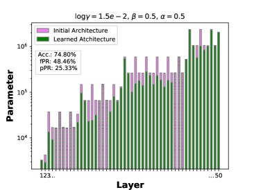
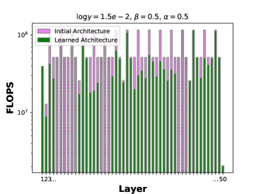
Figure 2: The number of Parameters and FLOPS in all layers of the learned architecture using our method with hyperparameters $\log\gamma={1.5}\mathrm{e}{-2},\beta=0.5,\alpha=0.5$ (green) and of the original ResNet50 architecture (violet) in logarithmic vertical scale. Layers that have been pruned completely are shaded.

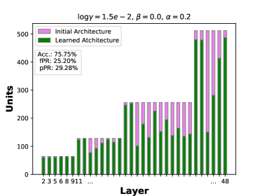
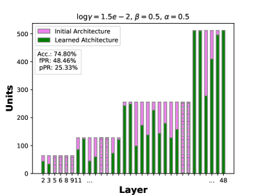
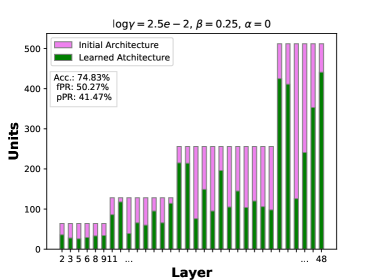
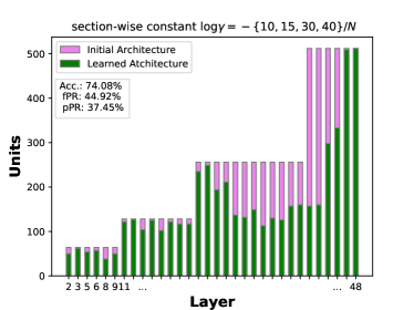
Figure 3: Top row and bottom left: The number output units of the layers that are multiplied by a $\xi$ RV using our method for different selections of hyperparameters (green) and of the original ResNet50 architecture (violet). Layers that have been pruned completely are shaded. Bottom right: The number output units of the layers of the network found using [13]-B.

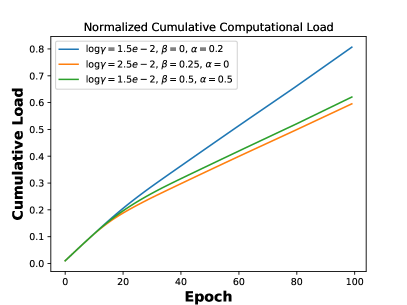
Figure 4: The normalized cumulative load of our method applied to ResNet50 and the ImageNet dataset. Training the original ResNet50 architecture for 100 epochs leads to a normalized cumulative load of 1.

6.2 CIFAR-100

We report the results of evaluating our method on the CIFAR-100 dataset using ResNet110 in Table 3. Similar computation (fPR) and parameter (pRP) pruning ratios were achieved in [16] via layer pruning, only after a tedious hand-tuned selection of the regularization parameters similar to $\log\gamma_{B}^{l}$ individually for each network block. In particular, to achieve a higher pPR [16]-B uses a $5$ times higher regularization parameter in the deeper layers of ResNet110, which hold the most parameters. The method proposed in this work does not require layer-wise hyperparameters and by choosing $\log\gamma={1}\mathrm{e}{-5},\beta=0.5,\alpha=0$, the fPR considerably improves over [16]-B while achieving a higher test accuracy. At the same time the pPR is drastically higher than the one in [16]-A for a similar accuracy.

Using our method with $\log\gamma_{F}=\log\gamma_{P}=0$ and $f_{B}=-250$ (instead of using the reparametrization (13)) emulates layer-only pruning and achieves a fPR of about $46\%$. Using the flexibility of combined layer and unit pruning and choosing $\log\gamma={3}\mathrm{e}{-3},\beta=0.5,\alpha=0.1$, our method improves the fPR to over $48\%$ and also achieves a slightly higher test accuracy. It is worth noting that the networks found with better pruning ratios have more layers than those found by the layer only pruning method of [16]; this demonstrates that the proposed method has the potential to discover a more balanced structures with better computational properties.

Method	Test Acc. [%]	Baseline [%]	Layer Left	fPR[%]	pPR[%]
$\log\gamma={1}\mathrm{e}{-5},\beta=0.5,\alpha=0$	75.20	75.50	102	28.08	22.87
$\log\gamma={3}\mathrm{e}{-3},\beta=0.5,\alpha=0.1$	74.57	75.50	82	48.49	44.55
$\log\gamma_{F}=\log\gamma_{P}=0$, $f_{B}=-250$	$74.32$	$75.50$	$60$	$46.26$	$45.05$
Layer Pruning [16]-A	$75.34$	$75.50$	$80$	$27.99$	$8.06$
Layer Pruning [16]-B	$75.05$	$75.50$	$88$	$20.06$	$19.56$

Table 3: Resulting test accuracy, the number of layers in the network, the FLOPS pruning ratio (fPR) and parameter pruning (pPR) ratio of the pruned networks found with our method and [16] applied to ResNet110 on the CIFAR-100 dataset.

6.3 CIFAR-10

We evaluate our method on CIFAR-10 with ResNet56 and ResNet110 to further show its effectiveness and ease of use. Table 4 shows the results for ResNet56. We use two different regularization levels of $\log\gamma={3}\mathrm{e}{-3}$ and $\log\gamma={8}\mathrm{e}{-3}$ as well as several choices for $\beta$ to trade-off FLOPS and parameter pruning. Again, computation or parameter pruning can be easily emphasized by varying $\beta$. Using $\log\gamma={3}\mathrm{e}{-3},\beta=1.7,\alpha=0$, our method achieves a pPR of 30%, similar to the layer pruning of [16]-A, while improving considerably the fPR at the cost of slightly reduced accuracy. Note that for $\beta=1.7$ we obtain $\log\gamma_{P}>0$ from (13). However, due to the specific values of $f_{1}^{l},f_{2}^{l},p_{1}^{l},p_{2}^{l}$ in ResNet56 and not considering any $\xi_{2}^{l}$ RV, there still exists a constant $R_{m}$ such that (26) holds and the stability results of Section 5 can be extended to this case. The choice $\log\gamma={8}\mathrm{e}{-3},\beta=1,\alpha=0$ yields a network with similar fPR but much higher pPR when compared to [16]-C. In comparison to the unit pruning of [13], a similar fPR can be achieved using $\log\gamma={8}\mathrm{e}{-3},\beta=0,\alpha=0$ or when a structure with fewer layers is preferred with $\log\gamma={3}\mathrm{e}{-3},\beta=1,a=0.8$, which yields a network with only 34 layers but more parameters. We find that unit pruning by itself provides the best result in terms of maximal parameter pruning.

Our method with the choice $\log\gamma={3}\mathrm{e}{-3},\beta=0.5,\alpha=0$ leads to the same accuracy as [30]-0.6 but improves both fPR and pPR considerably, while reducing the computational load of training by a factor of about 1.7. In comparison to the unit and layer pruning of [29], our network achieves a higher pPR at a slightly reduced test accuracy. We note that [29] retrains a pre-trained network requiring additional computational load and yields a pruned network that performs better than its baseline network in this example.

Method/Parameter	Test Acc. [%]	Bsln. Acc. [%]	Layer Left	fPR [%]	pPR [%]
$\log\gamma={3}\mathrm{e}{-3},\beta=1.7,\alpha=0$	93.40	94.26	46	48	30
$\log\gamma={3}\mathrm{e}{-3},\beta=0.5,\alpha=0$	93.38	94.26	46	47	50
$\log\gamma={3}\mathrm{e}{-3},\beta=0,\alpha=0$	93.59	94.26	50	32	51
$\log\gamma={3}\mathrm{e}{-3},\beta=1,\alpha=0.8$	93.07	94.26	40	56	55
$\log\gamma={8}\mathrm{e}{-3},\beta=1,\alpha=0$	92.53	94.26	34	67	60
$\log\gamma={8}\mathrm{e}{-3},\beta=0,\alpha=0$	92.65	94.26	42	51	67
Layer Pruning [16]-A	93.66	94.26	34	39	28
Layer Pruning [16]-C	92.64	94.26	22	63	46
Unit Pruning [13]	92.45	94.26	56	54	84
[29]	93.76	93.69	-	50	40
[30]-0.6	93.38	93.26	36	38	12
[30]-0.8	91.58	93.26	24	60	66

Table 4: Resulting test accuracy, the number of layers in the network, the FLOPS pruning ratio (fPR) and parameter pruning (pPR) ratio of the pruned networks found with our method and [13, 16, 29, 30] applied to ResNet56 on the CIFAR-10 dataset.

Table 5 summarizes the results using the ResNet110 architecture. In comparison to [30] the proposed method achieves higher test accuracies with higher pruning ratios. When compared to [16]-B, the proposed method with $\log\gamma={4}\mathrm{e}{-3},\beta=0,\alpha=0$, and hence actively favoring a network with few parameters, achieves a considerably higher pPR for a slight decrease in test accuracy.

Method/Parameter	Test Acc. [%]	Bsln. Acc. [%]	Layer Left	fPR [%]	pPR [%]
$\log\gamma={1}\mathrm{e}{-5},\beta=0.5,\alpha=0$	94.55	94.70	90	41	44
$\log\gamma={4}\mathrm{e}{-3},\beta=1,\alpha=0$	93.44	94.70	56	77	74
$\log\gamma={4}\mathrm{e}{-3},\beta=0,\alpha=0$	93.57	94.70	65	64	78
Layer Pruning [16]-A	94.25	94.70	51	54	44
Layer Pruning [16]-B	93.86	94.70	41	63	53
[30]-0.1	93.59	93.5	90	18.7	4.1
[30]-0.5	92.74	93.5	-	48.5	44.8

Table 5: Resulting test accuracy, the number of layers in the network, the FLOPS pruning ratio (fPR) and parameter pruning (pPR) ratio of the pruned networks found with our method and [16, 30] applied to ResNet110 on the CIFAR-10 dataset.

7 Conclusion

We have proposed a novel algorithm for combined unit/filter and layer pruning of DNNs that functions during training and without requiring a pre-trained network to apply. Our algorithm optimally trades-off learning accuracy and pruning levels while balancing layer vs. unit/filter pruning and computational vs. parameter complexity using only three user-selected parameters that i) control the general pruning level, ii) regulate layer vs. unit pruning and iii) trade-off computational complexity vs. the number of parameters of the network, for which the best choice may be hardware dependent. Based on Bayesian variational methods, the algorithm introduces Bernoulli $0/1$ RVs scaling the output of the unit/filters and layers of the network; the optimal network structure is then found as the solution of a stochastic optimization problem over the network weights and parameters describing the variational Bernoulli distributions. Pruning occurs during the training phase when a variational parameter converges to 0 rendering the corresponding structure permanently inactive, thus saving computations not only at the prediction but also during the training phase. We place the “flattening” hyper-prior [13] on the parameters of the Bernoulli random variables and show that the solutions of the stochastic optimization problem are deterministic networks, i.e., with Bernoulli parameters at either 0 or 1, a property that was first established in [16] for layer only pruning and extended to the case of combined unit and layer pruning in this work.

A key contribution of our approach is to define a cost function that combines the objectives of prediction accuracy and network pruning in a complexity-aware manner and the automatic selection of the hyperparameters in the flattening hyper-priors. We accomplish this by relating the corresponding regularization terms in the cost function to the expected number of FLOPS and the number of parameters of the network. In this manner, all regularization parameters, as many as three times the number of layers in the network, are expressed in terms of only three user-defined parameters, which are easy to interpret. Thus, the tedious process of tuning the regularization parameters individually is circumvented, and furthermore, the latter vary dynamically, adjusting as the network complexity and the usefulness of the substructures they control evolve during training.

We analyze the ODE system that underlies our stochastic optimization algorithm and establish in Theorem 5.1 domains of attraction around zero for the dynamics of the weights of a layer and either its Bernoulli parameter or the Bernoulli parameters of all of its units. Similarly, we establish in Theorem 5.2, domains of attraction around zero for the dynamics of the weights of a unit and either its Bernoulli parameter of the Bernoulli parameter of its layer. These results provide theoretical support for safely pruning units/filters and/or layers during training and lead to practical pruning conditions.

Our proposed algorithm is computationally efficient because of the removal of unnecessary structures during training and also because it requires only first order gradients to learn the Bernoulli parameters, adding little extra computation to standard backpropagation. We evaluate our method on the CIFAR-10/100 and ImageNet datasets using common ResNet architectures and demonstrate that our combined unit/filter and layer pruning method improves upon layer only or unit only pruning with respect to pruning ratios and test accuracy and favorably competes with combined unit/filter and layer pruning algorithms that require a pre-trained network. In summary, the proposed algorithm is capable of discovering balanced network structures with better computational/parameter complexity properties at a reduced cost and with minimal effort in tuning hyperparameters.

References

- [1] R. Girshick, “Fast r-cnn,” in International Conference on Computer Vision, pp. 1440–1448, 2015.
- [2] H. Noh, S. Hong, and B. Han, “Learning deconvolution network for semantic segmentation,” in IEEE International Conference on Computer Vision, pp. 1520–1528, 2015.
- [3] D. Silver, J. Schrittwieser, K. Simonyan, I. Antonoglou, A. Huang, A. Guez, T. Hubert, L. Baker, M. Lai, A. Bolton, Y. Chen, T. Lillicrap, F. Hui, L. Sifre, G. van den Driessche, T. Graepel, and D. Hassabis, “Mastering the game of Go without human knowledge,” Nature, vol. 550, no. 7676, pp. 354–359, 2017.
- [4] K. He, X. Zhang, S. Ren, and J. Sun, “Deep residual learning for image recognition,” in 2016 IEEE Conference on Computer Vision and Pattern Recognition (CVPR), pp. 770–778, 2016.
- [5] K. He, X. Zhang, S. Ren, and J. Sun, “Identity mappings in deep residual networks,” in European Conference on Computer Vision – ECCV 2016, pp. 630–645, Springer International Publishing, 2016.
- [6] S. Ioffe and C. Szegedy, “Batch normalization: Accelerating deep network training by reducing internal covariate shift,” in Proceedings of the 32nd International Conference on International Conference on Machine Learning - Volume 37, ICML’15, p. 448–456, JMLR.org, 2015.
- [7] S. Han, J. Pool, J. Tran, and W. J. Dally, “Learning both weights and connections for efficient neural networks,” in International Conference on Neural Information Processing Systems - Volume 1, p. 1135–1143, 2015.
- [8] D. Blalock, J. J. Gonzalez Ortiz, J. Frankle, and J. Guttag, “What is the state of neural network pruning?,” in Machine Learning and Systems, vol. 2, pp. 129–146, 2020.
- [9] H. Li, A. Kadav, I. Durdanovic, H. Samet, and H. P. Graf, “Pruning filters for efficient convnets,” arXiv preprint arXiv:1608.08710, 2016.
- [10] Y. He, G. Kang, X. Dong, Y. Fu, and Y. Yang, “Soft filter pruning for accelerating deep convolutional neural networks,” in International Joint Conference on Artificial Intelligence, p. 2234–2240, 2018.
- [11] L. Liebenwein, C. Baykal, B. Carter, D. Gifford, and D. Rus, “Lost in Pruning: The Effects of Pruning Neural Networks beyond Test Accuracy,” arXiv:2103.03014 [cs], Mar. 2021. arXiv: 2103.03014.
- [12] Y. Tang, Y. Wang, Y. Xu, D. Tao, C. Xu, C. Xu, and C. Xu, “SCOP: scientific control for reliable neural network pruning,” in Proceedings of the 34th International Conference on Neural Information Processing Systems, NIPS’20, pp. 10936–10947, Curran Associates Inc., Dec. 2020.
- [13] V. F. I. Guenter and A. Sideris, “Robust learning of parsimonious deep neural networks,” Neurocomputing, vol. 566, p. 127011, 2024.
- [14] S. Chen and Q. Zhao, “Shallowing deep networks: Layer-wise pruning based on feature representations,” IEEE Transactions on Pattern Analysis and Machine Intelligence, vol. 41, no. 12, pp. 3048–3056, 2019.
- [15] W. Wang, S. Zhao, M. Chen, J. Hu, D. Cai, and H. Liu, “DBP: Discrimination based block-level pruning for deep model acceleration,” arXiv preprint arXiv:1912.10178, 2019.
- [16] V. F. I. Guenter and A. Sideris, “Concurrent training and layer pruning of deep neural networks,” arXiv preprint arXiv:2406.04549, 2024.
- [17] J. Frankle and M. Carbin, “The lottery ticket hypothesis: Finding sparse, trainable neural networks,” in International Conference on Learning Representations, 2019.
- [18] C. Louizos, K. Ullrich, and M. Welling, “Bayesian compression for deep learning,” in Advances in Neural Information Processing Systems (I. Guyon, U. V. Luxburg, S. Bengio, H. Wallach, R. Fergus, S. Vishwanathan, and R. Garnett, eds.), vol. 30, Curran Associates, Inc., 2017.
- [19] K. Zhang and G. Liu, “Layer pruning for obtaining shallower resnets,” IEEE Signal Processing Letters, vol. 29, pp. 1172–1176, 2022.
- [20] J.-H. Luo, J. Wu, and W. Lin, “Thinet: A filter level pruning method for deep neural network compression,” in IEEE International Conference on Computer Vision, pp. 5058–5066, 2017.
- [21] Z. Huang and N. Wang, “Data-driven sparse structure selection for deep neural networks,” in Computer Vision - ECCV 2018 - 15th European Conference, Munich, Germany, September 8-14, 2018, Proceedings, Part XVI (V. Ferrari, M. Hebert, C. Sminchisescu, and Y. Weiss, eds.), vol. 11220 of Lecture Notes in Computer Science, pp. 317–334, Springer, 2018.
- [22] P. Xu, J. Cao, F. Shang, W. Sun, and P. Li, “Layer pruning via fusible residual convolutional block for deep neural networks,” arXiv preprint arXiv:2011.14356, 2020.
- [23] Z. Liu, J. Li, Z. Shen, G. Huang, S. Yan, and C. Zhang, “Learning efficient convolutional networks through network slimming,” in ICCV, 2017.
- [24] D. Molchanov, A. Ashukha, and D. Vetrov, “Variational dropout sparsifies deep neural networks,” in International Conference on Machine Learning, pp. 2498–2507, 2017.
- [25] E. Nalisnick, A. Anandkumar, and P. Smyth, “A scale mixture perspective of multiplicative noise in neural networks,” arXiv preprint arXiv:1506.03208, 2015.
- [26] E. Nalisnick, J. M. Hernandez-Lobato, and P. Smyth, “Dropout as a structured shrinkage prior,” in Proceedings of the 36th International Conference on Machine Learning (K. Chaudhuri and R. Salakhutdinov, eds.), vol. 97 of Proceedings of Machine Learning Research, pp. 4712–4722, PMLR, 09–15 Jun 2019.
- [27] N. Srivastava, G. Hinton, A. Krizhevsky, I. Sutskever, and R. Salakhutdinov, “Dropout: A simple way to prevent neural networks from overfitting,” Journal of Machine Learning Research, vol. 15, no. 56, pp. 1929–1958, 2014.
- [28] Y. Gal and Z. Ghahramani, “Dropout as a bayesian approximation: Representing model uncertainty in deep learning,” arXiv preprint arXiv:1506.02142, 2015.
- [29] W. Wang, M. Chen, S. Zhao, L. Chen, J. Hu, H. Liu, D. Cai, X. He, and W. Liu, “Accelerate cnns from three dimensions: A comprehensive pruning framework,” in Proceedings of the 38th International Conference on Machine Learning (M. Meila and T. Zhang, eds.), vol. 139 of Proceedings of Machine Learning Research, pp. 10717–10726, PMLR, 18–24 Jul 2021.
- [30] S. Lin, R. Ji, C. Yan, B. Zhang, L. Cao, Q. Ye, F. Huang, and D. S. Doermann, “Towards optimal structured cnn pruning via generative adversarial learning,” 2019 IEEE/CVF Conference on Computer Vision and Pattern Recognition (CVPR), pp. 2785–2794, 2019.
- [31] C. M. Bishop, Pattern recognition and machine learning. Information science and statistics, New York: Springer, 2006.
- [32] A. Corduneanu and C. Bishop, “Variational bayesian model selection for mixture distribution,” Artificial Intelligence and Statistics, vol. 18, pp. 27–34, 2001.
- [33] Y. Bengio, N. Léonard, and A. Courville, “Estimating or propagating gradients through stochastic neurons for conditional computation,” arXiv preprint arXiv:1308.3432, 2013.
- [34] H. Kushner and G. Yin, Stochastic Approximation and Recursive Algorithms and Applications. Stochastic Modelling and Applied Probability, Springer New York, 2003.
- [35] V. S. Borkar, Stochastic Approximation: A Dynamical Systems Viewpoint. Texts and Readings in Mathematics, Hindustan Book Agency, 2009.
- [36] C. Jin, R. Ge, P. Netrapalli, S. M. Kakade, and M. I. Jordan, “How to escape saddle points efficiently,” in Proceedings of the 34th International Conference on Machine Learning (D. Precup and Y. W. Teh, eds.), vol. 70 of Proceedings of Machine Learning Research, pp. 1724–1732, PMLR, 06–11 Aug 2017.
- [37] H. Daneshmand, J. Kohler, A. Lucchi, and T. Hofmann, “Escaping saddles with stochastic gradients,” in Proceedings of the 35th International Conference on Machine Learning (J. Dy and A. Krause, eds.), vol. 80 of Proceedings of Machine Learning Research, pp. 1155–1164, PMLR, 10–15 Jul 2018.
- [38] H. K. Khalil, Nonlinear systems; 3rd ed. Upper Saddle River, NJ: Prentice-Hall, 2002.
- [39] J. Deng, W. Dong, R. Socher, L.-J. Li, K. Li, and L. Fei-Fei, “Imagenet: A large-scale hierarchical image database,” in 2009 IEEE conference on computer vision and pattern recognition, pp. 248–255, Ieee, 2009.
- [40] A. Krizhevsky, V. Nair, and G. Hinton, “Cifar-10 (canadian institute for advanced research),” http://www.cs.toronto.edu/ kriz/cifar.html.