Analysis and Optimization of Multiple-STAR-RIS Assisted MIMO-NOMA with GSVD Precoding: An Operator-Valued Free Probability Approach

Abstract

Among the key enabling 6G techniques, multiple-input multiple-output (MIMO) and non-orthogonal multiple-access (NOMA) play an important role in enhancing the spectral efficiency of the wireless communication systems. To further extend the coverage and the capacity, the simultaneously transmitting and reflecting reconfigurable intelligent surface (STAR-RIS) has recently emerged out as a cost-effective technology. To exploit the benefit of STAR-RIS in the MIMO-NOMA systems, in this paper, we investigate the analysis and optimization of the downlink dual-user MIMO-NOMA systems assisted by multiple STAR-RISs under the generalized singular value decomposition (GSVD) precoding scheme, in which the channel is assumed to be Rician faded with the Weichselberger’s correlation structure. To analyze the asymptotic information rate of the users, we apply the operator-valued free probability theory to obtain the Cauchy transform of the generalized singular values (GSVs) of the MIMO-NOMA channel matrices, which can be used to obtain the information rate by Riemann integral. Then, considering the special case when the channels between the BS and the STAR-RISs are deterministic, we obtain the closed-form expression for the asymptotic information rates of the users. Furthermore, a projected gradient ascent method (PGAM) is proposed with the derived closed-form expression to design the STAR-RISs thereby maximizing the sum rate based on the statistical channel state information. The numerical results show the accuracy of the asymptotic expression compared to the Monte Carlo simulations and the superiority of the proposed PGAM algorithm.

I Introduction

Future communication systems are envisioned to support emerging services such as virtual reality, autonomous driving, and augmented reality, which promotes the need to further enhance the spectral efficiency and capacity of the wireless communication systems. As a key physical layer technology in 5G, multiple-input multiple-output (MIMO) plays an important role in improving the spectral efficiency and reliability of the wireless link by utilizing the spatial degree of freedom (DoF) of the transfer channels [1, 2]. However, the capacity of the MIMO system with the orthogonal access scheme is limited when there are many users/streams spatially indistinguishable [3]. Therefore, to achieve the capacity gain promised by MIMO with large number of users/streams, the non-orthogonal multiple access (NOMA) schemes have emerged to boost the system capacity [4, 5], in which the data are transferred in the same time-frequency resource, and then the data are recovered at the receiver by the successive interference cancellation (SIC) mechanism [6, 7].

There are many works on the MIMO-NOMA schemes, among which the generalized singular value decomposition (GSVD) precoding stands out due to the better communication performance and low implementation complexity, especially under the high signal-to-noise ratio (SNR) [8]. Specifically, the GSVD precoding transforms the multi-user MIMO (MU-MIMO) channel into multiple parallel multi-user single-input single-output (MU-SISO) subchannels, thereby reducing the complexity of signal processing in each subchannel [9, 10]. Therefore, the performance of the GSVD-precoded MIMO-NOMA systems is gaining increasing attention. In [11], the GSVD precoding scheme was adopted in the downlink MIMO-NOMA system to improve the sum rate and the asymptotic average rates for individual users were derived under Rayleigh channels, assuming that the number of the receiving antennas at the users are the same. Furthermore, considering the line-of-sight (LoS) components of the channels, the asymptotic performance of the GSVD-precoded MIMO-NOMA system with Rician fading was investigated in [12]. With the free probability theory, the authors first derived the Cauchy transform of the generalized singular values (GSVs) of the MIMO-NOMA channels. Then, by simplifying the channels to be Rayleigh-faded, the closed-form expressions of the average rate were derived. In addition, the authors in [8] extended the scenario to a GSVD-based MIMO-NOMA system assisted by an amplify-and-forward (AF) relay, in which the closed-form expression of the probability density function (PDF) of GSVs for two MIMO channel matrices was derived for the insightful performance evaluation.

Recently, reconfigurable intelligent surface (RIS) is regarded as a promising technology in 6G to enhance the cellular communication network since it can improve the effective channel between the transmitter and the receiver by controlling the phase and amplitude of the RIS elements [13]. However, conventional RIS can only serve users on one side of the RIS panel, otherwise the signal will be blocked. To address this issue, simultaneously transmitting and reflecting RIS (STAR-RIS) is proposed to further exploit the merit of RIS to extend the coverage and improve the channel quality [15]. Specifically, STAR-RIS extends the service coverage to the full-space by transmitting and reflecting the impinging signals simultaneously [16, 17]. The distinctive feature of the STAR-RIS enables seamless integration with the NOMA technique, i.e., the users located on both sides of the STAR-RIS can be simultaneously served by the BS with the NOMA scheme. By allocating distinct powers to different users at the BS and configuring different transmission and reflection coefficients at the STAR-RIS, the signals for the two users can be effectively distinguished. Therefore, the performance analysis of STAR-RIS assisted NOMA systems has gradually attracted attention [19, 20, 18, 21]. Specifically, when the direct links between the BS and the users are blocked by the obstacles, the authors in [18] derived the closed-form expressions of ergodic rates and high signal-to-noise ratio (SNR) slopes for the downlink transmissions towards single-antenna users, where a single STAR-RIS was deployed. Furthermore, considering spatially correlated channels towards two users, the authors in [19] derived the closed-form expressions of the outage probability for two downlink NOMA users with a STAR-RIS assisted, which illustrated the performance loss due to the channel correlations for a single-input single-output (SISO) system. In addition, considering the existence of the direct links between the BS and the users, the statistical distribution of the Nakagami-m channels and the ergodic capacity of the receiving node were obtained for a STAR-RIS assisted SISO-NOMA downlink system in [20]. With multiple antennas equipped by BS in [21], the authors analyzed the approximate analytical expressions of the ergodic rate of a STAR-RIS aided downlink NOMA system, which were maximized to design the phase-shift matrix of the STAR-RIS with the statistical channel state information (CSI).

However, to the best of our knowledge, the area of STAR-RIS assisted MIMO-NOMA system with GSVD precoding remains unexplored and needs to be analyzed to obtain insights about the impacts of the GSVD-precoding scheme on the STAR-RIS assisted system performance. In addition, the scenarios considered in the existing works on GSVD-NOMA either have the simplified Rayleigh channel assumptions [11, 8], or derive results that are not general and analytical [12]. Therefore, due to the more complicated channel configuration of STAR-RIS-assisted communications with general Rician fading, the existing performance analysis approaches cannot be applied here.

To address these issues, we focus on the analysis and optimization of the asymptotic information rate of the GSVD-precoded MIMO-NOMA systems assisted by multiple STAR-RIS, which can efficiently improve the coverage and the rank deficiency of the MIMO channels [22, 23, 24]. In addition, a general Rician channel model with Weichselberger’s correlation structure is adopted. By simplifying the system configuration, the considered system can degrade to other MIMO-NOMA systems [11, 12]. In addition, compared to [34], we further develop a linearization method for the rational matrix polynomial and address the inversion of 7x7 block matrix with non-diagonal R-transform structure. The correctness of the derived closed-form expression for the information rate is verified by the derivatives and the information rate relationships under special SNR, which is not concluded in [34].

The main contributions of this paper are summarized as follows:

• We consider a multi-STAR-RIS assisted MIMO-NOMA system, where the GSVD-precoding scheme is applied to serve two users simultaneously. In addition, a general Rician MIMO channel model with Weichselberger’s correlation structure is adopted to fit a wider range of MIMO channels. By applying the operator-valued free probability theory, we obtain the Cauchy transform of the GSVs of the MIMO-NOMA channel matrices under different antenna configurations with the help of the linearization trick for the matrix-valued rational functions.

• To obtain a deep insight into the considered system, we consider a special case by setting the channels between the BS and the STAR-RISs deterministic. Then the closed-form expressions for the asymptotic information rates of the two NOMA users are obtained via the Cauchy transform of the MIMO-NOMA channel matrices. In addition, the correctness of the derived closed-form expression for the information rate is proved by verifying derivatives and the rate relationships under special scenarios, i.e., the information rate should be 0 as the noise tends to be infinite Furthermore, based on the closed-form expressions, we propose a projected gradient ascent method (PGAM) to jointly optimize the phase shifts, the transmission and reflection coefficients of the STAR-RIS to maximize the sum rate of the two users with statistical CSI. Specifically, with the derived gradients of the sum rate, we iteratively update variables and project the updated variables onto the appropriate space to satisfy the constant-modulus constraints of STAR-RIS elements, as well as the constraints of the transmission and reflection coefficients.

• We conduct comprehensive simulations to verify the accuracy of the derived Cauchy transform and the closed-form expressions for the power normalization factor and the asymptotic information rates, as well as the effectiveness of the proposed PGAM optimization algorithm. It is shown that the derived expressions match the Monte-Carlo simulations well and the STAR-RIS can provide significant performance gains by using the proposed PAGM algorithm.

The rest of the paper is organized as follows. The system model is introduced in Section II. In Section III, we derive the Cauchy transform for the GSVs of the STAR-RIS assisted MIMO-NOMA channel and the explicit expression for the GSVD-precoding scheme. The closed-form expressions for the asymptotic information rates and the proposed PGAM algorithm are demonstrated in Section IV. The simulation results are illustrated in Section V. Finally, we conclude the main findings of the paper in Section VI.

Notations: In this paper, we denote scalars, vectors and matrices as the non-bold letters, lowercase bold letters and uppercase bold letters, respectively. $\bf{0}$ represent all-zero matrix and ${\bf{I}}_{N}$ represent the $N\times N$ identity matrix. The superscripts $(\cdot)^{*}$, $(\cdot)^{\text{T}}$ and $(\cdot)^{\dagger}$ are denoted as the conjugate, transpose and conjugate transpose operations, respectively. The notation $[\mathbf{A}]_{i,j}$ is defined as the element in the $i$-th row and $j$-th column of matrix $\mathbf{A}$. The notation $\text{diag}(\mathbf{A}_{1},\mathbf{A}_{2}\cdots,\mathbf{A}_{n})$ denotes the diagonal block matrix consisting of $\mathbf{A}_{1},\mathbf{A}_{2}\cdots,\mathbf{A}_{n}$ matrices. The operator $\text{Tr}(\cdot)$ denotes the trace of the matrix, $\mathbb{E}[\cdot]$ denotes the expectation, and $\det(\cdot)$ denotes the matrix determinant.

II System Model

II-A Signal Model

In this paper, we consider a multi-STAR-RIS assisted downlink MIMO-NOMA communication system as shown in Fig. 1, where the BS simultaneously transmits individual messages to two users located on different sides of the STAR-RIS panels . The BS is assumed to be equipped with $T$ transmit antennas and the $i$-th user is assumed to be equipped with $R_{i}$ receiving antennas for $i=1,2$. Let $\mathbf{s}_{i}\in\mathbb{C}^{T\times 1}$ denote the message sent to the $i$-th user. In the MIMO-NOMA transmission scheme, the transmit signal can be expressed as

$$\mathbf{x}=\mathbf{W}\mathbf{s}=\mathbf{W}\left(\sqrt{\kappa_{1}}\mathbf{s}_{1}+\sqrt{\kappa_{2}}\mathbf{s}_{2}\right),$$ (1)

where $\mathbf{W}$ is the precoding matrix at the BS, and $\kappa_{1}$ and $\kappa_{2}$ are the fractional power allocated to the two users, satisfying $0\leq\kappa_{i}\leq 1$ and ${\kappa_{1}}+{\kappa_{2}}=1$. In addition, the transmit signals are independent Gaussian such that $\mathbf{s}_{i}\sim CN(\mathbf{0},\mathbf{I})$ and $\mathbb{E}[\mathbf{s}_{1}\mathbf{s}_{2}^{\dagger}]=\mathbf{0}$. Assuming that the noise at the $i$-th user $\mathbf{n}_{i}$ is the additive white Gaussian noise (AWGN) with zero mean and covariance $\sigma_{0}^{2}{\bf{I}}_{R_{i}}$, the received signal at the $n$-th user can be expressed as

$$\mathbf{y}_{i}=\sqrt{\frac{{\rho_{i}}P}{t}}\mathbf{A}_{i}\left(\mathbf{R}_{0,i}+\sum_{k=1}^{K}\mathbf{R}_{k,i}\mathbf{\Theta}_{k,i}\mathbf{F}_{k}\right)\mathbf{W}\mathbf{s}+\mathbf{n}_{i},$$ (2)

where $t={\text{Tr}(\mathbf{W}\mathbf{W}^{\dagger})}$ is the power normalization factor for the precoder, $P$ is the transmit power of the BS and $\rho_{i}$ is the relative channel gain for the $i$-th user. The matrices $\mathbf{A}_{i}\in\mathbb{C}^{R_{i}\times R_{i}}$, $1\leq i\leq 2$, are the receive filter at the $i$-th user. The diagonal matrices $\mathbf{\Theta}_{k,1}=\text{diag}(\sqrt{\beta_{k,1,1}}e^{j\theta_{k,1,1}},...,\sqrt{\beta_{k,1,L_{k}}}e^{j\theta_{k,1,L_{k}}})$ and $\mathbf{\Theta}_{k,2}=\text{diag}(\sqrt{\beta_{k,2,1}}e^{j\theta_{k,2,1}},...,\sqrt{\beta_{k,2,L_{k}}}e^{j\theta_{k,2,L_{k}}})$ denote the transmitting and reflecting phase-shifting matrices of the STAR-RISs, respectively. The parameters $0\leq\sqrt{\beta_{k,i,l}}\leq 1$ and $\theta_{k,i,l}\in[0,2\pi)$ denote the fractional power and the phase shifts of the transmitting side ($i=1$) or the reflecting side ($i=2$), where $\beta_{k,1,l}+\beta_{k,2,l}=1$ for $1\leq k\leq K$ and $1\leq l\leq L_{k}$. The matrices $\mathbf{R}_{0,i}\in\mathbb{C}^{R_{i}\times T}$ denote the channels from the BS to the $i$-th user and the matrices $\mathbf{F}_{k}\in\mathbb{C}^{L_{k}\times T}$ denote the channels from the BS to the $k$-th STAR-RIS and $\mathbf{R}_{k,i}\in\mathbb{C}^{R_{i}\times L_{k}}$ denote the channel from the $k$-th STAR-RIS to the $i$-th user, where $L_{k}$ is the number of transmitting and reflecting elements in $k$-th STAR-RIS panel.

II-B Channel Model

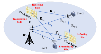
Figure 1: STAR-RIS assisted MIMO-NOMA communication system.

In this paper, to capture a general spatial correlation structure of the channels, we assume all the channels $\mathbf{F}_{k}$ and $\mathbf{R}_{k,i}$ are Rician faded with the Weichselberger’s correlation structure [25], which can be modeled as

$$\mathbf{F}_{k} =\overline{\mathbf{F}}_{k}+\widetilde{\mathbf{F}}_{k}=\overline{\mathbf{F}}_{k}+\mathbf{U}_{k}(\mathbf{M}_{k}\odot\widetilde{\mathbf{X}}_{k})\mathbf{V}_{k}^{\dagger},$$ (3)

$$\mathbf{R}_{k,i} =\overline{\mathbf{R}}_{k,i}+\widetilde{\mathbf{R}}_{k,i}=\overline{\mathbf{R}}_{k,i}+\mathbf{T}_{k,i}(\mathbf{N}_{k,i}\odot\widetilde{\mathbf{Y}}_{k,i})\mathbf{S}_{k,i}^{\dagger},$$ (4)

where $\mathbf{F}_{k}$ for $1\leq k\leq K$ and $\mathbf{R}_{k,i}$ for $1\leq i\leq 2,0\leq k\leq K$. The matrices $\overline{\mathbf{F}}_{k}$ and $\overline{\mathbf{R}}_{k,i}$ are the deterministic LoS components of the channels. The deterministic matrices $\mathbf{U}_{k}$, $\mathbf{V}_{k}$, $\mathbf{T}_{k,i}$, and $\mathbf{S}_{k,i}$ are unitary, which denote the correlation between the channel coefficients. The elements in the matrices $\mathbf{M}_{k}$ and $\mathbf{N}_{k,i}$ are nonnegative that control the variance of $\widetilde{\mathbf{F}}_{k}$ and $\widetilde{\mathbf{R}}_{k,i}$, respectively. The matrices $\widetilde{\mathbf{X}}_{k}$ and $\widetilde{\mathbf{Y}}_{k,i}$ are complex Gaussian random matrices with independent identically distributed variables with zero mean and equal variance, i.e., $[\widetilde{\mathbf{X}}_{k}]_{l,j}\sim\mathcal{CN}(0,1/T)$, $[\widetilde{\mathbf{Y}}_{0,i}]_{l,j}\sim\mathcal{CN}(0,1/R_{i})$ and $[\widetilde{\mathbf{Y}}_{k,i}]_{l,j}\sim\mathcal{CN}(0,1/L_{k})$ for $1\leq k\leq K$.

In addition, the channels $\mathbf{F}_{k}$ and $\mathbf{R}_{k,i}$ corresponding to different links are assumed to be independent. To facilitate subsequent derivations, we define the parameterized one-sided correlation matrices of $\widetilde{\mathbf{R}}_{k,i}$ as

$$\eta_{k,i}(\widetilde{\mathbf{C}}) =\mathbb{E}[\widetilde{\mathbf{R}}_{k,i}^{\dagger}\widetilde{\mathbf{C}}\widetilde{\mathbf{R}}_{k,i}]=\frac{1}{\hat{L}_{k,i}}{\mathbf{S}}_{k,i}\mathbf{\Pi}_{k,i}(\widetilde{\mathbf{C}}){\mathbf{S}}_{k,i}^{\dagger},$$ (5)

$$\widetilde{\eta}_{k,i}({\mathbf{C}}) =\mathbb{E}[\widetilde{\mathbf{R}}_{k,i}{\mathbf{C}}\widetilde{\mathbf{R}}_{k,i}^{\dagger}]=\frac{1}{\hat{L}_{k,i}}\mathbf{T}_{k,i}\widetilde{\mathbf{\Pi}}_{k,i}({\mathbf{C}})\mathbf{T}_{k,i}^{\dagger},$$ (6)

where $0\leq k\leq K$, $1\leq i\leq 2$ and $\hat{L}_{k,i}=R_{i}$ for $k=0$ and $\hat{L}_{k,i}=L_{k}$ for $k>0$. The matrices $\widetilde{\mathbf{C}}\in\mathbb{C}^{R_{i}\times R_{i}}$ and ${\mathbf{C}}\in\mathbb{C}^{\hat{L}_{k,i}\times\hat{L}_{k,i}}$ are arbitrary Hermitian matrices. The entries of the diagonal matrices $\mathbf{\Pi}_{k,i}(\widetilde{\mathbf{C}})$ and $\widetilde{\mathbf{\Pi}}_{k,i}({\mathbf{C}})$ are

$$\left[\mathbf{\Pi}_{k,i}(\widetilde{\mathbf{C}})\right]_{l,l}\! =\sum_{j=1}^{R_{i}}\left([\mathbf{N}_{k,i}]_{j,l}\right)^{2}\left[\mathbf{T}_{k,i}^{\dagger}\widetilde{\mathbf{C}}\mathbf{T}_{k,i}\right]_{j,j},1\leq l\leq\hat{L}_{k,i},$$ (7)

$$\left[\widetilde{\mathbf{\Pi}}_{k,i}({\mathbf{C}})\right]_{l,l} =\sum_{j=1}^{\hat{L}_{k,i}}\left([\mathbf{N}_{k,i}]_{l,j}\right)^{2}\left[{\mathbf{S}}_{k,i}^{\dagger}{\mathbf{C}}{\mathbf{S}}_{k,i}\right]_{j,j},1\leq l\leq R_{i}.$$ (8)

Similarly, the parameterized one-sided correlation matrices of $\widetilde{\mathbf{F}}_{k}$ are defined as

$$\zeta_{k}(\mathbf{D}_{1}) =\mathbb{E}[\widetilde{\mathbf{F}}_{k}^{\dagger}\mathbf{D}\widetilde{\mathbf{F}}_{k,i}]=\frac{1}{T}\mathbf{V}_{k}\mathbf{\Sigma}_{k}(\mathbf{D})\mathbf{V}_{k}^{\dagger},$$ (9)

$$\widetilde{\zeta}_{k}(\widetilde{\mathbf{D}}) =\mathbb{E}[\widetilde{\mathbf{F}}_{k}\widetilde{\mathbf{D}}\widetilde{\mathbf{F}}_{k}^{\dagger}]=\frac{1}{T}\mathbf{U}_{k}\widetilde{\mathbf{\Sigma}}_{k}(\widetilde{\mathbf{D}})\mathbf{U}_{k}^{\dagger},$$ (10)

where $1\leq k\leq K$ and the matrices ${\mathbf{D}}\in\mathbb{C}^{L_{k}\times L_{k}}$ and $\widetilde{\mathbf{D}}\in\mathbb{C}^{T\times T}$ are arbitrary Hermitian matrices. The diagonal matrices $\mathbf{\Sigma}_{k}$ and $\widetilde{\mathbf{\Sigma}}_{k}$ contain the diagonal entries as

$$\left[\mathbf{\Sigma}_{k}(\mathbf{D})\right]_{l,l} =\sum_{j=1}^{L_{k}}\left([\mathbf{M}_{k}]_{j,l}\right)^{2}\left[\mathbf{U}_{k}^{\dagger}\mathbf{D}\mathbf{U}_{k}\right]_{j,j},\quad 1\leq l\leq T,$$ (11)

$$\left[\widetilde{\mathbf{\Sigma}}_{k}(\widetilde{\mathbf{D}})\right]_{l,l} =\sum_{j=1}^{T}\left([\mathbf{M}_{k}]_{l,j}\right)^{2}\left[\mathbf{V}_{k}^{\dagger}\widetilde{\mathbf{D}}\mathbf{V}_{k}\right]_{j,j},\quad 1\leq l\leq L_{k}.$$ (12)

II-C Information Rate for GSVD Precoding

In this paper, the GSVD precoding and decoding scheme is applied to eliminate the interference between the MIMO-NOMA subchannels. Defining $\mathbf{H}_{i}=\left(\mathbf{R}_{0,i}+\sum_{k=1}^{K}\mathbf{R}_{k,i}\mathbf{\Theta}_{k,i}\mathbf{F}_{k}\right)$, we can obtain the GSVD precoding matrix $\mathbf{W}$ and the decoding matrices $\mathbf{A}_{i}$ for two users as $\mathbf{W}=\mathbf{V}^{-1}$ and $\mathbf{A}_{i}=\hat{\mathbf{U}}_{i}^{\dagger}$, where $\mathbf{V}$ and $\hat{\mathbf{U}}_{i}$ are obtained by applying GSVD to the channel matrices $\mathbf{H}_{1}$ and $\mathbf{H}_{2}$, which can be expressed as

$$\mathbf{H}_{i}=\hat{\mathbf{U}}_{i}\mathbf{\Sigma}_{i}\mathbf{V},$$ (13)

where $\hat{\mathbf{U}}_{i}$ is a unitary matrix and $\mathbf{V}$ is a nonsingular matrix and $\mathbf{\Sigma}_{i}$ is a rectangular diagonal matrix. With the GSVD precoding matrix $\mathbf{W}$ and the decoding matrices $\mathbf{A}_{i}$, the received signal in (2) can be repressed as

$$\mathbf{y}_{i}=\sqrt{\frac{\rho_{i}P}{t}}\mathbf{A}_{i}\mathbf{H}_{i}\mathbf{W}\mathbf{s}+\mathbf{n}_{i}=\sqrt{\frac{\rho_{i}P}{t}}\mathbf{\Sigma}_{i}\mathbf{s}+\mathbf{n}_{i}.$$ (14)

Therefore, the expressions for information rate are related to the matrix $\mathbf{\Sigma}_{i}$, which is dependent on the numbers of transmitting antennas and receiving antennas. With the statistical CSI obtained, we adopt a statistical CSI-based SIC scheme to eliminate the interference between two users [12, 26], in which the user with better average channel conditions conducts SIC, i.e., we assume $\mathbb{E}\left[\text{Tr }\left(\rho_{1}\mathbf{H}_{1}\mathbf{H}_{1}^{\dagger}\right)\right]>\mathbb{E}\left[\text{Tr }\left(\rho_{2}\mathbf{H}_{2}\mathbf{H}_{2}^{\dagger}\right)\right]$ and the SIC is performed at user 1 while user 2 treats the signal of user 1 as noise. Let $\hat{m}=\min(R_{1},R_{2})$, according to the definition of GSVD, the information rates for two users are summarized as follows:

• When $T\leq\hat{m}$: The rectangular diagonal matrix $\mathbf{\Sigma}_{i}\in\mathbb{C}^{R_{i}\times T}$ can be expressed as $\mathbf{\Sigma}_{i}=\left[\begin{array}[]{*{20}{c}}{\hat{\mathbf{\Sigma}}_{i}}\\ {\mathbf{0}_{\hat{R}_{i}\times T}}\end{array}\right]$, where $\hat{R}_{i}=R_{i}-S$, $\hat{\mathbf{\Sigma}}_{i}=\text{diag}({\sigma_{i,1},...,\sigma_{i,S}})$ and $S=\min(R_{1},T)+\min(R_{2},T)-\min(R_{1}+R_{2},T)$. Then the information rate for the users can be expressed as

  $$I_{1}= \sum_{k=1}^{S}\log\left(1+\frac{\mu_{k}}{1+\mu_{k}}\frac{P\kappa_{1}\rho_{1}}{t\sigma_{0}^{2}}\right),$$ (15)

  $$I_{2}= \sum_{k=1}^{S}\log\left(1+\frac{\kappa_{2}P}{\kappa_{1}+(1+\mu_{k})t\sigma_{0}^{2}}\right),$$ (16)

  where $\mu_{k}=\frac{\sigma_{1,k}^{2}}{\sigma_{2,k}^{2}}$.

• When $\hat{m}\leq T<R_{1}+R_{2}$: The rectangular diagonal matrix $\mathbf{\Sigma}_{i}$ can be expressed as

  $$\mathbf{\Sigma}_{1}=\left[{\begin{array}[]{*{20}{c}}{\mathbf{0}_{S\times\hat{T}_{1}}}&{\hat{\mathbf{\Sigma}}_{1}}&{\mathbf{0}_{S\times\hat{R}_{1}}}\\ {\mathbf{0}_{\hat{R}_{1}\times\hat{T}_{1}}}&{\mathbf{0}_{\hat{R}_{1}\times S}}&{\mathbf{I}_{\hat{R}_{1}}}\end{array}}\right],$$ (19)

  $$\mathbf{\Sigma}_{2}=\left[{\begin{array}[]{*{20}{c}}{\mathbf{I}_{\hat{R}_{2}}}&{\mathbf{0}_{\hat{R}_{2}\times S}}&{\mathbf{0}_{\hat{R}_{2}\times\hat{T}_{2}}}\\ {\mathbf{0}_{S\times\hat{R}_{2}}}&{\hat{\mathbf{\Sigma}}_{2}}&{\mathbf{0}_{S\times\hat{T}_{2}}}\end{array}}\right].$$ (22)

  Then the information rates for the users can be expressed as

  $$\hat{I}_{1}= I_{1}+(T-R_{1})\log\left(1+\frac{P\rho_{1}}{t\sigma_{0}^{2}}\right),$$ (23)

  $$\hat{I}_{2}= I_{2}+(T-R_{2})\log\left(1+\frac{P\rho_{2}}{t\sigma_{0}^{2}}\right),$$ (24)

  where $I_{1}$ and $I_{2}$ are given in (15) and (16).

• When $T\geq R_{1}+R_{2}$: $\mathbf{\Sigma}_{1}=\left[\mathbf{I}_{R_{1}}\mathbf{0}_{R_{1}\times(T-R_{1})}\right]$, $\mathbf{\Sigma}_{2}=\left[\mathbf{0}_{R_{2}\times(T-R_{2})}\mathbf{I}_{R_{2}}\right]$ and the information rates for the users can be expressed as

  $$\hat{I}_{1}= (T-R_{1})\log\left(1+\frac{P\rho_{1}}{t\sigma_{0}^{2}}\right),$$ (25)

  $$\hat{I}_{2}= (T-R_{2})\log\left(1+\frac{P\rho_{2}}{t\sigma_{0}^{2}}\right).$$ (26)

Based on the above analysis, we can observe that only $I_{1}$ and $I_{2}$ in (15) and (16) are related to the channel. Therefore, we only focus on the analysis for $I_{1}$ and $I_{2}$. However, it is difficult to directly obtain the expression of $I_{i}$ since the distribution of $\mu_{k}$ is unknown. Therefore, we rewrite $I_{1}$ and $I_{2}$ equivalently in term of the Cauchy transform of $\mathcal{G}_{\mu}$ as [11]

$$I_{1}= S\int_{0}^{\frac{\rho_{1}}{t\sigma_{0}^{2}}}{\left(\frac{1}{1+x}+\frac{1}{(1+x)^{2}}\mathcal{G}_{\mu}(-(x+1)^{-1})\right)\text{d}x},$$ (27)

$$I_{2}= S\int_{0}^{\frac{\rho_{2}}{t\sigma_{0}^{2}}}{\left(-\mathcal{G}_{\mu}(-(x+1))+\kappa_{1}\mathcal{G}_{\mu}(-(\kappa_{1}x+1))\right)\text{d}x},$$ (28)

where $\mathcal{G}_{\mu}(z)=\int_{0}^{\infty}\frac{1}{z-x}\mathrm{d}F_{\mu}(x)$ and $F_{\mu}$ denotes the empirical cumulative distribution function of $\mu$. According to [11], when $R_{1}>R_{2}$, the variable $\mu$ are the non-zero eigenvalues of the matrix $\mathbf{B}$ as

$$\mathbf{B}=\left\{{\begin{array}[]{*{20}{c}}{\mathbf{H}_{1}(\mathbf{H}_{2}^{\dagger}\mathbf{H}_{2})^{-1}\mathbf{H}_{1}^{\dagger},}&{T\leq R_{2}}\\ {{\mathbf{H}}_{1}(\hat{\mathbf{H}}_{2}^{\dagger}\hat{\mathbf{H}}_{2})^{-1}{\mathbf{H}_{1}^{\dagger}},}&{R_{2}<T<R_{1}+R_{2}}\end{array}}\right.$$ (31)

where $\hat{\mathbf{H}}_{2}=\left[{\begin{array}[]{*{20}{c}}{\mathbf{H}_{2}}\\ {\Delta\hat{\mathbf{I}}}\end{array}}\right]$ and $\hat{\mathbf{I}}=[\mathbf{I}_{\hat{R}_{2}}\mathbf{0}_{\hat{R}_{2}\times T}]$, in which $\Delta\to 0$ [12]. When $R_{2}>R_{1}$, $\mu$ corresponds to the eigenvalues of $\mathbf{B}$ by switching $\mathbf{H}_{1}$ and $\mathbf{H}_{2}$ in (31). Then the Cauchy transform $\mathcal{G}_{\mu}(z)$ for $R_{2}\leq R_{1}$ can be expressed as

$$\mathcal{G}_{\mu}(z)=\left\{{\begin{array}[]{*{20}{c}}{\frac{R_{1}}{S}\mathcal{G}_{\mathbf{B}}(z)-\frac{R_{1}-S}{Sz},}&{T\leq R_{2}}\\ {\frac{R_{1}}{S}\mathcal{G}_{\mathbf{B}}(z),}&{R_{2}<T<R_{1}+R_{2}}\end{array}}\right.$$ (34)

where $\mathcal{G}_{\mathbf{B}}(z)$ denotes the Cauchy transform of $\mathbf{B}$. In the next section, we will focus on the derivation of $\mathcal{G}_{\mathbf{B}}(z)$ and the expression of the normalization factor $t$, which will be used to derive the closed-form expression of the information rates of users in (27) and (28).

III Cauchy Transform and the Power Normalization Factor of the STAR-RIS Assisted MIMO-NOMA with GSVD Precoding

$$\mathbb{E}_{\mathcal{D}}\left[\mathbf{X}\right]=\left[\begin{array}[]{c:c:c:c:c:c:c}\mathbb{E}\left[\{\mathbf{X}\}_{1}^{R_{1}}\right]&&&&&&\\ \hdashline&\mathbb{E}\left[\mathbf{X}_{\widetilde{\mathbf{D}}_{1}}\right]&&&&\mathbb{E}\left[\mathbf{X}_{\widetilde{\mathbf{D}}_{3}}\right]&\\ \hdashline&&\mathbb{E}\left[\{\mathbf{X}\}_{2R_{1}+L+1}^{2R_{1}+L+T}\right]&&&&\\ \hdashline&&&\mathbb{E}[\mathbf{X}_{\widetilde{\mathbf{C}}_{1}}]&&&\\ \hdashline&&&&\mathbb{E}\left[\{\mathbf{X}\}_{2R_{1}+R_{2}+2L+T+1}^{2R_{1}+R_{2}+2L+T+R_{2}}\right]&&\\ \hdashline&\mathbb{E}\left[\mathbf{X}_{\widetilde{\mathbf{D}}_{4}}\right]&&&&\mathbb{E}\left[\mathbf{X}_{\widetilde{\mathbf{D}}_{2}}\right]&\\ \hdashline&&&&&&\mathbb{E}[\mathbf{X}_{\widetilde{\mathbf{C}}_{2}}]\end{array}\right],$$ (42)

Since the information rates $I_{1}$ and $I_{2}$ have an explicit relationship with the Cauchy transform as shown in (23)-(24), in this section we will first focus on the derivations of the Cauchy transform of $\mathbf{B}$. Then the asymptotic expression for the power normalization factor $t$ is obtained by the similar way. It should be noted that the derivation for the case $T>R_{2}$ is similar to that for $T\leq R_{2}$ by substituting $\hat{\mathbf{H}}_{2}$ into ${\mathbf{H}}_{2}$ in the derivations.

Free probability theory is a powerful tool to derive the spectral distributions of the non-commutative random variables, which are free on a non-commutative probability space [27]. Therefore, the Cauchy transform of the products of asymptotically free variables can be obtained by free multiplicative convolution in the conventional free probability theory. However, in the considered problem with $\mathbf{B}=\mathbf{H}_{1}(\mathbf{H}_{2}^{\dagger}\mathbf{H}_{2})^{-1}\mathbf{H}_{1}^{\dagger}$, both $\mathbf{H}_{1}$ and $\mathbf{H}_{2}$ are composed of random non-central matrices ($\mathbf{F}_{k}$ and $\mathbf{R}_{k,i}$) with non-trivial spatial correlations, and thus, are not free over the complex algebra in the classic free probability aspect, which makes it difficult to obtain the Cauchy transform. Therefore, in order to get the Cauchy transform, we have to find a space where $\mathbf{H}_{1}$ and $\mathbf{H}_{2}$ are asymptotically free. With this motivation, we resort to the operator-valued free probability theory and the linearization trick for the matrix-valued rational function $\mathbf{B}$, which constructs a corresponding block matrix by embedding the component matrices within $\mathbf{H}_{1}$ and $\mathbf{H}_{2}$. In this way, the constructed operator-valued variables with the linearization trick are shown to be asymptotically free in the operator-valued probability space and then the Cauchy transform of $\mathbf{B}$ can be obtained by its relation with the operator-valued Cauchy transform for the linearized block matrix. For notational simplicity, we define $\mathbf{G}_{i}=[\mathbf{I}_{R},\mathbf{R}_{1,i}\mathbf{\Theta}_{1,i},...,\mathbf{R}_{K,i}\mathbf{\Theta}_{K,i}]$ and $\mathbf{F}_{i}=[\mathbf{R}_{0,i}^{\dagger},\mathbf{F}_{1}^{\dagger},...,\mathbf{F}_{K}^{\dagger}]^{\dagger}$ for $1\leq i\leq 2$. In addition, $\overline{\mathbf{G}}_{i}=[\mathbf{I}_{R},\overline{\mathbf{R}}_{1,i}\mathbf{\Theta}_{1,i},...,\overline{\mathbf{G}}_{K,i}\mathbf{\Theta}_{K,i}]$ and $\overline{\mathbf{F}}_{i}=[\overline{\mathbf{F}}_{0,i}^{\dagger},\overline{\mathbf{F}}_{1}^{\dagger},...,\overline{\mathbf{F}}_{K}^{\dagger}]^{\dagger}$ for $1\leq i\leq 2$.

III-A Cauchy Transform $\mathcal{G}_{\mathbf{B}}(z)$

Based on (27)-(34), we need to obtain Cauchy transform $\mathcal{G}_{\mathbf{B}}(z)$ to get the information rate for two users. According to (31), the matrix $\mathbf{B}$ takes the form of a rational function of $\mathbf{H}_{1}$ and $\mathbf{H}_{2}$. Applying the linearization trick for the matrix-valued rational functions [28], we can construct the linearization matrix of $\mathbf{B}$ as

$${\mathbf{L}}=\left[{\begin{array}[]{*{20}{c}}\mathbf{0}&\mathbf{0}&\mathbf{0}&\mathbf{0}&\mathbf{0}&\mathbf{0}&\mathbf{G}_{1}\\ \mathbf{0}&\mathbf{0}&\mathbf{F}_{1}&\mathbf{0}&\mathbf{0}&\mathbf{0}&-\mathbf{I}_{R_{1}+L}\\ \mathbf{0}&\mathbf{F}_{1}^{\dagger}&\mathbf{0}&\mathbf{0}&\mathbf{0}&-\mathbf{F}_{2}^{\dagger}&\mathbf{0}\\ \mathbf{0}&\mathbf{0}&\mathbf{0}&\mathbf{0}&-\mathbf{G}_{2}^{\dagger}&\mathbf{I}_{R_{2}+L}&\mathbf{0}\\ \mathbf{0}&\mathbf{0}&\mathbf{0}&-\mathbf{G}_{2}&\mathbf{I}_{R_{2}}&\mathbf{0}&\mathbf{0}\\ \mathbf{0}&\mathbf{0}&-\mathbf{F}_{2}&\mathbf{I}_{R_{2}+L}&\mathbf{0}&\mathbf{0}&\mathbf{0}\\ \mathbf{G}_{1}^{\dagger}&-\mathbf{I}_{R_{1}+L}&\mathbf{0}&\mathbf{0}&\mathbf{0}&\mathbf{0}&\mathbf{0}\\ \end{array}}\right],$$ (50)

where $L=\sum_{k=1}^{K}L_{k}$.

Let algebra $D$ denote as the $n\times n$ block matrix and $n=3R_{1}+3R_{2}+4L+T$, then according to the operator-valued free probability theory, the Cauchy transform of $\mathbf{B}$ is related to the operator-valued Cauchy transform of $\mathbf{L}$ as

$$\mathcal{G}_{\mathbf{B}}(z)=\frac{1}{R_{1}}\mathrm{Tr}\left(\left\{\mathcal{G}_{\mathbf{L}}^{\mathcal{D}}(\mathbf{\Lambda}(z))\right\}^{(1,1)}\right),$$ (51)

where $\{\cdot\}^{(1,1)}$ denotes the upper-left $R_{1}\times R_{1}$ matrix block and the operator-valued Cauchy transform $\mathcal{G}_{\mathbf{L}}^{\mathcal{D}}(\mathbf{\Lambda}(z))$ is defined as

$$\mathcal{G}_{\mathbf{L}}^{\mathcal{D}}(\mathbf{\Lambda}(z))=\mathrm{id}\circ\mathbb{E}_{\mathcal{D}}\left[\left(\mathbf{\Lambda}(z)-\mathbf{L}\right)^{-1}\right],$$ (52)

where $\mathrm{id}$ denotes the identity operator on a Hilbert space and the diagonal matrix $\mathbf{\Lambda}(z)$ is defined as

$$\mathbf{\Lambda}(z)=\begin{bmatrix}z\mathbf{I}_{R_{1}}&\mathbf{0}_{R_{1}\times(n-R_{1})}\\ \mathbf{0}_{(n-R_{1})\times R_{1}}&\mathbf{0}_{(n-R_{1})\times(n-R_{1})}\end{bmatrix}.$$ (53)

The notation $\mathbb{E}_{\mathcal{D}}\left[\mathbf{X}\right]$ is defined as the expectation of the $n\times n$ block matrix of $\mathbf{X}$, which can be expressed as (42) at the bottom of this page, in which the notation ${\{\mathbf{A}\}^{b}_{a}}$ means extracting the submatrix of $\bf A$ with elements of the rows and columns with indices from $a$ to $b$, i.e., $\left[\{\mathbf{A}\}^{b}_{a}\right]_{i,j}=\left[\mathbf{A}\right]_{i+a-1,j+a-1}$ for $1\leq i,j\leq b-a+1$. The expectations $\mathbb{E}[\mathbf{X}_{\widetilde{\mathbf{D}}_{1}}]$, $\mathbb{E}[\mathbf{X}_{\widetilde{\mathbf{D}}_{2}}]$, $\mathbb{E}[\mathbf{X}_{\widetilde{\mathbf{C}}_{1}}]$ and $\mathbb{E}[\mathbf{X}_{\widetilde{\mathbf{C}}_{2}}]$ are defined as

$$\mathbb{E}[\mathbf{X}_{\widetilde{\mathbf{D}}_{1}}] =\text{diag}\{\mathbb{E}\left[\{\mathbf{X}\}_{R_{1}+1}^{2R_{1}}\right],\mathbb{E}\left[\{\mathbf{X}\}_{2R+1}^{2R+L_{1}}\right],$$

$$\quad\quad\quad\quad\quad\quad\cdots,\mathbb{E}\left[\{\mathbf{X}\}_{2R_{1}+\sum_{k=1}^{K-1}L_{k}+1}^{2R_{1}+\sum_{k=1}^{K}L_{k}}\right]\},$$ (54)

$$\mathbb{E}[\mathbf{X}_{\widetilde{\mathbf{D}}_{2}}] =\text{diag}\{\mathbb{E}\left[\{\mathbf{X}\}_{2R_{1}+2R_{2}+2L+T+1}^{2R_{1}+3R_{2}+2L+T}\right],\mathbb{E}\left[\{\mathbf{X}\}_{D+1}^{D+L_{1}}\right],$$

$$\quad\quad\quad\quad\quad\quad\cdots,\mathbb{E}\left[\{\mathbf{X}\}_{D+\sum_{k=1}^{K-1}L_{k}+1}^{D+\sum_{k=1}^{K}L_{k}}\right]\},$$ (55)

$$\mathbb{E}[\mathbf{X}_{\widetilde{\mathbf{C}}_{1}}] =\text{diag}\{\mathbb{E}\left[\{\mathbf{X}\}_{2R_{1}+L+T+1}^{2R_{1}+R_{2}+L+T}\right],\mathbb{E}\left[\{\mathbf{X}\}_{C_{1}+1}^{C_{1}+L_{1}}\right],$$

$$\quad\quad\quad\quad\quad\quad\cdots,\mathbb{E}\left[\{\mathbf{X}\}_{C_{1}+\sum_{k=1}^{K-1}L_{k}+1}^{C_{1}+\sum_{k=1}^{K}L_{k}}\right]\}.$$ (56)

$$\mathbb{E}[\mathbf{X}_{\widetilde{\mathbf{C}}_{2}}] =\!\text{diag}\{\mathbb{E}\left[\{\mathbf{X}\}_{2R_{1}+3R_{2}+3L+T+1}^{3R_{1}+3R_{2}+3L+T}\right],\mathbb{E}\left[\{\mathbf{X}\}_{C_{2}+1}^{C_{2}+L_{1}}\right],$$

$$\quad\quad\quad\quad\quad\quad\cdots,\mathbb{E}\left[\{\mathbf{X}\}_{C_{2}+\sum_{k=1}^{K-1}L_{k}+1}^{C_{2}+\sum_{k=1}^{K}L_{k}}\right]\},$$ (57)

$$\mathbb{E}[\mathbf{X}_{\widetilde{\mathbf{D}}_{3}}] =\!\text{diag}\{\mathbb{E}\left[\{\mathbf{X}\}_{R_{1}+1:2R_{1}}^{D-R_{2}+1:D}\right],\mathbb{E}\left[\{\mathbf{X}\}_{2R_{1}+1:2R_{1}+L_{1}}^{D+1:D+L_{1}}\right],$$

$$\quad\quad\quad\cdots,\mathbb{E}\left[\{\mathbf{X}\}_{2R_{1}+\sum_{k=1}^{K-1}L_{k}+1:2R_{1}+L}^{D+\sum_{k=1}^{K-1}L_{k}+1:D+L}\right]\},$$ (58)

$$\mathbb{E}[\mathbf{X}_{\widetilde{\mathbf{D}}_{4}}] =\!\text{diag}\{\mathbb{E}\left[\{\mathbf{X}\}_{D-R_{2}+1:D}^{R_{1}+1:2R_{1}}\right],\mathbb{E}\left[\{\mathbf{X}\}_{D+1:D+L_{1}}^{2R_{1}+1:2R_{1}+L_{1}}\right],$$

$$\quad\quad\quad\cdots,\mathbb{E}\left[\{\mathbf{X}\}_{D+\sum_{k=1}^{K-1}L_{k}+1:D+L2}^{R_{1}+\sum_{k=1}^{K-1}L_{k}+1:2R_{1}+L}\right]\},$$ (59)

where $D=2R_{1}+3R_{2}+2L+T$, $C_{1}=2R_{1}+R_{2}+L+T$ and $C_{2}=3R_{1}+3R_{2}+3L+T$. The notation ${\{\mathbf{A}\}^{a:b}_{c:d}}$ means extracting the submatrix of $\bf A$ with elements of the rows with indices from $c$ to $d$ and columns with indices from $a$ to $b$.

Consider the large-dimensional regime as

$$T\to\infty,L\to\infty,R_{i}\to\infty,L/T=\epsilon_{1},R_{i}/T=\epsilon_{2},$$ (60)

where $\epsilon_{1}$ and $\epsilon_{2}$ are constants, then based on the operator-valued free probability theory, we can obtain the Cauchy transform $\mathcal{G}_{\mathbf{B}}(z)$ in the following proposition:

Proposition 1.

The Cauchy transform of $\mathbf{B}$, with $z\in\mathbb{C}^{+}$ and (60) holding, is given by

$$\mathcal{G}_{\mathbf{B}}(z)=\frac{1}{R_{1}}\mathrm{Tr}\left[\mathcal{G}_{1}(z)\right],$$ (61)

where $\mathcal{G}_{1}(z)$ is defined as

$$\mathcal{G}_{1}(z)=\left(\widetilde{\mathbf{\Psi}}-\overline{\mathbf{G}}_{1}\left(-\widetilde{\mathbf{\Phi}}_{1,1}-\mathbf{A}_{1}^{-1}\right)\overline{\mathbf{G}}_{1}^{\dagger}\right),$$ (62)

which is obtained by solving the fixed point matrix-valued equations iteratively, shown as equations (63)-(71) at the top of the next page,

$$\mathbf{A}_{1}=\left(-\widetilde{\mathbf{\Psi}}_{1,1}-\overline{\mathbf{F}}_{1}\left(-\mathbf{\mho}-\overline{\mathbf{F}}_{2}^{\dagger}\mathbf{\Pi}^{-1}\overline{\mathbf{F}}_{2}\right)^{-1}\overline{\mathbf{F}}_{1}^{\dagger}+\widetilde{\mathbf{\Psi}}_{1,2}\left(-\widetilde{\mathbf{\Psi}}_{2,2}+\overline{\mathbf{F}}_{2}\mathbf{\mho}^{-1}\overline{\mathbf{F}}_{2}^{\dagger}-\mathbf{\Omega}^{-1}\right)^{-1}\mathbf{\Omega}^{-1}\overline{\mathbf{F}}_{1}^{\dagger}\right.$$

$$\quad\quad\quad\left.+\overline{\mathbf{F}}_{1}\mathbf{\Omega}^{-1}\left(-\widetilde{\mathbf{\Psi}}_{2,2}+\overline{\mathbf{F}}_{2}\mathbf{\mho}^{-1}\overline{\mathbf{F}}_{2}^{\dagger}\right)^{-1}\widetilde{\mathbf{\Psi}}_{2,1}\widetilde{\mathbf{\Psi}}_{1,2}\overline{\mathbf{F}}_{1}\left(-\widetilde{\mathbf{\Psi}}_{2,2}+\overline{\mathbf{F}}_{2}\mathbf{\mho}^{-1}\overline{\mathbf{F}}_{2}^{\dagger}-\mathbf{\Omega}^{-1}\right)^{-1}\widetilde{\mathbf{\Psi}}_{2,1}\right)^{-1},$$ (63)

$$\mathcal{G}_{2}(z)=\left(-\widetilde{\mathbf{\Psi}}_{1,1}-\mathbf{\Sigma}^{-1}-\overline{\mathbf{F}}_{1}\mathbf{A}_{2}\overline{\mathbf{F}}_{1}^{\dagger}+\widetilde{\mathbf{\Psi}}_{1,2}\mathbf{A}_{3}\overline{\mathbf{F}}_{1}^{\dagger}+\overline{\mathbf{F}}_{1}\mathbf{A}_{4}\widetilde{\mathbf{\Psi}}_{2,1}-\widetilde{\mathbf{\Psi}}_{1,2}\mathbf{A}_{5}\widetilde{\mathbf{\Psi}}_{2,1}\right)^{-1},$$ (64)

$$\mathcal{G}_{3}(z)=\left(-\mho-\overline{\mathbf{F}}_{1}^{\dagger}\mathbf{O}^{-1}\overline{\mathbf{F}}_{1}-\left(\overline{\mathbf{F}}_{2}^{\dagger}+\overline{\mathbf{F}}_{1}^{\dagger}\mathbf{O}^{-1}\widetilde{\mathbf{\Psi}}_{1,2}\right)\left(-\widetilde{\mathbf{\Psi}}_{2,2}-\widetilde{\mathbf{\Psi}}_{2,1}\mathbf{O}^{-1}\widetilde{\mathbf{\Psi}}_{1,2}-\mathbf{\Omega}^{-1}\right)^{-1}\left(\overline{\mathbf{F}}_{2}+\widetilde{\mathbf{\Psi}}_{2,1}\mathbf{O}^{-1}\overline{\mathbf{F}}_{1}\right)\right)^{-1},$$ (65)

$$\mathcal{G}_{4}(z)=\left(\mathbf{\Omega}-\left(-\widetilde{\mathbf{\Psi}}_{2,2}-\left(\overline{\mathbf{F}}_{2}+\widetilde{\mathbf{\Psi}}_{2,1}\mathbf{O}^{-1}\overline{\mathbf{F}}_{1}\right)\left(-\mho-\overline{\mathbf{F}}_{1}^{\dagger}\mathbf{O}^{-1}\overline{\mathbf{F}}_{1}\right)^{-1}\left(\overline{\mathbf{F}}_{2}^{\dagger}+\overline{\mathbf{F}}_{1}^{\dagger}\mathbf{O}^{-1}\widetilde{\mathbf{\Psi}}_{1,2}\right)\right)^{-1}\right)^{-1},$$ (66)

$$\mathcal{G}_{5}(z)=\!\left(\!-\mathbf{\Phi}_{2}-\mathbf{I}\!-\!\overline{\mathbf{G}}_{2}\left(\!-\widetilde{\mathbf{\Phi}}_{2}-\left(\!-\widetilde{\mathbf{\Psi}}_{2,2}-\left(\!\overline{\mathbf{F}}_{2}+\widetilde{\mathbf{\Psi}}_{2,1}\mathbf{O}^{-1}\overline{\mathbf{F}}_{1}\right)\left(\!-\mho-\!\overline{\mathbf{F}}_{1}^{\dagger}\mathbf{O}^{-1}\overline{\mathbf{F}}_{1}\right)^{-1}\left(\overline{\mathbf{F}}_{2}^{\dagger}+\!\overline{\mathbf{F}}_{1}^{\dagger}\mathbf{O}^{-1}\widetilde{\mathbf{\Psi}}_{1,2}\!\right)\!\right)^{-1}\!\right)^{-1}\overline{\mathbf{G}}_{2}^{\dagger}\!\right)^{-1},$$ (67)

$$\mathcal{G}_{6}(z)=\left(-\widetilde{\mathbf{\Psi}}_{2,2}-\left(\overline{\mathbf{F}}_{2}+\widetilde{\mathbf{\Psi}}_{2,1}\mathbf{O}^{-1}\overline{\mathbf{F}}_{1}\right)\left(-\mho-\overline{\mathbf{F}}_{1}^{\dagger}\mathbf{O}^{-1}\overline{\mathbf{F}}_{1}\right)^{-1}\left(\overline{\mathbf{F}}_{2}^{\dagger}+\overline{\mathbf{F}}_{1}^{\dagger}\mathbf{O}^{-1}\widetilde{\mathbf{\Psi}}_{1,2}\right)-\mathbf{\Omega}^{-1}\right)^{-1},$$ (68)

$$\mathcal{G}_{7}(z)=\left(\mathbf{\Sigma}-\mathbf{A}_{1}\right)^{-1},$$ (69)

$$\mathcal{G}_{8}(z)=\mathcal{G}_{2}(z)\overline{\mathbf{F}}_{1}\mathbf{A}_{2}-\mathcal{G}_{2}(z)\widetilde{\mathbf{\Psi}}_{1,2}\left(-\widetilde{\mathbf{\Psi}}_{2,2}+\overline{\mathbf{F}}_{2}\mathbf{\mho}^{-1}\overline{\mathbf{F}}_{2}^{\dagger}\right)^{-1},$$ (70)

$$\mathcal{G}_{9}(z)=\mathcal{G}_{3}(z)\left(\overline{\mathbf{F}}_{2}^{\dagger}+\overline{\mathbf{F}}_{1}^{\dagger}\mathbf{O}^{-1}\widetilde{\mathbf{\Psi}}_{1,2}\right)\left(-\widetilde{\mathbf{\Psi}}_{2,2}-\widetilde{\mathbf{\Psi}}_{2,1}\mathbf{O}^{-1}\widetilde{\mathbf{\Psi}}_{1,2}-\mathbf{\Omega}^{-1}\right)^{-1}.$$ (71)

in which the matrices $\mathbf{A}_{2}$-$\mathbf{A}_{5}$ and the matrix functions $\widetilde{\mathbf{\Psi}}$, ${\mathbf{\Omega}}$, ${\mathbf{\Pi}}$, $\mathbf{\Sigma}$, and $\mathbf{\Psi}_{i,j}$, $\widetilde{\mathbf{\Psi}}_{i,j}$, $\widetilde{\mathbf{\Phi}}_{i}$ and $\mathbf{\Phi}_{i}$ are given in Appendix A.

Proof.

The proof of Proposition 1 is given in Appendix B.

∎

With Proposition 1 and the relationship between the Cauchy transform $\mathcal{G}_{\mathbf{B}}(z)$ and the Cauchy transform $\mathcal{G}_{\mu}(z)$ in (34), we obtain the information rate for two users with (27) and (28) by the numerical integration method. For the case $R_{2}<T<R_{1}+R_{2}$, the Cauchy transforms for the two users are the same as in Proposition 1. The proof is similar to the case $T\leq R_{2}$ and therefore we omit it.

III-B Asymptotic Expression for Power Normalization Factor

According to [11], the power normalization factor for the GSVD precoder can be reformulated as

$$t=\text{Tr}\left(\mathbf{H}_{1}^{\dagger}\mathbf{H}_{1}+\mathbf{H}_{2}^{\dagger}\mathbf{H}_{2}\right)^{-1}.$$ (72)

Therefore, based on the operator-valued free probability theory and Anderson’s linearization trick for the matrix polynomials[29], we can obtain the asymptotic expression of the power normalization factor in the following proposition:

Proposition 2.

Define $\overline{\mathbf{G}}=\textup{diag}\{\overline{\mathbf{G}}_{1},\overline{\mathbf{G}}_{2}\}$ and $\overline{\mathbf{F}}=[\overline{\mathbf{F}}_{1}^{\dagger},\overline{\mathbf{F}}_{2}^{\dagger}]^{\dagger}$, with (60) holding and $z\to 0$, the asymptotic expression of the power normalization factor is given by

$$t=-\textup{Tr}(\hat{\mathcal{G}}_{1}),$$ (73)

where $\hat{\mathcal{G}}_{1}$ satisfies the following matrix-valued equations

$$\hat{\mathcal{G}}_{1}(z)=\left(\widetilde{\mathbf{\Psi}}_{\textup{t}}\!-\!\overline{\mathbf{F}}^{\dagger}\left(-\widetilde{\mathbf{\Psi}}_{\textup{t}}-\!\left(-\widetilde{\mathbf{\Phi}}_{\textup{t}}-\!\overline{\mathbf{G}}^{\dagger}\mathbf{\Phi}_{\textup{t}}^{-1}\overline{\mathbf{G}}\right)^{-1}\right)^{-1}\overline{\mathbf{F}}\right)^{-1},$$ (74)

$$\hat{\mathcal{G}}_{2}(z)=\left(-\widetilde{\mathbf{\Phi}}_{\textup{t}}-\overline{\mathbf{G}}^{\dagger}\mathbf{\Phi}_{\textup{t}}^{-1}\overline{\mathbf{G}}+\left(\widetilde{\mathbf{\Psi}}_{\textup{t}}+\overline{\mathbf{F}}\widetilde{\mathbf{\Psi}}_{\textup{t}}^{-1}\overline{\mathbf{F}}^{\dagger}\right)^{-1}\right)^{-1},$$ (75)

$$\hat{\mathcal{G}}_{3}(z)=\left(\mathbf{\Phi}_{\textup{t}}-\overline{\mathbf{G}}\left(\widetilde{\mathbf{\Phi}}_{\textup{t}}-\left(\widetilde{\mathbf{\Psi}}_{\textup{t}}+\overline{\mathbf{F}}\widetilde{\mathbf{\Psi}}_{\textup{t}}^{-1}\overline{\mathbf{F}}^{\dagger}\right)^{-1}\right)^{-1}\overline{\mathbf{G}}^{\dagger}\right)^{-1},$$ (76)

$$\hat{\mathcal{G}}_{4}(z)=\left(-\widetilde{\mathbf{\Psi}}_{\textup{t}}-\overline{\mathbf{F}}\widetilde{\mathbf{\Psi}}_{\textup{t}}^{-1}\overline{\mathbf{F}}^{\dagger}+\left(\widetilde{\mathbf{\Phi}}_{\textup{t}}+\overline{\mathbf{G}}^{\dagger}\mathbf{\Phi}_{\textup{t}}^{-1}\overline{\mathbf{G}}\right)^{-1}\right)^{-1},$$ (77)

where the matrices $\widetilde{\mathbf{\Psi}}_{\textup{t}}$, $\mathbf{\Phi}_{\textup{t}}$, $\widetilde{\mathbf{\Phi}}_{\textup{t}}$, and $\widetilde{\mathbf{\Psi}}_{\textup{t}}$ are given by

$$\quad\quad\quad\quad\widetilde{\mathbf{\Psi}}_{\textup{t}}=z\mathbf{I}-\mathbf{\Psi},$$ (78)

$$\quad\quad\quad\quad\mathbf{\Phi}_{\textup{t}}=\textup{diag}\left\{\sum_{k=1}^{K}\widetilde{\eta}_{k,1}(\hat{\mathcal{G}}_{2}),\sum_{k=1}^{K}\widetilde{\eta}_{k,2}(\hat{\mathcal{G}}_{2})\right\},$$ (79)

$$\quad\quad\quad\quad\widetilde{\mathbf{\Phi}}_{\textup{t}}=\textup{diag}\{\widetilde{\mathbf{\Phi}}_{1}(\hat{\mathcal{G}}_{3}),\widetilde{\mathbf{\Phi}}_{2}(\hat{\mathcal{G}}_{3})\},$$ (80)

$$\quad\quad\quad\quad\widetilde{\mathbf{\Psi}}_{\textup{t}}=\left(\!{\begin{array}[]{*{20}{c}}{\widetilde{\mathbf{\Psi}}_{1,1}(\hat{\mathcal{G}}_{1})}&{\widetilde{\mathbf{\Psi}}_{1,2}(\hat{\mathcal{G}}_{1})}\\ {\widetilde{\mathbf{\Psi}}_{2,1}(\hat{\mathcal{G}}_{1})}&{\widetilde{\mathbf{\Psi}}_{2,2}(\hat{\mathcal{G}}_{1})}\end{array}}\!\right),$$ (83)

$$\mathbf{\Psi}_{\textup{t}}=\mathbf{\Psi}_{1,1}(\hat{\mathcal{G}}_{4,1})+\mathbf{\Psi}_{1,2}(\hat{\mathcal{G}}_{4,2})+\mathbf{\Psi}_{2,1}(\hat{\mathcal{G}}_{4,3})+\mathbf{\Psi}_{2,2}(\hat{\mathcal{G}}_{4,4}).$$ (84)

Proof.

The proof of Proposition 2 is given in Appendix C. ∎

IV Closed-Form expressions of the Asymptotic Information Rate and the Proposed PGAM Optimization Algorithm

IV-A Closed-Form Expressions of the Asymptotic Information Rate

To obtain a deep insight into the considered multi-STAR-RISs assisted MIMO-NOMA system with GSVD-precoding, we consider a special case by setting the channels between the BS and the STAR-RISs deterministic, i.e., $\mathbf{F}_{k}=\overline{\mathbf{F}}_{k}$. With the simplified model, the matrix functions $\mathcal{G}_{1}(z)$-$\mathcal{G}_{7}(z)$ in Proposition 1 can be simplified as

$$\mathcal{G}_{1}(z)=\left(\widetilde{\mathbf{\Psi}}-\overline{\mathbf{G}}_{1}\left(-\widetilde{\mathbf{\Phi}}_{1,1}-\mathbf{A}_{1}^{-1}\right)\overline{\mathbf{G}}_{1}^{\dagger}\right),$$ (85)

$$\mathbf{A}_{1}=\left(-\widetilde{\mathbf{\Psi}}_{1,1}-\overline{\mathbf{F}}_{1}\left(-\mho-\overline{\mathbf{F}}_{2}^{\dagger}\mathbf{\Pi}^{-1}\overline{\mathbf{F}}_{2}\right)^{-1}\overline{\mathbf{F}}_{1}^{\dagger}\right)^{-1},$$ (86)

$$\mathcal{G}_{2}(z)=\left(-\widetilde{\mathbf{\Psi}}_{1,1}-\mathbf{\Sigma}^{-1}-\overline{\mathbf{F}}_{1}\mathbf{A}_{2}\overline{\mathbf{F}}_{1}^{\dagger}\right)^{-1},$$ (87)

$$\mathcal{G}_{3}(z)=\left(-\mho-\overline{\mathbf{F}}_{1}^{\dagger}\mathbf{O}^{-1}\overline{\mathbf{F}}_{1}-\overline{\mathbf{F}}_{2}^{\dagger}\mathbf{\Pi}^{-1}\overline{\mathbf{F}}_{2}\right)^{-1},$$ (88)

$$\mathcal{G}_{4}(z)=\left(\mathbf{\Omega}+\left(\widetilde{\mathbf{\Psi}}_{2,2}-\overline{\mathbf{F}}_{2}\left(\mho+\overline{\mathbf{F}}_{1}^{\dagger}\mathbf{O}^{-1}\overline{\mathbf{F}}_{1}\right)^{-1}\overline{\mathbf{F}}_{2}^{\dagger}\right)^{-1}\right)^{-1},$$ (89)

$$\mathcal{G}_{5}(z)=\left(-\mathbf{\Phi}_{2}-\mathbf{I}-\overline{\mathbf{G}}_{2}\left(-\widetilde{\mathbf{\Phi}}_{2}-\left(-\widetilde{\mathbf{\Psi}}_{2,2}\right.\right.\right.$$

$$\quad\left.\left.\left.-\overline{\mathbf{F}}_{2}\left(-\mho-\overline{\mathbf{F}}_{1}^{\dagger}\mathbf{O}^{-1}\overline{\mathbf{F}}_{1}\right)^{-1}\overline{\mathbf{F}}_{2}^{\dagger}\right)^{-1}\right)^{-1}\overline{\mathbf{G}}_{2}^{\dagger}\right)^{-1},$$ (90)

$$\mathcal{G}_{6}(z)=\left(\mathbf{\Pi}-\overline{\mathbf{F}}_{2}\left(-\mho-\overline{\mathbf{F}}_{1}^{\dagger}\mathbf{O}^{-1}\overline{\mathbf{F}}_{1}\right)^{-1}\overline{\mathbf{F}}_{2}^{\dagger}\right)^{-1},$$ (91)

$$\mathcal{G}_{7}(z)=\left(\mathbf{\Sigma}-\mathbf{A}_{1}\right)^{-1},$$ (92)

where the matrices $\widetilde{\mathbf{\Psi}}$, ${\mathbf{\Omega}}$, ${\mathbf{\Pi}}$, $\mathbf{\Sigma}$, and $\mathbf{\Psi}_{i,j}$, $\widetilde{\mathbf{\Psi}}_{i,j}$, $\widetilde{\mathbf{\Phi}}_{i}$ and ${\mathbf{\Phi}}_{i}$ are given in Proposition 1 by setting $\mathcal{G}_{8}(z)$ and $\mathcal{G}_{9}(z)$ to zero matrices. Then based on the relationship between the Cauchy transformation $\mathcal{G}_{\mathbf{B}}(z)$ and the information rate for two users with (27) and (28), we can derive the closed-form expressions of the asymptotic information rate in the following proposition:

Proposition 3.

With (60) holding and $\mathbf{F}_{k}=\overline{\mathbf{F}}_{k}$, the asymptotic information rates for the two users are given by

$$\overline{I}_{1}= \phi(-\frac{1}{1+\alpha_{1}})-\phi(-1)+R_{1}\log\left({1+\alpha_{1}}\right),$$ (93)

$$\overline{I}_{2}= \phi(-1-\alpha_{2})-(R_{1}-S)\log(1+\alpha_{2})-\phi(-1-\kappa_{1}\alpha_{2})$$

$$+(R_{1}-S)\log(1+\kappa_{1}\alpha_{2}),$$ (94)

where $\alpha_{i}=\frac{\rho_{i}}{t\sigma_{0}^{2}}$ and $\phi(z)$ is given by

$$\phi(z)=\log\det\left({\widetilde{\mathbf{\Psi}}(z)}\right)+\log\det\left({{\mathbf{\Sigma}}(z)}\right)+\log\det\left(-\mathbf{\Phi}_{2}-\mathbf{I}\right)$$

$$+\!\log\det\left(\mathbf{\Omega}\right)+\!\log\det\left({\mathbf{\Pi}}\right)+\!\log\det\left({\mathbf{O}}\right)+\!\log\det\left(\mathcal{G}_{3}(z)^{-1}\right)$$

$$+\textup{Tr}\left({\mathbf{\Phi}}_{1}\mathcal{G}_{1}(z)\right)+\textup{Tr}\left({\mathbf{\Phi}}_{2}\mathcal{G}_{5}(z)\right)+\textup{Tr}\left(\widetilde{{\mathbf{\Psi}}}_{1,1}\mathcal{G}_{2}(z)\right)$$

$$+\textup{Tr}\left(\widetilde{{\mathbf{\Psi}}}_{2,2}\mathcal{G}_{6}(z)\right),$$ (95)

where the involved matrices are given by (85)-(92) and Proposition 1 with setting $\mathbf{\Psi}_{1,2}$, $\mathbf{\Psi}_{2,1}$, $\widetilde{\mathbf{\Psi}}_{1,2}$, $\widetilde{\mathbf{\Psi}}_{2,1}$, $\mathcal{G}_{8}(z)$ and $\mathcal{G}_{9}(z)$ to zero matrices.

Proof.

The proof of Proposition 3 is given in Appendix D. ∎

IV-B Proposed PGAM Optimization Algorithm

Algorithm 1 PGAM Optimization Algorithm

1:initialize: Set the convergence criterion $\varepsilon$, $j=0$, $\beta_{k,1,l}=\beta_{k,2,l}=0.5$, and randomly generate the phase-shifting matrix $\mathbf{\Theta}^{(0)}$. Calculate $\bar{I}_{1}^{(0)}+\bar{I}_{2}^{(0)}$ based on (93) and (94).

2:repeat

3: Calculate the step size $\bm{\alpha}^{(i)}$ according to [31].

4: Calculate gradient $\bm{\delta}^{(j)}_{i}$ based on (184).

5: Update $\bm{\theta}^{(i+1)}$ based on (97) and (98).

6: Update power normalization factor $t$ based on Proposition 2.

7: $j=j+1$.

8:until $|\bar{I}_{1}^{(j)}+\bar{I}_{2}^{(j)}-\bar{I}_{1}^{(j-1)}-\bar{I}_{2}^{(j-1)}|<\varepsilon$.

9:output Optimal phase-shifting matrix $\mathbf{\Theta}$.

Based on the derived closed-form expressions of the information rate for two users, we can optimize the phase shifts and transmission and reflection coefficients of the STAR-RIS elements to maximize the sum rate of the two users. The optimization problem can be formulated as

$$\left({\textbf{P1}}\right) \max\limits_{{{{\bf{\Theta}}}}}~{}~{}\bar{I}_{1}(\mathbf{\Theta})+\bar{I}_{2}(\mathbf{\Theta})$$ (96a)

$$\mathrm{s.t.}\quad\mathbf{\Theta}_{k,i}=\text{diag}(\sqrt{\beta_{k,i,1}}e^{\theta_{k,i,1}},...,\sqrt{\beta_{k,i,L_{k}}}e^{\theta_{k,i,L_{k}}}),$$

$$\quad\quad\quad\quad\quad\quad\quad 1\leq k\leq K,1\leq i\leq 2,$$ (96b)

$$\quad\beta_{k,1,l}+\beta_{k,2,l}=1,1\leq k\leq K,1\leq l\leq L_{k},$$ (96c)

where $\mathbf{\Theta}\in\{\mathbf{\Theta}_{1,1},...,\mathbf{\Theta}_{K,2}\}$. It is noted that due to the constant-modulus constraint of phase shifts of the STAR-RIS, Problem (P1) is non-convex. To address this issue, we propose a PGAM algorithm to solve Problem (P1). Specifically, by applying gradient ascent method with the constraints for the phase shifts and transmission and reflection coefficients of the STAR-RIS taken into account, the sum rate increases monotonically iteratively.

Defining ${\bm{\theta}}_{i}={\mathbf{\Theta}}_{i}\mathbf{1}$ for $1\leq i\leq 2$, where $\mathbf{1}\in\mathbb{C}^{L\times 1}$ is an all-one vector and ${\mathbf{\Theta}}_{i}=\text{diag}\{\mathbf{\Theta}_{1,i},\mathbf{\Theta}_{2,i},...,\mathbf{\Theta}_{K,i}\}$. Then at the $(j+1)$-th iteration in the PGAM algorithm, the elements in the STAR-RIS are updated by

$$\bm{\theta}^{(j+1)}_{i}(l)=\text{P}_{\text{G}}\left({\bm{\theta}^{(j)}_{i}(l)+\bm{\alpha}^{(j)}_{i}(l)\bm{\delta}^{(j)}_{i}(l)}\right),$$ (97)

where $\bm{\alpha}_{i}^{(j)}$ is the step size at the $j$-th iteration and $\bm{\delta}^{(j)}_{i}$ is the gradient of $\bar{I}_{1}+\bar{I}_{2}$ at the $j$-th iteration, which is given by (187) in Appendix E. The notation $\mathbf{a}(l)$ means the $l$-th element of the vector $\mathbf{a}$ and the operator $\text{P}_{\text{G}}\left(\bm{\theta}_{i}(l)\right)$ guarantees the constraints for the phase shifts and transmission and reflection coefficients of the STAR-RIS, which is defined as

$$\text{P}_{\text{G}}\left(\bm{\theta}_{i}(l)\right)=\frac{\bm{\theta}_{i}(l)}{\sqrt{|\bm{\theta}_{2}(l)|^{2}+|\bm{\theta}_{1}(l)|^{2}}},$$ (98)

where the operator $|\bm{\theta}_{i}(l)|$ denotes the module of $\bm{\theta}_{i}(l)$. Therefore, based on (97) and (98), we proposed a PGAM optimization algorithm to solve Problem (P1), which is summarized in Algorithm 1.

For the complexity analysis, it can be noted that the complexity of the proposed PGAM algorithm mainly comes the calculation of the matrices in (75)-(82). Assuming that the number of iterations of the fixed point equation in (75)-(82) is $I_{in}$ and the number of iterations for the PGAM is $I_{out}$, the complexity of the PGAM algorithm is $O\left(I_{out}I_{in}\left((R_{1}+L)^{3}+(R_{2}+L)^{3}+T^{3}\right)\right)$

V Numerical Results

TABLE I: Parameter settings of system configurations

	$R_{1}$	$R_{2}$	$T$	$\rho_{1}$	$\rho_{2}$
Case 1	16	16	10	5	1
Case 2	10	10	16	5	1

In this section, the numerical simulations are conducted to verify the accuracy of the derived asymptotic expression of the information rates and the effectiveness of the proposed PGAM algorithm. In the simulation, for the Rician fading settings, the deterministic propagation components are modeled as the links between two UPAs equipped at both the transmitter and the receiver [32]. If not specified, the phase shifts of RIS elements are randomly generated between 0 and $2\pi$ and the transmission and reflection coefficients are set to $\beta_{k,1,l}=\beta_{k,2,l}=0.5$. The number of elements in STAR-RIS is 30 and the number of the STAR-RIS panels is set to $K=2$. In addition, we assume that the power allocation coefficients $\kappa_{i}$ for two users are set to $\kappa_{1}=0.1$ and $\kappa_{2}=0.9$. Statistical parameters of the channel in the simulations are generated randomly but fixed in each Monte Carlo simulation, such as the deterministic unitary matrices $\mathbf{U}_{k}$, $\mathbf{V}_{k}$, $\mathbf{T}_{k,i}$ and $\mathbf{S}_{k,i}$, as well as the variance matrices $\mathbf{M}_{k}$ and $\mathbf{N}_{k,i}$ in (3)-(4).

In addition, in the simulation, we consider the scenario where the attenuation of the direct link is significant due to the absorption of scatterers in the environment. Therefore, we set the channel gain of the direct links to be the same as that of each RIS-reflected link [33], i.e.,

$$\text{Tr}\left(\mathbf{R}_{0,i}\mathbf{R}_{0,i}^{\dagger}\right)=\text{Tr}\left(\left(\mathbf{G}_{k,i}\mathbf{\Theta}_{k,i}\mathbf{F}_{k}\right)\left(\mathbf{G}_{k,i}\mathbf{\Theta}_{k,i}\mathbf{F}_{k}\right)^{\dagger}\right),$$ (99)

for $1\leq i\leq 2$ and $1\leq k\leq K$.

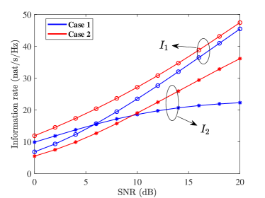
Figure 2: Information rate under different system configurations. The solid lines represent the asymptotic results with Proposition 1 and (27) and (28), and the markers represent the Monte Carlo simulation results. The specific configuration of the two cases are shown in Table I.

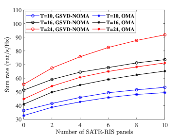
Figure 3: Sum rate versus the number of STAR-RIS panels under different SNRs. The solid lines represent the asymptotic results with Proposition 1 and (27) and (28), and the markers represent the Monte Carlo simulation results.

Figure 4: Sum rate versus the number of transmit antennas under different transmission schemes. The solid lines and the markers in red and blue represent the asymptotic results with Proposition 1, (27) and (28) and the Monte Carlo simulation results, respectively. The green lines represent the Monte Carlo simulation results for the BD scheme.

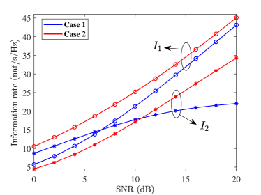
Figure 5: Information rate versus the number of STAR-RIS panels under different SNRs. The solid lines represent the asymptotic results (93) and (94), and the markers represent the Monte Carlo simulation results. The specific configuration of the two cases are shown in Table I.

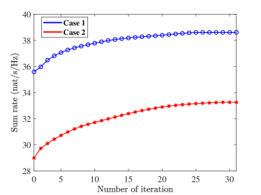
Figure 6: Sum rate versus the number of iterations under different cases. The specific configuration of the two cases are shown in Table I. The solid lines represent the asymptotic results (93) and (94) and the markers represent the Monte Carlo simulation results.

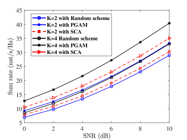
Figure 7: Sum rate versus SNR under different optimization algorithms. The solid lines and dashed lines represent the asymptotic results (93) and (94) and the markers represent the Monte Carlo simulation results.

To verify the accuracy of the derived asymptotic expressions, we plot in Fig. 2 the information rates for two users versus signal-to-noise ratio (SNR) with different system configurations. As shown in Table I, we consider two cases with different system configurations to validate the derived results with Proposition 1. The SNR is defined as $\frac{1}{\sigma_{0}^{2}}$. Each Monte Carlo simulation curve in the figure is obtained by averaging over $10^{6}$ channel realizations. In addition, for Case 2, the auxiliary variable $\Delta$ in (31) is set to $10^{-4}$ in the simulation. From Fig. 2, we observe that the analytic results match the Monte Carlo simulation results well, which shows the accuracy of the derived results of Proposition 1. In addition, in Fig. 2 of Case 1, as the SNR increases, the information rate of user 1 monotonically increases, but the information rate of user 2 tends to stabilize. This is due to the fact that with the SIC implemented at user 1, the interference of user 2 can be eliminated and hence the rate of user 1 continues to increase. However, the SIC is not deployed at user 2 and therefore, the information rate of user 2 is limited. For Case 2, the information rate for both users increases with the SNR. This is because the number of transmit antennas is larger than the number of receiving antennas in Case 2 and then there are orthogonal subchannels in the MIMO channel for transmission of user 2 in the GSVD-based precoding [11, 12]. Therefore, the information rate of user 2 is not limited by the interference of user 1 in Case 2.

To further demonstrate the merit of STAR-RIS in enhancing system performance, we depict Fig. 3 to show the relationship between the number of STAR-RIS and the sum rate $I_{1}+I_{2}$. The SNR is set to 20 dB and the number of receiving antennas is 16. In addition, we plot the sum rate under the OMA scheme to show the superiority of the GSVD-based NOMA scheme, in which we consider the time division multiple access (TDMA) protocol and the transmission scheme in [34]. It can be observed from Fig. 3 that the analytic results in Proposition 1 perfectly match the Monte Carlo simulation results for any number of STAR-RIS (including the no-RIS case, i.e., $K=0$), which further shows the generalization of our derived results. In addition, from Fig. 3, we can find that the sum rate increases with the number of STAR-RISs, but the growth of the sum rate slows down. This is due to the fact when the number of STAR-RIS is small, the reflected links are sparse, then the increment of the number of STAR-RISs riches the paths of the channel, thereby improving the sum rate effectively. However, excessive STAR-RIS panels may cause path overlap, which cannot provide much performance gain. Furthermore, compared to OMA scheme, the GSVD-based NOMA scheme can obtain a higher sum rate.

We plot Fig. 4 to further analyze the relationship between the sum rate of the GSVD precoding and the number of transmit antennas. In addition, the sum rate performance of OMA transmission scheme and the block diagonalization (BD) precoding scheme [35] are included in Fig. 4. The number of receiving antennas is set to 10 and the SNR is set to 10 dB. From Fig. 4, we can observe that the sum rate of GSVD precoding degrades when the number of transmit antennas approaches the sum of the number of receiving antennas $R_{1}+R_{2}$. This is because the power normalization factor of GSVD precoding increases significantly with the number of transmit antennas when $T\leq R_{1}+R_{2}$, which greatly decreases the power of the received signals thereby degrading the sum rate. While when $T>R_{1}+R_{2}$, the power normalization factor decreases with the increase of $T$. At the same time, the increase in the number of transmit antennas leads to more spatial gain, which results in an increase in the sum rate. Therefore, we can conclude that when $T\approx R_{1}+R_{2}$, we should adopt other NOMA schemes or OMA schemes (e.g., the BD scheme or TDMA scheme) to enhance the sum rate.

To demonstrate the accuracy of the derived closed-form expressions for information rate (93) and (94), we plot the information rate versus the SNR under different cases in Fig. 5. To apply Proposition 3, we only consider the fixed components in $\mathbf{F}_{k}$, i.e., $\widetilde{\mathbf{F}}_{k}=\mathbf{0}$. From Fig. 5, it is observed that the curves of the asymptotic results follow the Monte Carlo simulation accurately, which confirms the correctness of the derived closed-form expressions. In addition, the trends of the curves in Fig. 5 for $I_{1}$ and $I_{2}$ are the same as Fig. 2 since there are few changes in channel structure compared to Fig. 2.

To demonstrate the effectiveness of the proposed PGAM algorithm, we first depict the convergence of the PGAM algorithm (Algorithm 3) under different system cases in Fig. 6. The number of STAR-RIS panels is 2 and the number of elements for a STAR-RIS panel is 30. The SNR is fixed at 10 dB and the convergence criterion $\varepsilon$ is set to $10^{-4}$. For both cases, the sum rate increases with the number of iterations and can achieve the maximum within 25 iterations. In addition, in Fig. 6, the asymptotic results remain consistent with the simulation at any iteration, showing the compatibility of the closed-form expressions. Furthermore, the 0-th iteration in Fig. 6 implies the initial value, which is much lower than the converged sum rate, thereby indicating the effectiveness of the proposed PGAM optimization algorithm. It should be noted that the converged performance of our proposed PGAM algorithm does not depend on the initialization.

Finally, we plot Fig. 7 to demonstrate the superiority of the proposed optimization algorithm with different number of STAR-RIS panels under Case 2. The number of RIS panels is $K=2$ and $K=4$. The random scheme is the case in which the phase shifts of the STAR-RISs are randomly set and the transmission and reflection coefficients are set to $\beta_{1}=\beta_{2}=0.5$. In addition, we compare the proposed PGAM algorithm with the successive convex approximation (SCA)-based algorithm [36], in which the results obtained by each iteration are projected into the appropriate space to satisfy the constraints of the STAR-RIS. It can be clearly observed that the proposed optimization algorithm can effectively improve the sum rate in both cases. Furthermore, compared to the SCA-based algorithm, our proposed PGAM algorithm shows better performance, this is because the SCA is applied to solve the optimization problem without the constraints at each iteration and then projected the optimized phase shifts phase back to the appropriate space for the SATR-RIS. As a result, the iterations before and after cannot be matched directly. Therefore, the result of each iteration in the SCA process does not fully align with the previous iteration, which leads to the performance loss. Meanwhile, we can observe that increasing the number of STAR-RIS panels increases the optimization gain of the PGAM algorithm when the number of system antennas is fixed. This is because that more STAR-RIS panels can provide a greater optimization space, and thus the performance gain provided by the PGAM algorithm becomes higher.

VI Conclusion

In this paper, we focus on the analysis of the information rate of the MIMO-NOMA communication systems assisted by STAR-RIS, in which the GSVD precoding is applied at the BS. In addition, a general Rician channel model with Weichselberger’s correlation structure is adopted to capture the correlation between the channel coefficients. Based on the operator-valued free probability theory, we obtain the Cauchy transform of the MIMO-NOMA channel for different antenna configurations and the closed-form expression for the power normalization factor. Then, by simplifying the channel, we derive the closed-form expression of the asymptotic information rate for two users and propose a PGAM algorithm to enhance the sum rate by optimizing the STAR-RIS. Additionally, the conducted numerical results reveal the accuracy and the broadness of the derived results. Furthermore, the proposed optimization algorithm can further enhance the sum rate of the NOMA system. In addition, compared with the OMA scheme, the GSVD-based NOMA transmission scheme can obtain a higher sum rate when there is a gap between the number of transmit antennas and the sum of the number of the receiving antennas.

Appendix A The Matrix-Valued Equations in Proposition 1

The matrices $\mathbf{A}_{2}$-$\mathbf{A}_{5}$ in Proposition 1 are give by

$$\mathbf{A}_{2}=\left(-\mho-\overline{\mathbf{F}}_{2}^{\dagger}\mathbf{\Pi}^{-1}\overline{\mathbf{F}}_{2}\right)^{-1},$$ (100)

$$\mathbf{A}_{3}=\left(-\widetilde{\mathbf{\Psi}}_{2,2}+\overline{\mathbf{F}}_{2}\mathbf{\mho}^{-1}\overline{\mathbf{F}}_{2}^{\dagger}-\mathbf{\Omega}^{-1}\right)^{-1}\mathbf{\Omega}^{-1},$$ (101)

$$\mathbf{A}_{4}=\mathbf{\Omega}^{-1}\left(-\widetilde{\mathbf{\Psi}}_{2,2}+\overline{\mathbf{F}}_{2}\mathbf{\mho}^{-1}\overline{\mathbf{F}}_{2}^{\dagger}\right)^{-1},$$ (102)

$$\mathbf{A}_{5}=\left(-\widetilde{\mathbf{\Psi}}_{2,2}+\overline{\mathbf{F}}_{2}\mathbf{\mho}^{-1}\overline{\mathbf{F}}_{2}^{\dagger}-\mathbf{\Omega}^{-1}\right)^{-1}.$$ (103)

In addition, the matrix functions $\widetilde{\mathbf{\Psi}}$, ${\mathbf{\Omega}}$, ${\mathbf{\Pi}}$, $\mathbf{\Sigma}$, and $\mathbf{\Psi}_{i,j}$, $\widetilde{\mathbf{\Psi}}_{i,j}$, $\widetilde{\mathbf{\Phi}}_{i}$ and $\mathbf{\Phi}_{i}$ are respectively denoted as

$$\widetilde{\mathbf{\Psi}}=z\mathbf{I}-\mathbf{\Phi}_{1},\quad\mathbf{\Omega}=-\widetilde{\mathbf{\Phi}}_{2}-\overline{\mathbf{G}}_{2}^{\dagger}\left(-{\Phi}_{2}-\mathbf{I}\right)^{-1}\overline{\mathbf{G}}_{2},$$ (104)

$${\mathbf{\Pi}}=\widetilde{\mathbf{\Psi}}_{2,2}-\mathbf{\Omega}^{-1},\quad{\mathbf{\Sigma}}=-\widetilde{\mathbf{\Phi}}_{1}-\overline{\mathbf{G}}_{1}^{\dagger}\widetilde{\mathbf{\Psi}}^{-1}\overline{\mathbf{G}}_{1},$$ (105)

$$\mathbf{O}=-\widetilde{\mathbf{\Psi}}_{1,1}-{\mathbf{\Sigma}}^{-1},\mho=\mathbf{\Psi}_{1,1}+\mathbf{\Psi}_{2,2}-\mathbf{\Psi}_{1,2}-\mathbf{\Psi}_{2,1},$$ (106)

$$\mathbf{\Phi}_{1}=\sum_{k=1}^{K}\widetilde{\eta}_{k,1}(\mathcal{G}_{7}(z)),\quad\mathbf{\Phi}_{2}=\sum_{k=1}^{K}\widetilde{\eta}_{k,2}(\mathcal{G}_{4}(z)),$$ (107)

$$\widetilde{\mathbf{\Phi}}_{1}=\mathrm{diag}\left\{\mathbf{0},\ -\eta_{1,1}(\mathcal{G}_{1}(z)),\ \ldots,\ -\eta_{K,1}(\mathcal{G}_{1}(z))\right\},$$ (108)

$$\widetilde{\mathbf{\Phi}}_{2}=\mathrm{diag}\left\{\mathbf{0},\ -\eta_{1,2}(\mathcal{G}_{5}(z)),\ \ldots,\ -\eta_{K,2}(\mathcal{G}_{5}(z))\right\},$$ (109)

$$\widetilde{\mathbf{\Psi}}_{i,j}=\mathrm{diag}\left\{\widetilde{\zeta}_{0,i}(\mathcal{G}_{3}(z)),\widetilde{\zeta}_{1}(\mathcal{G}_{3}(z)),\ldots,\widetilde{\zeta}_{K}(\mathcal{G}_{3}(z)\right\},$$ (110)

$${\mathbf{\Psi}}_{1,1}={\zeta}_{0,1}(\mathcal{G}_{2}(z))+\sum_{k=1}^{K}{\zeta}_{K}(\mathcal{G}_{2}(z)),$$ (111)

$${\mathbf{\Psi}}_{2,2}={\zeta}_{0,1}(\mathcal{G}_{6}(z))+\sum_{k=1}^{K}{\zeta}_{K}(\mathcal{G}_{6}(z)),$$ (112)

$${\mathbf{\Psi}}_{1,2}=\sum_{k=1}^{K}{\zeta}_{k}(\mathcal{G}_{9}(z)),{\mathbf{\Psi}}_{1,2}=\sum_{k=1}^{K}{\zeta}_{k}(\mathcal{G}_{8}(z)),$$ (113)

where the matrices $\widetilde{\eta}_{k,i}$, $\eta_{k,i}$, $\widetilde{\zeta}_{k,i}$ and $\zeta_{k,i}$ are the parameterized one-sided correlation matrices of the channel as defined in (5)-(10).

Appendix B Proof of Proposition 1

According to (51), we need to calculate the operator-valued Cauchy transform $\mathcal{G}_{\mathbf{L}}^{\mathcal{D}}(\mathbf{\Lambda}(z))$ to obtain the Cauchy transform $\mathcal{G}_{\mathbf{B}}(\mathbf{\Lambda}(z))$. To explicitly calculate $\mathcal{G}_{\mathbf{L}}^{\mathcal{D}}(\mathbf{\Lambda}(z))$, the linearization matrix $\mathbf{L}$ is further expressed as

$$\mathbf{L}=\overline{\mathbf{L}}+\widetilde{\mathbf{L}},$$ (114)

where $\overline{\mathbf{L}}$ and $\widetilde{\mathbf{L}}$ contain the deterministic and the random parts of $\mathbf{L}$, respectively, and are given as follows:

$$\overline{\mathbf{L}}=\left[{\begin{array}[]{*{20}{c}}\mathbf{0}&\mathbf{0}&\mathbf{0}&\mathbf{0}&\mathbf{0}&\mathbf{0}&\overline{\mathbf{G}}_{1}\\ \mathbf{0}&\mathbf{0}&\overline{\mathbf{F}}_{1}&\mathbf{0}&\mathbf{0}&\mathbf{0}&-\mathbf{I}_{R_{1}+L}\\ \mathbf{0}&\overline{\mathbf{F}}_{1}^{\dagger}&\mathbf{0}&\mathbf{0}&\mathbf{0}&-\overline{\mathbf{F}}_{2}^{\dagger}&\mathbf{0}\\ \mathbf{0}&\mathbf{0}&\mathbf{0}&\mathbf{0}&-\overline{\mathbf{G}}_{2}^{\dagger}&\mathbf{I}_{R_{2}+L}&\mathbf{0}\\ \mathbf{0}&\mathbf{0}&\mathbf{0}&-\overline{\mathbf{G}}_{2}&\mathbf{I}_{R_{2}}&\mathbf{0}&\mathbf{0}\\ \mathbf{0}&\mathbf{0}&-\overline{\mathbf{F}}_{2}&\mathbf{I}_{R_{2}+L}&\mathbf{0}&\mathbf{0}&\mathbf{0}\\ \overline{\mathbf{G}}_{1}^{\dagger}&-\mathbf{I}_{R_{1}+L}&\mathbf{0}&\mathbf{0}&\mathbf{0}&\mathbf{0}&\mathbf{0}\\ \end{array}}\right],$$ (122)

$$\widetilde{\mathbf{L}}=\left[{\begin{array}[]{*{20}{c}}\mathbf{0}&\mathbf{0}&\mathbf{0}&\mathbf{0}&\mathbf{0}&\mathbf{0}&\widetilde{\mathbf{G}}_{1}\\ \mathbf{0}&\mathbf{0}&\widetilde{\mathbf{F}}_{1}&\mathbf{0}&\mathbf{0}&\mathbf{0}&\mathbf{0}\\ \mathbf{0}&\widetilde{\mathbf{F}}_{1}^{\dagger}&\mathbf{0}&\mathbf{0}&\mathbf{0}&-\widetilde{\mathbf{F}}_{2}^{\dagger}&\mathbf{0}\\ \mathbf{0}&\mathbf{0}&\mathbf{0}&\mathbf{0}&-\widetilde{\mathbf{G}}_{2}^{\dagger}&\mathbf{0}&\mathbf{0}\\ \mathbf{0}&\mathbf{0}&\mathbf{0}&-\mathbf{G}_{2}&\mathbf{0}&\mathbf{0}&\mathbf{0}\\ \mathbf{0}&\mathbf{0}&-\widetilde{\mathbf{F}}_{2}&\mathbf{0}&\mathbf{0}&\mathbf{0}&\mathbf{0}\\ \widetilde{\mathbf{G}}_{1}^{\dagger}&\mathbf{0}&\mathbf{0}&\mathbf{0}&\mathbf{0}&\mathbf{0}&\mathbf{0}\\ \end{array}}\right],$$ (130)

where $\overline{\mathbf{G}}_{i}$,$\overline{\mathbf{F}}_{i}$, $\widetilde{\mathbf{G}}_{i}$ and $\widetilde{\mathbf{F}}_{i}$ are defined as

$$\overline{\mathbf{G}}_{i} =[\mathbf{I}_{R},\overline{\mathbf{R}}_{1,i}\mathbf{\Theta}_{1,i},...,\overline{\mathbf{G}}_{K,i}\mathbf{\Theta}_{K,i}],$$ (131)

$$\overline{\mathbf{F}}_{i} =[\overline{\mathbf{F}}_{0,i}^{\dagger},\overline{\mathbf{F}}_{1}^{\dagger},...,\overline{\mathbf{F}}_{K}^{\dagger}]^{\dagger},$$ (132)

$$\widetilde{\mathbf{G}}_{i} =[\mathbf{0}_{R},\widetilde{\mathbf{R}}_{1,i}\mathbf{\Theta}_{1,i},...,\widetilde{\mathbf{G}}_{K,i}\mathbf{\Theta}_{K,i}],$$ (133)

$$\widetilde{\mathbf{F}}_{i} =[\widetilde{\mathbf{F}}_{0,i}^{\dagger},\widetilde{\mathbf{F}}_{1}^{\dagger},...,\widetilde{\mathbf{F}}_{K}^{\dagger}]^{\dagger}.$$ (134)

Then, with the similar steps as in [30], we can obtain that $\overline{\mathbf{L}}$ is an operator-valued semicircular variable and is free from the deterministic matrix $\widetilde{\mathbf{L}}$. Therefore, the operator-valued Cauchy transform $\mathcal{G}_{\mathbf{L}}^{\mathcal{D}}(\mathbf{\Lambda}(z))$ can be further expressed with the subordination formula [29] as

$$\mathcal{G}_{\mathbf{L}}^{\mathcal{D}}(\mathbf{\Lambda}(z)) =\mathcal{G}_{\overline{\mathbf{L}}}^{\mathcal{D}}\left(\mathbf{\Lambda}(z)-\mathcal{R}_{\widetilde{\mathbf{L}}}^{\mathcal{D}}\left(\mathcal{G}_{\mathbf{L}}^{\mathcal{D}}(\mathbf{\Lambda}(z))\right)\right)$$

$$=\mathbb{E}_{\mathcal{D}}\left[\left(\mathbf{\Lambda}(z)-\mathcal{R}_{\widetilde{\mathbf{L}}}^{\mathcal{D}}\left(\mathcal{G}_{\mathbf{L}}^{\mathcal{D}}(\mathbf{\Lambda}(z))\right)-\overline{\mathbf{L}}\right)^{-1}\right],$$ (135)

where $\mathcal{R}_{\widetilde{\mathbf{L}}}^{\mathcal{D}}\left(\cdot\right)$ denotes the operator-valued $R$-transform of $\mathbf{L}$ over $\mathcal{D}$. Then we need to calculate the operator-valued $R$-transform $\mathcal{R}_{\widetilde{\mathbf{L}}}^{\mathcal{D}}\left(\mathcal{G}_{\mathbf{L}}^{\mathcal{D}}(\mathbf{\Lambda}(z))\right)$. According to [30], given a matrix $\mathbf{K}\in\mathbb{C}^{n\times n}$, the operator-valued $R$-transform $\mathcal{R}_{\widetilde{\mathbf{L}}}^{\mathcal{D}}\left(\mathcal{G}_{\mathbf{L}}^{\mathcal{D}}(\mathbf{\Lambda}(z))\right)$ can be expressed as

$$\mathcal{R}_{\widetilde{\mathbf{L}}}^{\mathcal{D}}(\mathbf{K}) =\mathbb{E}_{\mathcal{D}}\left[\widetilde{\mathbf{L}}\mathbf{K}\widetilde{\mathbf{L}}\right]$$

$$=\left[\begin{array}[]{c:c:c:c:c:c:c}\mathbf{\Phi}_{1}&&&&&&\\ \hdashline&-\widetilde{\bm{\Psi}}_{1,1}&&&&-\widetilde{\bm{\Psi}}_{1,2}&\\ \hdashline&&{\mathbf{\mho}}&&&&\\ \hdashline&&&\widetilde{\bm{\Phi}}_{2}&&&\\ \hdashline&&&&{\bm{\Phi}}_{1}&&\\ \hdashline&-\widetilde{\bm{\Psi}}_{2,1}&&&&-\widetilde{\bm{\Psi}}_{2,2}&\\ \hdashline&&&&&&\mathbf{\Phi}_{2}\end{array}\right],$$ (143)

where the matrix functions $\widetilde{\mathbf{\Psi}}$, $\mathbf{\Psi}_{i,j}$, $\widetilde{\mathbf{\Psi}}_{i,j}$, $\widetilde{\mathbf{\Phi}}_{i}$ and $\mathbf{\Phi}_{i}$ are shown as (104)-(113) in Appendix A and the matrix $\mathbf{K}$ has the same structure as $\mathbb{E}_{\mathcal{D}}\left[\mathbf{X}\right]$ in (42).

Therefore, by replacing $\mathbf{K}$ in (143) with $\mathcal{G}_{\mathbf{L}}^{\mathcal{D}}(\mathbf{\Lambda}(z))$, and substituting $\overline{\mathbf{L}}$ and $\mathcal{R}_{\widetilde{\mathbf{L}}}^{\mathcal{D}}\left(\mathcal{G}_{\mathbf{L}}^{\mathcal{D}}(\mathbf{\Lambda}(z))\right)$ into (135), respectively, we obtain $\mathcal{G}_{\mathbf{L}}^{\mathcal{D}}(\mathbf{\Lambda}(z))$ as

$$\mathcal{G}_{\mathbf{L}}^{\mathcal{D}}(\mathbf{\Lambda}(z))$$ (144)

$$=\left[\begin{array}[]{c:c:c:c:c:c:c}z\mathbf{I}-\mathbf{\Phi}_{1}&&&&&&-\overline{\mathbf{G}}_{1}\\ \hdashline&-\widetilde{\bm{\Psi}}_{1,1}&-\overline{\mathbf{F}}_{1}&&&-\widetilde{\bm{\Psi}}_{1,2}&\mathbf{I}\\ \hdashline&-\overline{\mathbf{F}}_{1}^{\dagger}&{\mathbf{\mho}}&&&-\overline{\mathbf{F}}_{2}^{\dagger}&\\ \hdashline&&&\widetilde{\bm{\Phi}}_{2}&\overline{\mathbf{G}}_{2}^{\dagger}&-\mathbf{I}&\\ \hdashline&&&\overline{\mathbf{G}}_{2}&-{\bm{\Phi}}_{1}-\mathbf{I}&&\\ \hdashline&\widetilde{\bm{\Psi}}_{2,1}&\overline{\mathbf{F}}_{2}&-\mathbf{I}&&-\widetilde{\bm{\Psi}}_{2,2}&\\ \hdashline-\overline{\mathbf{G}}_{1}^{\dagger}&\mathbf{I}&&&&&-\mathbf{\Phi}_{2}\end{array}\right]^{-1}.$$ (152)

Then by continuously applying the block matrix inversion identity to (152), we can obtain the expression of the operator-valued Cauchy transform $\mathcal{G}_{\mathbf{L}}^{\mathcal{D}}(\mathbf{\Lambda}(z))$ and then conclude the Cauchy transform $\mathcal{G}_{\mathbf{B}}(\mathbf{\Lambda}(z))$ with $\mathcal{G}_{\mathbf{B}}(z)=\frac{1}{R_{1}}\mathrm{Tr}\left(\left\{\mathcal{G}_{\mathbf{L}}^{\mathcal{D}}(\mathbf{\Lambda}(z))\right\}^{(1,1)}\right)$, which are finally summarized in Proposition 1.

Appendix C Proof of Proposition 2

The power normalization factor for the GSVD precoder can be further reformulated as

$$t\mathop{=}\limits^{z\to 0}-\text{Tr}\left(z\mathbf{I}-\mathbf{H}_{1}^{\dagger}\mathbf{H}_{1}-\mathbf{H}_{2}^{\dagger}\mathbf{H}_{2}\right),$$ (153)

which is equal to the Cauchy transform of $\mathbf{B}_{\textup{t}}=\mathbf{H}_{1}^{\dagger}\mathbf{H}_{1}+\mathbf{H}_{2}^{\dagger}\mathbf{H}_{2}$. Therefore, we aim to obtain the Cauchy transform of $\mathbf{B}_{\textup{t}}$.

Define ${\mathbf{G}}=\textup{diag}\{{\mathbf{G}}_{1},{\mathbf{G}}_{2}\}$ and ${\mathbf{F}}=[{\mathbf{F}}_{1}^{\dagger},{\mathbf{F}}_{2}^{\dagger}]^{\dagger}$, the matrix $\mathbf{B}_{\textup{t}}$ can be expressed as $\mathbf{B}_{\textup{t}}={\mathbf{F}}^{\dagger}{\mathbf{G}}^{\dagger}{\mathbf{G}}{\mathbf{F}}$. Then following the similar method of Section III-A, we first construct the linearized matrix $\mathbf{L}_{\textup{t}}$ as

$$\mathbf{L}_{\textup{t}}=\left[\begin{array}[]{cccc}\mathbf{0}&\mathbf{0}&\mathbf{0}&\mathbf{F}^{\dagger}\\ \mathbf{0}&\mathbf{0}&\mathbf{G}^{\dagger}&-\mathbf{I}\\ \mathbf{0}&\mathbf{G}&-\mathbf{I}&\mathbf{0}\\ \mathbf{F}&-\mathbf{I}&\mathbf{0}&\mathbf{0}\end{array}\right].$$ (158)

Then substituting $\bf{G}$ and $\bf{F}$ into [30, Prop. 2] and following the same steps, we can obtain the Cauchy transform of $\mathbf{B}_{\textup{t}}$. The detailed proof is an application of Proposition 2 in [30, Prop. 2] and therefore, is omitted here. Finally, with Cauchy transform of $\mathbf{B}_{\textup{t}}$ and $z\to 0$, we can obtain Proposition 2.

Appendix D Derivation of $\overline{I}_{1}$ and $\overline{I}_{2}$

Based on (27) and (28), by differentiating $I_{1}$ and $I_{2}$ with respect to $\alpha_{1}$ and $\alpha_{2}$, we have

$$\frac{\partial I_{1}}{\partial\alpha_{1}} =\frac{S}{1+\alpha_{1}}+\frac{S}{(1+\alpha_{1})^{2}}\mathcal{G}_{\mu}(-(1+\alpha_{1})^{-1}),$$ (159)

$$\frac{\partial I_{1}}{\partial\alpha_{2}} =-S\mathcal{G}_{\mu}(-(1+\alpha_{2}))+S\mathcal{G}_{\mu}(-(1+\kappa_{1}\alpha_{2})),$$ (160)

where $\alpha_{1}$ and $\alpha_{2}$ are defined in Proposition 3. Then to prove the correctness of Proposition 3, we only need to prove that $\frac{\partial I_{1}}{\partial\alpha_{1}}=\frac{\partial\overline{I}_{1}}{\partial\alpha_{1}}$ and $\frac{\partial\overline{I}_{2}}{\partial\alpha_{2}}=\frac{\partial\overline{I}_{2}}{\partial\alpha_{2}}$ hold with the given expression in Proposition 3 and as $\sigma_{0}^{2}$ approaches infinity, $\overline{I}_{1}$ and $\overline{I}_{2}$ are equal to 0.

Therefore, the partial derivative of $\overline{I}_{1}$ with respect to $\alpha_{1}$ can be expressed as

$$\frac{\partial\overline{I}_{1}(\alpha_{1})}{\partial\alpha_{1}}=\frac{\partial\phi(\frac{-1}{1+\alpha_{1}})}{\partial\alpha_{1}}+\frac{R_{1}}{1+\alpha_{1}}$$

$$=\!\frac{\partial\!\log\det\left({\widetilde{\mathbf{\Psi}}(\lambda_{1})}\right)}{\partial\alpha_{1}}\!+\!\!\frac{\partial\!\log\det\left({{\mathbf{\Sigma}}(\lambda_{1})}\right)}{\partial\alpha_{1}}\!+\!\!\frac{\partial\!\log\det\left(-\mathbf{\Phi}_{2}\!-\!\mathbf{I}\right)}{\partial\alpha_{1}}$$

$$+\frac{\partial\log\det\left(\mathbf{\Omega}\right)}{\partial\alpha_{1}}+\frac{\partial\log\det\left({\mathbf{\Pi}}\right)}{\partial\alpha_{1}}+\frac{\partial\log\det\left(\mathcal{G}_{3}(\lambda_{1})^{-1}\right)}{\partial\alpha_{1}}$$

$$+\frac{\partial\log\det\left({\mathbf{O}}\right)}{\partial\alpha_{1}}+\frac{\partial\textup{Tr}\left({\mathbf{\Phi}}_{1}\mathcal{G}_{1}(\lambda_{1})\right)}{\partial\alpha_{1}}+\frac{\partial\textup{Tr}\left({\mathbf{\Phi}}_{2}\mathcal{G}_{5}(\lambda_{1})\right)}{\partial\alpha_{1}}$$

$$+\frac{\partial\textup{Tr}\left(\widetilde{{\mathbf{\Psi}}}_{1,1}\mathcal{G}_{2}(\lambda_{1})\right)}{\partial\alpha_{1}}+\frac{\partial\textup{Tr}\left(\widetilde{{\mathbf{\Psi}}}_{2,2}\mathcal{G}_{6}(\lambda_{1})\right)}{\partial\alpha_{1}}+\frac{R_{1}}{1+\alpha_{1}},$$ (161)

where $\lambda_{1}=\frac{-1}{1+\alpha_{1}}$. For a matrix function $\mathbf{K}(z)$, we have

$$\frac{\partial}{\partial z}\log\det\mathbf{K}(z) =\mathrm{Tr}\left(\mathbf{K}(z)^{-1}\frac{\partial\mathbf{K}(z)}{\partial z}\right),$$ (162)

$$\mathrm{Tr}\left(\frac{\partial\mathbf{K}(z)^{-1}}{\partial z}\right) =-\mathrm{Tr}\left(\mathbf{K}(z)^{-1}\frac{\partial\mathbf{K}(z)}{dz}\mathbf{K}(z)^{-1}\right).$$ (163)

Then we can obtain

$$\frac{\partial\log\det\left({\widetilde{\mathbf{\Psi}}(\lambda_{1})}\right)}{\partial\alpha_{1}}=\text{Tr}\left(\widetilde{\mathbf{\Psi}}(\lambda_{1})^{-1}\frac{\partial{\widetilde{\mathbf{\Psi}}(\lambda_{1})}}{\partial\alpha_{1}}\right),$$ (164)

$$\frac{\partial\log\det\left({{\mathbf{\Sigma}}(\lambda_{1})}\right)}{\partial\alpha_{1}}=\text{Tr}\left({\mathbf{\Sigma}}(\lambda_{1})^{-1}\frac{\partial{{\mathbf{\Sigma}}(\lambda_{1})}}{\partial\alpha_{1}}\right),$$ (165)

$$\frac{\partial\log\det\left(-\mathbf{\Phi}_{2}-\mathbf{I}\right)}{\partial\alpha_{1}}=\text{Tr}\left(\left(-\mathbf{\Phi}_{2}-\mathbf{I}\right)^{-1}\frac{\partial\left(-\mathbf{\Phi}_{2}-\mathbf{I}\right)}{\partial\alpha_{1}}\right),$$ (166)

$$\frac{\partial\log\det\left(\mathbf{\Omega}\right)}{\partial\alpha_{1}}=\text{Tr}\left(\mathbf{\Omega}^{-1}\frac{\partial\mathbf{\Omega}}{\partial\alpha_{1}}\right),$$ (167)

$$\frac{\partial\log\det\left({\mathbf{\Pi}}\right)}{\partial\alpha_{1}}=\text{Tr}\left({\mathbf{\Pi}}^{-1}\frac{\partial{\mathbf{\Pi}}}{\partial\alpha_{1}}\right),$$ (168)

$$\frac{\partial\log\det\left({\mathbf{O}}\right)}{\partial\alpha_{1}}=\text{Tr}\left({\mathbf{O}}^{-1}\frac{\partial{\mathbf{O}}}{\partial\alpha_{1}}\right),$$ (169)

$$\frac{\partial\log\det\left(\mathcal{G}_{3}(\lambda_{1})^{-1}\right)}{\partial\alpha_{1}}=\text{Tr}\left(\mathcal{G}_{3}(\lambda_{1})\frac{\partial\mathcal{G}_{3}(\lambda_{1})^{-1}}{\partial\alpha_{1}}\right).$$ (170)

In addition, according to Lemma 1 in [34] about the parameterized one-sided correlation matrices in (5) to (10), we can obtain

$$\frac{\partial\textup{Tr}\left({\mathbf{\Phi}}_{1}\mathcal{G}_{1}(\lambda_{1})\right)}{\partial\alpha_{1}}=\textup{Tr}\left(\mathcal{G}_{1}(\lambda_{1})\frac{\partial{\mathbf{\Phi}}_{1}}{\partial\alpha_{1}}\right)+\textup{Tr}\left({\mathbf{\Phi}}_{1}\frac{\partial\mathcal{G}_{1}(\lambda_{1})}{\partial\alpha_{1}}\right)$$

$$=\textup{Tr}\left(\mathcal{G}_{1}(\lambda_{1})\frac{\partial\left(\lambda_{1}\mathbf{I}-\widetilde{\mathbf{\Psi}}\right)}{\partial\alpha_{1}}\right)+\textup{Tr}\left(\mathcal{G}_{7}(\lambda_{1})\frac{\partial\widetilde{\mathbf{\Phi}}_{1,1}}{\partial\alpha_{1}}\right)$$

$$=-\lambda_{1}^{2}-\textup{Tr}\left(\mathcal{G}_{1}(\lambda_{1})\frac{\partial\widetilde{{\mathbf{\Psi}}}}{\partial\alpha_{1}}\right)+\textup{Tr}\left(\mathcal{G}_{7}(\lambda_{1})\frac{\partial\widetilde{\mathbf{\Phi}}_{1,1}}{\partial\alpha_{1}}\right).$$ (171)

Applying the matrix inversion lemma to $\mathcal{G}_{1}(\lambda_{1})$ and (163), we can obtain

$$\textup{Tr}\left(\mathcal{G}_{1}(\lambda_{1})\frac{\partial\widetilde{{\mathbf{\Psi}}}}{\partial\alpha_{1}}\right)$$

$$=\textup{Tr}\left(\left(\widetilde{{\mathbf{\Psi}}}^{-1}+\widetilde{{\mathbf{\Psi}}}^{-1}\overline{\mathbf{G}}_{1}\mathcal{G}_{7}(\lambda_{1})\overline{\mathbf{G}}_{1}^{\dagger}\widetilde{{\mathbf{\Psi}}}^{-1}\right)\frac{\partial\widetilde{{\mathbf{\Psi}}}}{\partial\alpha_{1}}\right)$$

$$=\text{Tr}\left(\widetilde{\mathbf{\Psi}}^{-1}\frac{\partial{\widetilde{\mathbf{\Psi}}}}{\partial\alpha_{1}}\right)-\textup{Tr}\left(\mathcal{G}_{7}(\lambda_{1})\overline{\mathbf{G}}_{1}^{\dagger}\frac{\partial\widetilde{{\mathbf{\Psi}}}^{-1}}{\partial\alpha_{1}}\overline{\mathbf{G}}_{1}\right).$$ (172)

Combining (171) and (172) and applying the matrix inversion lemma to $\mathcal{G}_{7}(\lambda_{1})$, we can rewrite $\frac{\partial\textup{Tr}\left({\mathbf{\Phi}}_{1}\mathcal{G}_{1}(\lambda_{1})\right)}{\partial\alpha_{1}}$ as

$$\frac{\partial\textup{Tr}\left({\mathbf{\Phi}}_{1}\mathcal{G}_{1}(\lambda_{1})\right)}{\partial\alpha_{1}}= -\lambda_{1}^{2}-\text{Tr}\left(\widetilde{\mathbf{\Psi}}^{-1}\frac{\partial{\widetilde{\mathbf{\Psi}}}}{\partial\alpha_{1}}\right)-\text{Tr}\left({\mathbf{\Sigma}}^{-1}\frac{\partial{{\mathbf{\Sigma}}}}{\partial\alpha_{1}}\right)$$

$$+\textup{Tr}\left(\mathcal{G}_{2}\frac{\partial{{\mathbf{\Sigma}}}^{-1}}{\partial\alpha_{1}}\right).$$ (173)

Similarly, we can express $\frac{\partial\textup{Tr}\left({\mathbf{\Phi}}_{2}\mathcal{G}_{5}(\lambda_{1})\right)}{\partial\alpha_{1}}$ as

$$\frac{\partial\textup{Tr}\left({\mathbf{\Phi}}_{2}\mathcal{G}_{5}(\lambda_{1})\right)}{\partial\alpha_{1}}=\textup{Tr}\left(\mathcal{G}_{5}(\lambda_{1})\frac{\partial{\mathbf{\Phi}}_{2}}{\partial\alpha_{1}}\right)+\textup{Tr}\left({\mathbf{\Phi}}_{2}\frac{\partial\mathcal{G}_{5}(\lambda_{1})}{\partial\alpha_{1}}\right)$$

$$=\textup{Tr}\left(\mathcal{G}_{5}(\lambda_{1})\frac{\partial{\mathbf{\Phi}}_{2}}{\partial\alpha_{1}}\right)+\textup{Tr}\left(\mathcal{G}_{4}(\lambda_{1})\frac{\partial\widetilde{{\mathbf{\Phi}}}_{2}}{\partial\alpha_{1}}\right).$$ (174)

With the matrix inversion lemma applied to $\mathcal{G}_{5}(\lambda_{1})$, we can obtain

$$\textup{Tr}\left(\mathcal{G}_{5}(\lambda_{1})\frac{\partial{\mathbf{\Phi}}_{2}}{\partial\alpha_{1}}\right)=-\textup{Tr}\left(\left(\left(-\mathbf{\Phi}_{2}-\mathbf{I}\right)^{-1}\right.\right.$$

$$\left.\left.+\left(-\mathbf{\Phi}_{2}-\mathbf{I}\right)^{-1}\overline{\mathbf{G}}_{2}\mathcal{G}_{4}\overline{\mathbf{G}}_{2}^{\dagger}\left(-\mathbf{\Phi}_{2}-\mathbf{I}\right)^{-1}\right)\frac{\partial\left(-{\mathbf{\Phi}}_{2}-\mathbf{I}\right)}{\partial\alpha_{1}}\right)$$

$$=-\textup{Tr}\left(\left(-\mathbf{\Phi}_{2}-\mathbf{I}\right)^{-1}\frac{\partial\left(-{\mathbf{\Phi}}_{2}-\mathbf{I}\right)}{\partial\alpha_{1}}\right)$$

$$+\textup{Tr}\left(\mathcal{G}_{4}\overline{\mathbf{G}}_{2}^{\dagger}\frac{\partial\left(-\mathbf{\Phi}_{2}-\mathbf{I}\right)^{-1}}{\partial\alpha_{1}}\overline{\mathbf{G}}_{2}\right).$$ (175)

Substituting (175) into (174) and with the matrix inversion lemma applied to $\mathcal{G}_{4}(\lambda_{1})$, we can rewrite $\frac{\partial\textup{Tr}\left({\mathbf{\Phi}}_{2}\mathcal{G}_{5}(\lambda_{1})\right)}{\partial\alpha_{1}}$ as

$$\frac{\partial\textup{Tr}\left({\mathbf{\Phi}}_{2}\mathcal{G}_{5}(\lambda_{1})\right)}{\partial\alpha_{1}}=-\textup{Tr}\left(\left(-\mathbf{\Phi}_{2,2}-\mathbf{I}\right)^{-1}\frac{\partial\left(-{\mathbf{\Phi}}_{2}-\mathbf{I}\right)}{\partial\alpha_{1}}\right)$$

$$-\textup{Tr}\left(\mathbf{\Omega}\frac{\partial\mathbf{\Omega}}{\partial\alpha_{1}}\right)+\textup{Tr}\left(\mathcal{G}_{6}\frac{\partial\mathbf{\Omega}}{\partial\alpha_{1}}\right).$$ (176)

For the terms $\frac{\partial\textup{Tr}\left(\widetilde{{\mathbf{\Psi}}}_{1,1}\mathcal{G}_{2}(\lambda_{1})\right)}{\partial\alpha_{1}}$ and $\frac{\partial\textup{Tr}\left(\widetilde{{\mathbf{\Psi}}}_{2,2}\mathcal{G}_{6}(\lambda_{1})\right)}{\partial\alpha_{1}}$, we have

$$\frac{\partial\textup{Tr}\left(\widetilde{{\mathbf{\Psi}}}_{1,1}\mathcal{G}_{2}(\lambda_{1})\right)}{\partial\alpha_{1}}$$

$$=\textup{Tr}\left(\mathcal{G}_{2}(\lambda_{1})\frac{\partial\widetilde{{\mathbf{\Psi}}}_{1,1}}{\partial\alpha_{1}}\right)+\textup{Tr}\left(\widetilde{{\mathbf{\Psi}}}_{1,1}\frac{\partial\mathcal{G}_{2}(\lambda_{1})}{\partial\alpha_{1}}\right)$$

$$=\textup{Tr}\left(\mathcal{G}_{2}(\lambda_{1})\frac{\partial\widetilde{{\mathbf{\Psi}}}_{1,1}}{\partial\alpha_{1}}\right)+\textup{Tr}\left(\mathcal{G}_{3}(\lambda_{1})\frac{\partial{{\mathbf{\Psi}}}_{1,1}}{\partial\alpha_{1}}\right),$$ (177)

$$\frac{\partial\textup{Tr}\left(\widetilde{{\mathbf{\Psi}}}_{2,2}\mathcal{G}_{6}(\lambda_{1})\right)}{\partial\alpha_{1}}$$

$$=\textup{Tr}\left(\mathcal{G}_{6}(\lambda_{1})\frac{\partial\widetilde{{\mathbf{\Psi}}}_{2,2}}{\partial\alpha_{1}}\right)+\textup{Tr}\left(\widetilde{{\mathbf{\Psi}}}_{2,2}\frac{\partial\mathcal{G}_{6}(\lambda_{1})}{\partial\alpha_{1}}\right)$$

$$=\textup{Tr}\left(\mathcal{G}_{6}(\lambda_{1})\frac{\partial\widetilde{{\mathbf{\Psi}}}_{2,2}}{\partial\alpha_{1}}\right)+\textup{Tr}\left(\mathcal{G}_{3}(\lambda_{1})\frac{\partial{{\mathbf{\Psi}}}_{2,2}}{\partial\alpha_{1}}\right).$$ (178)

With the matrix inversion lemma applied to $\mathcal{G}_{6}(\lambda_{1})$ and $\mathcal{G}_{2}(\lambda_{1})$, we can obtain

$$\mathcal{G}_{6}(\lambda_{1})=\mathbf{\Pi}^{-1}+\mathbf{\Pi}^{-1}\overline{\mathbf{F}}_{2}\mathcal{G}_{3}(\lambda_{1})\overline{\mathbf{F}}_{2}^{\dagger}\mathbf{\Pi}^{-1},$$ (179)

$$\mathcal{G}_{2}(\lambda_{1})=\mathbf{O}^{-1}+\mathbf{O}^{-1}\overline{\mathbf{F}}_{1}\mathcal{G}_{3}(\lambda_{1})\overline{\mathbf{F}}_{1}^{\dagger}\mathbf{O}^{-1}.$$ (180)

Finally, combining (164)-(170) and the other simplified terms as well as (179) and (180) and with some simple math manipulation, we can simplify $\frac{\partial\overline{I}_{1}(\alpha_{1})}{\partial\alpha_{1}}$ as

$$\frac{\partial\overline{I}_{1}(\alpha_{1})}{\partial\alpha_{1}}= -\lambda_{1}^{2}\text{Tr}\left(\mathcal{G}_{\widetilde{\mathbf{C}}}\left(\lambda_{1}\right)\right)+\frac{R_{1}}{1+\alpha_{1}}$$

$$=\frac{R_{1}}{(1+\alpha_{1})^{2}}\mathcal{G}_{\mathbf{B}}(-(1+\alpha_{1})^{-1})+\frac{R_{1}}{1+\alpha_{1}}.$$ (181)

By substituting (31) into (181), we can derive that

$$\frac{\partial\overline{I}_{1}}{\partial\alpha_{1}}=\frac{R_{1}}{1+\alpha_{1}}$$

$$+\frac{R_{1}}{(1+\alpha_{1})^{2}}\left(\frac{S}{R_{1}}\mathcal{G}_{\mu}(-(1+\alpha_{1})^{-1})+\frac{(S-R_{1})(1+\alpha_{1})}{R_{1}}\right)$$

$$=\frac{S}{1+\alpha_{1}}+\frac{S}{(1+\alpha_{1})^{2}}\mathcal{G}_{\mu}(-(1+\alpha_{1})^{-1})$$

$$=\frac{\partial{I}_{1}}{\partial\alpha_{1}}.$$ (182)

Furthermore, as $\sigma_{0}^{2}$ approaches infinity, $\alpha_{1}=0$ and in this case we have

$$\overline{I}_{1}=\phi(-1)-\phi(-1)+R_{1}\log\left({1}\right)=0.$$ (183)

Therefore, we verify the correctness of $\overline{I}_{1}$. Since $\overline{I}_{2}$ has a similar structure to $\overline{I}_{1}$, their proof process is similar and we omit the detailed derivation. As a result, we complete the proof of Proposition 3.

Appendix E Gradient of $\bar{I}_{1}$ + $\bar{I}_{2}$

$$\frac{\partial\phi(x)}{d\mathbf{\Theta}_{k,i,l}^{*}}= \mathrm{Tr}\left(-\left(\hat{\mathbf{\Theta}}_{i}^{\dagger}\mathbf{\Gamma}_{1}\hat{\mathbf{\Theta}}_{i}\widetilde{\mathbf{\Psi}}_{i,i}-\mathbf{I}\right)^{-1}\mathbf{E}_{k,i,l}\mathbf{\Gamma}_{1}\hat{\mathbf{\Theta}}_{i}\widetilde{\mathbf{\Psi}}_{i,i}\right)+\mathrm{Tr}\left(\mathcal{G}_{3}(x)\overline{\mathbf{F}}^{\dagger}\mathbf{\Gamma}_{2}\overline{\mathbf{F}}\right),$$ (184)

$$\mathbf{\Gamma}_{1}= -\widetilde{\mathbf{\Phi}}_{i}-\overline{\mathbf{R}}_{i}^{\dagger}\left(-{\Phi}_{i}-\mathbf{I}\right)^{-1}\overline{\mathbf{R}}_{i},\quad\mathbf{\Gamma}_{2}=-\left(-\widetilde{\mathbf{\Psi}}_{i,i}-\left(\hat{\bf{\Theta}}_{i}^{\dagger}\mathbf{\Gamma}_{1}\hat{\bf{\Theta}}_{i}\right)^{-1}\right)^{-1}\mathbf{\Gamma}_{3}\left(-\widetilde{\mathbf{\Psi}}_{i,i}-\left(\hat{\bf{\Theta}}_{i}^{\dagger}\mathbf{\Gamma}_{1}\hat{\bf{\Theta}}_{i}\right)^{-1}\right)^{-1},$$ (185)

$$\mathbf{\Gamma}_{3}= \left(\hat{\mathbf{\Theta}}_{i}^{\dagger}\mathbf{\Gamma}_{1}\hat{\mathbf{\Theta}}_{i}-\mathbf{I}\right)^{-1}\mathbf{E}_{k,i,l}\mathbf{\Gamma}_{1}\hat{\mathbf{\Theta}}_{i}\left(\hat{\mathbf{\Theta}}_{i}^{\dagger}\mathbf{\Gamma}_{1}\hat{\mathbf{\Theta}}_{i}-\mathbf{I}\right)^{-1}.$$ (186)

According to Proposition 3, we can obtain

$$\bm{\delta}_{i}=2\frac{\partial(\bar{I}_{1}+\bar{I}_{2})}{\bm{\theta}_{i}^{*}}$$

$$=2\frac{\partial\left(\phi(\frac{-1}{1+\alpha_{1}})-\phi(-1)+\phi(-1-\alpha_{2})-\phi(-1-\kappa_{1}\alpha_{2})\right)}{\bm{\theta}_{i}^{*}},$$ (187)

where $\frac{\partial\phi(x)}{\bm{\theta}_{i}^{*}}=\left[\frac{\partial\phi(x)}{d\mathbf{\Theta}_{1,i,1}^{*}},\frac{\partial\phi(x)}{d\mathbf{\Theta}_{1,i,2}^{*}},...,\frac{\partial\phi(x)}{d\mathbf{\Theta}_{K,i,L_{k}}^{*}}\right]^{\text{T}}$. The derivative $\frac{\partial\phi(x)}{d\mathbf{\Theta}_{k,i,l}^{*}}$ is given by (184) at the top of this page, where we omit the notation $(x)$ for convenience. The matrix $\hat{\mathbf{\Theta}}_{i}$ is defined as $\hat{\mathbf{\Theta}}_{i}=\text{diag}\{\mathbf{I},\mathbf{\Theta}_{i}\}$ and $\mathbf{E}_{k,i,l}$ is defined as $\frac{\partial\hat{\mathbf{\Theta}}_{i}}{\partial[\mathbf{\Theta}_{k,i}]_{l,l}}$.

References

• [1] W. Saad, M. Bennis, and M. Chen, “A vision of 6G wireless systems: Applications, trends, technologies, and open research problems,” IEEE Netw., vol. 34, no. 3, pp. 134–142, May 2020.
• [2] T. Liu, J. Tong, J. Yuan, J. Xi, H. Wang, and L. Zhao, “Massive MIMO with group SIC receivers and low-resolution ADCs over rician fading channels,” IEEE Trans. Veh. Technol., vol. 72, no. 3, pp. 3359-3375, Mar. 2023.
• [3] Z. Ding, Y. Liu, J. Choi, Q. Sun, M. Elkashlan, I. Chih-Lin, and H. V. Poor, “Application of non-orthogonal multiple access in LTE and 5G networks,” IEEE Commun. Mag., vol. 55, no. 2, pp. 185–191, Feb. 2017.
• [4] L. Dai, B. Wang, Z. Ding, Z. Wang, S. Chen, and L. Hanzo, “A survey of non-orthogonal multiple access for 5G,” IEEE Communications Surveys & Tutorials, vol. 20, no. 3, pp. 2294-2323, 3rd Quart., 2018.
• [5] S. Wang, Z. Fei, J. Guo, Q. Cui, S. Durrani, and H. Yanikomeroglu, “Energy-efficiency optimization for multiple access in NOMA-enabled space–air–ground networks,” IEEE Internet Things J., vol. 10, no. 17, pp. 15652-15665, Sept. 2023.
• [6] F. Fang, B. Wu, S. Fu, Z. Ding, and X. Wang, “Energy-efficient design of STAR-RIS aided MIMO-NOMA networks,” IEEE Trans. Commun., vol. 71, no. 1, pp. 498–511, 2023.
• [7] X. Liu, X. Wang, X. Zhao, F. Du, Y. Zhang, S. Geng, Y. Lu and C. Zhong, ”Coexistence of energy-minimizing URLLC and eMBB in power IoT via NOMA-based collaborative MEC heterogeneous network,” IEEE Trans. Veh. Technol., doi: 10.1109/TVT.2024.3376524.
• [8] C. Rao, Z. Ding, K. Cumanan and X. Dai, “A GSVD-based precoding scheme for MIMO-NOMA relay transmission,” IEEE Internet Things J., vol. 11, no. 6, pp. 10266-10278, 15 Mar. 2024.
• [9] C. F. Van Loan, “Generalizing the singular value decomposition,” SIAM Journal on numerical Analysis, vol. 13, no. 1, pp. 76–83, 1976.
• [10] Z. Ma, Z. Ding, P. Fan, and S. Tang, “A general framework for MIMO uplink and downlink transmissions in 5G multiple access,” in IEEE Veh Technol Conf, Nanjing, China, 2016, pp. 1-4.
• [11] Z. Chen, Z. Ding, X. Dai, and R. Schober, “Asymptotic performance analysis of GSVD-NOMA systems with a large-scale antenna array,” IEEE Trans. Wireless Commun., vol. 18, no. 1, pp. 575– 590, 2019.
• [12] C. Rao, Z. Ding, K. Cumanan and X. Dai, “Asymptotic Performance of the GSVD-Based MIMO-NOMA Communications with Rician Fading”, Sept. 2023, arXiv:2309.09711. [Online]. Available: https://doi.org/10.48550/arXiv.2309.09711.
• [13] Q. Wu and R. Zhang, “Towards smart and reconfigurable environment: Intelligent reflecting surface aided wireless network,” IEEE Commun. Mag., vol. 58, no. 1, pp. 106–112, Jan. 2020.
• [14] X. Wang, Z. Fei, Z. Zheng, and J. Guo, “Joint waveform design and passive beamforming for RIS-assisted dual-functional radar-communication system,” IEEE Trans. Veh. Technol., vol. 70, no. 5, pp. 5131-5136, May 2021.
• [15] J. Zuo, Y. Liu, Z. Ding, L. Song, and H. V. Poor, “Joint design for simultaneously transmitting and reflecting (STAR) RIS assisted NOMA systems,” IEEE Trans. Wireless Commun., vol. 22, no. 1, pp. 611-626, Jan. 2023.
• [16] A. Papazafeiropoulos, A. M. Elbir, P. Kourtessis, I. Krikidis and S. Chatzinotas, “Cooperative RIS and STAR-RIS assisted mMIMO communication: Analysis and optimization,” IEEE Trans. Veh. Technol., vol. 72, no. 9, pp. 11975-11989, Sept. 2023.
• [17] J. Xu, Y. Liu, X. Mu, and O. A. Dobre, “STAR-RISs: Simultaneous transmitting and reflecting reconfigurable intelligent surfaces,” IEEE Commun. Lett., vol. 25, no. 9, pp. 3134–3138, Sep. 2021.
• [18] B. Zhao, C. Zhang, W. Yi, and Y. Liu, “Ergodic rate analysis of STAR-RIS aided NOMA systems,” IEEE Commun. Lett., vol. 26, no. 10, pp. 2297-2301, Oct. 2022.
• [19] T. Wang, M. -A. Badiu, G. Chen, and J. P. Coon, “Outage probability analysis of STAR-RIS assisted NOMA network with correlated channels,” IEEE Commun. Lett., vol. 26, no. 8, pp. 1774-1778, Aug. 2022.
• [20] S. Basharat, S. A. Hassan, H. Jung, A. Mahmood, Z. Ding, and M. Gidlund, “On the statistical channel distribution and effective capacity analysis of STAR-RIS-assisted BAC-NOMA systems,” IEEE Trans. Wireless Commun., Early access, doi: 10.1109/TWC.2023.3321395.
• [21] J. Chen and X. Yu, “Ergodic rate analysis and phase design of STAR-RIS aided NOMA with statistical CSI,” IEEE Wireless Commun. Lett., vol. 26, no. 12, pp. 2889-2893, Dec. 2022.
• [22] Y. Zhao, W. Xu, H. Sun, D. W. K. Ng, and X. You, “Cooperative reflection design with timing offsets in distributed multi-RIS communications,” IEEE Wireless Commun. Lett., vol. 10, no. 11, pp. 2379-2383, Nov. 2021.
• [23] X. Ma, Y. Fang, H. Zhang, S. Guo, and D. Yuan, “Cooperative beamforming design for multiple RIS-assisted communication systems,” IEEE Trans. Wireless Commun., vol. 21, no. 12, pp. 10949-10963, Dec. 2022.
• [24] S. Pala, K. Singh, M. Katwe, and C. -P. Li, “Joint optimization of URLLC parameters and beamforming design for multi-RIS-aided MUMISO URLLC system,” IEEE Wireless Commun. Lett., vol. 12, no. 1, pp. 148-152, Jan. 2023.
• [25] W. Weichselberger, M. Herdin, H. Özcelik, and E. Bonek, “A stochastic MIMO channel model with joint correlation of both link ends,” IEEE Trans. Wireless Commun., vol. 5, no. 1, pp. 90-100, Jan. 2006.
• [26] X. Wang, J. Wang, L. He, and J. Song, “Outage analysis for downlink NOMA with statistical channel state information,” IEEE Wireless Communications Letters, vol. 7, no. 2, pp. 142–145, 2018.
• [27] R. R. Müller, “On the asymptotic eigenvalue distribution of concatenated vector-valued fading channels,” IEEE Trans. Inf. Theory, vol. 48, no. 7, pp. 2086-2091, July 2002.
• [28] J. William Helton , T. Mai, and R. Speicher, “Applications of realizations (aka linearizations) to free probability,” J. Funct. Anal., vol. 274, no. 1, pp. 1-79, Jan. 2018.
• [29] S. T. Belinschi, T. Mai, and R. Speicher, “Analytic subordination theory of operator-valued free additive convolution and the solution of a general random matrix problem,” J. Reine Angew. Math. (Crelles J.), vol. 2017, no. 732, pp. 21–53, Apr. 2017.
• [30] Z. Zheng, S. Wang, and Z. Fei, Z. Sun, and J. Yuan, “On the mutual information of multi-RIS assisted MIMO: From operator-valued free probability aspect,” IEEE Trans. Commun., vol. 71, no. 12, pp. 6952- 6966, Dec. 2023.
• [31] P. A. Absil, R. Mahony, and R. Sepulchre, Optimization Algorithms on Matrix Manifolds, Princeton, NJ, USA: Princeton Univ. Press, 2009.
• [32] O. E. Ayach, R. W. Heath, S. Abu-Surra, S. Rajagopal, and Z. Pi, “The capacity optimality of beam steering in large millimeter wave MIMO systems,” in IEEE Workshop Signal Process. Adv. Wireless Commun. SPAWC, Cesme, Turkey, 2012, pp. 100-104.
• [33] A.Moustakas, G.Alexandropoulos, and M. Debbah, “Reconfigurable intelligent surfaces and capacity optimization: A large system analysis,” IEEE Trans. Wireless Commun., doi: 10.1109/TWC.2023.3265420.
• [34] S. Wang, Z. Zheng, Z. Fei, J. Guo, J. Yuan, and Z. Sun, “Towards ergodic sum rate maximization of multiple-RIS-assisted MIMO multiple access channels over generic rician fading,” IEEE Trans. Wireless Commun., doi: 10.1109/TWC.2024.3364158.
• [35] Q. H. Spencer, A. L. Swindlehurst, and M. Haardt, “Zero-forcing methods for downlink spatial multiplexing in multiuser MIMO channels,” IEEE Trans. Signal Process., vol. 52, no. 2, pp. 461-471, Feb. 2004.
• [36] Razaviyayn, Meisam. Successive convex approximation: analysis and applications. (2014).