Integrable sub-Riemannian geodesic flows on the special orthogonal group

Abstract.

One way to define a sub-Riemannian metric is as the limit of a Riemannian metric. Consider a Riemannian structure depending on a parameter $s$ such that its limit defines a sub-Riemannian metric when $s\to\infty$, assuming that the Riemannian geodesic flow is integrable for all $s$. An interesting question is: Can we determine the integrability of the sub-Riemannian geodesic flow as the limit of the integrals of motion of the Riemannian geodesic flow? The paper’s main contribution is to provide a positive answer to this question in the special orthogonal group. Theorem 1.1 states that the sub-Riemannian geodesic flow is Liuville integrable: The Manakov integrals’ limit suggests the existence of a Lax pair formulation of the sub-Riemannian geodesic equations, and the proof of Theorem 1.1relies on this Lax pair.

1. Introduction

One way to define a sub-Riemannian metric is as the limit of a Riemannian metric. This procedure is natural in the following framework: let $\mathbb{G}$ be a semi-simple Lie group with a closed subgroup $K$ such that $\mathbb{G}/K$ is a Riemannian symmetric space. If $\mathfrak{g}$ is the lie algebra of $\mathbb{G}$ and $\mathfrak{t}$ is the sub-Lie algebra of $K$, then $\mathfrak{g}$ admits a decomposition $\mathfrak{g}=\mathfrak{p}\oplus\mathfrak{t}$, where $\mathfrak{p}$ is the orthogonal complement of $\mathfrak{t}$ relative to the Cartan-Killing form. Let $I$ be a positive definite map $I:\mathfrak{g}\to\mathfrak{g}$ with respect to the inner product induced by the Cartan-Killing form. Therefore, we define a non-integrable distribution $\mathcal{D}$ and a left-invariant metric Riemannian metric in $\mathbb{G}$ by the left-translation of $\mathfrak{p}$ and the inner product induced by $I$, respectively. Finally, by letting $I|_{\mathfrak{t}}\to\infty$, we arrive at our sub-Riemannian metric. See sub-sub-Section 2.1.1 for more details.

Let us consider a Riemannian metric on $\mathbb{G}$ depending on a parameter $s$ such that its limit defines a sub-Riemannian metric when $s\to\infty$, assuming that the Riemannian geodesic flow is integrable for all $s$. An interesting question is: Can we determine the integrability of the sub-Riemannian geodesic flow on $\mathbb{G}$ as the limit of the integrals of motion for the Riemannian geodesic flow? The paper’s main contribution is to provide a positive answer to this question on the special orthogonal group $\mathbf{SO}(n)$. A method to endow $\mathbf{SO}(n)$ with a Riemannian metric is through the mass matrix. A matrix $J$ is called a mass matrix if $J:=Diag(J_{1},\dots,J_{n})$ is a diagonal matrix satisfying $I_{i,j}:=J_{i}+J_{j}>0$. If $\mathfrak{so}(n)$ is the Lie algebra of $\mathbf{SO}(n)$, then the abovementioned positive definite map $I$ is given by $I(\Omega):=\Omega J+J\Omega$. Therefore, if $M$ is a matrix in $\mathfrak{so}(n)$, then the Hamiltonian function governing the Riemannian geodesic flow is given by

$$H(M)=\frac{-1}{4}Tr(M\Omega),$$

where $\Omega=I^{-1}(M)$ and $Tr(A)$ is trace of the matrix $A$. The values $I_{i,j}$ generalize the inertial momentum of a rigid body in the case $n=3$. S.V. Manakov [20] provided a Lax pair formulation for the Riemannian geodesic flow (also called the Euler equation) given by $\dot{M}=[M+\lambda J^{2},\Omega+\lambda J]$, where $[\cdot,\cdot]$ is the matrix bracket. The constants of motion provided by $Tr(M+\lambda J^{2})^{k}$ are called the Manakov integrals, which are enough to show that Riemannian geodesic flow is integrable. Refer to [28, 26, 22, 20] for more details of this construction.

Let us consider the prior structure on $\mathbf{SO}(n)$, where $\mathbf{SO}(n-1)$ is its compact subgroup. Then, following the above notation, the Lie algebra $\mathfrak{so}(n)$ admits the decomposition $\mathfrak{so}(n)=\mathfrak{p}\oplus\mathfrak{t}$ and $\mathbf{SO}(n)$ possesses a non-integrable distribution $\mathcal{D}$ of rank $(n-1)$. The sub-Riemannian metric defined by the limit $I|_{\mathfrak{t}}\to\infty$ is equivalent to equipping $\mathcal{D}$ with the left-invariant sub-Riemannian inner product induced by a positive-definite map $I_{\text{\tiny sR}}:\mathfrak{p}\to\mathfrak{p}$ given by the diagonal matrix $I_{\text{\tiny sR}}:=Diag(I_{2},\dots,I_{n})$. In sub-Section 2.1.1, we will show the equivalence of these two ways to define the sub-Riemannian metric. The main theorem of this paper is as follows.

Theorem 1.1.

Let $\mathbf{SO}(n)$ be a special orthogonal group, and let $\mathfrak{so}(n)$ be its Lie algebra with the decomposition $\mathfrak{so}(n)=\mathfrak{p}\oplus\mathfrak{t}$, where $\mathfrak{t}$ is the sub-Lie algebra of $\operatorname{SO}(n-1)$ and $\mathfrak{p}$ is the orthogonal complement of $\mathfrak{t}$ relative to the Cartan-Killing form. Consider the sub-Riemannian structure $(\mathbf{SO}(n),\mathcal{D},(\cdot,\cdot))$ where $\mathcal{D}$ is the left-translation of $\mathfrak{p}$ and $(\cdot,\cdot)$ is the left-invariant sub-Riemannian inner-product indeced by the positive-definite map $I_{\text{\tiny sR}}:\mathfrak{p}\to\mathfrak{p}$ given by the diagonal matrix $I_{\text{\tiny sR}}:=Diag(I_{2},\dots,I_{n})$. If the matrix $I_{\text{\tiny sR}}$ satisfies $0<I_{2}<\dots<I_{n}$, then the sub-Riemannian geodesic flow is Liouville integrable.

We will present the formal definition of a sub-Riemannian manifold and sub-Riemannian geodesic flown Section 2.

By computing the limit of the Manakov integrals, we realized the existence of sub-Riemannian Lax pair, see sub-sub-Section 2.2.6. In sub-Section 2.2, we will use the sub-Riemannian Lax pair to show the sub-Riemannian geodesic flow in Liouville integrable. Let us explain: We use the non-degenerate symmetric bi-linear form $(L,N)_{\mathfrak{so}(n)}:=Tr(LN)$ to identify $\mathfrak{so}(n)^{*}$ with $\mathfrak{so}(n)$. Let us think of $\mathfrak{so}(n)$ as a manifold. Then, at any point $M$ in $\mathfrak{so}(n)$, the tangent space $T_{M}\mathfrak{so}(n)$ and the cotangent space $T^{*}_{M}\mathfrak{so}(n)$ are identified with $\mathfrak{so}(n)$ itself. So, we will think of every vector and one-form on $\mathfrak{so}(n)$ as a map from $\mathfrak{so}(n)$ to $\mathfrak{so}(n)$. Having these identifications in mind in mine, we decompose an element $M$ in $\mathfrak{so}(n)$ as $M=M_{\mathfrak{p}}+M_{\mathfrak{t}}$, where $M_{\mathfrak{p}}$ is in $\mathfrak{p}$ and $M_{\mathfrak{t}}$ is in $\mathfrak{t}$. The positive-definite map $I_{\text{\tiny sR}}$ mentioned above is given by $I_{\text{\tiny sR}}(M_{\mathfrak{p}}):=J_{\text{\tiny sR}}M_{\mathfrak{p}}+M_{\mathfrak{p}}J_{\text{\tiny sR}}$ where $J_{\text{\tiny sR}}:=Diag(0,I_{2},\dots,I_{n})$ is a diagonal matrix. If we denote by $\Omega:=I_{\text{\tiny sR}}(M_{\mathfrak{p}})$, then the Hamiltonian function (or sub-Riemannian kinetic energy) governing the sub-Riemannian geodesic flow is given by

(1) $$H_{\text{\tiny sR}}(M)=\frac{-1}{4}Tr(M\Omega).$$

In sub-sub-Section 2.1.2, we will show the sub-Riemannian Euler equations defined by the Hamiltonian $H_{\text{\tiny sR}}$ have a Lax pair formulation given by

(2) $$\dot{M}=[M,\Omega],\;\;\text{and more general}\;\;\dot{M}=[M+\lambda J_{\text{\tiny sR}},\Omega+\lambda Id_{\mathfrak{t}}],$$

where $Id_{\mathfrak{t}}=diag(0,1\dots,1)$ is diagonal matrix defining an identity map in $\mathfrak{t}$. This sub-Riemannian Lax pair defines enough integral of motions to prove the integrability of the sub-Riemannian geodesic flow, and we called them sub-Riemannian Manakov integrals. We will show that sub-Riemannian Manakov integrals are involution using a bi-Hamiltonian structure.

We remark that the study of the sub-Riemannian geodesic flow is not as extensive as the in Riemannian context, and most of it is restricted to the Carnot group realm. In [19], B. Kruglikov, A. Vollmer, and G. Lukes-Gerakopoulos provided a list of low dimensional Carnot groups with integrable sub-Riemannian geodesic flow. In [23], F. Monroy-Pérez, and A. Anzaldo-Meneses showed that sub-Riemannian geodesic flow on the jet space $\mathcal{J}(\mathbb{R},\mathbb{R})$ is integrable, where $\mathcal{J}(\mathbb{R},\mathbb{R})$ has the structure of Carnot group with a rank two non-integrable distribution and dimension $k+2$. In [10], A. Bravo-Doddoli, N. Paddue, and E. Le Donne proved that the sub-Riemannian geodesic flow on Engel-type group $Eng(n)$ is integrable, where $Eng(n)$ is a Carnot group with a rank $n+1$ non-integrable distribution and dimension $2(n+1)$. This work provides the first example of an integrable sub-Riemannian geodesic flow in a group with an arbitrary rank distribution outside the Carnot context.

Organization of the paper

Section 2 introduces the special orthogonal group $\mathbf{SO}(n)$ as a sub-Riemannian manifold, constructs the sub-Riemannian geodesic flow, and proves Theorem 1.1. Sub-Section 2.1 defines the basic concept of sub-Riemannian manifold and endows $\mathbf{SO}(n)$ with a sub-Riemannian structure, sub-sub-Section 2.1.1 shows that this sub-Riemannian structure can be achieved as a limit of a Riemannian metric using mass matrix. Sub-sub-Section 2.1.2 presents the sub-Riemannian geodesic equations and proves they have a Lax pair formulation. Sub-Section 2.2 proves Theorem 1.1 using the Lax pairs formulation, sub-Section 2.2.1 counts the sub-Riemannian Manakov integrals to verify they are enough to make the sub-Riemannian geodesic flow Liouville integrable, sub-sub-Section 2.2.3 shows they are in involution and sub-sub-Section 2.2.4 proves they are linearly independent. Sub-sub-Section 2.2.6 presents the sub-Riemannian Manakov integrals as a limit of the Manakov integrals.

Section 3 characterizes the sub-Riemannian geodesic flow on $\operatorname{SO}(3)$ as a rolling problem of a sphere in the plane, connecting with an interview question asked at the University of Oxford. Section 4 presents the conclusions and some directions for future work. Appendix A presents a background in the Poisson structures and geodesic flow on Lie groups with left-invariant metrics.

Acknowledgement

We express our gratitude to the Mathematics Department at the University of Michigan for giving us the opportunity to work together. We also thank Richard Montgomery for his email conversations regarding the course of this work. This work was supported in part by NSF grant 2103026 and AFOSR grants FA9550-23-1-0215 and FA9550-23-1-0400.

2. Integrable sub-Riemannian geodesic flows on the special orthogonal group

2.1. The special orthogonal group as a sub-Riemannian structure

A distribution $\mathcal{D}$ on a smooth manifold $M$ is a sub-bundle of the tangent bundle; we say that a distribution $\mathcal{D}$ is bracket generating if at each point $q$ every vector $X$ in $T_{q}M$ is generated by the bracket iteration of elements in $\mathcal{D}$. A sub-Riemannian Manifold is a triple $(M,\mathcal{D},(\cdot,\cdot))$, where $M$ is a smooth manifold, $\mathcal{D}$ is a bracket generating distribution, and $(\cdot,\cdot)$ is inner-product on $\mathcal{D}$.

We say a curve $\gamma:[t_{1},t_{2}]\to M$ is horizontal if $\dot{\gamma}(t)$ is tangent to $\mathcal{D}$ whenever $\dot{\gamma}(t)$ exists. Let us consider a horizontal curve $\gamma(t)$ connecting the points $\gamma(t_{1})=q_{1}$ and $\gamma(t_{2})=q_{2}$, we use the sub-Riemannian inner-product to define the sub-Riemannian arc-length of $\gamma(t)$ in the usual way

$$\ell(\gamma,[t_{1},t_{2}]):=\int_{t_{1}}^{t_{2}}\sqrt{(\dot{\gamma},\dot{\gamma})}dt.$$

By Chow’s Theorem, every two points on the sub-Riemannian manifold $M$ are connected by a horizontal curve; refer to [4, 25, 2, 18] for the formal statement. Since the space of horizontal curves connecting two points is not empty, we can ask which is the shorter curve and define the sub-Riemannian distance by

$$\begin{split}dist_{\text{\tiny sR}}(q_{1},q_{2})=\inf\Bigl{\{}\ell(\gamma,[t_{1},t_{2}])&|\gamma:[t_{0},t_{1}]\to M\;\text{is an horizontal and absolutely }\\ &\text{ continuous curve},\;\gamma(t_{0})=q_{1},\text{and}\;\gamma(t)\;\gamma(t_{1})=q_{1}\Bigl{\}}.\end{split}$$

Refer to [2, Chapter 3] or [25, sub-Chapter 1.4] for more details of the sub-Riemannian manifold definition and properties.

Let $\mathbb{G}$ be a Lie group where $\mathfrak{g}$ is its Lie algebra, and let $L_{g}$ be the left translation by an element $g$ in $\mathbb{G}$. We say that $\mathbb{G}$ has a left-invariant distribution $\mathcal{D}$, if $\mathfrak{g}$ has a sub-space $\mathfrak{p}$ and $\mathcal{D}$ is given by $\mathcal{D}_{g}:=(L_{g})_{*}\mathfrak{p}$, where $(L_{g})_{*}$ is the pull-forward of the left-translation. The distribution $\mathcal{D}$ is bracket generating if $\mathfrak{p}$ Lie generates $\mathfrak{g}$. We say that a sub-Riemannian metric is left-invariant if it is preserved by all the left translations $L_{g}$, i.e., if every vector $v$ in $\mathfrak{p}$ has the same length than $(L_{g})_{*}v$ for every $g$. A left-invariant sub-Riemannian structure in $\mathbb{G}$ is given by left-invariant distribution and a left-invariant sub-Riemannian inner product. Consult [2, sub-Chapter 7.4] for more details about left-invariant sub-Riemannian structure. Adding the condition that $\mathfrak{g}$ admits a decomposition $\mathfrak{g}=\mathfrak{p}\oplus\mathfrak{t}$ where $\mathfrak{t}$ is a sub-Lie algebra, we can find an explicit expression for sub-Riemannian geodesic, refer to [2, sub-Chapter 7.7].

Since the special orthogonal group $\mathbf{SO}(n)$ has a compact sub-group $\mathbf{SO}(n-1)$, the group $\mathbf{SO}(n)$ admits the prior left-invariant sub-Riemannian structure: let us consider the decomposition $\mathfrak{so}(n)=\mathfrak{p}\oplus\mathfrak{t}$, where $\mathfrak{t}$ is the sub-Lie algebra of $\mathbf{SO}(n-1)$ and $\mathfrak{p}$ is the orthogonal complement of $\mathfrak{t}$ with respect of the Cartan-Killing form, consult [16, sub-Section 5.5] for the formal definition of a semi-simple Lie group and Cartan-Killing form. This decomposition of the Lie algebra $\mathfrak{so}(n)$ has the properties $[\mathfrak{t},\mathfrak{t}]=\mathfrak{t}$, $[\mathfrak{t},\mathfrak{p}]=\mathfrak{p}$ and $[\mathfrak{p},\mathfrak{p}]=\mathfrak{t}$. Therefore the condition $[\mathfrak{p},\mathfrak{p}]=\mathfrak{t}$ implies $\mathcal{D}$ is not integrable and $[\mathfrak{t},\mathfrak{p}]=\mathfrak{p}$ shows $\mathcal{D}$ is bracketing generating with growth vector $(n-1,\frac{n(n+1)}{2})$.

Let $e_{ij}$ be a square matrix with entry one where the $i$th row and the $j$th column meet, all the other entries being zero. A basis for $\mathfrak{so}(n)$ are the elements $E_{ij}=e_{ij}-e_{ji}$ where $i<j$. Let $\omega_{ij}:=(L_{g})_{*}E_{ij}$ be a basis for left-invariant vector fields. We choose the frame $\{\omega_{12},\dots,\omega_{1n}\}$ as the basis for $\mathcal{D}$. To define the sub-Riemannian inner-product, we declare the frame to be orthogonal and the element $\omega_{1j}$ to have norm $I_{j}$; in other words the diagonal matrix $I_{\text{\tiny sR}}=Diag(I_{2},\dots,I_{n})$ defines a left-invariant sub-Riemannian inner-product. Therefore, we have built a left-invariant sub-Riemannian structure on $\mathbf{SO}(n)$.

If $\omega_{ij}$ and $\omega_{k\ell}$ are left-invariant vector fields, then its Lie bracket is

(3) $$[\omega_{ij},\omega_{km}]=\delta_{im}\omega_{jk}+\delta_{jk}\omega_{im}-\delta_{ik}\omega_{jm}-\delta_{jm}\omega_{ik}.$$

Equation (3) implies the bracket relations $[\mathfrak{t},\mathfrak{t}]=\mathfrak{t}$, $[\mathfrak{t},\mathfrak{p}]=\mathfrak{t}$ and $[\mathfrak{p},\mathfrak{p}]=\mathfrak{t}$.

2.1.1. The sub-Riemannian structure as a limit of the Riemannian structure

Let us present the construction of a sub-Riemannian metric as the limit of a Riemannian metric in more detail. Let $\mathbb{G}$ be a Lie group with a closed sub-group $K$ such that $\mathbb{G}/K$ is a Riemannian symmetric space, consult [14] for more details about symmetric spaces. Let us consider the decomposition $\mathfrak{g}=\mathfrak{p}\oplus\mathfrak{t}$, where $\mathfrak{p}$ is the orthogonal complement of $\mathfrak{t}$ relative to the Cartan-Killing form $\kappa(\cdot,\cdot)$. The sub-spaces $\mathfrak{p}$ and $\mathfrak{t}$ have the properties that $[\mathfrak{p},\mathfrak{p}]\subseteq\mathfrak{t}$, $[\mathfrak{t},\mathfrak{t}]\subseteq\mathfrak{t}$ and $[\mathfrak{t},\mathfrak{t}]\subseteq\mathfrak{t}$. Then, $\mathbb{G}$ has a left-invariant distribution $\mathcal{D}$ given by the left translation of $\mathfrak{p}$. We remark that if $\mathbb{G}$ is semi-simple, then $\kappa(\cdot,\cdot)$ is non-degenerate. Let us consider a positive-definite map $I:\mathfrak{g}\to\mathfrak{g}$ with respect to $-\frac{1}{2}\kappa(\cdot,\cdot)$. Then, we define an inner-product in $\mathfrak{g}$ by $(X,Y)=-\frac{1}{2}\kappa(I(X),Y)$ and using the left translation we arrive at our Riemannian metric in $\mathbb{G}$. In addition, by letting $I|_{\mathfrak{t}}\to\infty$, we arrive at our sub-Riemannian metric. Thinking on a curve on $\mathbb{G}$ as an optimal control problem, by taking $I|_{\mathfrak{t}}\to\infty$, we have the cost of traveling in a direction tangent to $\mathcal{D}^{\perp}$ is infinite, where $\mathcal{D}^{\perp}$ is the left translation of the sub-algebra $\mathfrak{t}$. For more details about this construction using symmetric spaces, refer to [8, sub-Chapter 7.4] or [25, sub-sub-Chapter 1.9.1] for a heuristic proof of the sub-Riemannian geodesics equation using this limit.

We remark that an alternative way to define the Riemannian metric is by declaring the vector $\omega_{i,j}$ to be orthogonal and with norm $I_{i,j}$. So, the values $I_{1,j}$ are the norm of the elements $\omega_{1j}$ in $\mathcal{D}$, and if $1<i$ the values $I_{i,j}$ are the norm of the elements $\omega_{ij}$ in $\mathcal{D}^{\perp}$. Having this in mind, we define the sub-Riemannian metric on $\mathbf{SO}(n)$ as a limit of the Riemannian metric in the following way: Let us define $J_{1}^{s}=-s$ and $J_{j}^{s}=I_{j}+s$ for all $1<j$ and $s$ in $[0,\infty)$, then the mass matrix $J^{s}=Diag(-s,I_{1}+s,\dots,I_{n}+s)$ defines the generalized moments of inertia are given by $I_{1,j}^{s}:=J_{1}^{s}+J_{j}^{s}=I_{j}$, and $I_{i,j}^{s}=J_{i}^{s}+J_{j}^{s}=I_{i}+I_{j}+2s$. Therefore, by taking the limit $s\to\infty$, we have $I_{1,j}^{s}\to I_{j}$ and $I_{i,j}^{s}\to\infty$, that is, we achieve the sub-Riemannian metric defined by the positive-definite map $I_{\text{\tiny sR}}$ as a limit of the Riemannian metric using the mass matrix.

2.1.2. The sub-Riemannian geodesic flow

The Pontryagin maximum principle provides a method for finding the locally optimal trajectory by solving the sub-Riemannian geodesic flow; consult [27, 4, 18, 3] for more details about the Pontryagin principle. The sub-Riemannian kinetic energy is a function from the cotangent bundle $T^{*}M$ to $\mathbb{R}$ with the property that the solution projected to $M$ is a locally minimizing geodesic; these geodesics are called normal. The Pontryagin principle implies the existence of another family of geodesics called abnormal; there is no analogous notion to these abnormal geodesics in Riemannian geometry. Consult [25, 2, 17, 24] for more details on normal and abnormal geodesics.

We remark that his paper only studies normal geodesics in $\mathbf{SO}(n)$. In this section, we will derive the sub-Riemannian geodesic equations, also called sub-Riemannian Euler equation; for a derivation of the classical Euler equation, consult [5, Chapter 6] for the rigid body or [28] for $n$-dimensional rigid body.

Let $T^{*}\mathbf{SO}(n)$ be endowed with the canonical symplectic structure and the Poisson bracket $\{\cdot,\cdot\}$. Let $(p,g)$ be in $T^{*}\mathbf{SO}(n)$, where $p$ is an element of $T^{*}_{g}\mathbf{SO}(n)$. Then, the left-invariant momentum function $M_{ij}(p,g)$ is defined by $p(\omega_{ij}(g))$. There is a well-known relation between the Poisson bracket and the Lie bracket;

(4) $$\{M_{ij},M_{k\ell}\}(g)=-p([\omega_{ij},\omega_{k\ell}]).$$

Following our notation, the Hamiltonian function from equation (1) in coordinates has the form

(5) $$H_{\text{\tiny sR}}(p,g)=\frac{1}{2}(\frac{1}{I_{2}}M_{12}^{2}+\cdots+\frac{1}{I_{n}}M_{1n}^{2}).$$

Consult [2] or [25] for the general construction of the sub-Riemannian geodesic flow. We remark that by construction, if $(p(t),g(t))$ is a solution to the Hamiltonian system defined by equation (5), then the curve $g(t)$ in $\mathbf{SO}(n)$ is tangent to $\mathcal{D}$, i.e., since $M_{ij}$ linear in momentum then

$$\dot{g}(t)=M_{12}\omega_{12}+\cdots+M_{1n}\omega_{1n}.$$

Lemma 2.1.

The sub-Riemannian Euler-equations are

$$\begin{split}\dot{M}_{1j}&=\sum_{m=2}^{n}\frac{M_{1m}M_{jm}}{I_{m}},\quad\text{with}\quad 1<j\\ \dot{M}_{ij}&=M_{1i}M_{1j}(\frac{1}{I_{j}}-\frac{1}{I_{i}}),\quad\text{with}\quad 1<i<j.\\ \end{split}$$

Proof.

Using Lie-Poisson bracket and equation (4) we find $\dot{M}_{1j}$ in the following way

$$\begin{split}\dot{M}_{1j}&=\{M_{1j},H_{\text{\tiny sR}}\}_{\text{\tiny L-P}}=\sum_{m=2}^{n}\frac{M_{1m}}{I_{m}}\{M_{1j},M_{1m}\}_{\text{\tiny L-P}}=\sum_{m=2}^{n}\frac{M_{1m}M_{jm}}{I_{m}}.\\ \end{split}$$

The same computation yields $\dot{M}_{ij}$. ∎

Lemma 2.2.

The sub-Riemannian Euler-equations have a Lax pair formulation

$$\dot{M}=[M,\Omega],\;\;\text{and more general}\;\;\dot{M}=[M+\lambda J_{\text{\tiny s-R}},\Omega+\lambda Id_{\mathfrak{t}}],$$

where $Id_{\mathfrak{t}}=diag(0,1\dots,1)$.

Proof.

A direct computation shows that Lax pair equations are identical to the differential equation given by Lemma 2.1. ∎

2.2. Integration of the sub-Riemannian geodesic flow

2.2.1. Counting the constants of motion

Here we will verify that the constants of motion provided by the sub-Riemannian Lax formulation are enough to prove the sub-Riemannian geodesic flow is Liouville integrable; for more details about Poisson manifolds, Casimir functions and the formal definition of Liouville integrability consult Appendix A. Lemma A.1 implies that the functions $Tr(M^{k})$ for $k=1,\dots,\lfloor\frac{n}{2}\rfloor$ are Casimir functions determining the generic symplectic leaves in $\mathfrak{so}(n)$, where $\lfloor x\rfloor$ is the biggest natural number less or equal to $x$. We remark that $\lfloor\frac{n}{2}\rfloor$ is the rank of the Lie algebra $\mathfrak{so}(n)$, and being $\mathbf{SO}(n)$ a compact Lie group, its rank is equal to the maximal abelian sub-algebra. Therefore, to show that the Riemannian geodesic flow is integrable is enough to find $\frac{1}{2}(\frac{n(n-1)}{2}-[\frac{n}{2}])$ constant of motion involution and linearly independent.

Let us verify that the Lax pair defines the correct number of integrals. Let us define the functions $h_{k}^{\lambda}:\mathfrak{so}(n)\to\mathbb{R}$ by the equation

(6) $$h_{k}^{\lambda}(M):=\frac{1}{k}Tr(M+\lambda J_{\text{\tiny sR}})^{k}.$$

We decompose the polynomial $h_{k}^{\lambda}(M)$ as follows

(7) $$h_{k}^{\lambda}(M)=\sum_{r=0}^{k}\lambda^{k-r}h_{k,r}(M).$$

First, we notice that $h_{k,k}(M)$ is a Casimir function and $h_{k,0}(M)$ is a trivial constant. Thus, let us consider the functions $h_{k,r}(M)$, where $0<r<k$ and $k=3,\cdots,n$.

We can write the function $h_{k,r}(m)$ in the following way

(8) $$h_{k,r}(M)=Tr(\sum_{|i|=k-r}\sum_{|j|=r}M^{j_{1}}J_{\text{\tiny sR}}^{i_{1}}M^{j_{2}}\cdots M^{j_{s}}J_{\text{\tiny sR}}^{i_{s}}),$$

where $i=(i_{1},\dots,i_{s})$ and $j=(j_{1},\dots,j_{s})$ are multi-indices $i_{q},j_{q}=0,1,\dots,k$, $|i|=i_{1}+\dots+i_{s}$ and $|j|=j_{1}+\dots+j_{s}$. Since $M$ is skew-symmetric, the trace of $M$ is equal to minus the trace of the transpose. It follows that

$$Tr(M^{j_{1}}J_{\text{\tiny sR}}^{i_{1}}M^{j_{2}}\cdots M^{j_{s}}J_{\text{\tiny sR}}^{i_{s}})=(-1)^{|r|}Tr(M^{j_{s}}J_{\text{\tiny sR}}^{i_{s}}\cdots M^{j_{2}}J_{\text{\tiny sR}}^{i_{1}}M^{j_{1}}).$$

Making $h_{k,r}(M)=0$ if $r$ is odd, then only $h_{k,2r}(M)$ defines non-trivial constant of motions. We conclude that the polynomial $h_{k}^{\lambda}(M)$ defines $[\frac{k-1}{2}]$ integrals of motion. Therefore, the number of constants of motion is

$$\sum_{k=3}^{n}[\frac{k-1}{2}]=1+1+2+2\dots+[\frac{n-1}{2}].$$

Let us consider the eve case, $n=2\ell$;

$$\begin{split}\sum_{k=3}^{2\ell}[\frac{k-1}{2}]&=1+1+2+2\dots+\ell-1+\ell-1=\ell(\ell-1)=\frac{1}{2}(\frac{n(n-1)}{2}-[\frac{n}{2}]).\\ \end{split}$$

Let us consider the odd case, $n=2\ell+1$;

$$\begin{split}\sum_{k=3}^{2\ell+1}[\frac{k-1}{2}]&=1+1+2+2\dots+\ell-1+\ell-1+\ell=\ell^{2}=\frac{1}{2}(\frac{n(n-1)}{2}-[\frac{n}{2}]).\\ \end{split}$$

Consult [28, 20, 9] for more details of this computation for the Manakov integrals.

2.2.2. Bi-Hamiltonian structure

To prove the involution of the sub-Riemannian Manakov integrals, we will follow the techniques used in [26]. Let us introduce these concepts: A bi-Hamiltonian system is a vector field that admits Hamiltonian formulations with respect to two compatible Poisson brackets. We say that two Poisson structures are compatible if the sum of the Poisson brackets is a Poisson bracket. The sub-Riemannian Euler equation (2) is a Hamiltonian equation defined by the Lie-Poisson bracket. In addition, we consider the bracket $[X,Y]_{J_{\text{\tiny sR}}}:=XJ_{\text{\tiny sR}}Y-YJ_{\text{\tiny sR}}X$, and its induced Poisson bracket $\{\;,\;\}_{J_{\text{\tiny sR}}}$ given by

(9) $$\{F(M),G(M)\}_{J_{\text{\tiny sR}}}:=-<M,[dF,dG]_{J_{\text{\tiny sR}}}>.$$

Let us denoted by $P_{\text{\tiny L-P}}$ and $P_{J_{\text{\tiny sR}}}$, the Poisson tensor associated to the Lie-Poisson bracket $\{\;,\;\}_{\text{\tiny L-P}}$ and the new bracket $\{\;,\;\}_{J_{\text{\tiny sR}}}$, respectively. Then, if $\delta M$ is an element in $T^{*}_{M}\mathbf{SO}(n)$ a direct computation shows that

(10) $$\begin{split}P_{\text{\tiny L-P}}\delta M&=[M,\delta M],\\ P_{J_{\text{\tiny sR}}}\delta M&=M\delta MJ_{\text{\tiny sR}}-J_{\text{\tiny sR}}\delta MM.\end{split}$$

For details about how to compute the Poisson tensor, refer to [26].

Let us denote by $X_{\text{\tiny sR}}$ the vector fields defining the sub-Riemannian Euler equation (2). The following proposition tells us that $X_{\text{\tiny sR}}$ is also a bi-Hamiltonian system.

Proposition 2.3.

Let $F_{\text{\tiny sR}}$ be a Hamiltonian function given by,

(11) $$F_{\text{\tiny sR}}(M)=\frac{-1}{2}Tr(2M_{\mathfrak{p}}J_{\text{\tiny sR}}^{-2}M_{\mathfrak{p}}-J_{\text{\tiny sR}}^{-1}M_{\mathfrak{t}}J_{\text{\tiny sR}}^{-1}M_{\mathfrak{t}}),$$

where $J_{\text{\tiny sR}}^{-1}=Diag(0,I_{2}^{-1},\dots,I_{n}^{-1})$. If $X_{\text{\tiny sR}}$ is the Hamiltonian vector field given by equation (2), then $X_{\text{\tiny sR}}$ is bi-Hamiltonian, i.e.,

$$X_{\text{\tiny sR}}=P_{\text{\tiny L-P}}H_{\text{\tiny sR}}=P_{\text{\tiny sR}}dF_{\text{\tiny sR}}.$$

Proof.

Let us first compute the differential of $dF_{\text{\tiny sR}}$:

$$\begin{split}<d_{M}F,\dot{M}>&=-Tr(\dot{M}_{\mathfrak{p}}J_{\text{\tiny sR}}^{-2}M_{\mathfrak{p}}+M_{\mathfrak{p}}J_{\text{\tiny sR}}^{-2}\dot{M}_{\mathfrak{p}})\\ &+\frac{1}{2}Tr(J_{\text{\tiny sR}}^{-1}M_{\mathfrak{t}}J_{\text{\tiny sR}}^{-1}\dot{M}_{\mathfrak{t}}+J_{\text{\tiny sR}}^{-1}\dot{M}_{\mathfrak{t}}J_{\text{\tiny sR}}^{-1}M_{\mathfrak{t}}).\end{split}$$

We use the cyclicity of the trace to find

$$<d_{M}F,\dot{M}>=-Tr((J_{\text{\tiny sR}}^{-2}M_{\mathfrak{p}}+M_{\mathfrak{p}}J_{\text{\tiny sR}}^{-2})\dot{M}_{\mathfrak{p}}-J_{\text{\tiny sR}}^{-1}M_{\mathfrak{t}}J_{\text{\tiny sR}}^{-1}\dot{M}_{\mathfrak{t}})$$

so

(12) $$d_{M}F_{\text{\tiny sR}}=(J_{\text{\tiny sR}}^{-2}M_{\mathfrak{p}}+M_{\mathfrak{p}}J_{{\text{\tiny sR}}}^{-2})\delta M_{\mathfrak{p}}-J_{{\text{\tiny sR}}}^{-1}M_{\mathfrak{t}}J_{{\text{\tiny sR}}}^{-1}\delta M_{\mathfrak{t}}.$$

To evaluate $P_{J_{sR}}(d_{M}F_{{\text{\tiny sR}}})$, we notice that $J_{{\text{\tiny sR}}}^{-2}M_{\mathfrak{p}}J_{{\text{\tiny sR}}}=J_{{\text{\tiny sR}}}M_{\mathfrak{p}}J_{{\text{\tiny sR}}}^{-2}=0$, then we have

$$\begin{split}P_{J_{{\text{\tiny sR}}}}(d_{M}F_{{\text{\tiny sR}}})=&MM_{\mathfrak{p}}J_{{\text{\tiny sR}}}^{-1}-J_{{\text{\tiny sR}}}^{-1}M_{\mathfrak{p}}M+M_{\mathfrak{t}}J^{-1}_{\text{\tiny sR}}M-MJ^{-1}_{\text{\tiny sR}}M_{\mathfrak{t}}.\\ \end{split}$$

Let us substitute $M=M_{\mathfrak{p}}+M_{\mathfrak{t}}$ and use the identity $0=M_{\mathfrak{t}}M_{\mathfrak{p}}J_{sR}^{-1}=J_{sR}^{-1}M_{\mathfrak{p}}M_{\mathfrak{t}}$, to find

$$\begin{split}P_{J_{sR}}(d_{M}F_{\text{\tiny sR}})&=M_{\mathfrak{p}}^{2}J_{\text{\tiny sR}}^{-1}-J_{\text{\tiny sR}}^{-1}M_{\mathfrak{p}}^{2}+M_{\mathfrak{t}}J^{-1}_{\text{\tiny sR}}M_{\mathfrak{p}}-M_{\mathfrak{p}}J^{-1}_{\text{\tiny sR}}M_{\mathfrak{t}}\\ &=[M_{\mathfrak{p}}^{2},J_{\text{\tiny sR}}^{-1}]+M_{\mathfrak{t}}J^{-1}_{\text{\tiny sR}}M_{\mathfrak{p}}-M_{\mathfrak{p}}J^{-1}_{\text{\tiny sR}}M_{\mathfrak{t}}\\ &=[M_{\mathfrak{p}},\Omega]+[M_{\mathfrak{t}},\Omega]=[M,\Omega].\\ \end{split}$$

To compute $d_{M}H_{sR}$, we notice that $tr(M\Omega)=tr(M_{\mathfrak{p}}\Omega)$, then with a similar computation we show;

(13) $$d_{M}H_{\text{\tiny sR}}=(J_{\text{\tiny sR}}M_{\mathfrak{p}}+M_{\mathfrak{p}}J_{\text{\tiny sR}})\delta M_{\mathfrak{p}}.$$

∎

2.2.3. Involution

We will prove the following Lemma.

Lemma 2.4.

If $h^{\lambda}_{k}(M)$ is the polynomial function given by equation (6), then

(14) $$d_{M}h_{k}^{\lambda}=(M+\lambda J_{\text{\tiny sR}})^{k-1}$$

Proof.

From equation (6), it follows that

$$<d_{M}h_{k,r},\dot{M}>=Tr((M+\lambda J_{\text{\tiny sR}})^{k-1}\dot{M})$$

∎

Lemma 2.4 implies the following Proposition.

Proposition 2.5.

The function $h_{k,r}(M)$ satisfy the recursion relations

(15) $$P_{\text{\tiny L-P}}h_{k+1,r}=P_{\text{\tiny sR}}h_{k,r}$$

with respect to the bi-Hamiltonian structure given by equation (10). Moreover, $h_{k,k}(M)$ is a Casimir function of the Poisson structure $P_{J_{\text{\tiny sR}}}$ for each $k=1,2,\dots,n$.

Proof.

Let us prove first the identity $\operatorname{P_{\text{\tiny L-P}}}d_{M}h_{k+1}=\lambda\operatorname{P_{J_{\text{\tiny sR}}}}h_{k}$, then the Poisson structures given by equation (10) imply

$$\begin{split}P_{\text{\tiny L-P}}d_{M}h_{k+1}&=M(M+\lambda J_{\text{\tiny sR}})^{k}-(M+\lambda J_{\text{\tiny sR}})^{k}M\\ &=\lambda(M(M+\lambda J_{\text{\tiny sR}})^{k-1}J_{\text{\tiny sR}}-J_{\text{\tiny sR}}(M+\lambda J_{\text{\tiny sR}})^{k-1}M)=\lambda\operatorname{P_{J_{\text{\tiny sR}}}}h_{k}.\end{split}$$

The linearity of the differential implies $d_{M}h_{k}=\sum_{r=0}^{k}\lambda^{k-r}d_{M}h_{k,r}$, then

$$\sum_{r=0}^{k+1}\lambda^{k+1-r}\operatorname{P_{\text{\tiny L-P}}}d_{M}h_{k+1,r}=P_{\text{\tiny L-P}}d_{M}h_{k+1}=\lambda\operatorname{P_{J_{\text{\tiny sR}}}}h_{k}=\sum_{r=0}^{k}\lambda^{k+1-r}\operatorname{P_{J_{\text{\tiny sR}}}}d_{M}h_{k,r},$$

comparing the coefficients of equal power $\lambda$ in both sides, we obtain the desired result given by equation (15). The definition of the Lie-Poisson bracket from equation (10) shows $\operatorname{P_{\text{\tiny L-P}}}dh_{k,k}=0$, then $h_{k,k}(M)$ is a Casimir function. ∎

Lemma 2.6.

The sub-Riemannian Manakov integrals are in involution with respect to both Poisson brackets:

$$\{h_{k,r},h_{j,s}\}_{\text{\tiny L-P}}=\{h_{k,r},h_{j,s}\}_{\text{\tiny sR}}=0$$

for arbitrary $k,r,j$ and $s$.

Proof.

The recurrence relation from equation (15) implies

(16) $$\{h_{k,r},h_{j,s}\}_{\text{\tiny L-P}}=\{h_{k,r},h_{j+1,s}\}_{\text{\tiny sR}}.$$

Thus, it is enough to prove the involution with respect to the Lie-Poisson bracket. The constant of motions $h_{1,s}(M)$ and $h_{j,j}(M)$, for $j=1,2,\dots,n$. Let us focus on cases $2\leq j$ and $s\leq j-1$. Equation (16) and the skew-symmetry of Poisson tensor imply

$$\{h_{k,r},h_{j,s}\}_{\text{\tiny L-P}}=\{h_{k,r},h_{j-1,s}\}_{\text{\tiny sR}}=-\{h_{j-1,s},h_{k,r}\}_{\text{\tiny sR}}=-\{h_{j-1,s},h_{k+1,r}\}_{\text{\tiny L-P}},$$

therefore

(17) $$\{h_{k,r},h_{j,s}\}_{\text{\tiny L-P}}=\{h_{k+1,r},h_{j-1,s}\}_{\text{\tiny L-P}}.$$

Iterating equation (2), we obtain

(18) $$\{h_{k,r},h_{j,s}\}_{\text{\tiny L-P}}=\{h_{k+i,r},h_{j-i,s}\}_{\text{\tiny L-P}}\quad\text{for all}\;\;i=j-s,j+1-s,\dots,j.$$

In particular $\{h_{k,r},h_{j,s}\}_{\text{\tiny L-P}}=\{h_{k+j-s,r},h_{s,s}\}_{\text{\tiny L-P}}=0$, since $h_{s,s}(M)$ is a Casimir function. ∎

2.2.4. Independence

To complete the proof of the integrability, we need to show that the integrals $h_{k,2r}(M)$ are linearly independent. Here, we will follow the method used in [9] in the context of symmetric matrices. By equation (7), the differential of the functions $h_{k,2r}(M)$ have the form

$$d_{M}h_{k,2r}:=\sum_{|i|=k-2r}\sum_{|j|=2r-1}M^{j_{1}}J_{\text{\tiny sR}}^{i_{1}}M^{j_{2}}\cdots M^{j_{s}}J_{\text{\tiny sR}}^{i_{s}},$$

where $k=3,\dots,n$, and $r=1,\dots,[\frac{k-1}{2}]$.

Proposition 2.7.

Let $J_{sR}$ be a diagonal matrix $Diag(0,I_{2},\dots,I_{n})$ with the property that $0<I_{2}<\dots<I_{n}$, then the functions $h_{k,2r}(M)$ are linearly independent where $k=3,\dots,n$ and $r=1,\dots,[\frac{k-1}{2}]$.

Proof.

Every matrix $M$ in $\mathfrak{so}(n)$ has purely imaginary eigenvalues. A matrix $Q$ exists such that $D:=Q^{-1}MQ$ is a diagonal matrix consisting of the eigenvalues of $M$. During this proof, let us assume $D=iDiag(\omega_{1},\dots,\omega_{n})$, where $\omega_{i}$ is a real number for all $i=1,\dots,n$. Since the trace is invariant under conjugation, it is enough to show a stronger statement: the following terms are linearly independent;

$$v_{i,j}=D^{j_{1}}\overline{J_{\text{\tiny sR}}}^{i_{1}}D^{j_{2}}\cdots D^{j_{s}}\overline{J_{\text{\tiny sR}}}^{i_{s}},\;\;\text{where}\;\;\overline{J_{\text{\tiny sR}}}=Q^{-1}J_{\text{\tiny sR}}Q,$$

for all multi-indices $i$ and $j$ in the above range. We notice that $v_{i,j}$ is a polynomial of degree $|j|=2r-1$ in $\omega_{1},\dots,\omega_{n}$, with $r=1,2,\dots,[\frac{k-1}{2}]$. Let us define the following set

$$\mathcal{H}_{2r-1}=\{v_{i,j}:\;|j|=2r-1\;\text{ and}\;|i|=1,\dots,n-2r\}.$$

Thus, for a generic coadjoint orbit, if a linear dependency exists it must exist within the set $\mathcal{H}_{q}$. In other words, it is enough to prove no linear dependence within each $\mathcal{H}_{q}$. The condition $0<I_{2}<\dots<I_{n}$ implies that the minimal polynomial of the matrix $J_{sR}$ has degree $n$. Since the minimal polynomial is invariant under conjugation, the minimal polynomial of $\overline{J_{sR}}$ has degree $n$. We will proceed by contradiction; we will assume that there is a non-trivial linear combination equal to zero within $\mathcal{H}_{q}$, and show that this linear combination defines a polynomial $P$ of degree strictly less than $n$ such $P(\overline{J_{sR}})=0$, which contradicts that fact that the minimal polynomial of $\overline{J_{sR}}$ has degree $n$.

Let us start with the case $r=1$, then we have

$$\mathcal{H}_{1}=\{M\overline{J_{\text{\tiny sR}}}^{i}:\;i=1,2,\dots,n-2\}\cup\{\overline{J_{\text{\tiny sR}}}^{i}M:\;i=1,2,\dots,n-2\}.$$

Let us assume there exits $\rho_{1},\dots\rho_{n-2}$ and $\kappa_{1},\dots,\kappa_{n-2}$ not all zero such that

$$D\big{(}\sum_{j=1}^{n-2}\rho_{j}\overline{J}_{\text{\tiny sR}}^{j}\big{)}+\big{(}\sum_{j=1}^{n-2}\kappa_{j}\overline{J}_{\text{\tiny sR}}^{j}\big{)}D=DR(\overline{J}_{\text{\tiny sR}})+K(\overline{J}_{\text{\tiny sR}})D.$$

Therefore,

(19) $$\omega_{a}[R(\overline{J}_{\text{\tiny sR}})]_{a,b}+[K(\overline{J}_{\text{\tiny sR}})]_{a,b}\omega_{b}=0,\quad a,b=1,\dots,n.$$

Since equation (19) is valid for a generic $D$ (i.e., for all $\omega$ except for a set of measure zero) this can hold only if $R(\overline{J}_{\text{\tiny sR}})=0$ and $K(\overline{J}_{\text{\tiny sR}})=0$. But the degree of $K$ and $R$ is strictly less than $n$, then $R,K\equiv 0$.

Let us continue with the case $r=2$.

$$H_{3}=\{D^{j_{1}}\overline{J}_{\text{\tiny sR}}^{i_{1}}D^{j_{2}}\overline{J}_{\text{\tiny sR}}^{i_{2}}D^{j_{3}}:\;j_{1}+j_{2}+j_{3}=3\;\text{and}\;i_{1}+i_{2}=1,2,\dots n-4\}.$$

Let us assume that there exist $\rho_{i,j}$, not all zero, such that

$$\sum_{i,j}\rho_{i,j}D^{j_{1}}\overline{J}_{\text{\tiny sR}}^{i_{1}}D^{j_{2}}\overline{J}_{\text{\tiny sR}}^{i_{2}}D^{j_{3}}=0.$$

Therefore

(20) $$\sum_{i,j}\rho_{i,j}\sum_{b=1}^{n}\omega_{a}^{i_{1}}\omega_{b}^{i_{2}}\omega_{c}^{i_{3}}(D^{j_{1}})_{a,b}(D^{j_{2}})_{b,c}=0\quad a,c=1,\dots,n.$$

Since equation (20) is true for a generic $D$, then

(21) $$\sum_{i,j}\rho_{i,j}D^{j_{1}+j_{2}}=0\quad a,c=1,\dots,n.$$

We again obtain a polynomial of degree strictly less than $n$, making $\rho_{i,j}=0$. We can continue for higher $r$ in an identical manner. ∎

2.2.5. Proof of Theorem 1.1

We are ready to prove Theorem 1.1.

Proof.

Lemma A.1 implies that the sub-Riemannian geodesic equations given by the sub-Riemannian kinetic energy $H_{sR}$ have a Lax pair formulation. In sub-sub-Section 2.2.1, we verify that the Lax pair defines enough constant of motion to prove that the sub-Riemannian geodesic flow in Liouville is integrable. Lemma 2.6 shows that the integrals of motion are in involution, and Proposition 2.7 proves they are linearly independent. Therefore, the sub-Riemannian geodesic flow in Liouville integrable ∎

2.2.6. The sub-Riemannian Manakov integrals as a limit of the Manakov integrals

This section presents how we found the sub-Riemannian Manakov integrals. The Manakov integrals are given by

(22) $$\frac{1}{k}Tr(M+\lambda J^{2})^{k}=\sum_{r=0}^{n}\lambda^{k-r}f_{k,r}(M),$$

where $J:=Diag(J_{1},\dots,J_{n})$ is the mass matrix satisfying $I_{i,j}:=J_{i}+J_{j}>0$. The polynomial $f_{3,2}$ is the first non-trivial Manakov integral by equation (22). Using the cyclic property of the trace, we have

(23) $$f_{3,2}(M)=Tr(J^{2}M^{2}).$$

Let us consider the mass matrix $J_{s}$ presented in sub-subs-Section 2.1.1 to build the sub-Riemannian metric as a limit. Then, $J_{s}^{2}=s^{2}Id+2sJ_{\text{\tiny sR}}+J_{\text{\tiny sR}}^{2}$. Let us denote by $f^{s}_{3,2}$ the Manakov integral depending on the parameter $s$, then equation (23) implies

$$f_{3,2}^{s}(M)=s^{2}Tr(M^{2})+2sTr(J_{\text{\tiny sR}}M^{2})+Tr(J^{2}_{\text{\tiny sR}}M^{2}).$$

Since the space of constant of motion is a vector space and $Tr(M^{2})$ is a Casimir function, it follows that

$$\frac{f_{3,2}^{s}(M)-s^{2}Tr(M)}{2s}=Tr(J_{\text{\tiny sR}}M^{2})+\frac{1}{6s}Tr(J^{2}_{\text{\tiny sR}}M^{2})$$

is a constant of motion for the Riemannian geodesic flow. Therefore, a direct computation shows

$$\lim_{s\to\infty}\frac{f_{3,2}^{s}(M)-s^{2}Tr(M)}{2s}=Tr(J_{\text{\tiny sR}}M^{2})=h_{3,2}(M),$$

where $h_{3,2}(M)$ is the sub-Riemannian Manakov integral given by equation (7). By repeating this process for more Manakov integrals, we convince ourselves that the expression $Tr(M+\lambda J_{\text{\tiny sR}})^{k}$ is a constant of motion for the sub-Riemannian geodesic flow, suggesting there exists a suitable matrix to define a Lax pair.

3. Rolling a ball across a non-Euclidean plane

Place a ball on a table. The configuration of the ball is determined by its point of contact $(y,z)\in\mathbb{R}^{2}$ and a matrix $g\in\mathbf{SO}(3)$ whose columns are the basis vectors of an orthonormal frame fixed inside the ball. How can we roll the ball from one orientation $g_{0}$ to another $g_{1}$ in such a way that the curve of contact which the ball traces on the table has the least length with respect to the metric

$$ds^{2}=I_{2}dy^{2}+I_{3}dz^{2}?$$

This question is equivalent to our sub-Riemannian problem on $\mathbf{SO}(n)$ for $n=3$, as we will now show.

The rolling constraint implies that admissible tangent vectors to $\mathbf{SO}(3)$ must be of the form

(24) $$\frac{dg}{dt}=\begin{pmatrix}0&-\omega_{12}&\omega_{13}\\ \omega_{12}&0&0\\ -\omega_{13}&0&0\end{pmatrix}g=\widehat{\omega}g.$$

This notation is chosen to coincide with the map $\widehat{}:\mathbb{R}^{2}\operatorname{SO}(3)$, called ‘hat-map’ consult [21], whereby $\widehat{\omega}v=\omega\times v$ for $\omega=(0,\omega_{2},\omega_{3})^{T}$. For such a motion, the path traced on the plane satisfies

(25) $$\frac{d}{dt}\begin{pmatrix}y\\ z\end{pmatrix}=\begin{pmatrix}\omega_{12}\\ -\omega_{13}\end{pmatrix},$$

where we are supposing that the radius of the ball is $\pi^{-1}$. For an admissible curve $g(t)$ the length of the path traced by the ball is, therefore

(26) $$\int\sqrt{I_{2}|\omega_{12}|^{2}+I_{3}|\omega_{13}|^{2}}\leavevmode\nobreak\ dt.$$

Equation (24) defines a right-invariant distribution on $\mathbf{SO}(3)$, and equation (26) equips this with a sub-Riemannian metric.

Identify tangent vectors $\dot{g}$ to $\mathbf{SO}(3)$ with vectors $\omega$ in $\mathbb{R}^{3}$ via right-trivialisation $\widehat{\omega}=\dot{g}g^{-1}$ and the hat-map. Likewise, we may also identify covectors with $M$ in $\mathbb{R}^{3}$ via the standard pairing $\langle M,\omega\rangle=M^{T}\omega$. The Hamiltonian on $T^{*}\mathbf{SO}(3)$ for the sub-Riemannian metric is then

(27) $$H_{\text{SR}}=\frac{1}{2}\left(\frac{M_{12}^{2}}{I_{2}}+\frac{M_{13}^{2}}{I_{3}}\right)$$

for $M=(M_{12},M_{12},M_{13})^{T}$. After reduction this descends to a Lie-Poisson system in $\mathfrak{so}(3)^{*}\cong\mathbb{R}^{3}$ with equation of motion

(28) $$\frac{dM}{dt}=\nabla H_{\text{SR}}\times M.$$

The Hamiltonian $H_{\text{SR}}$ and Casimir function $|M|^{2}$ are both constants of motion. The intersections of their levels sets, therefore, give the solution curves: elliptic cylinders for $H_{\text{SR}}$ constant, and spheres of constant $|M|^{2}$, as shown on the right-hand side in Figure 3.1.

For the initial conditions $M_{12}(0)=\sqrt{C-I_{2}}$, $M_{12}(0)=\sqrt{I_{2}}$ and $M_{13}(0)=0$ we can solve equation (28) exactly in terms of Jacobi elliptic functions, finding

(29) $$M_{12}(t)=\sqrt{I_{2}}\operatorname{cn}(u,k)\quad\text{and}\quad M_{13}(t)=\sqrt{I_{3}}\operatorname{sn}(u,k),$$

where

$$u=t\sqrt{\frac{C-I_{2}}{I_{2}I_{3}}}\quad\text{and}\quad k=\sqrt{\frac{I_{3}-I_{2}}{C-I_{2}}}.$$

The tangent vector $\omega$ is related to the covector $M$ via the relation $M_{1i}=J_{i}\omega_{1i}$ for $i=2,3$. We can use this relation together with equation (25) to find the path that the ball traces by integrating equation (29) (with the aid of [7]) to find that

(30) $$\cos\left(z\sqrt{\textstyle\frac{I_{3}-I_{2}}{I_{3}}}\right)=\begin{cases}\sqrt{1-k^{2}}\cosh\left(\alpha-y\sqrt{\frac{I_{3}-I_{2}}{I_{2}}}\right),&0\leq k<1\\[20.0pt] \exp\left(-y\sqrt{\frac{I_{3}-I_{2}}{I_{2}}}\right),&k=1\\[20.0pt] \sqrt{k^{2}-1}\sinh\left(\alpha-y\sqrt{\frac{I_{3}-I_{2}}{I_{2}}}\right),&k>1\end{cases}$$

where we are assuming $I_{3}>I_{2}$ and $\alpha$ is such that $y(0)=z(0)=0$. These curves are shown on the left-hand side in Figure 3.1.

;

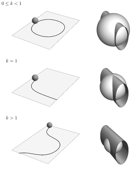
Figure 3.1. On the right are intersections of the elliptic-cylinder $H_{\text{SR}}=1/2$ with coadjoint orbits in $\mathfrak{so}(3)^{*}$. The corresponding paths which the ball traces on the table are shown on the left.

Remark 3.1.

The rolling problem we have discussed is related to an interview question asked in the 1950s at the University of Oxford [13], first solved in [6] (see also [18]). Given two points $p_{0}$ and $p_{1}$ on the table, and two configurations $g_{0}$ and $g_{1}$ of the ball, what is the shortest length path which rolls $(p_{0},g_{1})$ to $(p_{1},g_{1})$? Our problem differs from this in two respects. Firstly, we do not care about connecting two points on the table, only the two configurations of the ball, and secondly, the metric on the table is non-Euclidean. It is curious to compare the curves in equation (30) with those for the Euclidean case $J_{2}=J_{3}$ where the ball is found to travel across the table in straight lines and circular arcs.

4. Conclusion

We verified that our sub-Riemannian metric in the special orthogonal group $\mathbf{SO}(n)$ can be achieved as the limit of the Riemannian metric defined by the mass matrix. By computing the limit of the Manakov integrals, we found the constants of motion for the sub-Riemannian geodesic flow, which suggested the existence of a Lax Pair formulation for the sub-Riemannian geodesic equations. We used the bi-Hamiltonian structure to show the sub-Riemannian Manakov integrals are in involutions, and we proved that they are linearly independent. Therefore, the sub-Riemannian geodesic flow in $\mathbf{SO}(n)$ is Liouville integrable if the sub-Riemannian metric satisfies the condition $0<I_{2}<\dots<I_{n}$.

Future work includes the following:

1. Study the abnormal geodesics in $\mathbf{SO}(n)$ for $n>3$. We remark that $\operatorname{SO}(3)$ has the structure of a contact manifold, and it is known that every contact manifold does not have abnormal geodesics; consult [2, Proposition 4.38] or [25, sub-Chapter 5.2]. Therefore, the problem is not trivial for $n>3$.

2. Classify the relative equilibrium points of the sub-Riemannian geodesic flow on $\mathbf{SO}(n)$, consult [15] for the Riemannian case.

3. In [11, 12], V. Dragović, B. Cajić, and B. Jovanović studied the singular Manakov flow, i.e., the case when some of the values $J_{i}$ in the mass matrix $J$ are equal. This condition implies that the generalized rigid body is symmetric, making the Hamiltonian system invariant under the right multiplication of a sub-group $\mathbf{SO}(n)_{J}$ of $\mathbf{SO}(n)$, refer to [11] for more details about the construction of $\mathbf{SO}(n)_{J}$. These extra symmetries make the set of Manakov integrals linearly dependent and they are not enough to prove the Riemannian geodesic flow is Liouville integrable. However, the induced symmetry by $\mathbf{SO}(n)_{J}$ defines a momentum map, providing enough constants of motion to show that the Riemannian geodesic flow is non-commutatively integrable. We believe that the sub-Riemannian singular flow is non-commutatively integrable.

4. Consider new sub-Riemannian structures in semi-simple Lie groups and study the integrability of the system, consult [30]. For instance, in [29], T. Ratiu and D. Tamara study the Riemannian geodesic flow on $SU(n)$.

Appendix A Background

This Section introduces the fundamental definition and results used during the work.

A.1. Poisson structure

Let $Q$ be a smooth manifold, a Poisson structure in $Q$ is a bi-linear operator $\{\cdot,\cdot\}$ on the space of smooth functions $C^{\infty}(Q)$ from $Q$ to $\mathbb{R}$, with the property that the pair $(C^{\infty}(Q),\{\;,\;\})$ is a Lie algebra and $\{\;,\;\}$ is a derivation in each factor, i.e., for all $F,G$ and $H$ in $C^{\infty}(Q)$ the following expression holds

$$\{FG,H\}=\{F,H\}G+F\{G,H\}$$

Every Poisson structure in $Q$ induce a Poisson tensor $P_{Q}:T^{*}Q\to TQ$ such that

$$\{f,g\}=<dF,P_{Q}d_{m}g>,$$

where $<\;,\;>$ is the pairing. Then the Hamiltonian vector field $X_{H}$ for a Hamiltonian function $H$ defined by the Poisson structure is given by $X_{H}:=P_{M}dH$. Refer to [21, Chapter 10] for more details about the Poisson structure.

We say that two points $q_{1}$ and $q_{2}$ in Poisson manifold $Q$ are related if there is a piecewise smooth curve in $Q$ joining $q_{1}$ and $q_{2}$, each segment of which is a trajectory of locally Hamiltonian vector fields. This relation defines an equivalence relation, and an equivalence class is called a symplectic leaf. The Symplectic Stratification Theorem, consult [21, Theorem 10.4.4], states that if $Q$ is a finite-dimensional Poisson manifold, then $Q$ is the disjoint union of its symplectic leaf.

Let $F$ and $G$ be in $C^{\infty}(Q)$, we say that $F$ and $G$ are in involution (or Poisson commute) if $\{F,G\}=0$. If $F$ and $G$ Poisson commute, then $G$ is constant along the flow of the Hamiltonian vector field $X_{F}$, and we call $G$ a constant of motion of the Hamiltonian flow. We say that a family of functions $\{F_{1},\dots,F_{m}\}$ is involutive if any two elements are in involution. A classic result in Poisson geometry is the following: if $\{F_{1},\dots,F_{m}\}$ is an involutive family of function, then the vector fields $\{X_{F_{1}},\dots,X_{F_{1}}\}$ commute with respect the vector field bracket, consult [1, Proposition 4.4].

We say that a family of function $\{F_{1},\dots,F_{m}\}$ is linearly independent if the open subset on which the set of differential $\{dF_{1},\dots,dF_{m}\}$ are independent is dense in $M$.

The Poisson manifold has a distinguished family of functions with the property that Poisson commutes with every function $C^{\infty}(Q)$. Let us formalize: we say that a function $C$ is a Casimir if $C$ Poisson commute with every $F$ in $C^{\infty}(Q)$; in other words, $C$ is constant along the flow of all Hamiltonian vector fields. Another characterization of the Casimir function is a function $C$, whose differential $dC$ is in the kernel of the Poisson tensor, i.e., $P_{Q}dC=0$. Then, the number of linearly independent Casimir functions at a point $q$ is equal to the kernel of $P_{Q}|_{q}$. Given a point $q$ in $Q$, the dimension of the symplectic leaf is equal to $dim\;Q-dim\;KerP_{Q}|_{q}$. The only Casimir functions on a symplectic manifold are the constant functions, so every symplectic manifold only has one symplectic leaf.

Let $Q$ be a Poisson manifold with a symplectic leaf of dimension $2r$, we say that a family of functions $\{h_{1},\dots,h_{m}\}$ is Liouville integrable if it is involutive and independent with $m=dim\;Q-r$, refer to [1, Definition 4.13]. We notice that to a system is integrable on a symplectic leaf of dimension $2r$ is is enough to find the $r$ constants of motion besides the Casimir function.

A.1.1. Lax Pair

The existence of a Lax pair is a powerful tool for finding the constant of motion. This concept emerged from modern studies of integrable systems. Consider a Poisson manifold $Q$ and a Hamiltonian function $H$. A Lax pair $(M,\Omega)$ consists of two matrix functions $M$ and $\Omega$ from $Q$ to $\mathfrak{gl}$, such that the Hamiltonian equations defined by $H$ are equivalent to the following equation

$$\dot{M}=[M,\Omega],$$

where $[M,\Omega]$ denotes the commutator of the matrices $M$ and $L$.

The interest in the existence of a Lax pair lies in the fact that it provides constants of motion, such as the eigenvalues of $M$ and a trace of $M^{k}$ for all natural numbers $k$. We summarize this in the following Lemma.

Lemma A.1.

Let $M$ and $\Omega$ be a Lax pair satisfying $\dot{M}=[M,\Omega]$, then $Tr(M^{k})$ is a constant of motion for all natural number $n$.

For the proof of the above Lemma and more details about the Lax pair, consult [1].

A.2. Geodesic flow on Lie groups with left-invariant metrics

We will summarize some of the fundamental results on geodesic flow on Lie groups with left-invariant metrics, refer to [5, Appendix 2] or [21, Chapter 4] for more details.

Let $\mathbb{G}$ be Lie group, and let $L_{g}$ be the left translation by an element $g$ in $\mathbb{G}$, we say that a Riemannian metric is left-invariant it is preserved by all the left translations $L_{g}$, i.e., if every vector $v$ in $\mathfrak{g}$ has the same length than $(L_{g})_{*}v$ for every $g$, where $(L_{g})_{*}$ is the pull-forward. In the case of the classic rigid body (where the group is $\operatorname{SO}(3)$), the left-invariant metric implies that the angular velocity of the body determines the kinetic energy of the body and does not depend on the position of the body in the space. We consider a Riemannian geodesic on an arbitrary Lie group with a left-invariant metric as the “generalized rigid body”, where $\mathbb{G}$ is the configuration space.

Let $\mathbb{G}$ be Lie group with a left-invariant Riemannian metric or Sub-Riemannian metric, then the actions of $\mathbb{G}$ by the left and the right on its self defined actions on $T^{*}\mathbb{G}$ (the co-lift action). These actions give corresponding momentum maps $J_{R}$ and $J_{L}$, where $J_{R}$ corresponds to the left trivialization and defines the Lie-Poisson reduction of $T^{*}\mathbb{G}$ by the left action, and $J_{L}$ corresponds to the right trivialization and form the momentum map for the left translation. The following diagram summarizes the above discussion.

The subscripts $\pm$ are for a plus or minus sign in front of the Lie-Poisson bracket on $\mathfrak{g}^{*}$ (also known as Kostant-Kirrilov-Souriau). We call the above diagram a dual pair, which illustrates the relation between the body and spatial description of the rigid body, consult [5, Chapter 6] or [21, Chapter 15].

The Lie-Poisson reduction Theorem, consult [21, Theorem 13.1.1], states that the identification of function on $\mathfrak{g}^{*}$ with the set of left-invariant functions on $T^{*}\mathbb{G}$ endows $\mathfrak{g}^{*}$ with the Poisson structure given by Lie-Poisson bracket, i.e., if $\mathbb{G}$ is a Lie group, then $\mathfrak{g}^{*}$ has a natural Poisson structure, called the Lie-Poisson structure, induced by the Lie bracket, i.e., if $F$ and $G$ are functions from $\mathfrak{g}^{*}$ to $\mathbb{R}$, and $[\;,\;]$ is the Lie-bracket, then the Lie-Poisson bracket is

(31) $$\{F(\mu),G(\mu)\}_{\text{\tiny L-P}}:=-<\mu,[dF,dG]>,\;\text{where}\;\mu\;\text{is in}\;\mathfrak{g}^{*}.$$

Let $H:T^{*}\mathbb{G}\to\mathbb{R}$ be a left-invariant Hamiltonian function under the co-lift action, as an example, the kinetic energy of a “generalized rigid body”, then symplectic leaf are invariant under the Hamiltonian flow. Restricting $H$ to the symplectic leaf, we define a reduced Hamiltonian system on a smaller dimensional space. Therefore, by studying its reduced systems, we can determine the Liouville integrability of the Hamiltonian system.

References

- [1] Mark Adler, Pierre Moerbeke, and Pol Vanhaecke. Algebraic Integrability, Painlevé Geometry and Lie Algebras, volume 47. 01 2004.
- [2] Andrei Agrachev, Davide Barilari, and Ugo Boscain. A Comprehensive Introduction to Sub-Riemannian Geometry. Cambridge University Press, 2019.
- [3] Andrei A Agrachev, A Stephen Morse, Eduardo D Sontag, Héctor J Sussmann, Vadim I Utkin, and Andrei A Agrachev. Geometry of optimal control problems and hamiltonian systems. Nonlinear and Optimal Control Theory: Lectures given at the CIME Summer School held in Cetraro, Italy June 19–29, 2004, pages 1–59, 2008.
- [4] Andrei A Agrachev and Yuri Sachkov. Control theory from the geometric viewpoint, volume 87. Springer Science & Business Media, 2013.
- [5] V. I. Arnold. Mathematical methods of classical mechanics, volume 60 of Graduate Texts in Mathematics. Springer-Verlag, New York, second edition, 1989. Translated from the Russian by K. Vogtmann and A. Weinstein.
- [6] A. M. Arthurs and G. R. Walsh. On Hammersley’s minimum problem for a rolling sphere. Math. Proc. Cambridge Philos. Soc., 99(3):529–534, 1986.
- [7] Paul F. B. and Morris D. F. Handbook of Elliptic Integrals for Engineers and Scientists. Grundlehren der mathematischen Wissenschaften. Springer Berlin, Heidelberg, 1971.
- [8] A.M. Bloch. Nonholonomic Mechanics and Control. Springer New York, 2003, 2015.
- [9] Anthony Bloch, Vasile Brînzănescu, Arieh Iserles, Jerrold Marsden, and Tudor Ratiu. A class of integrable flows on the space of symmetric matrices. Communications in Mathematical Physics, 290, 2009.
- [10] A. Bravo-Doddoli, E. Le Donne, and N. Paddeu. Symplectic reduction of the sub-riemannian geodesic flow for metabelian nilpotent groups. Geometric Mechanics, 2024.
- [11] V. Dragović, B. Gajić, and B. Jovanović. Singular Manakov flows and geodesic flows on homogeneous spaces of . Transform. Groups, 14(3):513–530, 2009.
- [12] B. Ga˘iich, V. Dragovićh, and B. ˘Iovanovich. On the completeness of Manakov integrals. Fundam. Prikl. Mat., 20(2):35–49, 2015.
- [13] J. M. Hammersley. Oxford commemoration ball. In Probability, statistics and analysis, volume 79 of London Math. Soc. Lecture Note Ser., pages 112–142. Cambridge Univ. Press, Cambridge-New York, 1983.
- [14] S. Helgason. Differential Geometry, Lie Groups, and Symmetric Spaces. Elsevier Science, 1979.
- [15] Antonio Hernández-Garduno, Jeffrey K Lawson, and Jerrold E Marsden. Relative equilibria for the generalized rigid body. Journal of Geometry and Physics, 53(3):259–274, 2005.
- [16] J. Hilgert and K.H. Neeb. Structure and Geometry of Lie Groups. Springer Monographs in Mathematics. Springer New York, 2011.
- [17] Frédéric Jean. Sub-riemannian geometry. Lectures given at SISSA, 2003.
- [18] Velimir Jurdjevic. Geometric control theory, volume 52 of Cambridge Studies in Advanced Mathematics. Cambridge University Press, Cambridge, 1997.
- [19] Boris S Kruglikov, Andreas Vollmer, and Georgios Lukes-Gerakopoulos. On integrability of certain rank 2 sub-riemannian structures. Regular and Chaotic Dynamics, 22:502–519, 2017.
- [20] Sergei Valentinovich Manakov. Note on the integration of euler’s equations of the dynamics of an -dimensional rigid body. Funktsional’nyi Analiz i ego Prilozheniya, 10(4):93–94, 1976.
- [21] Jerrold E Marsden and Tudor S Ratiu. Introduction to mechanics and symmetry: a basic exposition of classical mechanical systems, volume 17. Springer Science & Business Media, 2013.
- [22] A. S. Miščenko and A. T. Fomenko. Euler equation on finite-dimensional Lie groups. Izv. Akad. Nauk SSSR Ser. Mat., 42(2):396–415, 471, 1978.
- [23] Felipe Monroy-Pérez and Alfonso Anzaldo-Meneses. Integrability of nilpotent sub-Riemannian structures. PhD thesis, INRIA, 2003.
- [24] Richard Montgomery. Abnormal minimizers. Siam Journal on control and optimization, 32(6):1605–1620, 1994.
- [25] Richard Montgomery. A tour of subriemannian geometries, their geodesics and applications, volume 91 of Mathematical Surveys and Monographs. American Mathematical Society, Providence, RI, 2002.
- [26] Carlo Morosi and Livio Pizzocchero. On the euler equation: Bi-hamiltonian structure and integrals in involution. Letters in Mathematical Physics, 37, 1996.
- [27] Lev Semenovich Pontryagin. Mathematical theory of optimal processes. Routledge, 2018.
- [28] Tudor Ratiu. The motion of the free -dimensional rigid body. Indiana University Mathematics Journal, 29, 1980.
- [29] Tudor S Ratiu and Daisuke Tarama. The u (n) free rigid body: Integrability and stability analysis of the equilibria. Journal of Differential Equations, 259(12):7284–7331, 2015.
- [30] Tudor S Ratiu and Daisuke Tarama. Geodesic flows on real forms of complex semi-simple lie groups of rigid body type. Research in the Mathematical Sciences, 7:1–37, 2020.