Scale Contrastive Learning with Selective Attentions for Blind
Image Quality Assessment

Abstract

Blind image quality assessment (BIQA) serves as a fundamental task in computer vision, yet it often fails to consistently align with human subjective perception. Recent advances show that multi-scale evaluation strategies are promising due to their ability to replicate the hierarchical structure of human vision. However, the effectiveness of these strategies is limited by a lack of understanding of how different image scales influence perceived quality. This paper addresses two primary challenges: the significant redundancy of information across different scales, and the confusion caused by combining features from these scales, which may vary widely in quality. To this end, a new multi-scale BIQA framework is proposed, namely Contrast-Constrained Scale-Focused IQA Framework (CSFIQA). CSFIQA features a selective focus attention mechanism to minimize information redundancy and highlight critical quality-related information. Additionally, CSFIQA includes a scale-level contrastive learning module equipped with a noise sample matching mechanism to identify quality discrepancies across the same image content at different scales. By exploring the intrinsic relationship between image scales and the perceived quality, the proposed CSFIQA achieves leading performance on eight benchmark datasets, e.g., achieving SRCC values of 0.967 (versus 0.947 in CSIQ) and 0.905 (versus 0.876 in LIVEC).

1 Introduction

Image quality assessment (IQA) seeks to emulate the human visual system’s ability to perceive image quality (Yang et al. 2022; Zhang et al. 2022b). It has been extensively applied in image restoration (Zhang et al. 2022a), compression (Liu et al. 2022), and generation (Wang et al. 2023), thereby enhancing the human visual experience. Based on the need for distortion-free reference images, IQA can be categorized into three types: full-reference, reduced-reference, and no-reference or blind IQA (BIQA) (Liu et al. 2024; Chahine et al. 2023; Zhang et al. 2023). Among these, BIQA methods have seen a significant increase in demand due to their broad applicability.

Multi-scale methods are extensively employed in BIQA aiming at simulating the multi-scale perception characteristics of the human vision system (Guo et al. 2021). Numerous studies have validated the effectiveness of these approaches, which can be broadly classified into image-level and feature-level methods based on their strategies for extracting and fusing multi-scale features (Chen et al. 2024). Image-level methods, such as NIQE (Mittal, Soundararajan, and Bovik 2013) and MUSIQ (Ke et al. 2021a), typically create multi-scale images by directly resizing the original image, from which features are extracted, and quality scores are computed in parallel. However, it is straightforward that direct resizing can introduce additional distortions into the image. On the other hand, many existing methods focus on feature-level extraction (Golestaneh, Dadsetan, and Kitani 2022a; Xu et al. 2024), employing a pyramid structure to derive multi-scale spatial features from the same image for predicting the quality scores.

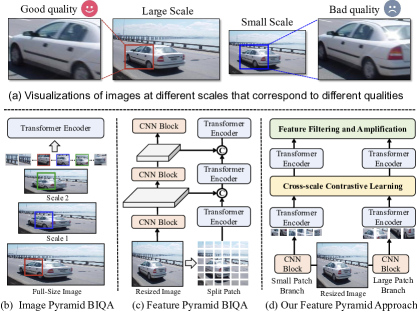
Figure 1: (a) The quality-aware information for a patch at the same relative position varies significantly across different image scales. At a small scale, overexposure on the cropped image patch greatly reduces the image quality, while at a larger scale, the quality of image patch remains relatively good. (b-d) Comparison of two mainstream multi-scale paradigms with our proposal. Our method leverages cross-scale contrastive learning to distinguish the quality differences in (a). The designed feature filtering and amplification module enhances attention to quality-aware features.

Despite the multi-scale BIQA methods achieving favourable results, they often struggle to accurately characterize the relationship between scale and the overall image quality. The reasons lie in two aspects: (1) Firstly, there exists a considerable degree of information redundancy across different scales, and processing this data indiscriminately can result in a significant waste of computational resources. (2) Secondly, feature-level multi-scale methods often directly concatenate features of different scales to predict quality scores. This approach can create a “visual illusio” effect, where the quality-aware information from different scales confuses the model’s ability to make an accurate assessment. This phenomenon is illustrated in Fig. 1(a) in which the same content photograph but different scales exhibit distinct quality differences. Specifically, the small-scale image contains overexposed lighting, leading to prominent low-quality areas. Consequently, the fusion of information at the scale level inevitably introduces noise into the quality perception features. To address these issues, we propose the Contrast-Constrained Scale-Focused IQA Framework (CSFIQA), an innovative methodology designed to minimize information redundancy while accurately simulating the complex relationship between scale and overall image quality.

To address the redundancy of multi-scale information highlighted in Problem 1, we propose an efficient selective focus attention mechanism to filter and enhance multi-scale quality information. This mechanism includes a filtering selector and an information focuser. The filtering selector identifies and retains the most relevant self-attention values from multi-scale features, while the information focuser amplifies these retained features, thereby reducing redundancy. As for Problem 2, accurately distinguishing quality perception information at different scales is crucial for alleviating visual illusions. Correspondingly, inspired by the effectiveness of contrastive learning in differentiating samples of varying quality, we propose a contrastive learning strategy that operates on both inter-scale and intra-scale levels to enhance the model’s ability in learning from quality perception features across scales. Specifically, we construct a straightforward set of positive and negative samples based on quality labels to capture more intricate relationships between different image quality regions. At the intra-scale level, we have designed a simple yet effective adaptive noise sample matching mechanism. We identify the sample in the neighboring region of scale B with the least similar quality information as a negative class for contrastive learning for a given image at scale A, thereby effectively distinguishing those cropped patches with inconsistent quality information across different scales of the same image.

We summarize our contributions:

• We identify the previously overlooked phenomenon in multi-scale BIQA methods and present a comprehensive analysis of the relationship between the patch scales and the overall image quality.

• We propose a selective focus attention mechanism that reduces redundancy in multi-scale information by filtering out highly correlated quality features and amplifying the retained features.

• We introduce the contrastive loss metrics across multiple scales to capture intricate relationships within diverse regions of image quality. Meanwhile, we propose a straightforward yet effective adaptive noise sample matching mechanism for collecting negative samples. This mechanism efficiently distinguishes samples that exhibit inconsistent quality information across different patch scales within the same image.

Extensive experiments conducted on eight IQA datasets reveal that our CSFIQA surpasses existing state-of-the-art BIQA approaches. Notably, in contrast to existing contrastive learning methods, we have identified quality inconsistencies across patch scales and introduced an adaptive noise sample matching mechanism to address these discrepancies.

2 Related Work

2.1 Deep Learning Based BIQA

Early deep learning-based Image Quality Assessment (IQA) methods utilized convolutional neural networks (CNNs) to extract features and learn the complex mapping between image features and quality (Zhang et al. 2018; Bosse et al. 2017; Hu et al. 2021). Despite the effective results they have achieved, these methods struggle to capture non-local information. To address this limitation, Vision Transformer (ViT)-based BIQA has gained significant attention in recent years due to ViT’s powerful capability in modelling non-local dependencies(Qin et al. 2023; Zhu et al. 2021). ViT-based NR-IQA methods generally fall into two categories: hybrid Transformers (Golestaneh, Dadsetan, and Kitani 2022b; Xu et al. 2024) and pure ViT-based Transformers (Yu et al. 2024). Hybrid Transformer methods utilize CNNs to extract perceptual features, which are then fed into Transformer encoders. However, CNNs may introduce information redundancy during the feedforward process. Pure ViT-based IQA methods typically use encoders to characterize image attributes across multiple patches. Nonetheless, the Transformer encoder’s cls token, initially designed for image content description, focuses on higher-level visual abstraction. Relying solely on the cls token may be insufficient for accurately representing image quality across different regions.

2.2 BIQA with Contrastive Learning

In recent years, unsupervised methods based on the principles of contrastive learning have been widely used in the BIQA field (Zhao et al. 2023; Li et al. 2024). CONTRIQUE (Madhusudana et al. 2022) was one of the first proposed, employing deep CNNs with contrastive paired objectives for quality representation. Re-IQA (Saha, Mishra, and Bovik 2023) utilized a mixture of experts to pre-train independent encoders for content and quality features, achieving remarkable results. However, these methods often use distortion types and levels as class labels for samples instead of using the actual quality labels of the images. Additionally, they uniformly treat images with different content as negative samples, lacking consideration for the relationship between quality regions of different images. We introduce scale contrastive learning to accurately model the relationship between different quality regions and the overall image quality.

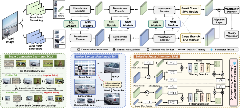
Figure 2: The overall of our CSFIQA. For a given input image, the $l$-th layer Transformer Encoder extracts image features $F^{l}_{a}$ ($a\in\{small,large\}$) at different scales. These features are then input into the SCL module (Sec. 3.2), which uses the relative distance of quality labels in the mini-batch to identify inter and intra-scale positive and negative samples for contrastive learning, enhancing the ability to discriminate quality differences between images. The NSM (Sec. 3.3) further selects the least similar quality patches within an image across different scales to address the “visual illusion” effect caused by varying quality information (see Fig. 1(a)). Features from the final encoder layer $F^{L}_{a}$ enter the SFA module (Sec. 3.3), where the Filtering Selector retains the Top-k similarity scores for self-attention, and the Information Concentrator amplifies important details to obtain quality-aware features. These features are then decoded to predict the quality $\hat{Y}$ (see Pseudocode 1 for more details).

3 Proposed Method

3.1 Overall Pipeline

In this paper, we present our framework CSFIQA, designed to precisely model the relationship between image scale and overall quality. As illustrated in Fig 2, our approach effectively integrates two primary modules: the Scale contrastive learning module (SCL) and the Selective Focus Attention module (SFA). Initially, the input image $I$ is segmented into patches of varying scales, denoted as $P_{s}$ and $P_{l}$. These patches are then independently processed through distinct $L$ layers of the Transformer encoder to extract scale-level features $F^{l}_{a}$ ($a\in\{small,large\}$) at the $l$-th layer. The scale-level features are subsequently forwarded to the SCL module at Sec. 3.2 to derive positive and negative samples, denoted as $P$ and $N$. They are utilized to compute their respective InfoNCE loss. Simultaneously, through an adaptive noise sample matching mechanism, we obtain the loss of the least similar quality patches within the same image and further penalize it. The output of the final encoder layer is passed to the SFA (Sec. 3.3). This mechanism generates features at different scales, which are then refined through an alignment layer and a Transformer decoder to produce the predicted quality scores (see Pseudocode 1 for more details).

3.2 Scale Contrastive Learning

To capture more complex relationships in different image quality regions, we introduce scale-level contrastive learning, improving upon previous methods. This approach utilizes loss to force scale-level features of quality regions belonging to the same (or different) quality to move closer together (or further apart), distinguishing samples with inconsistent quality information to varying scales of the same image. For $\forall\;F^{k_{i}}_{a}\in P$, we define scale-level contrastive loss as follows:

$${L}_{scale}=\sum_{k=1}^{K}\sum_{a\in\{s,l\}}\frac{1}{|P|}\sum_{F^{k}_{j}\in P}\mathcal{L}(F^{k_{i}}_{a},F^{k_{i^{+}}}_{a}),$$ (1)

where

$$\mathcal{L}(F^{k_{i}}_{a},F^{k_{i^{+}}}_{a})=\log\frac{-\exp(\frac{F^{k_{i}}_{a}\cdot F^{k_{i^{+}}}_{a}}{\tau})}{\exp(\frac{F^{k_{i}}_{a}\cdot F^{k_{i^{+}}}_{a}}{\tau})+\sum_{j\in N}\exp(\frac{F^{k_{i}}_{a}\cdot F^{k_{j}}_{a}}{\tau})}.$$ (2)

Here, $\tau$ denotes the temperature hyperparameter and $F^{k_{i}}_{a}$ represents the features of image $i$ at any scale in layer $k$ of the encoder. We set $\beta$ as our threshold to divide different positive and negative sample sets. As shown in Algorithm 1, for scale-level images $i$ and $j$, we define their positive and negative samples as follows:

$$\text{Classifier}(I_{i},I_{j})\in\begin{cases}$P$,&\text{if }|Y_{i}-Y_{j}|\leq\beta,\\ $N$,&\text{if }|Y_{i}-Y_{j}|>\beta.\end{cases}$$ (3)

Noise Sample Matching (NSM). We propose a simple yet effective adaptive noise sample matching mechanism to further distinguish samples with inconsistent quality information across different scales of the same image. We identify the sample in the neighbouring region at scale $s$ with the least similar quality information as a negative sample for contrastive learning for a given image at scale $l$. First, we divide the feature maps into quality regions for different scales.

Given a feature map $G_{a}\in\mathbb{R}^{H_{a}\times W_{a}\times D_{a}}$ at different scales, where $D_{a}$ represents the patch token and dimension, we use a sliding window $W_{a}\in\mathbb{R}^{H^{\prime}_{a}\times W^{\prime}_{a}}$ to divide the image into different local regions. We define $M$ blocks obtained by partitioning at scale $s$ and $K$ blocks obtained by partitioning at scale $l$. For each region $G^{m}_{small}$ at scale $s$, we compute its cosine similarity with each region $G^{k}_{large}$ at scale $l$:

$$Sim(G^{m}_{small},G^{k}_{large})=\frac{G^{m}_{small}\cdot G^{k}_{large}}{\|G^{m}_{small}\|\|G^{k}_{large}\|}.$$ (4)

We compute the loss across all regions that satisfy the specified criteria on $s$-scale feature maps in eq 4. This approach enables us to differentiate samples that exhibit inconsistent quality information across various scales for the same image:

$${L}_{noise}=\sum_{m=1}^{M}\sum_{k=1}^{K}\frac{1}{Sim(G^{m}_{small},G^{k}_{large})}.$$ (5)

Overall Loss. Let $\hat{Y}$ and $Y$ respectively denote the predicted scores and the ground truth scores for the image $I$. Given $\lambda$ represent the hyperparameters. The notation $\|\cdot\|_{1}$ signifies the $\ell_{1}$ regression loss. The total loss is defined as:

$$\mathcal{L}=\sum_{I}\left(\left\|\hat{Y}-Y\right\|_{1}+\lambda\left({L}_{scale}+{L}_{noise}\right)\right).$$ (6)

3.3 Selective Focus Attention

We revisit the cross-attention module widely used in most multi-scale models. Given different branches $l$ and $s$, the cls token from the $l$ branch is first concatenated with the patch token from the $s$ branch:

$$\begin{split}x^{\prime}&=\left[x^{l}_{\text{cls}},x^{s}_{\text{patch}}\right],\\ CrossAtt(x^{\prime})&=softmax\left(\frac{QK^{T}}{\sqrt{C/h}}\right)V.\end{split}$$ (7)

Here, $C$ represents the number of channels, and $h$ denotes the number of heads. Given $Q=x^{\prime}_{\text{cls}}W_{q}$, $K=x^{\prime}W_{k}$, and $V=x^{\prime}W_{v}$, this enables the fusion of cross-scale features. Our task is to accurately model the relationship between scale and overall image quality. However, this method may lead to information redundancy, potentially overlooking truly important quality information. This paper introduces a selective focusing module to replace it, which consists of an adaptive filtering selector and an information focuser. The adaptive filtering selector employs a filtering attention mechanism across different scales, utilizing the top-k similarity scores between cross-scale queries and key-values for information selection. The information localizer consists of a learnable linear layer and a frozen large language model layer, designed to focus on the quality content within the already filtered information. This approach reduces redundancy during the interaction process.

Algorithm 1 Pseudocode for proposed CSFIQA

Input: Mini-batch Images $I=\{X_{i},Y_{i}\}^{B}_{i=1}$
Variables:
      $B$: Batch size
      $F^{i}_{a}$: The large or small scale features of image $i$
      $P$: Positive pairs
      $N$: Negative pairs
      $M$: The number of regions divided at a small scale by NSM
      $K$: The number of regions divided at a large scale by NSM

Output: Predicted quality score $\{\hat{Y}\}^{B}_{i=1}$

1:  for  l, blk in enumerate(blocks) do

2:       // Transformer encoder

3:     for $i=1$ to $B$ do

4:        Calculate the $N$ and $P$ pairs by Eq.3

5:        $\mathcal{L}(F^{i}_{a},F^{i^{+}}_{a})=\log\frac{-\exp(F^{i}_{a}\cdot F^{i^{+}}_{a}/\tau)}{\exp(F^{i}_{a}\cdot F^{i^{+}}_{a}/\tau)+\sum_{j\in N}\exp(F_{a}^{i}\cdot F_{a}^{j}/\tau)}$

6:        $L_{\text{scale}}=L_{\text{scale}}+\mathcal{L}(F^{i}_{a},F^{i^{+}}_{a})$

7:        for $m=1$ to $M$ do

8:           for $k=1$ to $K$ do

9:              $Sim(G^{m}_{small},G^{k}_{large})=\frac{G^{m}_{small}\cdot G^{k}_{large}}{\|G^{m}_{small}\|\|G^{k}_{large}\|}$

10:              $L_{noise}$ = $L_{noise}$ + $\frac{1}{\exp(Sim(G^{m}_{small},G^{k}_{large})}$

11:           end for

12:        end for

13:     end for

14:       // Selective Focus Attention

15:     $F_{a}=SFA(F^{i}_{a})$

16:  end for

17:  Obtain $F$ from $F_{a}$ through the Alignment Layer

18:  $\hat{Y}=Decoder(F)$  // Transformer decoder

19:  $\mathcal{L^{\prime}}=\left(\left\|\hat{Y}-Y\right\|_{1}+\lambda\left(L_{scale}+L_{noise}\right)\right)$

Adaptive Filtering Selector (AFS). We follow the approach outlined in Eq. 7 for the computation of the attention matrix and for $Q$, $K$, and $V$. However, we implement an adaptive filtering top-k scale attention method across the channels for the final attention matrix to filter out redundant information and retain the most helpful attention values from multi-scale features. Expressly, we set up three learnable filtering masks, with their top-k values serving as filtering criteria drawn from the range [$\alpha$, $\beta$]. Only the top-k values of each row in the attention matrix that fall within the range [$\alpha$, $\beta$] will undergo normalization through softmax computation; otherwise, they will be replaced with 0. Finally, the attention matrix is obtained through a weighted average. Our filtering mechanism is defined as follows:

$$SelectAtt(Q,K,V)=\text{softmax}\left(\mathcal{M}_{k}\left(\frac{{Q}{K}^{\top}}{\sqrt{d_{k}}}\right)\right)V.$$ (8)

	LIVE		CSIQ		TID2013		KADID		LIVEC		KonIQ		LIVEFB		SPAQ
Method	PLCC	SRCC	PLCC	SRCC	PLCC	SRCC	PLCC	SRCC	PLCC	SRCC	PLCC	SRCC	PLCC	SRCC	PLCC	SRCC
BRISQUE  (Mittal, Moorthy, and Bovik 2012)	0.944	0.929	0.748	0.812	0.571	0.626	0.567	0.528	0.629	0.629	0.685	0.681	0.341	0.303	0.817	0.809
ILNIQE  (Zhang, Zhang, and Bovik 2015)	0.906	0.902	0.865	0.822	0.648	0.521	0.558	0.534	0.508	0.508	0.537	0.523	0.332	0.294	0.712	0.713
BIECON  (Kim and Lee 2016)	0.961	0.958	0.823	0.815	0.762	0.717	0.648	0.623	0.613	0.613	0.654	0.651	0.428	0.407	-	-
MEON  (Ma et al. 2017)	0.955	0.951	0.864	0.852	0.824	0.808	0.691	0.604	0.710	0.697	0.628	0.611	0.394	0.365	-	-
DBCNN  (Zhang et al. 2018)	0.971	0.968	0.959	0.946	0.865	0.816	0.856	0.851	0.869	0.851	0.884	0.875	0.551	0.545	0.915	0.911
TIQA  (You and Korhonen 2021)	0.965	0.949	0.838	0.825	0.858	0.846	0.855	0.85	0.861	0.845	0.903	0.892	0.581	0.541	-	-
MetaIQA  (Zhu et al. 2020)	0.959	0.960	0.908	0.899	0.868	0.856	0.775	0.762	0.802	0.835	0.856	0.887	0.507	0.54	-	-
P2P-BM  (Ying et al. 2020)	0.958	0.959	0.902	0.899	0.856	0.862	0.849	0.84	0.842	0.844	0.885	0.872	0.598	0.526	-	-
HyperIQA  (Su et al. 2020)	0.966	0.962	0.942	0.923	0.858	0.840	0.845	0.852	0.882	0.859	0.917	0.906	0.602	0.544	0.915	0.911
MUSIQ  (Ke et al. 2021b)	0.911	0.940	0.893	0.871	0.815	0.773	0.872	0.875	0.828	0.785	0.928	0.916	0.661	0.566	0.921	0.918
TReS  (Golestaneh, Dadsetan, and Kitani 2022a)	0.968	0.969	0.942	0.922	0.883	0.863	0.858	0.859	0.882	0.859	0.928	0.915	0.625	0.554	-	-
DACNN  (Pan et al. 2022)	0.980	0.978	0.957	0.943	0.889	0.871	0.905	0.905	0.884	0.866	0.912	0.901	-	-	0.921	0.915
Re-IQA  (Saha, Mishra, and Bovik 2023)	0.971	0.970	0.96	0.947	0.861	0.804	0.885	0.872	0.854	0.84	0.923	0.914	-	-	0.925	0.918
DEIQT  (Qin et al. 2023)	0.982	0.980	0.963	0.946	0.908	0.892	0.889	0.887	0.894	0.875	0.914	0.907	0.663	0.571	0.923	0.919
LoDa  (Xu et al. 2024)	0.979	0.975	-	-	0.901	0.869	0.936	0.931	0.899	0.876	0.944	0.932	0.679	0.578	0.928	0.925
CSFIQA (ours)	0.983	0.982	0.973	0.967	0.917	0.899	0.913	0.908	0.922	0.905	0.944	0.92	0.701	0.629	0.935	0.925

Table 1: Performance comparison measured by averages of SRCC and PLCC, where the bold entries indicate the best and the second best results for each dataset.

Information Concentrator Model (ICM). Recent work has shown that frozen LLM encoders can discern information-rich visual tokens and further enhance their contributions to latent representations (Pang et al. 2023). In our approach, we have implemented filtering of features at the scale level before inputting them into the frozen LLM layer. As a result, the frozen LLM layer functions as a scale information amplifier, exhibiting a stronger focus on the feature content that we consider essential.

4 Experiments

4.1 Datasets and Evaluation Protocols

We evaluated the CSFIQA on eight public Image Quality Assessment (IQA) datasets. Among these, LIVEC (Ghadiyaram and Bovik 2015), KonIQ-10k (Hosu et al. 2020), LIVEFB (Ying et al. 2020), and SPAQ (Fang et al. 2020) contain real distortions, while LIVE (Sheikh, Sabir, and Bovik 2006), CSIQ (Larson and Chandler 2010), TID2013 (Ponomarenko et al. 2015), and KADID (Lin, Hosu, and Saupe 2019) feature synthetic distortions. Specifically, the LIVEC dataset includes 1,162 images with diverse authentic distortions, while KonIQ-10k comprises 10,073 images from open multimedia resources. LIVEFB is the largest real distortion dataset, consisting of 39,810 images, and SPAQ contains 11,125 images from 66 smartphones. Synthetic datasets usually have a limited number of original images with distortions like Gaussian blur and JPEG compression applied. The LIVE and CSIQ datasets contain 779 and 866 synthetic images, respectively, covering 5 and 6 types of distortions. TID2013 and KADID offer a broader range, with 3,000 and 10,125 images featuring 24 and 25 distortion types, respectively. We used the Spearman Rank Correlation Coefficient (SRCC) and Pearson Linear Correlation Coefficient (PLCC) to evaluate monotonicity and accuracy, with values ranging from -1 to 1, where values close to 1 indicate excellent predictive performance.

4.2 Implementation Details and Setups

We employ a pre-trained encoder based on CrossViT (Chen, Fan, and Panda 2021) as our scale encoder. The encoder has an overall depth of 4, with the small-scale encoder having a depth of 1 and the large-scale encoder having a depth of 4. The decoder’s depth is set to 1. Different scales have resolutions of 384 and 224, with patch sizes of 12 and 16 and input token dimensions of 192 and 384, respectively. The number of heads is 6. The model was trained for 9 epochs with a learning rate 2e-4 and a decay factor of 10 applied every 3 epochs. Batch sizes range from 16 to 128, depending on the dataset size. The dataset was divided into 80% for training and 20% for testing, and this process was repeated ten times to minimize performance bias. We report the median SRCC and PLCC to evaluate the model’s prediction accuracy and monotonicity performance. All experiments were conducted based on the PyTorch framework, on two Linux servers each equipped with eight NVIDIA RTX 3090 GPUs.

4.3 Performance Comparison with SOTA

The results presented in Tab. 1 provide a comprehensive comparison between our proposed CSFIQA and 16 classical and state-of-the-art (SOTA) Blind Image Quality Assessment (BIQA) methods. These methods encompass hand-crafted feature-based BIQA techniques, such as BRISQUE and ILNIQE, and deep learning-based approaches, including DEIQT and LoDa. As observed in six of the eight datasets, CSFIQA outperforms all other methods in terms of performance. Since these datasets encompass a wide range of distortion types and image content, achieving leading performance across them is challenging. Consequently, these observations confirm the effectiveness and superiority of our model in accurately characterizing image quality.

4.4 Generalization Capability Validation

To evaluate the generalization capability of CSFIQA, we conducted cross-dataset validation experiments. The model is trained on one dataset and tested on others without parameter adjustments in these experiments. The results in Tab. 2 show the average SRCC across five datasets. Notably, CSFIQA performed best in all cross-dataset validations, including solid results on the LIVEC and KonIQ datasets. These outcomes are attributed to our scale-level contrastive learning module’s extensive scale information and the filtering and focusing power of the information enhancement module, highlighting the exceptional generalization ability of the CSFIQA model.

Training	LIVEFB		LIVEC	KonIQ	LIVE	CSIQ
Testing	KonIQ	LIVEC	KonIQ	LIVEC	CSIQ	LIVE
DBCNN	0.716	0.724	0.754	0.755	0.758	0.877
P2P-BM	0.755	0.738	0.740	0.770	0.712	-
TReS	0.713	0.74	0.733	0.786	0.761	-
DEIQT	0.733	0.781	0.744	0.794	0.781	0.932
LoDa	0.763	0.805	0.745	0.811	-	-
ours	0.785	0.805	0.762	0.838	0.786	0.933

Table 2: SRCC on the cross datasets validation. The best performances are highlighted in boldface.

4.5 Ablation study

Effect of Scale Contrastive learning Module (SCL). Our SCL comprises three main parts: inter-scale and intra-scale contrastive learning modules and the Selective Focus Attention Module (SFA). In Tab. 3 and Tab. 4, we conduct ablation experiments to compare the results of these modules on LIVEC and CSIQ datasets averaging over 10 trials. Tab. 3 outlines a baseline model DEIQT, with the second row incorporating the cross-scale module. The third row shows the results with the inclusion of the SCL module, while Tab. 4 details the results of each component.

Specifically, compared to the baseline, the improvement in the first row of Tab. 4 demonstrates the effectiveness of contrastive learning proposed in previous work. However, this alone is insufficient to address our challenges. The second row of Tab. 4 illustrates the effectiveness of scale information. We capture more complex relationships in different image quality regions by introducing cross-scale quality information at the same scale level. Additionally, the Adaptive Noise Sample Matching Mechanism (NSM) results suggest that refining quality information to a regional level in contrastive learning is beneficial. This refinement enhances the model’s capability to differentiate samples with inconsistent quality information across varying scales within a single image.

Effect of Selective Focus Attention (SFA). We also conducted ablation studies on the Selective Focus Attention (SFA) module, with the results in Tab. 3 and Tab. 4. These tables illustrate the performance of the module and its various components. Specifically, compared to the baseline, our method underscores the importance of eliminating redundant information, as such information is detrimental to quality assessment. The last row in Tab. 4 supports this observation: when redundant information is amplified without SFA, the CSIQ dataset’s performance falls below the baseline. Conversely, employing SFA alone leads to a marked improvement over the baseline. The results in Tab. 3 demonstrate that the AFS and ICM modules are complementary, and their integration yields optimal effectiveness.

Effect of weight $\lambda$. We conducted ablation experiments on the LIVEC and CSIQ datasets to examine the impact of the weight $\lambda$ in Eq. 6. As shown in Tab. 5, the results indicate that a larger $\lambda$ significantly affects gradients, leading to reduced performance. We used a $\lambda$ of 0.01 in our experiments based on our balanced observations.

Method				LIVEC		CSIQ
baseline	CrossViT	SCL	SFA	PLCC	SRCC	PLCC	SRCC
✔				0.892	0.872	0.959	0.94
✔	✔			0.896	0.878	0.964	0.948
✔	✔	✔		0.911	0.892	0.97	0.963
✔	✔		✔	0.904	0.887	0.965	0.956
✔	✔	✔	✔	0.922	0.905	0.973	0.967

Table 3: Ablation experiments on different modules. The best performances are highlighted in bold.

Method	Modules	LIVEC		CSIQ
		PLCC	SRCC	PLCC	SRCC
w/ SCL	inter-SCL	0.899	0.883	0.965	0.951
	intra-SCL	0.902	0.883	0.965	0.954
	NSM	0.903	0.887	0.967	0.958
w/ SFA	AFS	0.902	0.884	0.963	0.953
	ICM	0.901	0.878	0.96	0.949

Table 4: Ablation experiments with different components on two datasets. The best performances are highlighted in boldface.

	LIVEC		CSIQ
hyperparameter $\lambda$	PLCC	SRCC	PLCC	SRCC
0.1	0.915	0.9	0.969	0.956
0.01	0.922	0.905	0.973	0.967
0.001	0.910	0.887	0.966	0.954
0.0001	0.909	0.893	0.964	0.959

Table 5: The ablation study about soft weight $\lambda$.

Effect of weight $[\alpha,\beta]$. We performed ablation experiments on the threshold range $[\alpha,\beta]$ within the proposed AFS module, as presented in Tab. 6. It was observed that the choice of $k$ is a critical factor in setting boundaries for effective information filtering. Initially, $k$ was assigned a single value, and at $k=1/2$, performance showed high sensitivity. To avoid limited enumeration, we defined a range threshold and uniformly sampled values within this range for multiple masks. The best results were achieved when $[\alpha,\beta]$ was set to $[1/3,3/4]$. As $k$ continues to increase, the sampling range becomes denser, introducing noise and gradually degrading performance.

	LIVEC		CSIQ
soft weight $[\alpha,\beta]$	PLCC	SRCC	PLCC	SRCC
$[1/2]$	0.899	0.872	0.964	0.953
$[1/6,1/3]$	0.903	0.885	0.965	0.955
$[1/5,1/2]$	0.906	0.891	0.972	0.960
$[1/4,2/3]$	0.908	0.890	0.964	0.959
$[1/3,3/4]$	0.922	0.905	0.973	0.967
$[1/2,4/5]$	0.916	0.898	0.968	0.962

Table 6: The ablation study on the selection range [$\alpha$, $\beta$] in AFS module.

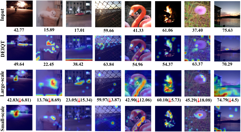
Figure 3: Activation maps of DEIQT  (Qin et al. 2023) and CSFIQA using Grad-CAM  (Selvaraju et al. 2017a) on authentic dataset LIVEC. The scores below the first row of images represent Mean Opinion Scores (MOS). Our model pays more attention to image distortion regions, and correspondingly our image quality prediction ability is closer to the true value. Rows 1-4 represent input images, CAMs from DEIQT, and CAMs from Large and small scale branch in CSFIQA, respectively.

4.6 Qualitative Analysis

We use GradCAM (Selvaraju et al. 2017b) to generate visual representations of the feature attention maps for the input images in our baseline model and CSFIQA, as shown in Fig. 3. We observe that different scale encoders have varying degrees of focus on image quality regions, highlighting the importance of modeling the relationship between scale and overall image quality. On the other hand, our proposed CSFIQA significantly outperforms the baseline model because it better utilizes inter-scale information to perceive image distortions. In contrast, the baseline model is more prone to incorrectly focusing on non-distorted areas and exhibits “visual illusions”. Our approach captures the complex relationships of different image quality regions, effectively extracting quality-aware features. Prediction results indicate that our method surpasses the baseline model across different distortion levels. However, the last two columns of our model demonstrate failure cases on the small-scale. Due to scale limitations, the small-scale encoder inevitably introduces some noise, but the large-scale model performs well in distorted regions, further demonstrating the superiority of our method.

5 Conclusion

In this study, we introduce the Contrast-Constrained Scale-Focused IQA Framework (CSFIQA), designed to capture quality information across diverse regions of an image effectively. Unlike traditional models that merely concatenate scale information, CSFIQA leverages cross-scale contrastive learning to differentiate the varying quality within a single image. Additionally, we implement a selective focus attention mechanism to refine quality information. Experiments show that CSFIQA surpasses existing state-of-the-art methods, which potentially provides a new paradigm for multi-scale approaches.

References

- Bosse et al. (2017) Bosse, S.; Maniry, D.; Müller, K.-R.; Wiegand, T.; and Samek, W. 2017. Deep neural networks for no-reference and full-reference image quality assessment. IEEE Transactions on image processing, 27(1): 206–219.
- Chahine et al. (2023) Chahine, N.; Calarasanu, S.; Garcia-Civiero, D.; Cayla, T.; Ferradans, S.; and Ponce, J. 2023. An image quality assessment dataset for portraits. In Proceedings of the IEEE/CVF Conference on Computer Vision and Pattern Recognition, 9968–9978.
- Chen et al. (2024) Chen, C.; Mo, J.; Hou, J.; Wu, H.; Liao, L.; Sun, W.; Yan, Q.; and Lin, W. 2024. Topiq: A top-down approach from semantics to distortions for image quality assessment. IEEE Transactions on Image Processing.
- Chen, Fan, and Panda (2021) Chen, C.-F. R.; Fan, Q.; and Panda, R. 2021. Crossvit: Cross-attention multi-scale vision transformer for image classification. In Proceedings of the IEEE/CVF international conference on computer vision, 357–366.
- Fang et al. (2020) Fang, Y.; Zhu, H.; Zeng, Y.; Ma, K.; and Wang, Z. 2020. Perceptual quality assessment of smartphone photography. In Proceedings of the IEEE/CVF Conference on Computer Vision and Pattern Recognition, 3677–3686.
- Ghadiyaram and Bovik (2015) Ghadiyaram, D.; and Bovik, A. C. 2015. Massive online crowdsourced study of subjective and objective picture quality. IEEE Transactions on Image Processing, 25(1): 372–387.
- Golestaneh, Dadsetan, and Kitani (2022a) Golestaneh, S. A.; Dadsetan, S.; and Kitani, K. M. 2022a. No-reference image quality assessment via transformers, relative ranking, and self-consistency. In Proceedings of the IEEE/CVF Winter Conference on Applications of Computer Vision, 1220–1230.
- Golestaneh, Dadsetan, and Kitani (2022b) Golestaneh, S. A.; Dadsetan, S.; and Kitani, K. M. 2022b. No-reference image quality assessment via transformers, relative ranking, and self-consistency. In Proceedings of the IEEE/CVF winter conference on applications of computer vision, 1220–1230.
- Guo et al. (2021) Guo, H.; Bin, Y.; Hou, Y.; Zhang, Q.; and Luo, H. 2021. Iqma network: Image quality multi-scale assessment network. In Proceedings of the IEEE/CVF Conference on Computer Vision and Pattern Recognition, 443–452.
- Hosu et al. (2020) Hosu, V.; Lin, H.; Sziranyi, T.; and Saupe, D. 2020. KonIQ-10k: An ecologically valid database for deep learning of blind image quality assessment. IEEE Transactions on Image Processing, 29: 4041–4056.
- Hu et al. (2021) Hu, R.; Liu, Y.; Wang, Z.; and Li, X. 2021. Blind quality assessment of night-time image. Displays, 69: 102045.
- Ke et al. (2021a) Ke, J.; Wang, Q.; Wang, Y.; Milanfar, P.; and Yang, F. 2021a. Musiq: Multi-scale image quality transformer. In Proceedings of the IEEE/CVF international conference on computer vision, 5148–5157.
- Ke et al. (2021b) Ke, J.; Wang, Q.; Wang, Y.; Milanfar, P.; and Yang, F. 2021b. Musiq: Multi-scale image quality transformer. In Proceedings of the IEEE/CVF International Conference on Computer Vision, 5148–5157.
- Kim and Lee (2016) Kim, J.; and Lee, S. 2016. Fully deep blind image quality predictor. IEEE Journal of selected topics in signal processing, 11(1): 206–220.
- Larson and Chandler (2010) Larson, E. C.; and Chandler, D. M. 2010. Most apparent distortion: full-reference image quality assessment and the role of strategy. Journal of electronic imaging, 19(1): 011006.
- Li et al. (2024) Li, X.; Hu, R.; Zheng, J.; Zhang, Y.; Zhang, S.; Zheng, X.; Li, K.; Shen, Y.; Liu, Y.; Dai, P.; et al. 2024. Integrating Global Context Contrast and Local Sensitivity for Blind Image Quality Assessment. In Forty-first International Conference on Machine Learning.
- Lin, Hosu, and Saupe (2019) Lin, H.; Hosu, V.; and Saupe, D. 2019. KADID-10k: A large-scale artificially distorted IQA database. In 2019 Eleventh International Conference on Quality of Multimedia Experience (QoMEX), 1–3. IEEE.
- Liu et al. (2022) Liu, J.; Li, X.; Peng, Y.; Yu, T.; and Chen, Z. 2022. Swiniqa: Learned swin distance for compressed image quality assessment. In Proceedings of the IEEE/CVF Conference on computer vision and pattern recognition, 1795–1799.
- Liu et al. (2024) Liu, Y.; Zhang, B.; Hu, R.; Gu, K.; Zhai, G.; and Dong, J. 2024. Underwater image quality assessment: Benchmark database and objective method. IEEE Transactions on Multimedia.
- Ma et al. (2017) Ma, K.; Liu, W.; Zhang, K.; Duanmu, Z.; Wang, Z.; and Zuo, W. 2017. End-to-end blind image quality assessment using deep neural networks. IEEE Transactions on Image Processing, 27(3): 1202–1213.
- Madhusudana et al. (2022) Madhusudana, P. C.; Birkbeck, N.; Wang, Y.; Adsumilli, B.; and Bovik, A. C. 2022. Image quality assessment using contrastive learning. IEEE Transactions on Image Processing, 31: 4149–4161.
- Mittal, Moorthy, and Bovik (2012) Mittal, A.; Moorthy, A. K.; and Bovik, A. C. 2012. No-reference image quality assessment in the spatial domain. IEEE Transactions on image processing, 21(12): 4695–4708.
- Mittal, Soundararajan, and Bovik (2013) Mittal, A.; Soundararajan, R.; and Bovik, A. C. 2013. Making a “Completely Blind” Image Quality Analyzer. IEEE Signal Processing Letters, 20(3): 209–212.
- Pan et al. (2022) Pan, Z.; Zhang, H.; Lei, J.; Fang, Y.; Shao, X.; Ling, N.; and Kwong, S. 2022. Dacnn: Blind image quality assessment via a distortion-aware convolutional neural network. IEEE Transactions on Circuits and Systems for Video Technology, 32(11): 7518–7531.
- Pang et al. (2023) Pang, Z.; Xie, Z.; Man, Y.; and Wang, Y.-X. 2023. Frozen transformers in language models are effective visual encoder layers. arXiv preprint arXiv:2310.12973.
- Ponomarenko et al. (2015) Ponomarenko, N.; Jin, L.; Ieremeiev, O.; Lukin, V.; Egiazarian, K.; Astola, J.; Vozel, B.; Chehdi, K.; Carli, M.; Battisti, F.; et al. 2015. Image database TID2013: Peculiarities, results and perspectives. Signal processing: Image communication, 30: 57–77.
- Qin et al. (2023) Qin, G.; Hu, R.; Liu, Y.; Zheng, X.; Liu, H.; Li, X.; and Zhang, Y. 2023. Data-Efficient Image Quality Assessment with Attention-Panel Decoder. In Proceedings of the Thirty-Seventh AAAI Conference on Artificial Intelligence.
- Saha, Mishra, and Bovik (2023) Saha, A.; Mishra, S.; and Bovik, A. C. 2023. Re-IQA: Unsupervised Learning for Image Quality Assessment in the Wild. In Proceedings of the IEEE/CVF Conference on Computer Vision and Pattern Recognition, 5846–5855.
- Selvaraju et al. (2017a) Selvaraju, R. R.; Cogswell, M.; Das, A.; Vedantam, R.; Parikh, D.; and Batra, D. 2017a. Grad-cam: Visual explanations from deep networks via gradient-based localization. In Proceedings of the IEEE international conference on computer vision, 618–626.
- Selvaraju et al. (2017b) Selvaraju, R. R.; Cogswell, M.; Das, A.; Vedantam, R.; Parikh, D.; and Batra, D. 2017b. Grad-cam: Visual explanations from deep networks via gradient-based localization. In Proceedings of the IEEE international conference on computer vision, 618–626.
- Sheikh, Sabir, and Bovik (2006) Sheikh, H. R.; Sabir, M. F.; and Bovik, A. C. 2006. A statistical evaluation of recent full reference image quality assessment algorithms. IEEE Transactions on image processing, 15(11): 3440–3451.
- Su et al. (2020) Su, S.; Yan, Q.; Zhu, Y.; Zhang, C.; Ge, X.; Sun, J.; and Zhang, Y. 2020. Blindly assess image quality in the wild guided by a self-adaptive hyper network. In Proceedings of the IEEE/CVF Conference on Computer Vision and Pattern Recognition, 3667–3676.
- Wang et al. (2023) Wang, J.; Duan, H.; Liu, J.; Chen, S.; Min, X.; and Zhai, G. 2023. Aigciqa2023: A large-scale image quality assessment database for ai generated images: from the perspectives of quality, authenticity and correspondence. In CAAI International Conference on Artificial Intelligence, 46–57. Springer.
- Xu et al. (2024) Xu, K.; Liao, L.; Xiao, J.; Chen, C.; Wu, H.; Yan, Q.; and Lin, W. 2024. Boosting Image Quality Assessment through Efficient Transformer Adaptation with Local Feature Enhancement. In Proceedings of the IEEE/CVF Conference on Computer Vision and Pattern Recognition, 2662–2672.
- Yang et al. (2022) Yang, S.; Wu, T.; Shi, S.; Lao, S.; Gong, Y.; Cao, M.; Wang, J.; and Yang, Y. 2022. Maniqa: Multi-dimension attention network for no-reference image quality assessment. In Proceedings of the IEEE/CVF Conference on Computer Vision and Pattern Recognition, 1191–1200.
- Ying et al. (2020) Ying, Z.; Niu, H.; Gupta, P.; Mahajan, D.; Ghadiyaram, D.; and Bovik, A. 2020. From patches to pictures (PaQ-2-PiQ): Mapping the perceptual space of picture quality. In Proceedings of the IEEE/CVF Conference on Computer Vision and Pattern Recognition, 3575–3585.
- You and Korhonen (2021) You, J.; and Korhonen, J. 2021. Transformer for image quality assessment. In 2021 IEEE International Conference on Image Processing (ICIP), 1389–1393. IEEE.
- Yu et al. (2024) Yu, Z.; Guan, F.; Lu, Y.; Li, X.; and Chen, Z. 2024. Sf-iqa: Quality and similarity integration for ai generated image quality assessment. In Proceedings of the IEEE/CVF Conference on Computer Vision and Pattern Recognition, 6692–6701.
- Zhang et al. (2022a) Zhang, C.; Su, S.; Zhu, Y.; Yan, Q.; Sun, J.; and Zhang, Y. 2022a. Exploring and evaluating image restoration potential in dynamic scenes. In Proceedings of the IEEE/CVF Conference on Computer Vision and Pattern Recognition, 2067–2076.
- Zhang, Zhang, and Bovik (2015) Zhang, L.; Zhang, L.; and Bovik, A. C. 2015. A feature-enriched completely blind image quality evaluator. IEEE Transactions on Image Processing, 24(8): 2579–2591.
- Zhang et al. (2022b) Zhang, W.; Li, D.; Min, X.; Zhai, G.; Guo, G.; Yang, X.; and Ma, K. 2022b. Perceptual attacks of no-reference image quality models with human-in-the-loop. Advances in Neural Information Processing Systems, 35: 2916–2929.
- Zhang et al. (2018) Zhang, W.; Ma, K.; Yan, J.; Deng, D.; and Wang, Z. 2018. Blind image quality assessment using a deep bilinear convolutional neural network. IEEE Transactions on Circuits and Systems for Video Technology, 30(1): 36–47.
- Zhang et al. (2023) Zhang, W.; Zhai, G.; Wei, Y.; Yang, X.; and Ma, K. 2023. Blind image quality assessment via vision-language correspondence: A multitask learning perspective. In Proceedings of the IEEE/CVF conference on computer vision and pattern recognition, 14071–14081.
- Zhao et al. (2023) Zhao, K.; Yuan, K.; Sun, M.; Li, M.; and Wen, X. 2023. Quality-aware pre-trained models for blind image quality assessment. In Proceedings of the IEEE/CVF conference on computer vision and pattern recognition, 22302–22313.
- Zhu et al. (2020) Zhu, H.; Li, L.; Wu, J.; Dong, W.; and Shi, G. 2020. MetaIQA: Deep meta-learning for no-reference image quality assessment. In Proceedings of the IEEE/CVF Conference on Computer Vision and Pattern Recognition, 14143–14152.
- Zhu et al. (2021) Zhu, M.; Hou, G.; Chen, X.; Xie, J.; Lu, H.; and Che, J. 2021. Saliency-guided transformer network combined with local embedding for no-reference image quality assessment. In Proceedings of the IEEE/CVF International Conference on Computer Vision, 1953–1962.