Cut Your Losses
in Large-Vocabulary Language Models

Abstract

As language models grow ever larger, so do their vocabularies. This has shifted the memory footprint of LLMs during training disproportionately to one single layer: the cross-entropy in the loss computation. Cross-entropy builds up a logit matrix with entries for each pair of input tokens and vocabulary items and, for small models, consumes an order of magnitude more memory than the rest of the LLM combined. We propose Cut Cross-Entropy (CCE), a method that computes the cross-entropy loss without materializing the logits for all tokens into global memory. Rather, CCE only computes the logit for the correct token and evaluates the log-sum-exp over all logits on the fly. We implement a custom kernel that performs the matrix multiplications and the log-sum-exp reduction over the vocabulary in flash memory, making global memory consumption for the cross-entropy computation negligible. This has a dramatic effect. Taking the Gemma 2 (2B) model as an example, CCE reduces the memory footprint of the loss computation from 24 GB to 1 MB, and the total training-time memory consumption of the classifier head from 28 GB to 1 GB. To improve the throughput of CCE, we leverage the inherent sparsity of softmax and propose to skip elements of the gradient computation that have a negligible (i.e., below numerical precision) contribution to the gradient. Experiments demonstrate that the dramatic reduction in memory consumption is accomplished without sacrificing training speed or convergence.

https://github.com/apple/ml-cross-entropy

1 Introduction

Progress in large language models (LLMs) has been fueled in part by an increase in parameter count, context length, and vocabulary size (the number of tokens that can be used to represent the input). As LLMs grew, so did the associated infrastructure. Large mini-batch gradient descent (Goyal et al., 2017) combined with data-parallelism (Hillis & Steele, 1986) enabled the harnessing of increasing computational power. ZeRO (Rajbhandari et al., 2020) broke the dependence between the number of GPUs and the memory used for model parameters, gradients, and optimizer state. Activation checkpointing (Chen et al., 2016) reduced the amount of memory used for activations, supporting the development of deeper models. FlashAttention (Dao et al., 2022) reduced the memory used in self-attention from $O(N^{2})$ to $O(N)$, thereby supporting longer context windows. These improvements gradually shifted the memory consumption of LLM training to one single layer – the cross-entropy loss, whose memory footprint grows with the product of vocabulary size and number of tokens per batch. The cross-entropy loss is responsible for up to $90\%$ of the memory footprint of modern LLM training (see Fig. 1(a)). The problem grows only more acute with time, since even the largest contemporary vocabularies (e.g., 256K tokens) may benefit from further expansion (Tao et al., 2024).

We propose a cross-entropy implementation, Cut Cross-Entropy (CCE), that has a negligible memory footprint and scales to arbitrarily large vocabularies. Our key insight is that computation of the loss and its gradient only depends on a single log-probability, that of the ground-truth label. With an arithmetic reformulation, we decompose the cross-entropy loss into an index matrix multiplication over a single ground-truth label and a log-sum-exp operation over all vocabulary entries for each token. Each operation has small and well-defined inputs – the network embeddings and classifier matrix – and a single scalar output per token. Both operations do, however, rely on a large intermediate logit matrix that computes the score for each token and potential vocabulary entry. We show that there is no need to materialize this logit matrix in GPU memory. Instead, we compute logits as needed in SRAM in a series of custom CUDA kernels. The result is a cross-entropy computation that has negligible memory footprint, with no detrimental effect on latency or convergence. See Fig. 1(b) for a breakdown of memory savings and consequent batch size increases afforded by CCE.

(a) Regular cross-entropy

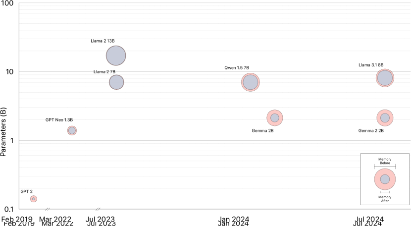
(b) Cut cross-entropy (ours)

Figure 1: Memory use and maximum attainable batch size (in millions of tokens) for a variety of frontier models on a 16-GPU (80 GB each) fully-sharded data-parallel setup (Rajbhandari et al., 2020) with activation checkpointing (Chen et al., 2016) and a mixed-precision 16-bit (fp16/bf16) AdamW optimizer (Kingma & Ba, 2015; Loshchilov & Hutter, 2019). For each model, we break its memory use down into weights and optimizer states, activation checkpoints, and the log-probabilities computed by the cross-entropy loss layer. Our Cut Cross-Entropy (CCE) enables increasing the batch size by 1.5x (Llama 2 13B) to 10x (GPT 2, Gemma 2 2B), with no sacrifice in speed or convergence. Exact values in Table A3.

2 Related Work

Attention mechanisms. The effectiveness of transformers (Vaswani et al., 2017) in modeling language has drawn attention to their compute and memory requirements. Multiple works have proposed alternatives to scaled dot-product attention that reduce transformers’ computation and memory (Kitaev et al., 2020; Wang et al., 2020; Choromanski et al., 2021). Other model classes, such as structured state-space models (Gu et al., 2022; Gu & Dao, 2023), have also shown promising results. We study a different part of the model – its classifier head – that is not considered in these works.

Attention implementations. In addition to alternative attention mechanisms, the community has also tackled the daunting memory consumption of LLMs via efficient implementations. Rabe & Staats (2021) developed a self-attention implementation that makes use of chunking. Chen et al. (2023) proposed an implementation that broke the operation into two stages, reduction and matrix multiplication. This makes efficient use of GPU memory and registers but requires recomputation in the forward pass. FlashAttention (Dao et al., 2022) uses an online softmax (Milakov & Gimelshein, 2018) and, like CCE, materializes blocks of the $N^{2}$-sized self-attention matrix in on-chip SRAM rather than slower global DRAM. This is one of the key ideas that CCE builds on to develop a memory-efficient cross-entropy formulation.

Vocabulary reduction. One way to minimize the amount of memory used by the log-probabilities over the tokens is to reduce the number of ‘active’ tokens in the vocabulary. Grave et al. (2017) proposed to use a vocabulary with a hierarchical structure, thereby requiring the log-probabilities for only a subset of the vocabulary at any given time. Yu et al. (2023) explore tokenization-free byte-level models that operate on dramatically smaller vocabularies.

Efficient cross-entropy implementations. A number of recent implementations use chunking to reduce the memory usage of the cross-entropy layer. Yet chunking induces a trade-off. Memory footprint is minimized when the number of chunks is high, but latency is minimized when the number of chunks is low. CCE utilizes only on-chip SRAM and minimizes both memory footprint and latency. Liger Kernels (Hsu et al., 2024) make efficient use of the GPU via chunking and by computing the loss+gradient simultaneously. The latter requires that any transform applied to the loss (such as masking) is implemented in the kernel itself. CCE has separate forward and backward stages, enabling user-defined transformations on the loss.

3 Preliminaries

Let $P(x)=\prod_{i=1}^{N}P(x_{i}\mid x_{1}\ldots x_{i-1})$ be a Large Language Model (LLM) over a vocabulary $V$. The LLM parameterizes an autoregressive distribution over all possible tokens $x_{i}\in V$ given the preceding $N-1$ tokens. Specifically, this distribution is the combination of a backbone network ${f:x_{1}\ldots x_{i-1}\to\mathbb{R}^{D}}$ and a linear classifier $\mathbf{{\color[rgb]{0.16015625,0.5,0.7265625}C}}\in\mathbb{R}^{{D}\times{|V|}}$:

$$P(x_{i}\mid x_{1}\ldots x_{i-1}) =\mathrm{softmax}_{x_{i}}(\mathbf{{\color[rgb]{0.16015625,0.5,0.7265625}C}}^{\top}f(x_{1}\ldots x_{i-1})),$$ (1)

$$\mathrm{softmax}_{k}(\mathbf{v}) =\frac{\exp(v_{k})}{\sum_{j}\exp(v_{j})}.$$ (2)

The backbone network $f(x_{1},\ldots,x_{i-1})\in\mathbb{R}^{D}$ encodes a token sequence in the $D$-dimensional feature vector. The linear classifier $\mathbf{{\color[rgb]{0.16015625,0.5,0.7265625}C}}\in\mathbb{R}^{{D}\times{|V|}}$ projects the embedding into an output space of the vocabulary $V$. The $\mathrm{softmax}_{k}(\mathbf{v})$ produces the probability over all vocabulary entries from the unnormalized log probabilities (logits) produced by $\mathbf{{\color[rgb]{0.16015625,0.5,0.7265625}C}}^{\top}f(x_{1}\ldots x_{i-1})$.

3.1 Vocabulary

LLMs represent their input (and output) as a set of tokens in a vocabulary $V$. The vocabulary is typically constructed by a method such as Byte Pair Encoding (BPE) (Gage, 1994). BPE initializes the vocabulary with all valid byte sequences from a standard text encoding, such as utf-8. Then, over a large corpus of text, BPE finds the most frequent pair of tokens and creates a new token that represents this pair. This continues iteratively until the maximum number of tokens is reached.

Large vocabularies enable a single token to represent multiple characters. This reduces the length of both input and output sequences, compresses larger and more diverse documents into shorter context windows, thus improving the model’s comprehension while reducing computational demands.

3.2 Inference and Training

Even with a large vocabulary, sampling from an LLM is memory-efficient at inference time. Specifically, the LLM produces one token at a time, computing $P(x_{i}|x_{1}\ldots x_{i-1})$ and sampling from this distribution (Kwon et al., 2023). Because the distribution over the vocabulary is only needed for a single token at a time, the memory footprint is independent of sequence length.

At training time, the LLM maximizes the log-likelihood of the next token:

$${\ell(\hat{\mathbf{x}})=\sum_{i=1}^{N}\log P(\hat{x}_{i}|\hat{x}_{1},\ldots,\hat{x}_{i-1})}.$$ (3)

Due to the structure of most backbones (Vaswani et al., 2017; Gu et al., 2022; Gu & Dao, 2023), $f(x_{1}),f(x_{1},x_{2}),\ldots,f(x_{1},\ldots,x_{N})$ is efficiently computed in parallel. However, activations for non-linear layers have to be saved for the backward pass, consuming significant memory. Most LLM training frameworks make use of aggressive activation checkpointing (Chen et al., 2016), sharding (Rajbhandari et al., 2020), and specialized attention implementations (Dao et al., 2022) to keep this memory footprint manageable.

With the aforementioned optimizations, the final (cross-entropy loss) layer of the LLM becomes by far the biggest memory hog. For large vocabularies, the final cross-entropy layer accounts for the majority of the model’s memory footprint at training time (Fig. 1(a)). For example, the log-probabilities materialized by the cross-entropy layer account for $40\%$ of the memory consumption of Phi 3.5 (Mini) (Abdin et al., 2024) ($|V|=$32064$$), $65\%$ of the memory consumption of Llama 3 (8B) (Dubey et al., 2024) ($|V|=$128000$$), and $89\%$ of the memory consumption of Gemma 2 (2B) (Rivière et al., 2024) ($|V|=$256128$$). In fact, the log-probabilities of Gemma 2 (2B) for a single sequence $\mathbf{x}$ with length $N=$80000$$ use the entire available memory of an 80GB H100 GPU. (The sequence length is a factor due to the use of teacher forcing for parallelism.)

We show that a reformulation of the training objective leads to an implementation that has negligible memory consumption above what is required to store the loss and the gradient.

4 Cut Cross-Entropy

Consider the cross-entropy loss $\ell_{i}$ over a single prediction of the next token $P(x_{i}|x_{1}\ldots x_{i-1})$:

$$\ell_{i}(\mathbf{x}) =\log\mathrm{softmax}_{x_{i}}\left(\mathbf{{\color[rgb]{0.16015625,0.5,0.7265625}C}}^{\top}{\color[rgb]{0.953125,0.61328125,0.0703125}E}_{i}\right)={\color[rgb]{0.16015625,0.5,0.7265625}C}^{\top}_{x_{i}}{\color[rgb]{0.953125,0.61328125,0.0703125}E}_{i}-\log\sum_{j}\exp\left({\color[rgb]{0.16015625,0.5,0.7265625}C}^{\top}_{j}{\color[rgb]{0.953125,0.61328125,0.0703125}E}_{i}\right).$$

Here the first term is a vector product over $D$-dimensional embeddings ${\color[rgb]{0.953125,0.61328125,0.0703125}E}_{i}=f(x_{1}\ldots x_{i-1})$ and a classifier $\mathbf{{\color[rgb]{0.16015625,0.5,0.7265625}C}}$. The second term is a log-sum-exp operation and is independent of the next token $x_{i}$. During training, we optimize all next-token predictions $\boldsymbol{\ell}=\left[\ell_{1}\ldots\ell_{N}\right]$ jointly using teacher forcing:

$$\boldsymbol{\ell}=\left(\mathbf{{\color[rgb]{0.16015625,0.5,0.7265625}C}}^{\top}\mathbf{{\color[rgb]{0.953125,0.61328125,0.0703125}E}}\right)_{\mathbf{x}}-\log\sum_{j}\exp({\color[rgb]{0.16015625,0.5,0.7265625}C}_{j}^{\top}\mathbf{{\color[rgb]{0.953125,0.61328125,0.0703125}E}}),$$ (4)

where $\mathbf{{\color[rgb]{0.953125,0.61328125,0.0703125}E}}=\left[{\color[rgb]{0.953125,0.61328125,0.0703125}E}_{1}\ldots{\color[rgb]{0.953125,0.61328125,0.0703125}E}_{N}\right]$ and $\left(\mathbf{{\color[rgb]{0.16015625,0.5,0.7265625}C}}^{\top}\mathbf{{\color[rgb]{0.953125,0.61328125,0.0703125}E}}\right)_{\mathbf{x}}=\left[{\color[rgb]{0.16015625,0.5,0.7265625}C}^{\top}_{x_{1}}{\color[rgb]{0.953125,0.61328125,0.0703125}E}_{1}\ldots{\color[rgb]{0.16015625,0.5,0.7265625}C}^{\top}_{x_{N}}{\color[rgb]{0.953125,0.61328125,0.0703125}E}_{N}\right]$. The first term in Equation 4 is a combination of an indexing operation and matrix multiplication. It has efficient forward and backward passes, in terms of both compute and memory, as described in Section 4.1. The second term in Equation 4 is a joint log-sum-exp and matrix multiplication operation. Section 4.2 describes how to compute the forward pass of this linear-log-sum-exp operation efficiently using a joint matrix multiplication and reduction kernel. Section 4.3 describes how to compute its backward pass efficiently by taking advantage of the sparsity of the gradient over a large vocabulary. Putting all the pieces together yields a memory-efficient low-latency cross-entropy loss.

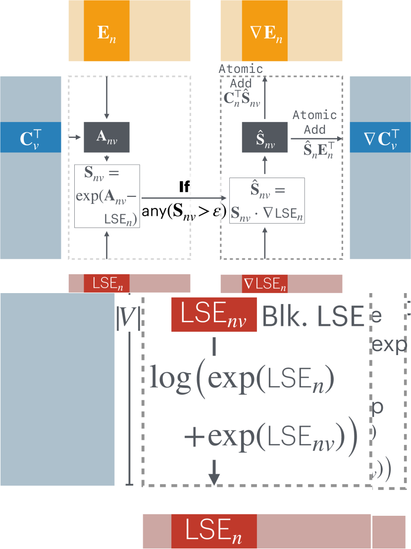
(a) Indexed matmul
(forward)

(b) Linear-log-sum-exp,
forward pass

(c) Linear-log-sum-exp,
backward pass

Figure 2: Access patterns and computation of blockwise (a) indexed matrix multiplication, (b) linear-log-sum-exp forward pass, and (c) linear-log-sum-exp backward pass. See Algorithms 1, 2 and 3 for the corresponding algorithms.

4.1 Memory-Efficient Indexed Matrix Multiplication

A naive computation of indexed matrix multiplication involves either explicit computation of the logits $\mathbf{{\color[rgb]{0.16015625,0.5,0.7265625}C}}^{\top}\mathbf{{\color[rgb]{0.953125,0.61328125,0.0703125}E}}$ with an $O(N|V|)$ memory cost, or indexing into the classifier $\mathbf{{\color[rgb]{0.16015625,0.5,0.7265625}C}}_{\mathbf{x}}=\left[{\color[rgb]{0.16015625,0.5,0.7265625}C}_{x_{1}}\ldots{\color[rgb]{0.16015625,0.5,0.7265625}C}_{x_{N}}\right]$ with an $O(ND)$ memory cost. Our implementation fuses the classifier indexing $\mathbf{{\color[rgb]{0.16015625,0.5,0.7265625}C}}_{\mathbf{x}}$ with the consecutive dot product between columns ${\color[rgb]{0.16015625,0.5,0.7265625}C}_{x_{i}}$ and ${\color[rgb]{0.953125,0.61328125,0.0703125}E}_{i}$ in a single CUDA/Triton kernel (Tillet et al., 2019). Our kernel retrieves the value $x_{i}$, the $x_{i}$-th column from $\mathbf{{\color[rgb]{0.16015625,0.5,0.7265625}C}}$, and the $i$-th column from $\mathbf{{\color[rgb]{0.953125,0.61328125,0.0703125}E}}$, and stores them in on-chip shared memory (SRAM). It then performs a dot product between ${\color[rgb]{0.16015625,0.5,0.7265625}C}_{x_{i}}$ and ${\color[rgb]{0.953125,0.61328125,0.0703125}E}_{i}$ and writes the result into global memory. The kernel uses only on-chip SRAM throughout and does not allocate any GPU memory. For efficiency, we perform all operations blockwise to make the best use of GPU cache structure. Algorithm 1 and Fig. 2(a) summarize the computation and access patterns.

Inputs:	$\mathbf{{\color[rgb]{0.953125,0.61328125,0.0703125}E}}\in\mathbb{R}^{{D}\times{N}}$, $\mathbf{{\color[rgb]{0.16015625,0.5,0.7265625}C}}\in\mathbb{R}^{{D}\times{|V|}}$, $\mathbf{x}\in\mathbb{R}^{N}$.
	Block sizes ${N_{B}}$ and ${D_{B}}$.
Outputs:	$\mathbf{o}=(\mathbf{{\color[rgb]{0.16015625,0.5,0.7265625}C}}^{\top}\mathbf{{\color[rgb]{0.953125,0.61328125,0.0703125}E}})_{\mathbf{x}}\in\mathbb{R}^{N}$

 

blocks $\mathbf{{\color[rgb]{0.953125,0.61328125,0.0703125}E}}_{n}$, $\mathbf{x}_{n}$$\triangleright$ Divide $\mathbf{{\color[rgb]{0.953125,0.61328125,0.0703125}E}}$ and $\mathbf{x}$ into blocks of size ${{D}\times{{N_{B}}}}$ and ${N_{B}}$, respectively

$\mathbf{o}_{n}=\mathbf{0}_{N_{B}}$$\triangleright$ Zero vector of size ${N_{B}}$ in on-chip SRAM blocks $\mathbf{{\color[rgb]{0.953125,0.61328125,0.0703125}E}}_{n,d}$$\triangleright$ Divide $\mathbf{{\color[rgb]{0.953125,0.61328125,0.0703125}E}}_{n}$ into blocks of size ${{{D_{B}}}\times{{N_{B}}}}$

$\mathbf{c}=\mathbf{{\color[rgb]{0.16015625,0.5,0.7265625}C}}_{\mathbf{x}_{n},d}$ $\triangleright$ Indexed load into on-chip SRAM

$\mathbf{o}_{n}\mathrel{+}=\mathbf{{\color[rgb]{0.953125,0.61328125,0.0703125}E}}_{n,d}\cdot\mathbf{c}$ $\triangleright$ Column-wide dot product

write $\mathbf{o}_{n}$$\triangleright$ From on-chip SRAM to main GPU memory

Algorithm 1 Memory-efficient indexed matrix multiplication

It is possible to compute the backward pass using a similar kernel. We found it to be easier and more memory-efficient to merge the backward implementation with the backward pass of the linear-log-sum-exp operator. The two operations share much of the computation and memory access pattern.

4.2 Memory-efficient Linear-log-sum-exp, Forward Pass

Implementing a serial memory-efficient linear-log-sum-exp is fairly straightforward: use a triple for-loop. The innermost loop computes the dot product between ${\color[rgb]{0.16015625,0.5,0.7265625}C}_{i}$ and ${\color[rgb]{0.953125,0.61328125,0.0703125}E}_{n}$ for the $i$-th token and the $n$-th batch element. The middle loop iterates over the vocabulary, updating the log-sum-exp along the way. Finally, the outermost loop iterates over all batch elements. Parallelizing over the outermost loop is trivial and would expose enough work to saturate the CPU due to the number of tokens in training batches (commonly in the thousands). Parallelization that exposes enough work to saturate the GPU is more challenging.

Let us first examine how efficient matrix multiplication between the batch of model output embeddings $\mathbf{{\color[rgb]{0.953125,0.61328125,0.0703125}E}}\in\mathbb{R}^{{D}\times{N}}$ and the classifier $\mathbf{{\color[rgb]{0.16015625,0.5,0.7265625}C}}\in\mathbb{R}^{{D}\times{|V|}}$ is implemented on modern GPUs (Kerr et al., 2017). A common method is to first divide the output $\mathbf{O}=\mathbf{{\color[rgb]{0.16015625,0.5,0.7265625}C}}^{\top}\mathbf{{\color[rgb]{0.953125,0.61328125,0.0703125}E}}\in\mathbb{R}^{{|V|}\times{N}}$ into a set of blocks of size ${{{M_{B}}}\times{{N_{B}}}}$. Independent CUDA blocks retrieve the corresponding parts $\mathbf{{\color[rgb]{0.953125,0.61328125,0.0703125}E}}_{n}$ of $\mathbf{{\color[rgb]{0.953125,0.61328125,0.0703125}E}}$ with size ${{D}\times{{N_{B}}}}$ and blocks $\mathbf{{\color[rgb]{0.16015625,0.5,0.7265625}C}}_{m}$ of $\mathbf{{\color[rgb]{0.16015625,0.5,0.7265625}C}}$ with size ${{D}\times{{M_{B}}}}$, and perform the inner product $\mathbf{O}_{nm}=\mathbf{{\color[rgb]{0.16015625,0.5,0.7265625}C}}_{m}^{\top}\mathbf{{\color[rgb]{0.953125,0.61328125,0.0703125}E}}_{n}$ along the $D$ dimension. Due to limited on-chip SRAM, most implementations use a for-loop for large values of $D$. They loop over smaller size ${{{D_{B}}}\times{{N_{B}}}}$ and ${{{D_{B}}}\times{{M_{B}}}}$ blocks and accumulate $\mathbf{O}_{nm}=\sum_{d}\mathbf{{\color[rgb]{0.16015625,0.5,0.7265625}C}}_{md}^{\top}\mathbf{{\color[rgb]{0.953125,0.61328125,0.0703125}E}}_{nd}$ in SRAM. Each CUDA block then writes $\mathbf{O}_{nm}$ back into global memory. This method exposes enough work to the GPU and makes efficient use of SRAM and L2 cache.

To produce $\textrm{log-sum-exp}(\mathbf{{\color[rgb]{0.16015625,0.5,0.7265625}C}}^{\top}\mathbf{{\color[rgb]{0.953125,0.61328125,0.0703125}E}})$, we use the same blocking and parallelization strategy as matrix multiplication. Each block first computes a matrix multiplication, then the log-sum-exp along the vocabulary dimension $m$ for its block, and finally updates $\mathbf{\mathrm{\color[rgb]{0.75390625,0.22265625,0.16796875}LSE}}$ with its result.

Note that multiple CUDA blocks are now all writing to the same location of $\mathbf{\mathrm{\color[rgb]{0.75390625,0.22265625,0.16796875}LSE}}$. This includes blocks in the same input range $n$ but different vocabulary ranges $m$. We use a spin-lock on an atomic operation in global memory to synchronize the updates by different CUDA blocks as this is simple to implement in our Triton framework and incurs little overhead. Alternative methods, such as an atomic compare-and-swap loop, may perform better when implementing in CUDA directly.

Algorithm 2 and Fig. 2(b) summarize the computation and access patterns.

Inputs:	$\mathbf{{\color[rgb]{0.953125,0.61328125,0.0703125}E}}\in\mathbb{R}^{{D}\times{N}}$ and $\mathbf{{\color[rgb]{0.16015625,0.5,0.7265625}C}}\in\mathbb{R}^{{D}\times{|V|}}$.
	Block sizes ${N_{B}}$, ${M_{B}}$, and ${D_{B}}$.
Outputs:	$\mathbf{\mathrm{\color[rgb]{0.75390625,0.22265625,0.16796875}LSE}}=\log\sum_{j}\exp({\color[rgb]{0.16015625,0.5,0.7265625}C}^{\top}_{j}\mathbf{{\color[rgb]{0.953125,0.61328125,0.0703125}E}})\in\mathbb{R}^{N}$

 

$\mathbf{\mathrm{\color[rgb]{0.75390625,0.22265625,0.16796875}LSE}}=-\mathbf{\infty}_{N}$$\triangleright$ $-\infty$ vector of size $N$ in main GPU memory all pairs of blocks $\mathbf{{\color[rgb]{0.953125,0.61328125,0.0703125}E}}_{n}$, $\mathbf{{\color[rgb]{0.16015625,0.5,0.7265625}C}}_{m}$$\triangleright$ Divide $\mathbf{{\color[rgb]{0.953125,0.61328125,0.0703125}E}}$ and $\mathbf{{\color[rgb]{0.16015625,0.5,0.7265625}C}}$ into blocks of size ${{D}\times{{N_{B}}}}$ and ${{D}\times{{M_{B}}}}$

$\mathbf{A}_{nm}=\mathbf{0}_{{{M_{B}}}\times{{N_{B}}}}$$\triangleright$ Zero matrix of size ${{{M_{B}}}\times{{N_{B}}}}$ in on-chip SRAM blocks $\mathbf{{\color[rgb]{0.953125,0.61328125,0.0703125}E}}_{n,d}$, $\mathbf{{\color[rgb]{0.16015625,0.5,0.7265625}C}}_{m,d}$$\triangleright$ Divide $\mathbf{{\color[rgb]{0.953125,0.61328125,0.0703125}E}}_{n}$ and $\mathbf{{\color[rgb]{0.16015625,0.5,0.7265625}C}}_{m}$ into blocks of ${{{D_{B}}}\times{{N_{B}}}}$ and ${{{D_{B}}}\times{{M_{B}}}}$

$\mathbf{A}_{nm}\mathrel{+}=\mathbf{{\color[rgb]{0.16015625,0.5,0.7265625}C}}_{m,d}^{\top}\cdot\mathbf{{\color[rgb]{0.953125,0.61328125,0.0703125}E}}_{n,d}$ $\triangleright$ Blockwise matrix multiplication

$\mathbf{\mathrm{\color[rgb]{0.75390625,0.22265625,0.16796875}LSE}}_{nm}=\log\sum\exp(\mathbf{A}_{nm}^{\top})$ $\triangleright$ Numerically stable implementation with max

$\mathbf{\mathrm{\color[rgb]{0.75390625,0.22265625,0.16796875}LSE}}_{n}=\log(\exp(\mathbf{\mathrm{\color[rgb]{0.75390625,0.22265625,0.16796875}LSE}}_{n})+\exp(\mathbf{\mathrm{\color[rgb]{0.75390625,0.22265625,0.16796875}LSE}}_{nm}))$$\triangleright$ Locking thread-safe log-add-exp

Algorithm 2 Memory-efficient linear-log-sum-exp, forward pass

4.3 Memory-efficient Linear-log-sum-exp, Backward Pass

The backward pass needs to efficiently compute two gradient updates:

$$\nabla\mathbf{{\color[rgb]{0.953125,0.61328125,0.0703125}E}}^{\top}=\mathbf{\lambda}^{\top}\frac{\partial}{\partial\mathbf{{\color[rgb]{0.953125,0.61328125,0.0703125}E}}}\log\sum\exp(\mathbf{{\color[rgb]{0.16015625,0.5,0.7265625}C}}^{\top}\mathbf{{\color[rgb]{0.953125,0.61328125,0.0703125}E}})\quad\text{and}\quad\nabla\mathbf{{\color[rgb]{0.16015625,0.5,0.7265625}C}}^{\top}=\lambda^{\top}\frac{\partial}{\partial\mathbf{{\color[rgb]{0.16015625,0.5,0.7265625}C}}}\log\sum\exp(\mathbf{{\color[rgb]{0.16015625,0.5,0.7265625}C}}^{\top}\mathbf{{\color[rgb]{0.953125,0.61328125,0.0703125}E}})$$

for a backpropagated gradient $\mathbf{\lambda}=\nabla\mathbf{\mathrm{\color[rgb]{0.75390625,0.22265625,0.16796875}LSE}}$. Formally, the gradient is defined as

$$\nabla\mathbf{{\color[rgb]{0.953125,0.61328125,0.0703125}E}}=\left(\mathbf{S}\cdot\nabla\mathbf{\mathrm{\color[rgb]{0.75390625,0.22265625,0.16796875}LSE}}\right)\mathbf{{\color[rgb]{0.16015625,0.5,0.7265625}C}}\quad\text{and}\quad\nabla\mathbf{{\color[rgb]{0.16015625,0.5,0.7265625}C}}=\left(\mathbf{S}\cdot\nabla\mathbf{\mathrm{\color[rgb]{0.75390625,0.22265625,0.16796875}LSE}}\right)^{\top}\mathbf{{\color[rgb]{0.953125,0.61328125,0.0703125}E}}$$

where $\mathbf{S}=\mathrm{softmax}(\mathbf{{\color[rgb]{0.16015625,0.5,0.7265625}C}}^{\top}\mathbf{{\color[rgb]{0.953125,0.61328125,0.0703125}E}})$ and $\cdot$ refers to the row-by-row elementwise multiplication of the softmax $\mathbf{S}$ and the gradient $\nabla\mathbf{\mathrm{\color[rgb]{0.75390625,0.22265625,0.16796875}LSE}}$: $\hat{\mathbf{S}}=\mathbf{S}\cdot\nabla\mathbf{\mathrm{\color[rgb]{0.75390625,0.22265625,0.16796875}LSE}}$.

Computationally, the backward pass is a double matrix multiplication $\mathbf{{\color[rgb]{0.16015625,0.5,0.7265625}C}}^{\top}\mathbf{{\color[rgb]{0.953125,0.61328125,0.0703125}E}}$ and $\hat{\mathbf{S}}\mathbf{{\color[rgb]{0.16015625,0.5,0.7265625}C}}$ or $\hat{\mathbf{S}}^{\top}\mathbf{{\color[rgb]{0.953125,0.61328125,0.0703125}E}}$ with intermediate matrices $\mathbf{S}$ and $\hat{\mathbf{S}}$ that do not fit into GPU memory and undergo a non-linear operation. We take a similar approach to the forward pass, recomputing the matrix $\mathbf{{\color[rgb]{0.16015625,0.5,0.7265625}C}}^{\top}\mathbf{{\color[rgb]{0.953125,0.61328125,0.0703125}E}}$ implicitly in the GPU’s shared memory. For the backward pass, we do not need to compute the normalization constant of the softmax, since $\mathbf{S}=\mathrm{softmax}(\mathbf{{\color[rgb]{0.16015625,0.5,0.7265625}C}}^{\top}\mathbf{{\color[rgb]{0.953125,0.61328125,0.0703125}E}})=\exp(\mathbf{{\color[rgb]{0.16015625,0.5,0.7265625}C}}^{\top}\mathbf{{\color[rgb]{0.953125,0.61328125,0.0703125}E}}-\mathbf{\mathrm{\color[rgb]{0.75390625,0.22265625,0.16796875}LSE}})$. This allows us to reuse the global synchronization of the forward pass, and compute $\mathbf{S}$ efficiently in parallel.

We implement the second matrix multiplication in the main memory of the GPU, as a blockwise implementation would require storing or synchronizing $\mathbf{S}$. Algorithm 3 and Fig. 2(c) summarize the computation and access patterns. A naive implementation of this algorithm requires zero additional memory but is slow due to repeated global memory load and store operations. We use two techniques to improve the memory access pattern: gradient filtering and vocabulary sorting.

Gradient filtering. By definition, the softmax $\mathbf{S}$ sums to one over the vocabulary dimension. If stored in bfloat16 with a 7-bit fraction, any value below $\varepsilon=2^{-12}$ will likely be ignored due to truncation in the summation or rounding in the normalization. This has profound implications for the softmax matrix $\mathbf{S}$: For any column, at most $\frac{1}{\varepsilon}=4096$ entries have non-trivial values and contribute to the gradient computation. All other values are either rounded to zero or truncated. In practice, the sparsity of the softmax matrix $\mathbf{S}$ is much higher: empirically, in frontier models we evaluate, less than $0.02\%$ of elements are non-zero. Furthermore, the sparsity of the softmax matrix grows as vocabulary size increases. In Algorithm 3, we take advantage of this sparsity and skip gradient computation for any block whose corresponding softmax matrix $S_{nm}$ has only negligible elements. We chose the threshold $\varepsilon=2^{-12}$ to be the smallest bfloat16 value that is not truncated. In practice, this leads to a 3.5x speedup without loss of precision in any gradient computation. See Section 5 for a detailed analysis.

The efficiency of gradient filtering is directly related to the block-level sparsity of the softmax matrix. We cannot control the overall sparsity pattern without changing the output. However, we can change the order of the vocabulary to create denser local blocks for more common tokens.

Inputs:	$\mathbf{{\color[rgb]{0.953125,0.61328125,0.0703125}E}}\in\mathbb{R}^{{D}\times{N}}$, $\mathbf{{\color[rgb]{0.16015625,0.5,0.7265625}C}}\in\mathbb{R}^{{D}\times{|V|}}$, $\mathbf{\mathrm{\color[rgb]{0.75390625,0.22265625,0.16796875}LSE}}\in\mathbb{R}^{N}$, and $\nabla\mathbf{\mathrm{\color[rgb]{0.75390625,0.22265625,0.16796875}LSE}}\in\mathbb{R}^{N}$.
	Block sizes ${N_{B}}$, ${M_{B}}$, and ${D_{B}}$.
	Accuracy threshold $\varepsilon$.
Outputs:	$\nabla\mathbf{{\color[rgb]{0.953125,0.61328125,0.0703125}E}}\in\mathbb{R}^{{D}\times{N}}$, $\nabla\mathbf{{\color[rgb]{0.16015625,0.5,0.7265625}C}}\in\mathbb{R}^{{D}\times{|V|}}$

 

all pairs of blocks $\mathbf{{\color[rgb]{0.953125,0.61328125,0.0703125}E}}_{n}$, $\mathbf{{\color[rgb]{0.16015625,0.5,0.7265625}C}}_{m}$$\triangleright$ Divide $\mathbf{{\color[rgb]{0.953125,0.61328125,0.0703125}E}}$ and $\mathbf{{\color[rgb]{0.16015625,0.5,0.7265625}C}}$ into blocks of size ${{D}\times{{N_{B}}}}$ and ${{D}\times{{M_{B}}}}$

$\mathbf{A}_{nm}=\mathbf{0}_{{{M_{B}}}\times{{N_{B}}}}$$\triangleright$ Zero matrix of size ${{{M_{B}}}\times{{N_{B}}}}$ in on-chip SRAM blocks $\mathbf{{\color[rgb]{0.953125,0.61328125,0.0703125}E}}_{n,d}$, $\mathbf{{\color[rgb]{0.16015625,0.5,0.7265625}C}}_{m,d}$$\triangleright$ Divide $\mathbf{{\color[rgb]{0.953125,0.61328125,0.0703125}E}}_{n}$ and $\mathbf{{\color[rgb]{0.16015625,0.5,0.7265625}C}}_{m}$ into blocks of ${{{D_{B}}}\times{{N_{B}}}}$ and ${{{D_{B}}}\times{{M_{B}}}}$

$\mathbf{A}_{nm}\mathrel{+}=\mathbf{{\color[rgb]{0.16015625,0.5,0.7265625}C}}_{m,d}^{\top}\cdot\mathbf{{\color[rgb]{0.953125,0.61328125,0.0703125}E}}_{n,d}$ $\triangleright$ Blockwise matrix multiplication

$\mathbf{S}_{nm}=\exp(\mathbf{A}_{nm}-\mathbf{\mathrm{\color[rgb]{0.75390625,0.22265625,0.16796875}LSE}}_{n})$ $\triangleright$ Compute the softmax all$(\mathbf{S}_{nm}<\varepsilon)$

skip $\triangleright$ Skip computation if below desired numerical precision blocks $\mathbf{{\color[rgb]{0.953125,0.61328125,0.0703125}E}}_{n,d}$, $\mathbf{{\color[rgb]{0.16015625,0.5,0.7265625}C}}_{m,d}$$\triangleright$ Divide $\mathbf{{\color[rgb]{0.953125,0.61328125,0.0703125}E}}_{n}$ and $\mathbf{{\color[rgb]{0.16015625,0.5,0.7265625}C}}_{m}$ into blocks of ${{{D_{B}}}\times{{N_{B}}}}$ and ${{{D_{B}}}\times{{M_{B}}}}$

$\nabla\mathbf{{\color[rgb]{0.953125,0.61328125,0.0703125}E}}^{\top}_{n,d}\mathrel{+}=\left(\mathbf{S}_{nm}\cdot\nabla\mathbf{\mathrm{\color[rgb]{0.75390625,0.22265625,0.16796875}LSE}}_{n}\right)\mathbf{{\color[rgb]{0.16015625,0.5,0.7265625}C}}_{m,d}$$\triangleright$ Locking thread-safe gradient update

$\nabla\mathbf{{\color[rgb]{0.16015625,0.5,0.7265625}C}}^{\top}_{m,d}\mathrel{+}=\left(\mathbf{S}_{nm}\cdot\nabla\mathbf{\mathrm{\color[rgb]{0.75390625,0.22265625,0.16796875}LSE}}_{n}\right)^{\top}\mathbf{{\color[rgb]{0.953125,0.61328125,0.0703125}E}}_{n,d}$$\triangleright$ Locking thread-safe gradient update

Algorithm 3 Memory-efficient linear-log-sum-exp, backward pass

Vocabulary sorting. Ideally the vocabulary would be ordered such that all tokens with non-trivial gradients would be contiguously located. This reduces the amount of computation wasted by partially populated blocks – ideally blocks would either be entirely empty (and thus skipped) or entirely populated. We heuristically group the non-trivial gradients by ordering the tokens by their average logit. Specifically, during the forward pass (described in Section 4.2) we compute the average logit per token using an atomic addition. For the backward pass, we divide the vocabulary dimension $|V|$ into blocks with similar average logit instead of arbitrarily. This requires a temporary buffer of size $O(|V|)$, about $1$ MB for the largest vocabularies in contemporary LLMs (Rivière et al., 2024).

Putting all the pieces together, we arrive at forward and backward implementations of cross-entropy that have negligible incremental memory footprint without sacrificing speed. Note that in practice, we compute the backward pass of the indexed matrix multiplication in combination with log-sum-exp (Algorithm 3). We subtract $1$ from the softmax $S_{i,x_{i}}$ for all ground-truth tokens $x_{1}\ldots x_{N}$.

5 Analysis

5.1 Runtime and Memory

First we examine the runtime and memory of various implementations of the cross-entropy loss $\log\mathrm{softmax}_{x_{i}}(\mathbf{{\color[rgb]{0.16015625,0.5,0.7265625}C}}^{\top}\mathbf{{\color[rgb]{0.953125,0.61328125,0.0703125}E}})$. We consider a batch of $8192$ tokens with a vocabulary size of $256000$ and hidden dimension $2304$. This corresponds to Gemma 2 (2B) (Rivière et al., 2024). We use the Alpaca dataset (Taori et al., 2023) for inputs and labels and Gemma 2 (2B) Instruct weights to compute $\mathbf{{\color[rgb]{0.953125,0.61328125,0.0703125}E}}$ and for $\mathbf{{\color[rgb]{0.16015625,0.5,0.7265625}C}}$. The analysis is summarized in Table 1. The baseline implements the loss directly in PyTorch (Paszke et al., 2019). This is the default in popular frameworks such as Torch Tune (Torch Tune Team, 2024) and Transformers (Wolf et al., 2019). This method has reasonable throughput but a peak memory usage of 28000MB of GPU memory to compute the loss+gradient (Table 1 row 5). Due to memory fragmentation, just computing the loss+gradient for the classifier head requires an 80GB GPU. torch.compile (Ansel et al., 2024) is able to reduce memory usage by 43% and computation time by 33%, demonstrating the effectiveness of kernel fusion (Table 1 row 4 vs. 5). Torch Tune (Torch Tune Team, 2024) includes a method to compute the cross-entropy loss that divides the computation into chunks and uses torch.compile to save memory. This reduces memory consumption by 65% vs. Baseline and by 40% vs. torch.compile (to 9631MB, see Table 1 row 3 vs. 4 and 5). Liger Kernels (Hsu et al., 2024) provide a memory-efficient implementation of the cross-entropy loss that, like Torch Tune, makes uses of chunked computation to reduce peak memory usage. While very effective at reducing the memory footprint, using 95% less memory than Baseline, it has a detrimental effect on latency, more than doubling the wall-clock time for the computation (Table 1, row 2 vs. 4). The memory usage of CCE grows with $O(N+|V|)$, as opposed to $O(N\times|V|)$ for Baseline, torch.compile, and Torch Tune, and $O(N\times D)$ for Liger Kernels. In practice, CCE has a negligible memory footprint regardless of vocabulary size or sequence length.

Compared to the fastest method, torch.compile, CCE computes the loss slightly faster (5%, 4ms, Table 1 row 1 vs. 4). This is because CCE does not write all the logits to global memory. CCE also computes the loss+gradient in slightly faster (6%, 8ms). This is because CCE is able to make use of the inherit sparsity of the gradient to skip computation.

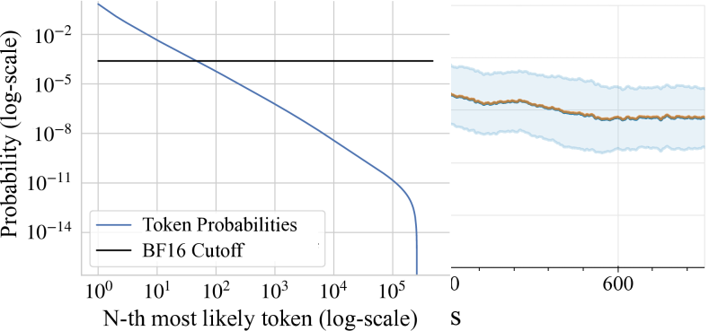
Figure 3: Average probability for the $i$th most likely token, log-log plot. The probabilities very quickly vanish below numerical precision.

The performance of CCE is enabled by both gradient filtering and vocabulary sorting. Without vocabulary sorting CCE takes 15% (23ms) longer (Table 1 row 1 vs. 6) and without gradient filtering it is 3.4x (356ms) longer (row 1 vs. 7). In Appendix A, we demonstrate that CCE (and other methods) can be made up to 3 times faster by removing tokens that are ignored from the loss computation.

In Appendix B we benchmark with more models. We find that as the ratio of vocabulary size ($|V|$) to hidden size ($D$) decreases, CCE begins to be overtaken in computation time for the Loss+Gradient, but continues to save a substantial amount of memory.

Loss

Gradient

Loss+Gradient

Method

Memory

Time

Memory

Time

Memory

Time

Lower bound

0.004MB

1161MB

1161MB

1) CCE (Ours)

1MB

43ms

1163MB

95ms

1164MB

135ms

2) Liger Kernels (Hsu et al., 2024)

1474MB

302ms

1474MB

303ms

3) Torch Tune Team (2024) (8 chunks)

8000MB

55ms

1630MB

115ms

9631MB

170ms

4) torch.compile

4000MB

49ms

12000MB

92ms

16000MB

143ms

5) Baseline

24000MB

82ms

16000MB

121ms

28000MB

207ms

6) CCE (No Vocab Sorting)

0.09MB

42ms

1162MB

104ms

1162MB

143ms

7) CCE (No Grad. Filter)

0.09MB

42ms

1162MB

324ms

1162MB

362ms

Table 1: Peak memory footprint and time to compute the loss, its gradient, and their combination. Note that intermediate buffers can often (but not always) be reused between the loss and gradient computation, resulting in lower peak memory consumption than the sum of the parts. Batch of $8192$ tokens with a vocabulary size of $256000$ and hidden dimension 2304. Embedding and classifier matrix taken during Gemma 2 (2B) training on Alpaca. Measured on an A100-SXM4 GPU with 80GB of RAM, PyTorch 2.4.1, CUDA 12.4, rounded to closest MB. Some numbers are multiples of $1000$ due to dimensions chosen and PyTorch’s allocation strategy. ‘Lower bound’ is the amount of memory required for the output buffer(s), i.e., $\nabla\mathbf{{\color[rgb]{0.953125,0.61328125,0.0703125}E}}$ and $\nabla\mathbf{{\color[rgb]{0.16015625,0.5,0.7265625}C}}$, this is the lower bound for the memory footprint of any method.

5.2 Gradient Filtering

Fig. 3 shows the sorted softmax probability of vocabulary entries. Note that the probabilities vanish very quickly and, for the top $10^{5}$ most likely tokens, there is a linear relationship between $\log\textrm{rank}$ and $\log\textrm{probability}$. Second, by the $\sim$50th most likely token, the probability has fallen bellow our threshold for gradient filtering.

This explains why we are able to filter so many values from the gradient computation without affecting the result. At these sparsity levels, most blocks of the softmax matrix $\mathbf{S}$ are empty.

(a) Gemma 2 2B

(b) Phi 3.5 Mini

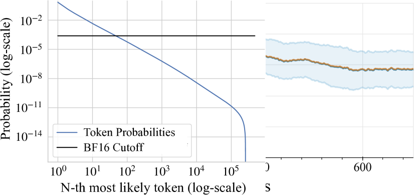
(c) Llama 3 8B

(d) Mistral Nemo

Figure 4: Training loss curves for four models on the Alpaca dataset (Taori et al., 2023). The loss curves for CCE and torch.compile are nearly indistinguishable, showing that the gradient filtering in CCE does not impair convergence. Results averaged over 5 seeds.

5.3 Training Stability

Fig. 4 demonstrates the training stability of CCE. We fine-tune Llama 3 8B Instruct (Dubey et al., 2024), Phi 3.5 Mini Instruct (Abdin et al., 2024), Gemma 2 2B Instruct (Rivière et al., 2024), and Mistral NeMo (Mistral AI Team, 2024) on the Alpaca Dataset (Taori et al., 2023) using CCE and torch.compile as the control. As shown in the figure, CCE and torch.compile have indistinguishable loss curves, demonstrating that the gradient filtering in CCE does not impair convergence.

6 Discussion

As vocabulary size $|V|$ has grown in language models, so has the memory footprint of the loss layer. The memory used by this one layer dominates the training-time memory footprint of many recent language models. We described CCE, an algorithm to compute $\ell_{i}=\log\mathrm{softmax}_{i}(C^{T}f(x_{1}\ldots x_{i-1}))$ and its gradient with negligible memory footprint.

Beyond the immediate impact on compact large-vocabulary LLMs, as illustrated in Fig. 1, we expect that CCE may prove beneficial for training very large models. Specifically, very large models are trained with techniques such as pipeline parallelism (Huang et al., 2019; Narayanan et al., 2019). Pipeline parallelism works best when all stages are equally balanced in computation load. Achieving this balance is easiest when all blocks in the network have similar memory-to-computation ratios. The classification head is currently an outlier, with a disproportionately high memory-to-computation ratio. CCE may enable better pipeline balancing or reducing the number of stages.

We implemented CCE using Triton (Tillet et al., 2019). Triton creates efficient GPU kernels and enables rapid experimentation but has some limitations in control flow. Specifically, the control flow must be specified at the block level and therefore our thread-safe log-add-exp and gradient filtering are constrained to operate at the block level as well. We expect that implementing CCE in CUDA may bring further performance gains because control flow could be performed at finer-grained levels.

It could also be interesting to extend CCE to other classification problems where the number of classes is large, such as image classification and contrastive learning.

Appendix A Removing Ignored Tokens

Loss

Gradient

Loss+Gradient

Method

Memory

Time

Memory

Time

Memory

Time

Lower bound

0.004MB

1161MB

1161MB

8) CCE (Ours)

1MB

15ms

1163MB

40ms

1164MB

52ms

9) Liger Kernels (Hsu et al., 2024)

1230MB

313ms

1228MB

315ms

10) Torch Tune Team (2024) (8 chunks)

2700MB

22ms

2709MB

52ms

5410MB

73ms

11) torch.compile

1356MB

18ms

4032MB

32ms

5388MB

50ms

12) Baseline

8076MB

28ms

5376MB

41ms

9420MB

70ms

13) CCE (No Vocab Sorting)

0.05MB

15ms

1162MB

46ms

1162MB

58ms

14) CCE (No Grad. Filter)

0.05MB

15ms

1162MB

156ms

1162MB

170ms

Table A1: Table 1 where all methods include a filter that removes tokens that are ignored in loss computation. This simple change represents large improvements in practice.

It is common to have tokens that have no loss computation when training LLMs in practice. Examples include padding, the system prompt, user input, etc.. While these tokens must be processed by the backbone – to enable efficient batching in the case of padding or to give the model the correct context for its prediction in the case of system prompts and use inputs – they do not contribute directly to the loss.

In all implementations we are aware of, the logits and loss for these ignored tokens is first computed and then set to zero. We notice that this is unnecessary. These tokens can be removed before logits+loss computation with no change to the loss/gradient and save a significant amount of computation.

Table A1 shows the performance of all methods in Table 1 with a filter that removes ignored tokens before logits+loss computation. This represents a significant speed up for all methods but Liger Kernels. Due to heavy chunking in Liger Kernels to save memory, it is bound by kernel launch overhead, not computation. Filtering ignored tokens is also a significant memory saving for most all but CCE (because CCE already uses the minimum amount of memory possible).

Appendix B Additional results

Table A2 shows additional results for Gemma 2 (9B), Gemma 2 (27B), and Llama 3 (Dubey et al., 2024), PHI 3.5 Mini (Abdin et al., 2024), and Mistral NeMo (Mistral AI Team, 2024) in the same setting as Table 1. For each model CCE is able to reduce the total memory consumed by the loss by an order of magnitude from the baseline. For forward (Loss) and backward (Gradient) passes combined, CCE is within 3MB of the lowest possible memory consumption. Compared to Gemma 2 (2B) all these models have a smaller ratio of the vocabulary size to hidden dimension. This has two impacts.

First, the number of tokens that have a significant gradient is largely constant (it is dependent on the data type). Therefore proportionally less of the gradient will be filtered out.

Second, for all other methods increasing the hidden dimension increase the amount of parallelism that can be achieved. Liger Kernels (Hsu et al., 2024) sets its chunk size based on $\nicefrac{{|V|}}{{D}}$ – the lower that ratio, the bigger the chunk size. As $\nicefrac{{|V|}}{{D}}$ continues to decrease, Liger Kernels is able to make better use of the GPU. All other methods use two matrix multiplications to compute the gradient. The amount of work that can be performed in parallel to compute $\nabla{\color[rgb]{0.953125,0.61328125,0.0703125}E}$ and $\nabla{\color[rgb]{0.16015625,0.5,0.7265625}C}$ is $B\times D$ and $|V|\times D$, respectively. The amount of parallel work for CCE is $B\times|V|$, thus increasing $D$ increases the amount of work but not the amount of parallelism. It may be possible leverage ideas from split-k matrix multiplication kernels to expose more parallelism to CCE for large values of $D$.

For the smallest $\nicefrac{{|V|}}{{D}}$ considered, Phi 3.5 Mini ($|V|$=$32064$, D=$3072$) ours is approximately $35\%$ slower (8ms) than torch.compile (although it uses substantially less memory). As this ratio grows, the relative performance of CCE increases.

		Loss				Gradient				Loss+Gradient
Method		Memory		Time		Memory		Time		Memory		Time
Gemma 2 (9B) (Rivière et al., 2024) ($|V|$=$256000$, D=$3584$)
Lower bound		0.004MB				1806MB				1806MB
CCE (Ours)		1MB		65ms		1808MB		140ms		1809MB		202ms
Liger Kernels (Hsu et al., 2024)		2119MB		419ms						2119MB		420ms
Torch Tune Team (2024) (8 chunks)		8000MB		75ms		3264MB		168ms		11264MB		243ms
torch.compile		4000MB		70ms		12000MB		133ms		16000MB		205ms
Baseline		24000MB		102ms		16000MB		164ms		28000MB		270ms
Gemma 2 (27B) (Rivière et al., 2024) ($|V|$=$256000$, D=$4608$)
Lower bound		0.004MB				2322MB				2322MB
CCE (Ours)		1MB		82ms		2324MB		194ms		2325MB		273ms
Liger Kernels (Hsu et al., 2024)		2948MB		365ms						2948MB		365ms
Torch Tune Team (2024) (8 chunks)		8000MB		93ms		4768MB		205ms		12768MB		297ms
torch.compile		4000MB		87ms		12000MB		168ms		16000MB		256ms
Baseline		24000MB		119ms		16000MB		197ms		28000MB		320ms
Llama 3 (8B) (Dubey et al., 2024) ($|V|$=$128256$, D=$4096$)
Lower bound		0.004MB				1066MB				1066MB
CCE (Ours)		0.6MB		36ms		1067MB		99ms		1068MB		131ms
Liger Kernels (Hsu et al., 2024)		1317MB		164ms						1317MB		164ms
Torch Tune Team (2024) (8 chunks)		2004MB		40ms		2521MB		91ms		4525MB		131ms
torch.compile		2004MB		39ms		6012MB		75ms		8016MB		114ms
Baseline		10020MB		49ms		8016MB		80ms		12024MB		131ms
Mistral NeMo (Mistral AI Team, 2024) ($|V|$=$131072$, D=$5120$)
Lower bound		0.004MB				1360MB				1360MB
CCE (Ours)		0.6MB		45ms		1361MB		126ms		1362MB		168ms
Liger Kernels (Hsu et al., 2024)		1872MB		167ms						1872MB		168ms
Torch Tune Team (2024) (8 chunks)		2048MB		49ms		3348MB		113ms		5396MB		162ms
torch.compile		2048MB		48ms		6144MB		94ms		8192MB		142ms
Baseline		10240MB		58ms		8192MB		99ms		12288MB		160ms
Phi 3.5 Mini (Abdin et al., 2024) ($|V|$=$32064$, D=$3072$)
Lower bound		0.004MB				236MB				236MB
CCE (Ours)		0.2MB		7ms		236MB		25ms		236MB		31ms
Liger Kernels (Hsu et al., 2024)		488MB		26ms						487MB		26ms
Torch Tune Team (2024) (8 chunks)		502MB		8ms		451MB		18ms		953MB		26ms
torch.compile		502MB		8ms		1504MB		15ms		2006MB		23ms
Baseline		2506MB		11ms		2004MB		16ms		3006MB		27ms

Table A2: Memory usage and time of CCE, Liger Kernels, Torch Tune, torch.compile, and Baseline for additional models. Batch of $8192$ tokens.

Appendix C Raw numbers for Fig. 1

Table A3 contains the raw numbers used to create Fig. 1. The maximum batch size for 16 GPUs was calculated by assuming that the total amount of memory available is $75\times 16$ (i.e., each 80GB GPU will be fully occupied expect for a 5GB buffer for various libraries), then subtracting the memory used for weights + optimizer + gradients and then diving by the memory used per token.

Model	Logits	Activations	Weights+Opt+Grad	Max Batch Size (Before)	Max Batch Size (After)	Increase
GPT 2	12564MB	1152MB	1045MB	$5866190$	$69845595$	$11.9$$\times$
GPT Neo (1.3B)	12564MB	6144MB	10421MB	$4268047$	$12996042$	$3.0$$\times$
GPT Neo (2.7B)	12564MB	10240MB	20740MB	$3471784$	$7731585$	$2.2$$\times$
Gemma (2B)	64000MB	4608MB	19121MB	$1155515$	$17204330$	$14.9$$\times$
Gemma 2 (27B)	64000MB	26496MB	207727MB	$739448$	$2525554$	$3.4$$\times$
Gemma 2 (2B)	64000MB	7488MB	19946MB	$1108206$	$10580057$	$9.5$$\times$
Llama 2 (13B)	8000MB	25600MB	99303MB	$2203057$	$2891512$	$1.3$$\times$
Llama 2 (7B)	8000MB	16384MB	51410MB	$3164429$	$4709560$	$1.5$$\times$
Llama 3 (70B)	32064MB	81920MB	538282MB	$397019$	$552414$	$1.4$$\times$
Llama 3 (8B)	32064MB	16384MB	61266MB	$1579333$	$4670136$	$3.0$$\times$
Mistral 7B	8000MB	16384MB	55250MB	$3154108$	$4694200$	$1.5$$\times$
Mixtral 8x7B	8000MB	16384MB	356314MB	$2344949$	$3489944$	$1.5$$\times$
Phi 1.5	12574MB	6144MB	10821MB	$4264482$	$12991781$	$3.0$$\times$
Phi 3 Medium	8003MB	25600MB	106508MB	$2188824$	$2873067$	$1.3$$\times$
Qwen 1.5 (7B)	37912MB	16384MB	58909MB	$1412087$	$4679564$	$3.3$$\times$

Table A3: Raw data for Fig. 1. Memory usage calculated using a global batch size of $65536$.

References

- Abdin et al. (2024) Marah I Abdin, Sam Ade Jacobs, Ammar Ahmad Awan, Jyoti Aneja, Ahmed Awadallah, Hany Awadalla, Nguyen Bach, Amit Bahree, Arash Bakhtiari, Harkirat S. Behl, et al. Phi-3 technical report: A highly capable language model locally on your phone, 2024. URL https://arxiv.org/abs/2404.14219.
- Ansel et al. (2024) Jason Ansel, Edward Z. Yang, Horace He, Natalia Gimelshein, Animesh Jain, Michael Voznesensky, Bin Bao, Peter Bell, David Berard, Evgeni Burovski, et al. Pytorch 2: Faster machine learning through dynamic python bytecode transformation and graph compilation. In ACM International Conference on Architectural Support for Programming Languages and Operating Systems, 2024.
- Chen et al. (2016) Tianqi Chen, Bing Xu, Chiyuan Zhang, and Carlos Guestrin. Training deep nets with sublinear memory cost, 2016. URL http://arxiv.org/abs/1604.06174.
- Chen et al. (2023) Yu-Hui Chen, Raman Sarokin, Juhyun Lee, Jiuqiang Tang, Chuo-Ling Chang, Andrei Kulik, and Matthias Grundmann. Speed is all you need: On-device acceleration of large diffusion models via GPU-aware optimizations. In Conference on Computer Vision and Pattern Recognition, Workshops, 2023.
- Choromanski et al. (2021) Krzysztof Marcin Choromanski, Valerii Likhosherstov, David Dohan, Xingyou Song, Andreea Gane, Tamás Sarlós, Peter Hawkins, Jared Quincy Davis, Afroz Mohiuddin, Lukasz Kaiser, David Benjamin Belanger, Lucy J. Colwell, and Adrian Weller. Rethinking attention with performers. In International Conference on Learning Representations, 2021.
- Dao et al. (2022) Tri Dao, Daniel Y. Fu, Stefano Ermon, Atri Rudra, and Christopher Ré. FlashAttention: Fast and memory-efficient exact attention with IO-awareness. In Neural Information Processing Systems, 2022.
- Dubey et al. (2024) Abhimanyu Dubey, Abhinav Jauhri, Abhinav Pandey, Abhishek Kadian, Ahmad Al-Dahle, Aiesha Letman, Akhil Mathur, Alan Schelten, Amy Yang, Angela Fan, et al. The Llama 3 herd of models, 2024. URL https://arxiv.org/abs/2407.21783.
- Gage (1994) Philip Gage. A new algorithm for data compression. The C Users Journal, 12(2):23–38, 1994.
- Goyal et al. (2017) Priya Goyal, Piotr Dollár, Ross B. Girshick, Pieter Noordhuis, Lukasz Wesolowski, Aapo Kyrola, Andrew Tulloch, Yangqing Jia, and Kaiming He. Accurate, large minibatch SGD: Training ImageNet in 1 hour, 2017. URL http://arxiv.org/abs/1706.02677.
- Grave et al. (2017) Edouard Grave, Armand Joulin, Moustapha Cissé, David Grangier, and Hervé Jégou. Efficient softmax approximation for gpus. In International Conference on Machine Learning, 2017.
- Gu & Dao (2023) Albert Gu and Tri Dao. Mamba: Linear-time sequence modeling with selective state spaces, 2023. URL https://arxiv.org/abs/2312.00752.
- Gu et al. (2022) Albert Gu, Karan Goel, and Christopher Ré. Efficiently modeling long sequences with structured state spaces. In International Conference on Learning Representations, 2022.
- Hillis & Steele (1986) W. Daniel Hillis and Guy L. Steele. Data parallel algorithms. Commun. ACM, 29(12):1170–1183, 1986.
- Hsu et al. (2024) Pin-Lun Hsu, Yun Dai, Vignesh Kothapalli, Qingquan Song, Shao Tang, and Siyu Zhu. Liger-Kernel: Efficient Triton kernels for LLM training, 2024. URL https://github.com/linkedin/Liger-Kernel.
- Huang et al. (2019) Yanping Huang, Youlong Cheng, Ankur Bapna, Orhan Firat, Dehao Chen, Mia Xu Chen, HyoukJoong Lee, Jiquan Ngiam, Quoc V. Le, Yonghui Wu, and Zhifeng Chen. GPipe: Efficient training of giant neural networks using pipeline parallelism. In Neural Information Processing Systems, 2019.
- Kerr et al. (2017) Andrew Kerr, Duane Merrill, Julien Demouth, and John Tran. CUTLASS: Fast linear algebra in CUDA C++, 2017. URL https://developer.nvidia.com/blog/cutlass-linear-algebra-cuda/.
- Kingma & Ba (2015) Diederik P. Kingma and Jimmy Ba. Adam: A method for stochastic optimization. In International Conference on Learning Representations, 2015.
- Kitaev et al. (2020) Nikita Kitaev, Lukasz Kaiser, and Anselm Levskaya. Reformer: The efficient transformer. In International Conference on Learning Representations, 2020.
- Kwon et al. (2023) Woosuk Kwon, Zhuohan Li, Siyuan Zhuang, Ying Sheng, Lianmin Zheng, Cody Hao Yu, Joseph Gonzalez, Hao Zhang, and Ion Stoica. Efficient memory management for large language model serving with pagedattention. In Symposium on Operating Systems Principles, 2023.
- Loshchilov & Hutter (2019) Ilya Loshchilov and Frank Hutter. Decoupled weight decay regularization. In International Conference on Learning Representations, 2019.
- Milakov & Gimelshein (2018) Maxim Milakov and Natalia Gimelshein. Online normalizer calculation for softmax, 2018. URL http://arxiv.org/abs/1805.02867.
- Mistral AI Team (2024) Mistral AI Team. Mistral NeMo, 2024. URL https://mistral.ai/news/mistral-nemo/.
- Narayanan et al. (2019) Deepak Narayanan, Aaron Harlap, Amar Phanishayee, Vivek Seshadri, Nikhil R. Devanur, Gregory R. Ganger, Phillip B. Gibbons, and Matei Zaharia. Pipedream: Generalized pipeline parallelism for DNN training. In ACM Symposium on Operating Systems Principles, 2019.
- Paszke et al. (2019) Adam Paszke, Sam Gross, Francisco Massa, Adam Lerer, James Bradbury, Gregory Chanan, Trevor Killeen, Zeming Lin, Natalia Gimelshein, Luca Antiga, et al. PyTorch: An imperative style, high-performance deep learning library. In Neural Information Processing Systems, 2019.
- Rabe & Staats (2021) Markus N. Rabe and Charles Staats. Self-attention does not need O(n) memory, 2021. URL https://arxiv.org/abs/2112.05682.
- Rajbhandari et al. (2020) Samyam Rajbhandari, Jeff Rasley, Olatunji Ruwase, and Yuxiong He. ZeRO: Memory optimizations toward training trillion parameter models. In International Conference for High Performance Computing, Networking, Storage and Analysis, 2020.
- Rivière et al. (2024) Morgane Rivière, Shreya Pathak, Pier Giuseppe Sessa, Cassidy Hardin, Surya Bhupatiraju, Léonard Hussenot, Thomas Mesnard, Bobak Shahriari, Alexandre Ramé, Johan Ferret, et al. Gemma 2: Improving open language models at a practical size, 2024. URL https://arxiv.org/abs/2408.00118.
- Tao et al. (2024) Chaofan Tao, Qian Liu, Longxu Dou, Niklas Muennighoff, Zhongwei Wan, Ping Luo, Min Lin, and Ngai Wong. Scaling laws with vocabulary: Larger models deserve larger vocabularies, 2024. URL https://arxiv.org/abs/2407.13623.
- Taori et al. (2023) Rohan Taori, Ishaan Gulrajani, Tianyi Zhang, Yann Dubois, Xuechen Li, Carlos Guestrin, Percy Liang, and Tatsunori B. Hashimoto. Stanford Alpaca: An instruction-following LLaMA model, 2023. URL https://github.com/tatsu-lab/stanford_alpaca.
- Tillet et al. (2019) Philippe Tillet, Hsiang-Tsung Kung, and David D. Cox. Triton: An intermediate language and compiler for tiled neural network computations. In ACM SIGPLAN International Workshop on Machine Learning and Programming Languages, 2019.
- Torch Tune Team (2024) Torch Tune Team. torchtune, 2024. URL https://github.com/pytorch/torchtune.
- Vaswani et al. (2017) Ashish Vaswani, Noam Shazeer, Niki Parmar, Jakob Uszkoreit, Llion Jones, Aidan N. Gomez, Lukasz Kaiser, and Illia Polosukhin. Attention is all you need. In Neural Information Processing Systems, 2017.
- Wang et al. (2020) Sinong Wang, Belinda Z. Li, Madian Khabsa, Han Fang, and Hao Ma. Linformer: Self-attention with linear complexity, 2020. URL https://arxiv.org/abs/2006.04768.
- Wolf et al. (2019) Thomas Wolf, Lysandre Debut, Victor Sanh, Julien Chaumond, Clement Delangue, Anthony Moi, Pierric Cistac, Tim Rault, Rémi Louf, Morgan Funtowicz, and Jamie Brew. Huggingface’s transformers: State-of-the-art natural language processing, 2019.
- Yu et al. (2023) Lili Yu, Daniel Simig, Colin Flaherty, Armen Aghajanyan, Luke Zettlemoyer, and Mike Lewis. MEGABYTE: Predicting million-byte sequences with multiscale transformers. In Neural Information Processing Systems, 2023.