Mixed-State Topological Order under Coherent Noises

Abstract

Mixed-state phases of matter under local decoherence have recently garnered significant attention due to the ubiquitous presence of noise in current quantum processors. One of the key issues is understanding how topological quantum memory is affected by realistic coherent noises, such as random rotation noise and amplitude damping noise. In this work, we investigate the intrinsic error threshold of the two-dimensional toric code, a paradigmatic topological quantum memory, under these coherent noises by employing both analytical and numerical methods based on the doubled Hilbert space formalism. A connection between the mixed-state phase of the decohered toric code and a non-Hermitian Ashkin-Teller-type statistical mechanics model is established, and the mixed-state phase diagrams under the coherent noises are obtained. We find remarkable stability of mixed-state topological order under random rotation noise with axes near the $Y$-axis of qubits. We also identify intriguing extended critical regions at the phase boundaries, highlighting a connection with non-Hermitian physics. The upper bounds for the intrinsic error threshold are determined by these phase boundaries, beyond which quantum error correction becomes impossible.

I Introduction

Topologically ordered phases of matter, which go beyond the conventional Landau paradigm, have been extensively investigated in the context of pure states [1, 2]. These quantum many-body states exhibit exotic properties such as long-range entanglement, robust ground-state degeneracy, and localized excitations with nontrivial exchange statistics. These features are resilient against local perturbations, making topological phases a promising platform for quantum error correction (QEC) and fault-tolerant quantum computing [3, 4]. The toric code, epitomizing $\mathbb{Z}_{2}$ topological order, serves as a prime example of a topological QEC code that can encode two logical qubits within its ground-state subspace [3].

Recently, significant progress has been made in realizing topologically ordered states on programmable quantum simulators [5, 6, 7, 8, 9, 10, 11]. However, the inevitable presence of noise in current noisy intermediate-scale quantum (NISQ) devices [12] renders the prepared quantum states as mixed states. Consequently, the mixed-state phase of matter has attracted considerable attention as a topic of both fundamental interest and practical importance [13, 14, 15, 16, 17, 18, 19, 20, 21, 22, 23, 24, 25, 26, 27, 28, 29, 30, 31, 32, 33, 34, 35, 36, 37, 38, 39, 40, 41, 42, 43, 44, 45, 46]. In particular, examining the mixed-state topological order can offer valuable insights into the intrinsic QEC properties of quantum memories under decoherence. For example, studies have shown that the toric code subject to incoherent bit-flip or phase-flip errors undergoes a mixed-state phase transition at a critical noise strength [17, 15, 16], which coincides with the error threshold of the toric code with the optimal decoder [4].

Previous studies on mixed-state topological order have mostly focused on incoherent local noises, where Pauli errors stochastically affect qubits. However, realistic quantum processors encounter coherent errors, which create a coherent superposition of different error states and give non-unique syndromes. Typical coherent errors include systematic unitary rotations caused by imperfect gate operations [47, 48, 49, 50] and amplitude damping due to spontaneous emission [51]. Therefore, it is crucial to study mixed-state topological order under coherent noises and understand their impact on quantum memories.

In this work, we address these questions by studying the two-dimensional (2D) toric code under two types of local coherent noises: (i) random rotation noise, where each qubit experiences unitary rotation around the $\vec{n}$ axis by an angle $\varphi_{e}$ according to some angle distribution $g(\varphi_{e})$, and (ii) amplitude damping noise with damping parameter $\gamma$ [see Fig. 1(a)]. We investigate the mixed-state phases of the decohered toric code under these noise models based on the doubled Hilbert space formalism [14, 15, 16]. We do so by mapping the Rényi-2 versions of information-theoretic quantities, such as anyon condensation/confinement parameters [15, 52, 53] and coherent information [54, 55], to observables in effective statistical mechanics (stat-mech) models. We show that these stat-mech models are the Ashkin-Teller-type models (with possibly anisotropic and imaginary coupling constants) for the considered coherent noises.

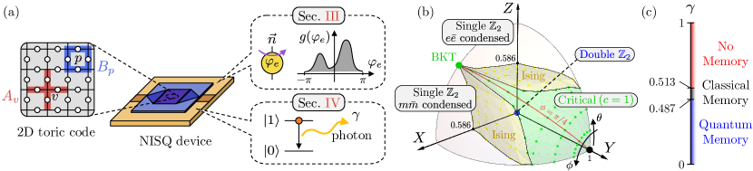
Figure 1: (a) Schematic of the coherent noise models under consideration. The two-dimensional toric code [see Eq. (1)] is subject to two types of coherent noises relevant to current noisy intermediate-scale quantum (NISQ) devices: (i) random rotation noise, where each qubit is rotated around the $\vec{n}$ axis by an angle $\varphi_{e}$ according to distribution $g(\varphi_{e})$ (see Sec. III), and (ii) amplitude damping noise, where each qubit decays to the ground state via spontaneous emission with probability $\gamma$ (see Sec. IV). (b) Phase diagram of the decohered toric code under random rotation noise. Radial direction and distance represent the rotation axis $\vec{n}$ and a parameter $R\in[0,1]$ that encodes information about the angle distribution $g(\varphi_{e})$ [see Eq. (12)], respectively. The system possesses quantum (classical) memory within (outside) the region enclosed by yellow and green phase boundaries. Two yellow boundaries belong to 2D Ising universality ($c=1/2$) and the green boundary with $R=1$ forms an extended critical region with $c=1$. A pure toric code is marked by the blue point located at the origin. (c) Phase diagram of the decohered toric code under amplitude damping noise. All phase diagrams illustrated here are based on the doubled Hilbert space formalism.

Specifically, we prove that the mixed-state phase of the decohered toric code under random rotation noise depends on the angle distribution $g(\varphi_{e})$ solely through a single parameter $R$ [defined in Eq. (12)]. With this simplification, we map the mixed-state phase diagram under random rotation noise for any rotation axis $\vec{n}$ and arbitrary distribution $g(\varphi_{e})$, using a combination of analytical results and tensor network simulations. Notably, we find that mixed-state topological order is highly resilient against random rotations with $\vec{n}$ near the $Y$-axis, where the phase boundary forms an extended critical region characterized by a central charge $c=1$. Additionally, we identify an intriguing two-dimensional phase boundary with Ising criticality, extended by the non-Hermitian nature of the effective stat-mech model. For amplitude damping noise, we discover two successive phase transitions as the damping rate $\gamma$ increases, first degrading the quantum memory to classical memory, and then to no memory. The mixed-state phase boundaries identified here establish upper bounds on the error threshold for coherent noises, within which QEC is feasible and beyond which QEC fails. The setup and the main results of this paper are illustrated in Fig. 1.

The rest of the paper is structured as follows. Sec. II briefly review the 2D toric code, the doubled Hilbert state formalism, and the considered information-theoretic diagnostics. Sec. III introduces random rotation noise and develops mapping to the stat-mech model. We discuss the general phase diagram and delineate the analytically tractable cases and the identified critical regions. Sec. IV presents the mixed-state phase diagram under the amplitude damping noise. Finally, we summarize our results and discuss open questions in Sec. V.

II Background

In this section, we provide a brief review of the 2D toric code and the doubled Hilbert space formalism. We then introduce two diagnostics used in subsequent sections to analyze mixed-state topological order under coherent noises: the anyon condensation/confinement parameters and the coherent information.

II.1 2D Toric Code

Consider an $L\times L$ square lattice with $N=2L^{2}$ qubits on its edges. The Hamiltonian of the 2D toric code (TC) defined on this lattice is given by [3]

$$H=-\sum_{v}A_{v}-\sum_{p}B_{p},$$ (1)

where $A_{v}=\prod_{e\in\partial v}X_{e}$ and $B_{p}=\prod_{e\in\partial p}Z_{e}$ are the star and plaquette operators, respectively [see Fig. 1(a)]. The vertices and edges of the lattice are denoted by $v$ and $e$, respectively, and ($X$, $Y$, $Z$) are the usual Pauli operators. Since $A_{v}$ and $B_{p}$ mutually commute, the ground states $|\Psi_{0}\rangle$ satisfy $A_{v}|\Psi_{0}\rangle=B_{p}|\Psi_{0}\rangle=|\Psi_{0}\rangle$ for all $v$ and $p$. On a torus, the ground-state subspace is fourfold degenerate, which can be utilized as a code space encoding two logical qubits.

We introduce an expression for TC ground states, which has been useful in studying TC under decoherence [29, 30]. Suppose that qubits are also placed on the vertices of the square lattice. The cluster state defined on this lattice is given by [56]

$$|\Psi_{c}\rangle\propto\prod_{e}(I+Z_{e}X_{v}X_{v^{\prime}})|\mathbf{z}_{v}=1,\mathbf{x}_{e}=1\rangle,$$ (2)

where $v$ and $v^{\prime}$ are vertices connected by edge $e=(v,v^{\prime})$, $|\mathbf{z}_{v}=1\rangle$ is a tensor product of the eigenstates of $Z_{v}$ operators with eigenvalue 1, and similarly for $|\mathbf{x}_{e}=1\rangle$. (The boldface indicates collective notation.) The TC ground state $|\Psi_{0}\rangle$ can be obtained from $|\Psi_{c}\rangle$ by performing forced measurements on vertex qubits [57]:

$$|\Psi_{0}\rangle\propto\langle\mathbf{z}_{v}=1|\Psi_{c}\rangle\propto\sum_{\mathbf{z}_{e},\mathbf{x}_{v}}\prod_{e}(1+z_{e}x_{v}x_{v^{\prime}})|\mathbf{z}_{e}\rangle.$$ (3)

II.2 Doubled Hilbert Space Formalism

Here, we review the doubled Hilbert space formalism [14, 15, 16], which views mixed states through the lens of pure states. For a density matrix $\rho$ defined on the Hilbert space $\mathcal{H}$, the Choi-Jamiołkowski (CJ) isomorphism maps $\rho$ to its Choi state $|\rho\rangle\!\rangle$, which is a pure state on the doubled Hilbert space $\mathcal{H}\otimes\bar{\mathcal{H}}$, where $\bar{\mathcal{H}}$ is a copy of $\mathcal{H}$ [58, 59]. More precisely, the (unnormalized) Choi state of $\rho=\sum_{i,j}\rho_{i,j}|i\rangle\langle j|$ is given by $|\rho\rangle\!\rangle=\sum_{i,j}\rho_{i,j}|i,\bar{j}\rangle\!\rangle$, where $|i,\bar{j}\rangle\!\rangle\equiv|i\rangle|\bar{j}\rangle$ and $\{|i\rangle\}$ is an orthonormal basis of $\mathcal{H}$. (The bar notation is for the copied Hilbert space.) A quantum channel $\mathcal{E}[\rho]=\sum_{a}K_{a}\rho K_{a}^{\dagger}$ with Kraus operators $\{K_{a}\}$ also maps under the CJ isomorphism into an operator $\mathbb{E}=\sum_{a}K_{a}\otimes\bar{K}_{a}^{*}$ acting on $\mathcal{H}\otimes\bar{\mathcal{H}}$.

For a pure TC state $\rho_{0}=|\Psi_{0}\rangle\langle\Psi_{0}|$, its Choi state is given by [see Eq. (3)]

$$|\rho_{0}\rangle\!\rangle\propto\sum_{\begin{subarray}{c}\mathbf{z}_{e},\bar{\mathbf{z}}_{e},\\ \mathbf{x}_{v},\bar{\mathbf{x}}_{v}\end{subarray}}\prod_{e}(1+z_{e}x_{v}x_{v^{\prime}})(1+\bar{z}_{e}\bar{x}_{v}\bar{x}_{v^{\prime}})|\mathbf{z}_{e},\bar{\mathbf{z}}_{e}\rangle\!\rangle,$$ (4)

which possesses double topological order, i.e., its topological quantum field theory is the product of two $\mathbb{Z}_{2}$ TC theories. Under local decoherence described by a channel $\mathcal{E}=\prod_{e}\mathcal{E}_{e}$, the density state becomes $\rho_{D}=\mathcal{E}[\rho_{0}]$ and its Choi state $|\rho_{D}\rangle\!\rangle=\mathbb{E}|\rho_{0}\rangle\!\rangle$ may lose the double topological order depending on the decoherence strength [15]. From $\mathrm{Tr}[\rho_{D}^{2}]=\langle\!\langle\rho_{D}|\rho_{D}\rangle\!\rangle=\langle\!\langle\rho_{0}|\mathbb{E}^{\dagger}\mathbb{E}|\rho_{0}\rangle\!\rangle$, the purity of the decohered TC can be written as [30]

$$\mathrm{Tr}[\rho_{D}^{2}]\propto\sum_{\mathbf{x}_{v},\bar{\mathbf{x}}_{v},\mathbf{t}_{v},\bar{\mathbf{t}}_{v}}\prod_{e}\omega_{e},$$ (5)

where

$$\omega_{e}\equiv\sum_{z_{e},\bar{z}_{e},z^{\prime}_{e},\bar{z}^{\prime}_{e}=\pm 1}\langle\!\langle z^{\prime}_{e},\bar{z}^{\prime}_{e}|\mathbb{E}_{e}^{\dagger}\mathbb{E}_{e}|z_{e},\bar{z}_{e}\rangle\!\rangle$$ (6)

$$\hskip 5.0pt\times(1+z_{e}x_{v}x_{v^{\prime}})(1+\bar{z}_{e}\bar{x}_{v}\bar{x}_{v^{\prime}})(1+z^{\prime}_{e}t_{v}t_{v^{\prime}})(1+\bar{z}^{\prime}_{e}\bar{t}_{v}\bar{t}_{v^{\prime}}).$$

The purity Eq. (5) can be interpreted as a partition function of a stat-mech model of Ising spins ($x_{v}$, $\bar{x}_{v}$, $t_{v}$, $\bar{t}_{v}$) on the vertices of the square lattice, with Eq. (6) being the local Boltzmann weight on edge $e$. Therefore, we can examine the change in double topological order under decoherence by studying the effective stat-mech model Eq. (5). In Sec. III and IV, we compute $\omega_{e}$ for coherent noises and determine the mixed-state phase diagram by examining the corresponding stat-mech model.

II.3 Diagnostics

Local quantum channels can always be purified to a finite-depth unitary circuit on an enlarged Hilbert space with ancillary qubits so that functions linear in density matrix (e.g., $\mathrm{Tr}[\rho_{D}O]$ for some observables $O$) are smooth in tuning parameters of the local channel [14, 16, 17]. Consequently, detecting phase transitions in mixed states decohered under local quantum channels requires considering functions nonlinear in density matrices, such as information-theoretic quantities. This section introduces two information-theoretic diagnostics that will be used throughout the paper.

II.3.1 Anyon Condensation/Confinement Parameters

Consider a density matrix $\rho_{0}^{\alpha\bar{\beta}}\equiv w_{\alpha}(l)\rho_{0}w_{\beta}^{\dagger}(l)$, where $w_{\alpha}(l)$ ($w_{\beta}(l)$) is a string operator creating a pair of $\alpha$ ($\beta$) anyons at the endpoints $i$ and $j$ of an open string $l$. Letting $\rho_{D}^{\alpha\bar{\beta}}\equiv\mathcal{E}[\rho_{0}^{\alpha\bar{\beta}}]$, the $\alpha\bar{\beta}$ anyon condensation and confinement parameters are defined as follows [15, 52, 53]:

$$\langle\!\langle I\bar{I}|\alpha\bar{\beta}\rangle\!\rangle \equiv\lim_{|i-j|\rightarrow\infty}\frac{\langle\!\langle\rho_{D}|\rho_{D}^{\alpha\bar{\beta}}\rangle\!\rangle}{\langle\!\langle\rho_{D}|\rho_{D}\rangle\!\rangle},$$ (7)

$$\langle\!\langle\alpha\bar{\beta}|\alpha\bar{\beta}\rangle\!\rangle \equiv\lim_{|i-j|\rightarrow\infty}\frac{\langle\!\langle\rho_{D}^{\alpha\bar{\beta}}|\rho_{D}^{\alpha\bar{\beta}}\rangle\!\rangle}{\langle\!\langle\rho_{D}|\rho_{D}\rangle\!\rangle}.$$

The condensation parameter $\langle\!\langle I\bar{I}|\alpha\bar{\beta}\rangle\!\rangle$ takes a nonzero finite constant value when $\alpha\bar{\beta}$ anyons are condensed, suggesting that $\rho_{0}^{\alpha\bar{\beta}}$ indistinguishable from the ground state $\rho_{0}$ under decoherence. It vanishes when $\alpha\bar{\beta}$ anyons are not condensed. Meanwhile, the confinement parameter $\langle\!\langle\alpha\bar{\beta}|\alpha\bar{\beta}\rangle\!\rangle$ vanishes when $\alpha\bar{\beta}$ anyons are confined, indicating that $|\rho_{D}^{\alpha\bar{\beta}}\rangle\!\rangle$ is not a physically normalizable state. It attains a nonzero finite value when $\alpha\bar{\beta}$ anyons are deconfined. Note that condensing one anyon confines all other anyons with nontrivial mutual statistics, following the standard anyon condensation rule [60, 61].

On a related note, the distinguishability between density matrices $\rho$ and $\sigma$ can be measured by the quantum relative entropy $D(\rho\|\sigma)\equiv\mathrm{Tr}[\rho(\log\rho-\log\sigma)]$ [62], which diverges when $\rho$ and $\sigma$ are orthogonal and takes a finite value otherwise. A useful related quantity is the Rényi relative entropy [63]:

$$D^{(n)}(\rho\|\sigma)\equiv\frac{1}{1-n}\log\left(\frac{\mathrm{Tr}[\rho\sigma^{n-1}]}{\mathrm{Tr}[\rho^{n}]}\right),$$ (8)

which recovers $D(\rho\|\sigma)$ as $n\rightarrow 1$. The anyon condensation parameters are related to the Rényi-2 relative entropy as $D^{(2)}(\rho_{D}\|\rho_{D}^{\alpha\bar{\beta}})=-\log\langle\!\langle I\bar{I}|\alpha\bar{\beta}\rangle\!\rangle$. Thus, when $\alpha\bar{\beta}$ anyons are condensed (not condensed), $D^{(2)}(\rho_{D}\|\rho_{D}^{\alpha,\bar{\beta}})$ becomes finite (infinite), indicating that $\rho_{D}$ and $\rho_{D}^{\alpha,\bar{\beta}}$ are indistinguishable (orthogonal).

The anyon parameters in Eq. (7) for the decohered TC can be represented as observables in the stat-mech model Eq. (5) as follows [30]:

$$\langle\!\langle I\bar{I}|e\bar{e}\rangle\!\rangle =\lim_{|i-j|\rightarrow\infty}\langle x_{i}\bar{x}_{i}x_{j}\bar{x}_{j}\rangle,$$ (9)

$$\langle\!\langle e\bar{I}|e\bar{I}\rangle\!\rangle =\lim_{|i-j|\rightarrow\infty}\langle x_{i}t_{i}x_{j}t_{j}\rangle,$$

$$\langle\!\langle I\bar{I}|m\bar{m}\rangle\!\rangle =\lim_{|\tilde{i}-\tilde{j}|\rightarrow\infty}\langle\mu_{\tilde{i}}^{x}\mu_{\tilde{i}}^{\bar{x}}\mu_{\tilde{j}}^{x}\mu_{\tilde{j}}^{\bar{x}}\rangle,$$

$$\langle\!\langle m\bar{I}|m\bar{I}\rangle\!\rangle =\lim_{|\tilde{i}-\tilde{j}|\rightarrow\infty}\langle\mu_{\tilde{i}}^{x}\mu_{\tilde{i}}^{t}\mu_{\tilde{j}}^{x}\mu_{\tilde{j}}^{t}\rangle,$$

where $i$ and $j$ ($\tilde{i}$ and $\tilde{j}$) are the endpoints of the string defined on the original (dual) lattice. Here, $\mu^{y}$ (with $y=x,\bar{x},t,\bar{t}$) is the disorder parameter of $y$ spins [64]. We review the derivation of the correspondence Eq. (9) in Appendix A.1.

II.3.2 Coherent Information

Let $Q$ represent the TC and $R$ be the two-qubit reference system that is maximally entangled with two logical qubits of the TC. To diagnose the amount of retrievable quantum information encoded in the TC after channel $\mathcal{E}$, one can consider the coherent information $I_{c}(R\rangle Q)\equiv S(\mathcal{E}[\rho_{Q}])-S(\mathcal{E}[\rho_{RQ}])$ [54, 55], where $S(\rho)=-\mathrm{Tr}[\rho\log\rho]$ is the von Neumann entropy. Without decoherence (i.e., $\mathcal{E}=I$), the TC achieves $I_{c}=2\log 2$, a condition necessary and sufficient for the existence of an exact QEC protocol. Since $I_{c}$ monotonically decreases under channel $\mathcal{E}$, the noise strength at which $I_{c}$ drops from $2\log 2$ provides an upper bound for the error threshold of any QEC scheme. Thus, investigating $I_{c}$ can reveal the extent to which encoded quantum information can persist under noise.

In practice, we consider the Rényi coherent information [17]:

$$I_{c}^{(n)}(R\rangle Q) \equiv S^{(n)}(\mathcal{E}[\rho_{Q}])-S^{(n)}(\mathcal{E}[\rho_{RQ}])$$ (10)

$$=\frac{1}{n-1}\log\left(\frac{\mathrm{Tr}[\mathcal{E}[\rho_{RQ}]^{n}]}{\mathrm{Tr}[\mathcal{E}[\rho_{Q}]^{n}]}\right),$$

where $S^{(n)}(\rho)=(1-n)^{-1}\log\mathrm{Tr}[\rho^{n}]$ is the $n$th Rényi entropy. As $n\rightarrow 1$, $I_{c}^{(n)}$ recovers $I_{c}$. In Appendix A.2, we derive the expression for $I_{c}^{(2)}$ in terms of the stat-mech model [see Eq. (34) and (36)]. Although $I_{c}^{(2)}$ does not give a rigorous error threshold of the code, it is relatively easy to compute and in many cases tracks the tendency of $I_{c}$. The error threshold obtained from $I_{c}^{(2)}$ provides an upper bound for the true error threshold corresponding to $I_{c}$, at which the decodability transition occurs.

III Random Rotation Noise

In this section, we study the decohered TC under random rotation noise. First, let’s clarify the terminology before introducing the model. We refer to noises where an operator $O$ is applied with probability $p$, like the bit-flip error $\rho\mapsto(1-p)\rho+pX\rho X$, as “stochastic $O$ noise.” By coherent noise, we mean noise that can produce a coherent superposition of different error states (with respect to Pauli syndrome measurements). Thus, stochastic noise is generally coherent, except for stochastic $X$, $Y$, and $Z$ noises, which are incoherent.

A random rotation noise is represented by a quantum channel $\mathcal{E}_{\mathrm{rot}}=\prod_{e}\mathcal{E}_{e}$, with

$$\mathcal{E}_{e}[\rho]\equiv\int_{\varphi_{e}}g(\varphi_{e})U_{e}(\varphi_{e})\rho U_{e}^{\dagger}(\varphi_{e}),$$ (11)

where $U_{e}(\varphi_{e})=e^{-i\varphi_{e}(\vec{n}\cdot\vec{\sigma})_{e}}$ and $\int_{\varphi_{e}}\equiv\int_{-\pi}^{\pi}d\varphi_{e}$. Here, each qubit is independently rotated around the axis $\vec{n}=(n_{x},n_{y},n_{z})$ by an angle $\varphi_{e}$ following a probability distribution $g(\varphi_{e})$ defined on $[-\pi,\pi)$ [see Fig. 1(a)]. Such noise often arises in current quantum processors due to imperfect gate operations [47, 48, 49, 50]. We are interested in $\rho_{D}=\mathcal{E}_{\mathrm{rot}}[\rho_{0}]$ and consider an arbitrary distribution function $g(\varphi_{e})$.

The random rotation noise Eq. (11) is in general coherent and not stochastic. However, Eq. (11) reduces to the stochastic $\vec{n}\cdot\vec{\sigma}$ noise with probability $p=\int_{\varphi_{e}}g(\varphi_{e})\sin^{2}\varphi_{e}$ for special cases with even angle distributions, i.e., $g(\varphi_{e})=g(-\varphi_{e})$ (see Appendix B.1 for a proof). Therefore, Eq. (11) includes previously studied incoherent Pauli noises, e.g., bit-flip and phase-flip noise, as special cases. See Fig. 2(a) for a summary of the properties of the random rotation noise according to its angle distribution $g(\varphi_{e})$ and rotation axis $\vec{n}$.

Since mixed-state phases of matter do not change under a finite-depth quantum channel [21, 22], the mean of the distribution $g(\varphi_{e})$ is unimportant because it can be set to zero via depth-1 global unitary rotation. This implies that a mixed state under an angle distribution symmetric about its mean is in the same phase as the mixed state under the corresponding stochastic noise [see Fig. 2(b)]. One may expect that an asymmetric distribution might lead to a new phase. However, we show below that it also leads to the same mixed-state phase as the symmetric distributions within the doubled Hilbert space formalism.

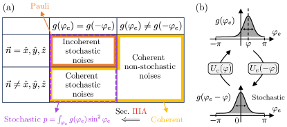
Figure 2: (a) Summary of the properties of the random rotation noise Eq. (11), based on its angle distribution $g(\varphi_{e})$ and rotation axis $\vec{n}$. Sec. III.1 shows that, within the doubled Hilbert space formalism, it is sufficient to study even distributions satisfying $g(\varphi_{e})=g(-\varphi_{e})$. (b) Since a distribution symmetric to its mean $\phi$ can be connected to an even distribution via a depth-1 unitary $U_{e}(\varphi)$, both distributions lead to the same mixed-state phase.

III.1 Mapping to Statistical Mechanics Model

Within the doubled Hilbert space formalism, we can study the mixed-state phase of the decohered TC under general angle distribution $g(\varphi_{e}$) by only considering the cases with $g(\varphi_{e})=g(-\varphi_{e})$. This simplification follows from the observation that the purity $\mathrm{Tr}[\rho_{D}]^{2}$ depends on $g(\varphi_{e})$ only through a single parameter

$$R\equiv 1-\left|\int_{\varphi_{e}}g(\varphi_{e})e^{2i\varphi_{e}}\right|^{2}.$$ (12)

Namely, all the information about $g(\varphi_{e})$ is encoded in $R$ (see Appendix B.2 for a proof). For example, we have $R=0$ for any global rotation with $g(\varphi_{e})=\delta(\varphi_{e}-\epsilon)$, and $R=1$ for maximally random noise with $g(\varphi_{e})=(2\pi)^{-1}$. The distributions with the same value of $R$ belong to the same mixed-state phase, and therefore we can focus on even distributions below. The phase diagram obtained from even distributions can be directly translated for general distributions by expressing $R$ in terms of parameters characterizing the distribution (see Sec. III.3).

Under the CJ isomorphism, the channel Eq. (11) is mapped to $\mathbb{E}_{\mathrm{rot}}=\prod_{e}\mathbb{E}_{e}$, where

$$\mathbb{E}_{e}=\int_{\varphi_{e}}g(\varphi_{e})e^{-i\varphi_{e}(\vec{n}\cdot\vec{\sigma})_{e}}\otimes\overline{e^{i\varphi_{e}(\vec{n}^{\prime}\cdot\vec{\sigma})_{e}}},$$ (13)

where $\vec{n}^{\prime}=(n_{x},-n_{y},n_{z})$ is introduced for the copied Hilbert space. By assuming even $g(\varphi_{e})$, we show in Appendix B.3 that the purity $\mathrm{Tr}[\rho_{D}^{2}]=\langle\!\langle\rho_{0}|\mathbb{E}_{\mathrm{rot}}^{\dagger}\mathbb{E}_{\mathrm{rot}}|\rho_{0}\rangle\!\rangle$ in the thermodynamic limit ($L\rightarrow\infty$) is proportional to the partition function $\sum_{\mathbf{s}_{v},\bm{\tau}_{v}}\prod_{e}\omega_{e}$ with

$$\omega_{e}\propto 1+J_{1}s_{v}s_{v^{\prime}}+J_{2}\tau_{v}\tau_{v^{\prime}}+Ks_{v}s_{v^{\prime}}\tau_{v}\tau_{v^{\prime}},$$ (14)

where $s_{v}\equiv x_{v}\bar{x}_{v}$ and $\tau_{v}\equiv\bar{x}_{v}t_{v}$ are the Ising spins residing on vertices of a square lattice, and

$$J_{1} =\frac{R(\sin^{2}\theta\cos^{2}\phi+\cos^{2}\theta)}{2-R+R\sin^{2}\theta\sin^{2}\phi},$$ (15)

$$J_{2} =\frac{R(\sin^{2}\theta\cos^{2}\phi-\cos^{2}\theta)}{2-R+R\sin^{2}\theta\sin^{2}\phi},$$

$$K =\frac{2-R-R\sin^{2}\theta\sin^{2}\phi}{2-R+R\sin^{2}\theta\sin^{2}\phi}.$$

Here, we parameterize the rotation axis as $\vec{n}=(\sin\theta\sin\phi,\cos\theta,\sin\theta\cos\phi)$, which is the spherical coordinates with the $Y$-axis as the polar axis [see Fig. 1(b)]. We can rewrite Eq. (14) as a local Boltzmann weight $\omega_{e}\propto e^{\mathcal{J}_{1}s_{v}s_{v^{\prime}}+\mathcal{J}_{2}\tau_{v}\tau_{v^{\prime}}+\mathcal{K}s_{v}s_{v^{\prime}}\tau_{v}\tau_{v^{\prime}}}$. The three coupling constants $\mathcal{J}_{1}$, $\mathcal{J}_{2}$, $\mathcal{K}$ are determined by $J_{1}$, $J_{2}$, $K$, and can generally be anisotropic and complex (see Appendix B.3 for details). In particular, the model gains its non-Hermiticity as the $y$-component of $\vec{n}$ increases. Consequently, $\mathrm{Tr}[\rho_{D}^{2}]$ is mapped to the partition function of the non-Hermitian anisotropic Ashkin-Teller (AT) model. This is one of our main results and we emphasize that this mapping can be leveraged to investigate decohered TC under random rotation noise with any rotation axis $\vec{n}$ and arbitrary angle distribution $g(\varphi_{e})$.

From Eq. (9), the anyon parameters can be read as

$$\langle\!\langle I\bar{I}|e\bar{e}\rangle\!\rangle =\lim_{|i-j|\rightarrow\infty}\langle s_{i}s_{j}\rangle,$$ (16)

$$\langle\!\langle e\bar{I}|e\bar{I}\rangle\!\rangle =\lim_{|i-j|\rightarrow\infty}\langle s_{i}\tau_{i}s_{j}\tau_{j}\rangle,$$

$$\langle\!\langle I\bar{I}|m\bar{m}\rangle\!\rangle =\lim_{|\tilde{i}-\tilde{j}|\rightarrow\infty}\langle\mu_{\tilde{i}}^{\tau}\mu_{\tilde{j}}^{\tau}\rangle,$$

$$\langle\!\langle m\bar{I}|m\bar{I}\rangle\!\rangle =\lim_{|\tilde{i}-\tilde{j}|\rightarrow\infty}\langle\mu_{\tilde{i}}^{s}\mu_{\tilde{i}}^{\tau}\mu_{\tilde{j}}^{s}\mu_{\tilde{j}}^{\tau}\rangle,$$

which are the correlation functions in the model Eq. (14). The stat-mech expression for the Rényi-2 coherent information is given by

$$I_{c}^{(2)}(R\rangle Q) =\log\left(\frac{\sum_{a,b=0,1}e^{-\Delta F_{s,\tau}^{(a,b)}}}{\sum_{a,b=0,1}e^{-\Delta F_{\tau,s\tau}^{(a,b)}}}\right),$$ (17)

where $\Delta F_{s,\tau}^{(a,b)}$ is a free energy cost of forming defects in the interactions $s_{v}s_{v^{\prime}}$ and $\tau_{v}\tau_{v^{\prime}}$ along the non-contractible loop pattern $(a,b)$, and similarly for $\Delta F_{\tau,s\tau}^{(a,b)}$ (see Appendix. A.2 for details). Using these two diagnostics, we can determine the phase of the model Eq. (14) (and hence that of $\rho_{D}$) and determine the fate of the quantum memory under random rotation noise.

III.2 General Phase Diagram

In the following, we numerically map out the general phase diagram of the stat-mech model Eq. (14) with respect to $(R,\phi,\theta)$. From the symmetry of Eq. (15), it suffices to study the parameter regime $0\leq R\leq 1$ and $0\leq\phi,\theta\leq\pi/2$. We represent the partition function of the stat-mech model into a tensor network and employ the corner transfer matrix renormalization group (CTMRG) algorithm [65, 66, 67] to approximately contract the tensor network. The phase boundaries are determined by pinpointing the parameters where the correlation length diverges and the order parameters change (see Fig. 3). The result is summarized in Fig. 1(b), where the phase boundaries are marked by yellow and green surfaces. We have confirmed that the correlation length $\xi_{D}$ increases as we increase the bond dimension $D$ of the corner tensors (not shown). The model has the following three phases:

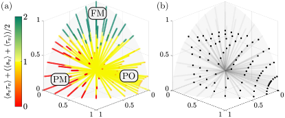
Figure 3: CTMRG results for the statistical mechanics model Eq. (14). (a) shows $\langle s_{v}\tau_{v}\rangle+(\langle s_{v}\rangle+\langle\tau_{v}\rangle)/2$, which takes the values close to 0, 1, and 2 for the paramagnetic (PM), partially ordered (PO), and ferromagnetic (FM) phases, respectively. (b) shows the points where the correlation length achieves the maximum value for each ray (gray lines). The bond dimension used is $D=40$.

1. Partially ordered (PO) phase = Quantum memory:
   In this case, $\langle s_{v}\tau_{v}\rangle\neq 0$ and $\langle s_{v}\rangle=\langle\tau_{v}\rangle=0$ so that $\langle\!\langle I\bar{I}|e\bar{e}\rangle\!\rangle=\langle\!\langle I\bar{I}|m\bar{m}\rangle\!\rangle=0$ and $\langle\!\langle e\bar{I}|e\bar{I}\rangle\!\rangle$, $\langle\!\langle m\bar{I}|m\bar{I}\rangle\!\rangle\neq 0$. Thus, the PO phase corresponds to double $\mathbb{Z}_{2}$ topological order and $\rho_{D}$ hosts quantum memory. Indeed, the pure TC with $R=0$ yields $\mathcal{J}_{1}=\mathcal{J}_{2}=0$ and $\mathcal{K}=\infty$, which belongs to the PO phase.

2. Ferromagnetic (FM) phase = Classical Memory:
   In this case, $\langle s_{v}\tau_{v}\rangle$, $\langle s_{v}\rangle$, $\langle\tau_{v}\rangle\neq 0$ so that $\langle\!\langle I\bar{I}|m\bar{m}\rangle\!\rangle=\langle\!\langle m\bar{I}|m\bar{I}\rangle\!\rangle=0$ and $\langle\!\langle I\bar{I}|e\bar{e}\rangle\!\rangle$, $\langle\!\langle e\bar{I}|e\bar{I}\rangle\!\rangle\neq 0$, indicating that $e\bar{e}$ anyons are condensed and $m$ anyons are confined. Thus, the FM phase corresponds to a single $\mathbb{Z}_{2}$ topological order with the $e\bar{e}$ anyon condensed, leaving classical memory in $\rho_{D}$.

3. Paramagnetic (PM) phase = Classical memory:
   In this case, $\langle s_{v}\tau_{v}\rangle=\langle s_{v}\rangle=\langle\tau_{v}\rangle=0$ so that $\langle\!\langle I\bar{I}|e\bar{e}\rangle\!\rangle=\langle\!\langle e\bar{I}|e\bar{I}\rangle\!\rangle=0$ and $\langle\!\langle I\bar{I}|m\bar{m}\rangle\!\rangle$, $\langle\!\langle m\bar{I}|m\bar{I}\rangle\!\rangle\neq 0$. This indicates that $m\bar{m}$ anyons are condensed and $e$ anyons are confined. Thus, the PM phase corresponds to a single $\mathbb{Z}_{2}$ topological order with the $m\bar{m}$ anyon condensed, leaving classical memory in $\rho_{D}$.

One can readily check that the behavior of $I_{c}^{(2)}$ in Eq. (17) is consistent with the above analysis based on the anyon parameters. For example, consider the PO phase where $s$ and $\tau$ spins are disordered so that $\Delta F_{s,\tau}^{(a,b)}=0$. Also, since $\langle s_{v}\tau_{v}\rangle\neq 0$, $\Delta F_{\tau,s\tau}^{(a,b)}=\mathcal{O}(L)$ unless $a=b=0$, in which case $\Delta F_{\tau,s\tau}^{(0,0)}=0$. Therefore, $I_{c}^{(2)}=2\log 2$ and hence QEC is possible in the PO phase, in agreement with the presence of quantum memory. Similarly, one can see that $I_{c}^{(2)}=0$ in both the FM and PM phases, signifying a loss of quantum memory.

The region of double $\mathbb{Z}_{2}$ topological order is a bulk enclosed by the yellow and green surfaces in Fig. 1(b), which corresponds to the PO phase and contains the pure TC at the origin (blue dot). The two disjoint regions beyond the yellow phase boundaries correspond to single $\mathbb{Z}_{2}$ topological order with $e\bar{e}$ and $m\bar{m}$ anyons condensed, respectively. These phases correspond to the FM and the PM phases.

To determine the universality of the phase boundaries, we compute the half-space entanglement entropy $S$ of the ground state whose Hamiltonian is determined by the transfer matrix of the model Eq. (14). At the critical point, the tensor network with finite bond dimension $D$ cannot represent the diverging entanglement. However, finite $D$ leads to a systematic error in the captured entanglement so that $S\sim(c/6)\log\xi_{D}$ holds, where $c$ is a central charge of the underlying conformal field theory [68]. Using this finite-entanglement scaling, we extract the central charges $c$ at the phase boundaries as shown in Fig. 4. The whole yellow boundaries belong to the 2D Ising criticality with $c=1/2$. On the other hand, the green boundary at $R=1$ surrounding the $\phi=\pi/4$ curve (except for the black dot representing $\hat{n}=\hat{y}$) is critical with the extracted central charge close to $c=1$.

Below, we give several remarks regarding the cases where Eq. (14) is analytically treatable, connections to previous studies, the critical regions with $c=1/2$ and $c=1$, and the phase diagram in the replica limit.

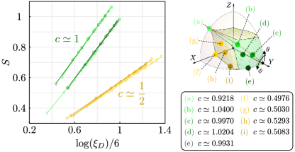
Figure 4: Finite-entanglement scaling $S\sim(c/6)\log\xi_{D}$ for the model Eq. (14). Here, $\xi_{D}$ is a correlation length computed via CTMRG with bond dimension $10\leq D\leq 80$. The plotted critical points correspond to the rotation axes $\vec{n}$ with (a) $\phi=\pi/4,\theta=\pi/2$, (b) $\phi=\theta=\pi/4$, (c) $\phi=\pi/4,\theta=\pi/8$, (d) $\phi=5\pi/16,\theta=3\pi/16$, (e) $\phi=\pi/2,\theta=\pi/8$, (f) $\phi=\theta=\pi/2$, (g) $\phi=5\pi/16,\theta=3\pi/8$, (h) $\phi=3\pi/8,\theta=5\pi/16$, and (i) $\phi=\pi/2,\theta=\pi/4$.

III.2.1 Random Rotation Noise within $XZ$-Plane

When $\vec{n}=(\sin\phi,0,\cos\phi)$ lies in the $XZ$-plane, the model Eq. (14) reduces to $\omega_{e}\propto 1+J(s_{v}s_{v^{\prime}}+\tau_{v}\tau_{v^{\prime}})+Ks_{v}s_{v^{\prime}}\tau_{v}\tau_{v^{\prime}}$ with

$$J=\frac{R\cos^{2}\phi}{2-R\cos^{2}\phi},\qquad K=\frac{2-R-R\sin^{2}\phi}{2-R\cos^{2}\phi},$$ (18)

which can be written as the Boltzmann weight $\omega_{e}\propto e^{\mathcal{J}(s_{v}s_{v^{\prime}}+\tau_{v}\tau_{v^{\prime}})+\mathcal{K}s_{v}s_{v^{\prime}}\tau_{v}\tau_{v^{\prime}}}$ of the isotropic AT model with coupling constants $\mathcal{J},\mathcal{K}\geq 0$. It is known that this model has three distinct phases (PO, FM, PM) [69], which is in accord with the $XZ$-plane of Fig. 1(b) and Fig. 3. For the pure $X$- and $Z$-rotations, the model simplifies further to a 2D Ising model on a square lattice, with a phase transition at $J_{c}=\frac{1}{2}\ln(1+\sqrt{2})$ [70, 71]. Thus, the phase boundary for the $X$- and $Z$-rotations is $R_{c}=2-\sqrt{2}\simeq 0.586$, which belongs to 2D Ising universality and extends into two Ising critical lines for $\phi\neq\pi/4$ [69].

The special cases with $(\phi,\theta)=(\pi/4,\pi/2)$ satisfy the self-duality condition $e^{-2\mathcal{K}}=\sinh(2\mathcal{J})$ [69]. In this scenario, the model remains in the PO phase for $R<1$ and reaches the Berezinskii-Kosterlitz-Thouless (BKT) transition point at $R=1$ [green dot in Fig. 1(b)]. This BKT transition was first discussed in Ref. [30] for the stochastic channel $\mathcal{E}_{e}[\rho]=(1-p)\rho+p(\vec{n}\cdot\vec{\sigma})_{e}\rho(\vec{n}\cdot\vec{\sigma})_{e}$ (for which $R=1$ corresponds to $p=1/2$), and our result greatly extends such transition for general distributions $g(\varphi_{e})$. It is shown in Ref. [30] that any transition in $|\rho_{D}\rangle\!\rangle$ is beyond the conventional anyon condensation scheme if $\mathcal{E}$ satisfies (i) electromagnetic duality (EMD) symmetry: $\mathbb{U}_{D}\mathbb{E}\mathbb{U}_{D}^{\dagger}=\mathbb{E}$ for $\mathbb{U}_{D}=\prod_{e}\frac{1}{2}(X_{e}+Z_{e})(\bar{X}_{e}+\bar{Z}_{e})$, and (ii) partial transpose symmetry: $(\mathbb{E}^{\dagger}\mathbb{E})^{T_{\mathcal{H}}}=(\mathbb{E}^{\dagger}\mathbb{E})^{\bar{T}_{\bar{\mathcal{H}}}}=\mathbb{E}^{\dagger}\mathbb{E}$. One can easily check that $\mathbb{E}_{\mathrm{rot}}$ [see Eq. (13)] with $(\phi,\theta)=(\pi/4,\pi/2)$ satisfies both the EMD and partial transpose symmetries. Therefore, this BKT transition is an unconventional topological phase transition for any $g(\varphi_{e})$ achieving $R=1$. Such a case involves a non-stochastic noise $\mathcal{E}_{\mathrm{rot}}$ with respect to asymmetric distributions with vanishing second Fourier coefficient, e.g., $g(\varphi_{e})=(2\pi)^{-1}(1+\sin\varphi_{e}\cos 2\varphi_{e})$.

III.2.2 Random $Y$-Rotation Noise

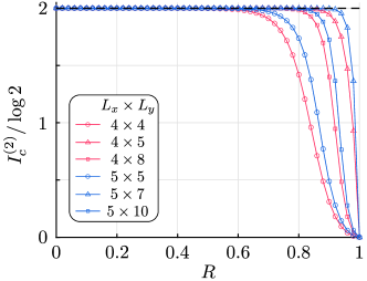
Figure 5: Rényi-2 coherent information $I_{c}^{(2)}$ of decohered toric code under random $Y$-rotation noise on various $L_{x}\times L_{y}$ torus geometry.

The green phase boundaries with $R=1$ in Fig. 1(b) demonstrate that the mixed-state topological order is remarkably stable against random rotation noise with $\vec{n}$ near the $Y$-axis ($\theta=\phi=0$), suggesting that the QEC is possible in principle for the TC under such noise. This stability can be understood analytically for the pure $Y$-rotation, for which the model Eqs. (14) becomes

$$\omega_{e}\propto 1+\frac{R}{2-R}(s_{v}s_{v^{\prime}}-\tau_{v}\tau_{v^{\prime}})+s_{v}s_{v^{\prime}}\tau_{v}\tau_{v^{\prime}}.$$ (19)

In Appendix B.4, we map Eq. (19) to a certain vertex model called the “staggered vertex” model. We analytically compute the transfer matrix and examine the correlation length, order parameter, and anyon parameters (see Appendix. B.4 for details). We find that the model has no phase transition for $R<1$ and undergoes spontaneous symmetry breaking at $R=1$. This suggests that double $\mathbb{Z}_{2}$ topological order persists for $R<1$, which is consistent with previous numerical results.

For coherent information, we numerically compute $I_{c}^{(2)}$ from Eq. (17) for finite-sized systems. Figure 5 shows the result for various $L_{x}\times L_{y}$ torus geometries. Even in small systems, $I_{c}^{(2)}$ converges quite well to $2\log 2$ for $R<1$. At $R=1$, we have $I_{c}^{(2)}=0$ and the quantum memory is lost. An intriguing point to note is that $I_{c}^{(2)}$ goes to 1 rapidly for geometries with $\gcd(L_{x},L_{y})=1$. This aligns with the fact that the TC with coprime geometry has an advantage in correcting stochastic Pauli-$Y$ noise [72].

Although $I_{c}^{(2)}$ does not rigorously guarantee the existence of the QEC protocol, we expect the same behavior to persist in the replica limit $n\rightarrow 1$. This anticipation is consistent with previous studies that demonstrated the error threshold of the TC against stochastic $Y$ noise to be $p_{c}=0.5$ [73, 72, 74]. Additionally, the decohered TC under the maximal stochastic $Y$ noise has a diverging Markov length [41], which has been proposed to play a role similar to the correlation length in pure states [22]. This fact suggests that there should be a mixed-state phase transition at $R_{c}=1$. We also note the similar robustness of the TC in the measurement setup, where a $Y$-measurement probability of unity is required to destroy the encoded quantum memory in the thermodynamic limit [75, 76].

III.2.3 Critical Region with $c=1/2$

The Ising critical lines identified within the $XZ$ plane in Sec. III.2.1 are part of the yellow phase boundaries in Fig. 1(b), which separate regions of double and single $\mathbb{Z}_{2}$ topological orders. Notably, these entire two-dimensional phase boundaries exhibit Ising criticality ($c=1/2$). We believe that this arises from the non-Hermiticity of the effective stat-mech model Eq. (14), which at the field-theory level may introduce an imaginary mass term that is reported to extend the Ising criticality [77]. This instance illustrates the importance of studying non-Hermitian stat-mech models to understand quantum many-body states under decoherence, a direction that deserves further investigation.

III.2.4 Critical Region with $c=1$

Spreading out from the BKT transition point at $\vec{n}_{\text{BKT}}=(1/\sqrt{2},0,1/\sqrt{2})$ [green dot in Fig. 1(b)], the green phase boundaries with $R=1$ form an extended critical region with a central charge $c=1$, except for the pure $Y$-rotation case $\vec{n}_{Y}=(0,1,0)$. We expect that this extended critical region may be described by a non-unitary conformally field theory with an effective central charge $c_{*}=1$. It will be interesting to further investigate the precise nature of this critical region for future work.

We expect that the mixed-state transitions at the green phase boundary cannot be described by the standard anyon condensation scheme, as in the BKT transition point $\vec{n}_{\text{BKT}}$. A notable point is that Eq. (13) with a general rotation axis $\vec{n}$ pointing within the green critical region does not satisfy the EMD and/or partial-transpose symmetries discussed in Sec. III.2.1. This suggests that this critical region may provide an example of an unconventional mixed-state phase transition beyond the sufficient conditions for such a transition derived in Ref. [30], which deserves future investigation.

III.2.5 Phase Diagram in the Replica Limit

Finally, we discuss the potential structure of the phase diagram of $\rho_{D}$ in the replica limit $n\rightarrow 1$. While the doubled Hilbert space formalism offers insights into phase structures, the actual phase boundaries and universality for $n=1$ may differ. For example, the TC under incoherent $X$/$Z$ noise follows the 2D random-bond Ising model (RBIM) universality [4, 17, 18, 19] rather than the 2D Ising universality obtained from the doubled Hilbert space formalism. Based on this, we conjecture that the yellow phase boundaries fall within the 2D RBIM universality class for $n=1$. Another interesting question is whether the green phase boundary remains critical at $n=1$ and how its shape changes. Since the phase boundary for pure $Y$-rotation appears to stay at $R_{c}=1$ in the replica limit (see Sec. III.2.2), one might consider three potential scenarios: (i) two isolated points at $\vec{n}_{\text{BKT}}$ and $\vec{n}_{Y}$ with $R=1$, (ii) a critical curve $\phi=\pi/4$ connecting these two points, and (iii) a critical region with these points as its vertices. In each case, we believe that the pure $Y$-rotation point $\vec{n}_{Y}$ is not critical.

III.3 Example: Double von Mises Distribution

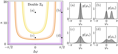
Figure 6: Phase diagram of toric code under random rotation noise with respect to the double von-Mises distribution $g_{\kappa,\Delta\varphi}(\varphi_{e})$ [see Eq. (21)]. The yellow/orange/purple curves correspond to phase boundaries for $\vec{n}=(1,0,0)$ / $(1/\sqrt{2},1/\sqrt{2},0)$ / $(0,1,0)$, respectively. The double (single) $\mathbb{Z}_{2}$ topological order is within the region (not) surrounded by the shade for each $\vec{n}$. The distribution profiles on the right show $g_{\kappa,\Delta\varphi}(\varphi_{e})$ with (a) $\kappa=15,\Delta\varphi=0$, (b) $\kappa=15,\Delta\varphi=\pi/2$, (c) $\kappa=3,\Delta\phi=0$, and (d) $\kappa=3,\Delta\varphi=\pi/2$.

In this section, we provide an exemplary mixed-state phase diagram for parameters characterizing a certain angle distribution. A von Mises (vM) distribution is defined as

$$h_{\kappa,\varphi}(\varphi_{e})=\frac{e^{\kappa\cos(\varphi_{e}-\varphi)}}{2\pi I_{0}(\kappa)},$$ (20)

where $I_{\alpha}(\kappa)$ is the modified Bessel function of the first kind of order $\alpha$. The distribution Eq. (20) has a mean $\varphi$ and a variance $1-I_{1}(\kappa)/I_{0}(\kappa)$. Since $1-I_{1}(\kappa)/I_{0}(\kappa)\rightarrow(2\kappa)^{-1}$ as $\kappa\rightarrow\infty$, we can interpret $\kappa^{-1}$ as a measure of concentration. As $\kappa\rightarrow 0$ ($\infty$), Eq. (20) approaches the uniform (Dirac delta) distribution on $[-\pi,\pi)$. We consider a double vM distribution $g(\varphi_{e})$, a convex combination of two vM distributions, as a concrete example of an angle distribution:

$$g_{\kappa,\Delta\varphi}(\varphi_{e})=qh_{\kappa,0}(\varphi_{e})+(1-q)h_{\kappa,\Delta\varphi}(\varphi_{e}),$$ (21)

where $q\in[0,1]$ controls the mixedness between the two vM distributions, $\kappa$ controls the width of each peak, and $\Delta\varphi$ is the distance between the two peaks. For $q=1/2$, we have $R=[I_{2}(\kappa)/I_{0}(\kappa)]^{2}\cos^{2}(\Delta\varphi)$. Solving $R=R_{c}$, with $R_{c}$ being a critical point lying at the intersection of $\vec{n}$ and the phase boundaries in Fig. 1(b), one can obtain a phase diagram with respect to $\kappa$ and $\Delta\varphi$. Fig. 6 shows the resulting phase diagram for the distribution Eq. (21) with $q=1/2$. Fig. 6 illustrates that clear distinguishability between the two peaks (maximal at $\Delta\varphi=\pm\pi/2$) tends to degrade the quantum memory. It also breaks down for flat peaks (more precisely, $\kappa<5.015$). The nontrivial point is that when $\vec{n}$ has sufficiently large $n_{y}$ so that it points within the green phase boundary, the quantum memory is robust regardless of the distinguishability between peaks and their width.

IV Amplitude Damping Noise

In this section, we study decohered TC under amplitude damping noise. The amplitude damping channel models the decay process of an excited state of a qubit via the spontaneous emission of a photon. Specifically, the channel is defined as $\mathcal{E}_{\mathrm{amp}}\equiv\prod_{e}\mathcal{E}_{e}$, where $\mathcal{E}_{e}[\rho]\equiv K_{0,e}\rho K_{0,e}^{\dagger}+K_{1,e}\rho K_{1,e}^{\dagger}$ and the Kraus operators are given by

$$K_{0,e}=\begin{pmatrix}1&0\\ 0&\sqrt{1-\gamma}\end{pmatrix},\qquad K_{1,e}=\begin{pmatrix}0&\sqrt{\gamma}\\ 0&0\end{pmatrix}.$$ (22)

The damping parameter $\gamma\in[0,1]$ depends on the rate of spontaneous emission [see Fig. 1(a)]. The amplitude damping channel is a typical coherent noise in NISQ devices [51] and cannot be expressed as a stochastic Pauli channel. We are interested in $\rho_{D}=\mathcal{E}_{\mathrm{amp}}[\rho_{0}]$.

As in Sec. III.1, we can compute the purity $\mathrm{Tr}[\rho_{D}^{2}]=\langle\!\langle\rho_{0}|\mathbb{E}_{\mathrm{amp}}^{\dagger}\mathbb{E}_{\mathrm{amp}}|\rho_{0}\rangle\!\rangle$, where $\mathbb{E}_{\mathrm{amp}}=\prod_{e}\mathbb{E}_{e}$ is given by $\mathbb{E}_{e}=K_{0,e}\otimes\bar{K}_{0,e}+K_{1,e}\otimes\bar{K}_{1,e}$. In Appendix C, we show that the purity can be written as $\mathrm{Tr}[\rho_{D}]\propto\sum_{\mathbf{s}_{v},\bm{\tau}_{v}}\prod_{e}\omega_{e}$, where $s_{v}$ and $\tau_{v}$ are Ising spins on the vertices and the local weight is given by $\omega_{e}\propto 1+J_{+}s_{v}s_{v^{\prime}}-J_{-}\tau_{v}\tau_{v^{\prime}}+Ks_{v}s_{v^{\prime}}\tau_{v}\tau_{v^{\prime}}$ with

$$J_{\pm}=\frac{\gamma(1\pm\gamma)}{\gamma^{2}-\gamma+2},\qquad K=\frac{\gamma^{2}-3\gamma+2}{\gamma^{2}-\gamma+2}.$$ (23)

For $\gamma\in[0,1]$, $\omega_{e}$ with Eq. (23) corresponds to the local Boltzmann weight of the anisotropic AT model (see Appendix C for details). The phase diagram must be symmetric about $\gamma=1/2$ since the stat-mech model is symmetric with respect to $\gamma\leftrightarrow 1-\gamma$. (This transformation exchanges $J_{+}$ and $K$, which does not affect the partition function $\sum_{\mathbf{s}_{v},\bm{\tau}_{v}}\prod_{e}\omega_{e}$ due to its invariance under the permutation of $s$ and $st$ spins.)

In the absence of decoherence ($\gamma=0$), the weight reduces to $\omega_{e}\propto 1+s_{v}s_{v^{\prime}}\tau_{v}\tau_{v^{\prime}}$, indicating that the model is in the PO phase with $\langle s_{v}\tau_{v}\rangle=1$ and $\langle s_{v}\rangle=\langle\tau_{v}\rangle=0$. On the other hand, when all spins are polarized to the ground state ($\gamma=1$), the weight reduces to $\omega_{e}\propto 1+s_{v}s_{v^{\prime}}$ and hence the model has $\langle s_{v}\rangle=1$ and $\langle\tau_{v}\rangle=\langle s_{v}\tau_{v}\rangle=0$. Thus, one might expect only two phases: the PO phase at small $\gamma$, and the phase with ordered $s$ spins at large $\gamma$. In addition to these two phases, we find from the CTMRG simulation an intermediate PM phase with $\langle\tau_{v}\rangle=\langle s_{v}\rangle=\langle s_{v}\tau_{v}\rangle=0$ in a narrow parameter regime $0.487<\gamma<0.513$ (see Fig. 7). Therefore, the amplitude damping channel makes the decohered TC undergo two successive topological phase transitions, even though it has only one tuning parameter $\gamma$. This phenomenon has also been observed numerically in Ref. [37] using different schemes, and our work provides a solid stat-mech model underlying it.

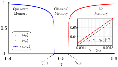
Figure 7: Order parameters $\langle s_{v}\rangle$, $\langle\tau_{v}\rangle$, and $\langle s_{v}\tau_{v}\rangle$ of the statistical mechanics model Eq. (23) associated with the decohered toric code under amplitude damping noise. The model undergoes two phase transitions at $\gamma_{c,1}\simeq 0.487$ and $\gamma_{c,2}\simeq 0.513$, beyond each of which the quantum memory degrades to classical memory and no memory properties remain. The inset (log-log scale) shows the scaling of $\langle s_{v}\rangle$ above $\gamma_{c,2}$ with the Ising critical exponent $\beta=1/8$.

The anyon parameters are identical to Eqs. (16), from which we can learn which anyons condense: The first phase transition at $\gamma_{c,1}\simeq 0.487$ condenses $m\bar{m}$ anyons and degrades the quantum memory to classical memory. Subsequently, the second phase transition at $\gamma_{c,2}\simeq 0.513$ condenses $e\bar{e}$ anyons, trivializing the classical memory. This coincides with almost all spins polarizing to the ground state for large $\gamma$. The overall phase diagram is shown in Fig. 1(c). The numerics show that the two transitions belong to the 2D Ising universality with critical exponent $\beta=1/8$ (see inset of Fig. 7). The Rényi-2 coherent information is also given by Eq. (17), and an argument similar to the one in Sec. III.2 can be used to show that $I_{c}^{(2)}$ in the thermodynamic limit is equal to $2\log 2$, $0$, and $-2\log 2$ for the PO, PM, and the $s$-ordered phases, respectively. This is consistent with the analysis from the anyon parameters.

V Discussion

In this work, we explore the mixed-state phase of the decohered toric code under two representative coherent noises using the doubled Hilbert space formalism. For random rotation noise, we determine the phase diagram for any rotation axis and arbitrary angle distribution, significantly generalizing the previously studied incoherent noise models. In addition to the robust quantum memory observed under random rotations about axes near the $Y$-axis, we identify phase boundaries featuring several interesting properties, such as Ising critical surfaces and unconventional mixed-state phase transitions, which merit further investigation. For the amplitude damping noise, we uncover two mixed-state topological phase transitions governed by a single parameter $\gamma$.

We remark that the phase boundaries for the random rotation error identified here differ from the error threshold under global unitary rotation obtained in Ref. [50], where the decoding problem maps to a Majorana network. This difference stems from practical constraints in standard QEC schemes, where syndromes are obtained by measuring check operators (e.g., $A_{v}$ and $B_{p}$) and Pauli recovery operations are applied. In contrast, our mixed-state setup addresses the intrinsic noise threshold of the decohered toric code, within which QEC is possible in principle, though the corresponding QEC protocol may require experimentally challenging operations. It would be interesting to determine the “practical” error threshold for coherent noises, such as amplitude damping noise, as done for global rotation error [50]. The stat-mech mapping technique and tensor network method employed in this work seem straightforwardly applicable in this direction.

As mentioned in Sec. III.2.4, it will be worthwhile to understand the precise conditions for an unconventional mixed-state phase transition. Moreover, an important open question is whether the structure of our mixed-state phase diagrams under coherent noises persists in the replica limit $n\rightarrow 1$. For coherent noises, exact diagonalization of the decohered density matrix, as done for incoherent noises [18, 19], is challenging. Developing new analytical and numerical frameworks to access the replica limit directly would be valuable for further study. It would also be intriguing to explore whether coherent noises can induce novel mixed-state phases beyond those captured by the doubled Hilbert space formalism.

Note added: While completing this work, we became aware of related independent work that studies the error threshold of the surface code under generic unitary rotation errors using the mapping to a disordered non-Hermitian AT model [78].

Appendix A General Mapping for Anyon Parameters and Coherent Information

In this appendix, we review the mapping of anyon condensation/confinement parameters to an observable in the stat-mech model [Eqs. (9)], which was introduced in Ref. [30], for the sake of self-containedness. We then derive the stat-mech expression for the Rényi-2 coherent information [Eqs. (34) and (36)].

A.1 Anyon Condensation/Confinement Parameters

Consider a state $\rho_{0}^{e\bar{e}}=w_{e}(l)\rho_{0}w_{e}^{\dagger}(l)$, where $w_{e}(l)=\prod_{e\in l}Z_{e}$ is a string operator creating a pair of $e$ anyons at the endpoints $i$ and $j$ of an open string $l$ on the original lattice. From Eq. (4), the associated Choi state $|\rho_{0}^{e\bar{e}}\rangle\!\rangle=w_{e}(l)\bar{w}_{e}(l)|\rho_{0}\rangle\!\rangle$ is given by

$$|\rho_{0}^{e\bar{e}}\rangle\!\rangle$$ (24)

$$\propto\sum_{\begin{subarray}{c}\mathbf{z}_{e},\bar{\mathbf{z}}_{e},\\ \mathbf{x}_{v},\bar{\mathbf{x}}_{v}\end{subarray}}\prod_{e\in l}z_{e}\bar{z}_{e}\prod_{e}(1+z_{e}x_{v}x_{v^{\prime}})(1+\bar{z}_{e}\bar{x}_{v}\bar{x}_{v^{\prime}})|\mathbf{z}_{e},\bar{\mathbf{z}}_{e}\rangle\!\rangle$$

$$=\sum_{\begin{subarray}{c}\mathbf{z}_{e},\bar{\mathbf{z}}_{e},\\ \mathbf{x}_{v},\bar{\mathbf{x}}_{v}\end{subarray}}x_{i}\bar{x}_{i}x_{j}\bar{x}_{j}\prod_{e}(1+z_{e}x_{v}x_{v^{\prime}})(1+\bar{z}_{e}\bar{x}_{v}\bar{x}_{v^{\prime}})|\mathbf{z}_{e},\bar{\mathbf{z}}_{e}\rangle\!\rangle,$$

where we have used $z_{e}\bar{z}_{e}(1+z_{e}x_{v}x_{v^{\prime}})(1+\bar{z}_{e}\bar{x}_{v}\bar{x}_{v^{\prime}})=x_{v}x_{v^{\prime}}\bar{x}_{v}\bar{x}_{v^{\prime}}(1+z_{e}x_{v}x_{v^{\prime}})(1+\bar{z}_{e}\bar{x}_{v}\bar{x}_{v^{\prime}})$ in the second line. Since the action of $\mathbb{E}$ does not affect the additional $x_{i}\bar{x}_{i}x_{j}\bar{x}_{j}$ factor, we obtain

$$\langle\!\langle I\bar{I}|e\bar{e}\rangle\!\rangle =\lim_{|i-j|\rightarrow\infty}\frac{\sum_{\mathbf{x}_{v},\bar{\mathbf{x}}_{v},\mathbf{t}_{v},\bar{\mathbf{t}}_{v}}x_{i}\bar{x}_{i}x_{j}\bar{x}_{j}\prod_{e}\omega_{e}}{\sum_{\mathbf{x}_{v},\bar{\mathbf{x}}_{v},\mathbf{t}_{v},\bar{\mathbf{t}}_{v}}\prod_{e}\omega_{e}}$$ (25)

$$=\lim_{|i-j|\rightarrow\infty}\langle x_{i}\bar{x}_{i}x_{j}\bar{x}_{j}\rangle,$$

where $\omega_{e}$ is given by Eq. (6). Notice that the effect of applying $w_{e}(l)$ ($\bar{w}_{e}(l)$) on $|\rho_{0}\rangle\!\rangle$ is to add a factor $x_{i}x_{j}$ ($\bar{x}_{i}\bar{x}_{j}$). Using this, one can similarly show $\langle\!\langle e\bar{I}|e\bar{I}\rangle\!\rangle=\lim_{|i-j|\rightarrow\infty}\langle x_{i}t_{i}x_{j}t_{j}\rangle$.

Next, consider $\rho_{0}^{m\bar{m}}=w_{m}(\tilde{l})\rho_{0}w_{m}^{\dagger}(\tilde{l})$, where $w_{m}(\tilde{l})=\prod_{m\in\tilde{l}}X_{e}$ is a string operator creating a pair of $m$ anyons at the endpoints $\tilde{i}$ and $\tilde{j}$ of an open string $\tilde{l}$ on the dual lattice. Since the $X_{e}$ operator flips $z_{e}$ to $-z_{e}$ in Eq. (4) (and similarly for $\bar{X}_{e}$), the Choi state $|\rho_{0}^{m\bar{m}}\rangle\!\rangle=w_{m}(l)\bar{w}_{m}(l)|\rho_{0}\rangle\!\rangle$ is given by

$$|\rho_{0}^{m\bar{m}}\rangle\!\rangle \propto\sum_{\begin{subarray}{c}\mathbf{z}_{e},\bar{\mathbf{z}}_{e},\\ \mathbf{x}_{v},\bar{\mathbf{x}}_{v}\end{subarray}}\prod_{e}(1+\eta_{e}z_{e}x_{v}x_{v^{\prime}})(1+\eta_{e}\bar{z}_{e}\bar{x}_{v}\bar{x}_{v^{\prime}})|\mathbf{z}_{e},\bar{\mathbf{z}}_{e}\rangle\!\rangle,$$ (26)

where $\eta_{e}=-1$ if $e\in\tilde{l}$, and $1$ otherwise. It follows that

$$\langle\!\langle I\bar{I}|m\bar{m}\rangle\!\rangle=\lim_{|\tilde{i}-\tilde{j}|\rightarrow\infty}\frac{\sum_{\mathbf{x}_{v},\bar{\mathbf{x}}_{v},\mathbf{t}_{v},\bar{\mathbf{t}}_{v}}\prod_{e}\omega_{e}^{\eta}}{\sum_{\mathbf{x}_{v},\bar{\mathbf{x}}_{v},\mathbf{t}_{v},\bar{\mathbf{t}}_{v}}\prod_{e}\omega_{e}},$$ (27)

where

$$\omega_{e}^{\eta}\equiv\sum_{z_{e},\bar{z}_{e},z^{\prime}_{e},\bar{z}^{\prime}_{e}=\pm 1}\langle\!\langle z^{\prime}_{e},\bar{z}^{\prime}_{e}|\mathbb{E}_{e}^{\dagger}\mathbb{E}_{e}|\eta_{e}z_{e},\eta_{e}\bar{z}_{e}\rangle\!\rangle$$ (28)

$$\hskip 5.0pt\times(1+z_{e}x_{v}x_{v^{\prime}})(1+\bar{z}_{e}\bar{x}_{v}\bar{x}_{v^{\prime}})(1+z^{\prime}_{e}t_{v}t_{v^{\prime}})(1+\bar{z}^{\prime}_{e}\bar{t}_{v}\bar{t}_{v^{\prime}}).$$

Note that the sign of interactions $x_{v}x_{v^{\prime}}$ and $\bar{x}_{v}\bar{x}_{v^{\prime}}$ are flipped along $\tilde{l}$ in Eq. (28) compared to Eq. (6). Therefore, we obtain $\langle\!\langle I\bar{I}|m\bar{m}\rangle\!\rangle=\lim_{|\tilde{i}-\tilde{j}|\rightarrow\infty}\langle\mu_{\tilde{i}}^{x}\mu_{\tilde{i}}^{\bar{x}}\mu_{\tilde{j}}^{x}\mu_{\tilde{j}}^{\bar{x}}\rangle$, where $\mu^{x}$ and $\mu^{\bar{x}}$ are the disorder parameters of $x$ and $\bar{x}$ spins, respectively [64]. Observing that the effect of $w_{m}(\tilde{l})$ ($\bar{w}_{m}(\tilde{l})$) on $|\rho_{0}\rangle\!\rangle$ is to flip the sign of interactions $x_{v}x_{v^{\prime}}$ ($\bar{x}_{v}\bar{x}_{v^{\prime}}$) along $\tilde{l}$, one can similarly derive $\langle\!\langle m\bar{I}|m\bar{I}\rangle\!\rangle=\lim_{|\tilde{i}-\tilde{j}|\rightarrow\infty}\langle\mu_{\tilde{i}}^{x}\mu_{\tilde{i}}^{t}\mu_{\tilde{j}}^{x}\mu_{\tilde{j}}^{t}\rangle$. This completes the proof of the correspondence Eq. (9).

A.2 Coherent Information

The logical operators of the TC are given by $\mathbf{Z}_{1,2}\equiv\prod_{e\in l_{1,2}}Z_{e}$ and $\mathbf{X}_{1,2}\equiv\prod_{e\in\tilde{l}_{1,2}}X_{e}$, where $l_{1,2}$ ($\tilde{l}_{1,2}$) are two non-contractible loops on the original (dual) lattice. Let $|\Psi_{0}\rangle$ be the ground state satisfying $\mathbf{Z}_{1,2}|\Psi_{0}\rangle=|\Psi_{0}\rangle$. Then, the four ground states can be written as $|\Psi_{0}^{a,b}\rangle\equiv\mathbf{X}_{1}^{a}\mathbf{X}_{2}^{b}|\Psi_{0}\rangle$ with $a,b\in\{0,1\}$. These ground states can be obtained from Eq. (3) by applying $\mathbf{X}_{1,2}$ properly, which flips $z_{e}$ to $-z_{e}$ for $e\in\tilde{l}_{1,2}$ in Eq. (3).

Now, we express the Rényi-2 coherent information $I_{c}^{(2)}$ in terms of the stat-mech model Eq. (5). Let $Q$ be the TC system and $R$ be the two-qubit reference system, forming two Bell pairs with two logical qubits of $Q$. The density matrices for $RQ$ and $Q$ before channel $\mathcal{E}$ are given by

$$\rho_{0,RQ} =\frac{1}{4}\sum_{\begin{subarray}{c}a,b=0,1\\ a^{\prime},b^{\prime}=0,1\end{subarray}}|a,b\rangle\langle a^{\prime},b^{\prime}|_{R}\otimes|\Psi_{0}^{a,b}\rangle\langle\Psi_{0}^{a^{\prime},b^{\prime}}|_{Q},$$ (29)

$$\rho_{0,Q} =\frac{1}{4}\sum_{a,b=0,1}|\Psi_{0}^{a,b}\rangle\langle\Psi_{0}^{a,b}|_{Q},$$

where $|a,b\rangle_{R}$ are orthonormal states in $R$. Let $\eta_{e}=-1$ ($\zeta_{e}=-1$) if $e\in l_{1}$ ($e\in l_{2}$) and $1$ otherwise. Using $\mathrm{Tr}[\rho^{2}]=\langle\!\langle\rho|\rho\rangle\!\rangle$ and Eq. (4), one can obtain

$$\mathrm{Tr}[\mathcal{E}[\rho_{0,RQ}]^{2}] \propto\sum_{\begin{subarray}{c}a,b=0,1\\ a^{\prime},b^{\prime}=0,1\end{subarray}}\underbrace{\sum_{\mathbf{x}_{v},\bar{\mathbf{x}}_{v},\mathbf{t}_{v},\bar{\mathbf{t}}_{v}}\prod_{e}\omega_{e}^{aba^{\prime}b^{\prime}}}_{\equiv\,\mathcal{Z}^{aba^{\prime}b^{\prime}}},$$ (30)

$$\mathrm{Tr}[\mathcal{E}[\rho_{0,Q}]^{2}] \propto\sum_{\begin{subarray}{c}a,b=0,1\\ a^{\prime},b^{\prime}=0,1\end{subarray}}\underbrace{\sum_{\mathbf{x}_{v},\bar{\mathbf{x}}_{v},\mathbf{t}_{v},\bar{\mathbf{t}}_{v}}\prod_{e}\widetilde{\omega}_{e}^{aba^{\prime}b^{\prime}}}_{\equiv\,\widetilde{\mathcal{Z}}^{aba^{\prime}b^{\prime}}},$$ (31)

where

$$\omega_{e}^{aba^{\prime}b^{\prime}}\equiv\!\!\sum_{\begin{subarray}{c}z_{e},\bar{z}_{e},\\ z^{\prime}_{e},\bar{z}^{\prime}_{e}=\pm 1\end{subarray}}\!\!\langle\!\langle\eta_{e}^{a}\zeta_{e}^{b}z^{\prime}_{e},\eta_{e}^{a^{\prime}}\zeta_{e}^{b^{\prime}}\bar{z}^{\prime}_{e}|\mathbb{E}_{e}^{\dagger}\mathbb{E}_{e}|\eta_{e}^{a}\zeta_{e}^{b}z_{e},\eta_{e}^{a^{\prime}}\zeta_{e}^{b^{\prime}}\bar{z}_{e}\rangle\!\rangle$$

$$\hskip 5.0pt\times(1+z_{e}x_{v}x_{v^{\prime}})(1+\bar{z}_{e}\bar{x}_{v}\bar{x}_{v^{\prime}})(1+z^{\prime}_{e}t_{v}t_{v^{\prime}})(1+\bar{z}^{\prime}_{e}\bar{t}_{v}\bar{t}_{v^{\prime}}),$$ (32)

$$\widetilde{\omega}_{e}^{aba^{\prime}b^{\prime}}\equiv\!\!\sum_{\begin{subarray}{c}z_{e},\bar{z}_{e},\\ z^{\prime}_{e},\bar{z}^{\prime}_{e}=\pm 1\end{subarray}}\!\!\langle\!\langle\eta_{e}^{a}\zeta_{e}^{b}z^{\prime}_{e},\eta_{e}^{a}\zeta_{e}^{b}\bar{z}^{\prime}_{e}|\mathbb{E}_{e}^{\dagger}\mathbb{E}_{e}|\eta_{e}^{a^{\prime}}\zeta_{e}^{b^{\prime}}z_{e},\eta_{e}^{a^{\prime}}\zeta_{e}^{b^{\prime}}\bar{z}_{e}\rangle\!\rangle$$

$$\hskip 5.0pt\times(1+z_{e}x_{v}x_{v^{\prime}})(1+\bar{z}_{e}\bar{x}_{v}\bar{x}_{v^{\prime}})(1+z^{\prime}_{e}t_{v}t_{v^{\prime}})(1+\bar{z}^{\prime}_{e}\bar{t}_{v}\bar{t}_{v^{\prime}}),$$ (33)

The weights Eqs. (32) and (33) are nothing but the original weight Eq. (6) with the sign of interactions flipped along non-contractible loops according to the labels $(a,b,a^{\prime},b^{\prime})$. Note that $\omega_{e}^{0000}=\widetilde{\omega}_{e}^{0000}=\omega_{e}$. Finally, the Rényi-2 coherent information becomes [see Eq. (10)]

$$I_{c}^{(2)}(R\rangle Q)=\log\left(\frac{\sum_{a,b,a^{\prime},b^{\prime}=0,1}e^{-\Delta F^{aba^{\prime}b^{\prime}}}}{\sum_{a,b,a^{\prime},b^{\prime}=0,1}e^{-\Delta\widetilde{F}^{aba^{\prime}b^{\prime}}}}\right).$$ (34)

where $\Delta F^{aba^{\prime}b^{\prime}}\equiv-\log(\mathcal{Z}^{aba^{\prime}b^{\prime}}/\mathcal{Z}^{0000})$ is the free energy cost of forming defects along the non-contractible loops corresponding to $\omega_{e}^{aba^{\prime}b^{\prime}}$ (and similarly for $\Delta\widetilde{F}^{aba^{\prime}b^{\prime}}$).

This expression for $I_{c}^{(2)}$ can be simplified further for the coherent noises considered in this paper, where the weight $\omega_{e}$ is of the Ashkin-Teller type: $\omega_{e}\propto 1+J_{1}s_{v}s_{v^{\prime}}+J_{2}\tau_{v}\tau_{v^{\prime}}+Ks_{v}s_{v^{\prime}}\tau_{v}\tau_{v^{\prime}}$, with $s_{v}=x_{v}\bar{x_{v}}$ and $\tau_{v}=\bar{x}_{v}t_{v}$ [see Eqs. (14), (15), and (23)]. In such cases, Eqs. (32) and (33) reduce to

$$\omega_{e}^{ab} \propto 1+\eta_{e}^{a}\zeta_{e}^{b}(J_{1}s_{v}s_{v^{\prime}}+J_{2}\tau_{v}\tau_{v^{\prime}})+Ks_{v}s_{v^{\prime}}\tau_{v}\tau_{v^{\prime}},$$ (35)

$$\widetilde{\omega}_{e}^{ab} \propto 1+J_{1}s_{v}s_{v^{\prime}}+\eta_{e}^{a}\zeta_{e}^{b}(J_{2}\tau_{v}\tau_{v^{\prime}}+Ks_{v}s_{v^{\prime}}\tau_{v}\tau_{v^{\prime}}),$$

where we redefined labels as $a+a^{\prime}\rightarrow a$ and $b+b^{\prime}\rightarrow b$. Accordingly, Eq. (34) simplifies to Eq. (17):

$$I_{c}^{(2)}(R\rangle Q)=\log\left(\frac{\sum_{a,b=0,1}e^{-\Delta F_{s,\tau}^{ab}}}{\sum_{a,b=0,1}e^{-\Delta F_{\tau,s\tau}^{ab}}}\right),$$ (36)

where $\Delta F_{s,\tau}^{ab}$ is the free energy cost of forming defects in the interactions $s_{v}s_{v^{\prime}}$ and $\tau_{v}\tau_{v^{\prime}}$ along the non-contractible loop pattern $(a,b)$ (and similarly for $\Delta F_{s,s\tau}^{ab}$).

Appendix B Details on Random Rotation Noises

In this appendix, we elaborate on the random rotation noise discussed in Sec. III. We prove the reduction of Eq. (11) to stochastic $\vec{n}\cdot\vec{\sigma}$ noise and the $R$-dependence of the effective stat-mech model. We also detail the mapping to the stat-mech model Eq. (14) and solve the staggered vertex model for the $Y$-rotation noise discussed in Sec. III.2.2.

B.1 Reduction to Stochastic Noise

Here, we show that random rotation channel Eq. (11) reduces to a stochastic $\vec{n}\cdot\vec{\sigma}$ noise when the distribution $g(\varphi_{e})$ is even. We expand the global unitary rotation as

$$\prod_{e}U_{e}(\varphi_{e})=\sum_{\mathcal{C}}A_{-}(\mathcal{C},\boldsymbol{\varphi})O_{\mathcal{C}}^{(\vec{n})}$$ (37)

where $\mathcal{C}$ runs over all subsets, $O_{\mathcal{C}}^{(\vec{n})}\equiv\prod_{e\in\mathcal{C}}(\vec{n}\cdot\vec{\sigma})_{e}$, and

$$A_{\pm}(\mathcal{C},\boldsymbol{\varphi})\equiv\prod_{e\not\in\mathcal{C}}\cos\varphi_{e}\prod_{e\in\mathcal{C}}(\pm i\sin\varphi_{e}).$$ (38)

The decohered state $\rho_{D}=\mathcal{E}[\rho_{0}]$ can then be written as $\rho_{D}=\sum_{\mathcal{C},\bar{\mathcal{C}}}\mathcal{A}(\mathcal{C},\bar{\mathcal{C}})O_{\mathcal{C}}^{(\vec{n})}\rho_{0}O_{\bar{\mathcal{C}}}^{(\vec{n})}$ with $\mathcal{A}(\mathcal{C},\bar{\mathcal{C}})\equiv\int\prod_{e}d\varphi_{e}g(\varphi_{e})A_{-}(\mathcal{C},\boldsymbol{\varphi})A_{+}(\mathcal{C},\boldsymbol{\varphi})$. When $g(\varphi_{e})$ is even, the coefficient $\mathcal{A}(\mathcal{C},\bar{\mathcal{C}})$ simplifies as follows:

$$\mathcal{A}(\mathcal{C},\bar{\mathcal{C}}) =\int\prod_{e}d\varphi_{e}g(\varphi_{e})\prod_{e\not\in\mathcal{C},\bar{\mathcal{C}}}\cos^{2}\varphi_{e}\prod_{e\in\mathcal{C},\bar{\mathcal{C}}}\sin^{2}\varphi_{e}$$ (39)

$$\hskip 7.0pt\times\prod_{e\in\mathcal{C},e\not\in\bar{\mathcal{C}}}\!(-i\cos\varphi_{e}\sin\varphi_{e})\!\prod_{e\not\in\mathcal{C},e\in\bar{\mathcal{C}}}\!(i\cos\varphi_{e}\sin\varphi_{e})$$

$$=\delta_{\mathcal{C},\bar{C}}\cdot(1-p)^{N-|\mathcal{C}|}p^{|\mathcal{C}|},$$

where we have defined $p\equiv\int_{\varphi_{e}}g(\varphi_{e})\sin^{2}\varphi_{e}$ and utilized $\int_{\varphi_{e}}g(\varphi_{e})\sin\varphi_{e}\cos\varphi_{e}=0$ in the second line. Thus, we have $\rho_{D}=\sum_{\mathcal{C}}(1-p)^{N-|\mathcal{C}|}p^{|\mathcal{C}|}O_{\mathcal{C}}^{(\vec{n})}\rho_{0}O_{\mathcal{C}}^{(\vec{n})}$, which is nothing but $\rho_{0}$ under the stochastic $\vec{n}\cdot\vec{\sigma}$ channel with probability $p$.

B.2 $R$-Dependence of Statistical Mechanics Model

We prove that the purity of $\rho_{D}$ depends on the distribution $g(\varphi_{e})$ only through a single parameter $R$ defined in Eq. (12). Under the CJ isomorphism, the channel Eq. (11) with respect to the distribution $g(\varphi_{e})$ is mapped to $\mathbb{E}_{\mathrm{rot},g}=\prod_{e}\mathbb{E}_{g,e}$, with

$$\mathbb{E}_{g,e}=\int_{\varphi_{e}}g(\varphi_{e})e^{-i\varphi_{e}(\vec{n}\cdot\vec{\sigma})_{e}}\otimes\overline{e^{i\varphi_{e}(\vec{n}^{\prime}\cdot\vec{\sigma})_{e}}},$$ (40)

where $\vec{n}^{\prime}=(n_{x},-n_{y},n_{z})$ and the subscript $g$ emphasizes that the noise is with respect to $g(\varphi_{e})$. It is easy to see that $\mathbb{E}_{g_{1},e}\mathbb{E}_{g_{2},e}=\mathbb{E}_{g_{1}*g_{2},e}$, where $(g_{1}*g_{2})(\varphi_{e})\equiv\int_{\varphi^{\prime}_{e}}g_{1}(\varphi^{\prime}_{e})g_{2}(\varphi_{e}-\varphi^{\prime}_{e})$ is a convolution between the two distributions $g_{1}$ and $g_{2}$. Since $\mathbb{E}_{g,e}^{\dagger}=\mathbb{E}_{g_{-},e}$ with $g_{-}(\varphi_{e})\equiv g(-\varphi_{e})$, the purity of $\rho_{D}$ can be written as

$$\mathrm{Tr}[\rho_{D}^{2}]=\langle\!\langle\rho_{0}|\mathbb{E}_{\mathrm{rot},g}^{\dagger}\mathbb{E}_{\mathrm{rot},g}|\rho_{0}\rangle\!\rangle=\langle\!\langle\rho_{0}|\mathbb{E}_{\mathrm{rot},\mathfrak{g}}|\rho_{0}\rangle\!\rangle,$$ (41)

where $\mathfrak{g}\equiv g_{-}*g$. From Eq. (4) and the identity $e^{\pm i\varphi_{e}(\vec{n}\cdot\vec{\sigma})_{e}}|z_{e}\rangle=(\cos\phi_{e}\pm iz_{e}\sin\varphi_{e}n_{z})|z_{e}\rangle+\sin\varphi_{e}(z_{e}n_{y}\pm in_{x})|{-}z_{e}\rangle$, it is straightforward to show that

$$\mathbb{E}_{\mathrm{rot},\mathfrak{g}}|\rho_{0}\rangle\!\rangle \propto\sum_{\mathbf{z}_{e},\bar{\mathbf{z}}_{e},\mathbf{x}_{v},\bar{\mathbf{x}}_{v}}\prod_{e}\int_{\varphi_{e}}\mathfrak{g}(\varphi_{e})(1+z_{e}x_{v}x_{v^{\prime}})(1+\bar{z}_{e}\bar{x}_{v}\bar{x}_{v^{\prime}})e^{-i\varphi_{e}(\vec{n}\cdot\vec{\sigma})_{e}}e^{i\varphi_{e}(\vec{n}^{\prime}\cdot\vec{\bar{\sigma}})_{e}}|z_{e},\bar{z}_{e}\rangle\!\rangle$$ (42)

$$\propto\sum_{\mathbf{z}_{e},\bar{\mathbf{z}}_{e},\mathbf{x}_{v},\bar{\mathbf{x}}_{v}}\prod_{e}f(z_{e},\bar{z}_{e},x_{v},x_{v^{\prime}},\bar{x}_{v}.\bar{x}_{v^{\prime}})|\mathbf{z}_{e},\bar{\mathbf{z}}_{e}\rangle\!\rangle$$

with

$$f(z_{e},\bar{z}_{e},x_{v},x_{v^{\prime}},\bar{x}_{v}.\bar{x}_{v^{\prime}}) =(1-R)\Gamma_{+}(z_{e},x_{v},x_{v^{\prime}})\Gamma_{-}^{*}(\bar{z}_{e},\bar{x}_{v},\bar{x}_{v^{\prime}})+(1-R)\Gamma_{-}(z_{e},x_{v},x_{v^{\prime}})\Gamma_{+}^{*}(\bar{z}_{e},\bar{x}_{v},\bar{x}_{v^{\prime}})$$ (43)

$$\hskip 66.0pt+\Gamma_{+}(z_{e},x_{v},x_{v^{\prime}})\Gamma_{+}^{*}(\bar{z}_{e},\bar{x}_{v},\bar{x}_{v^{\prime}})+\Gamma_{-}(z_{e},x_{v},x_{v^{\prime}})\Gamma_{-}^{*}(\bar{z}_{e},\bar{x}_{v},\bar{x}_{v^{\prime}}),$$

where $\Gamma_{\pm}(z_{e},x_{v},x_{v^{\prime}})\equiv z_{e}(1+z_{e}x_{v}x_{v^{\prime}})(z_{e}\pm n_{z})\pm z_{e}(1-z_{e}x_{v}x_{v^{\prime}})(z_{e}n_{x}-in_{y})$ and

$$R \equiv 1-\int_{\varphi_{e}}\mathfrak{g}(\varphi_{e})e^{\pm 2i\varphi_{e}}=1-\left|\int_{\varphi_{e}}g(\varphi_{e})e^{2i\varphi_{e}}\right|^{2},$$ (44)

which is Eq. (12). From Eqs. (41) to (43), it is clear that $\mathrm{Tr}[\rho_{D}^{2}]$ depends on $g(\varphi_{e})$ only through a parameter $R$.

B.3 Details on Mapping to Statistical Mechanics Model

Here, we fill in the details of the mapping to the stat-mech model Eq. (14) discussed in Section. III.1 by assuming even distribution $g(\varphi_{e})$. We start from Eq. (41): $\mathrm{Tr}[\rho_{D}^{2}]=\langle\!\langle\rho_{0}|\mathbb{E}_{\mathrm{rot},\mathfrak{g}}|\rho_{0}\rangle\!\rangle$. Note that $\mathfrak{g}=g_{-}*g$ is even when $g$ is even. Let $\langle\cdot\rangle_{\mathfrak{g}}$ denote the average with respect to $\mathfrak{g}$. Using $\langle\sin\varphi\cos\varphi\rangle_{\mathfrak{g}}=0$, we can expand $\mathbb{E}_{\mathfrak{g}}$ as follows:

$$\mathbb{E}_{\mathfrak{g}} \propto\prod_{e}\big{[}1+\lambda(n_{x}^{2}X_{e}\bar{X}_{e}-n_{y}^{2}Y_{e}\bar{Y}_{e}+n_{z}^{2}Z_{e}\bar{Z}_{e})$$ (45)

$$\hskip 30.0pt+\lambda n_{x}n_{y}(Y_{e}\bar{X}_{e}-X_{e}\bar{Y}_{e})+\lambda n_{y}n_{z}(Y_{e}\bar{Z}_{e}-Z_{e}\bar{Y}_{e})+\lambda n_{z}n_{x}(Z_{e}\bar{X}_{e}+X_{e}\bar{Z}_{e})\big{]},$$

where $\lambda\equiv\langle\cos^{2}\varphi\rangle_{\mathfrak{g}}/\langle\sin^{2}\varphi\rangle_{\mathfrak{g}}$. Let’s first analyze the range of $\lambda$. We have $\lambda=(1-2\pi a_{2})/(1+2\pi a_{2})$ with $a_{2}\equiv(2\pi)^{-1}\int_{\varphi_{e}}\mathfrak{g}(\varphi_{e})e^{2i\varphi_{e}}$ being the second Fourier coefficient of $\mathfrak{g}$, which must be non-negative by the convolution theorem. Combining this with $|a_{2}|\leq(2\pi)^{-1}$, we obtain $\lambda\in[0,1]$.

Now, we argue that the six cross-terms in Eq. (45) (e.g., $Y_{e}\bar{X}_{e},Z_{e}\bar{X}_{e},\dots$) can be neglected in the thermodynamic limit. Consider sandwiching $\mathbb{E}_{\mathfrak{g}}$ with $\langle\!\langle\rho_{0}|$ and $|\rho_{0}\rangle\!\rangle$. Note that $\langle\!\langle\rho_{0}|\prod_{e\in l}Z_{e}\bar{Z}_{e}|\rho_{0}\rangle\!\rangle=1$ ($\langle\!\langle\rho_{0}|\prod_{e\in\tilde{l}}X_{e}\bar{X}_{e}|\rho_{0}\rangle\!\rangle=1$) only when $l$ ($\tilde{l}$) forms closed loops in the original lattice $\mathcal{L}$ (dual lattice $\mathcal{D}$). Meanwhile, for $Y_{e}\bar{Y}_{e}$ and the six cross-terms in Eq. (45) (denoting these operators by $A_{e}\bar{B}_{e}$), we have $\langle\!\langle\rho_{0}|\prod_{e\in l}A_{e}\bar{B}_{e}|\rho_{0}\rangle\!\rangle=1$ only if $l$ forms closed loops along diagonals of the lattice. All the other terms appearing in the expansion of the product Eq. (45) vanish. From these properties of the TC, the purity $\mathrm{Tr}[\rho_{D}^{2}]=\langle\!\langle\rho_{0}|\mathbb{E}_{\mathrm{rot},\mathfrak{g}}|\rho_{0}\rangle\!\rangle$ can be written as

$$\mathrm{Tr}[\rho_{D}^{2}]=\langle\cos^{2}\varphi\rangle_{\mathfrak{g}}^{N}\cdot\left(\mathcal{Z}_{1}^{(\mathcal{L})}+\mathcal{Z}_{2}^{(\mathcal{L})}\right),$$ (46)

where the $\mathcal{Z}_{1}^{(\mathcal{L})}$ is the sum of all non-vanishing terms consisting of non-cross terms ($1$, $X_{e}\bar{X}_{e}$, $Y_{e}\bar{Y}_{e}$, $Z_{e}\bar{Z}_{e}$), and $\mathcal{Z}_{2}^{(\mathcal{L})}$ is the sum of all other non-vanishing terms containing at least one cross-term. The superscript $(\mathcal{L})$ indicates that the terms are with respect to the lattice $\mathcal{L}$. Now, observe that

$$\left|\frac{\mathcal{Z}_{2}^{(\mathcal{L})}}{\mathcal{Z}_{1}^{(\mathcal{L})}}\right| \leq\sum_{l=1}^{N_{d}}6^{l}\sum_{S\in\mathcal{S}_{l}}\Lambda^{|S|}\cdot\left|\frac{\mathcal{Z}_{1}^{(\mathcal{L}\setminus S)}}{\mathcal{Z}_{1}^{(\mathcal{L})}}\right|,$$ (47)

where $\Lambda\equiv\lambda\cdot\max\{n_{x}n_{y},n_{y}n_{z},n_{z}n_{x}\}$. Here, $N_{d}$ is the number of diagonal loops on $\mathcal{L}$, $\mathcal{S}_{l}$ is the set of subsets of qubits on $\mathcal{L}$ that are unions of $l$ diagonal loops (with qubits appearing even times excluded), and $\mathcal{L}\setminus S$ is the lattice obtained from $\mathcal{L}$ by removing qubits in $S\in\mathcal{S}_{l}$. Note that $|S|\sim L_{d}l$ for $S\in\mathcal{S}_{l}$, where $L_{d}$ is the length of the shortest diagonal loop. Since all terms in $\mathcal{Z}_{1}^{(\mathcal{L}\setminus S)}$ are included in $\mathcal{Z}_{1}^{(\mathcal{L})}$, we can write $\mathcal{Z}_{1}^{(\mathcal{L})}=\mathcal{Z}_{1}^{(\mathcal{L}\setminus S)}+\mathcal{Z}_{\text{rem}}$ for some remainder $\mathcal{Z}_{\text{rem}}$. Note that all non-vanishing terms in $\mathcal{Z}_{1}^{(\mathcal{L})}$ are non-negative since the lengths of the diagonal loops are even. Then, we have

$$\left|\frac{\mathcal{Z}_{1}^{(\mathcal{L}\setminus S)}}{\mathcal{Z}_{1}^{(\mathcal{L})}}\right|=\left|\frac{1}{1+\mathcal{Z}_{\text{rem}}/\mathcal{Z}_{1}^{(\mathcal{L}\setminus S)}}\right|\leq 1,$$ (48)

and consequently

$$\left|\frac{\mathcal{Z}_{2}^{(\mathcal{L})}}{\mathcal{Z}_{1}^{(\mathcal{L})}}\right| \lesssim\sum_{l=1}^{N_{d}}\binom{N_{d}}{l}(6\Lambda^{-L_{d}})^{l}=(1+6\Lambda^{-L_{d}})^{N_{d}}-1=\mathcal{O}(\text{poly}(L)e^{-L}),$$ (49)

since $L_{d}=\mathcal{O}(L)$ in genera and $\max\{n_{x}n_{y},n_{y}n_{z},n_{z}n_{x}\}\leq 1/2$ under the constraint $|\vec{n}|=1$ so that $\Lambda\leq 1/2$. [When the size of $\mathcal{L}$ is $L_{x}\times L_{y}$ with $\gcd(L_{x},L_{y})=1$, one gets $L_{d}=L^{2}$, which greatly enhances the suppression.] Therefore, $\mathrm{Tr}[\rho_{D}^{2}]\propto\mathcal{Z}_{1}^{(\mathcal{L})}$ as $L\rightarrow\infty$, justifying that the six cross-terms in Eq. (45) can be safely neglected when discussing the phase of the model.

Now that $\mathrm{Tr}[\rho_{D}^{2}]\propto\langle\!\langle\rho_{0}|\!\prod_{e}\!\left[1+\lambda(n_{x}^{2}X_{e}\bar{X}_{e}-n_{y}^{2}Y_{e}\bar{Y}_{e}+n_{z}^{2}Z_{e}\bar{Z}_{e})\right]\!\!|\rho_{0}\rangle\!\rangle$, we can use the identities $X_{e}|z_{e}\rangle=|{-}z_{e}\rangle$, $Y_{e}|z_{e}\rangle=i^{z_{e}}|{-}z_{e}\rangle$ and $Z_{e}|z_{e}\rangle=z_{e}|z_{e}\rangle$ to yield

$$\mathrm{Tr}[\rho_{D}^{2}] \propto\sum_{\mathbf{z}_{e},\bar{\mathbf{z}}_{e}}\sum_{\mathbf{x}_{v},\bar{\mathbf{x}}_{v}}\sum_{\mathbf{t}_{v},\bar{\mathbf{t}}_{v}}\prod_{e}(1+z_{e}t_{v}t_{v^{\prime}})(1+\bar{z}_{e}\bar{t}_{v}\bar{t}_{v^{\prime}})$$ (50)

$$\hskip 15.0pt\times\left[(1+\lambda n_{z}^{2}z_{e}\bar{z}_{e})(1+z_{e}x_{v}x_{v^{\prime}})(1+\bar{z}_{e}\bar{x}_{v}\bar{x}_{v^{\prime}})+\lambda(n_{x}^{2}-i^{-z_{e}-\bar{z}_{e}}n_{y}^{2})(1-z_{e}x_{v}x_{v^{\prime}})(1-\bar{z}_{e}\bar{x}_{v}\bar{x}_{v^{\prime}})\right]$$

$$\propto\sum_{\mathbf{x}_{v},\bar{\mathbf{x}}_{v},\mathbf{t}_{v},\bar{\mathbf{t}}_{v}}\prod_{e}\omega_{e},$$

with

$$\omega_{e} \propto 1+x_{v}x_{v^{\prime}}\bar{x}_{v}\bar{x}_{v^{\prime}}t_{v}t_{v^{\prime}}\bar{t}_{v}\bar{t}_{v^{\prime}}+\frac{\lambda n_{z}^{2}}{1+\lambda n_{x}^{2}}(x_{v}x_{v^{\prime}}\bar{t}_{v}\bar{t}_{v^{\prime}}+t_{v}t_{v^{\prime}}\bar{t}_{v}\bar{t}_{v^{\prime}}+\bar{x}_{v}\bar{x}_{v^{\prime}}t_{v}t_{v^{\prime}}+x_{v}x_{v^{\prime}}\bar{x}_{v}\bar{x}_{v^{\prime}})$$ (51)

$$\hskip 10.0pt+\frac{1-\lambda n_{x}^{2}}{1+\lambda n_{x}^{2}}(x_{v}x_{v^{\prime}}t_{v}t_{v^{\prime}}+\bar{x}_{v}\bar{x}_{v^{\prime}}\bar{t}_{v}\bar{t}_{v^{\prime}})+\frac{\lambda n_{y}^{2}}{1+\lambda n_{x}^{2}}(x_{v}x_{v^{\prime}}\bar{x}_{v}\bar{x}_{v^{\prime}}+t_{v}t_{v^{\prime}}\bar{t}_{v}\bar{t}_{v^{\prime}}-x_{v}x_{v^{\prime}}\bar{t}_{v}\bar{t}_{v^{\prime}}-\bar{x}_{v}\bar{x}_{v^{\prime}}t_{v}t_{v^{\prime}}).$$

Since Eq. (51) obeys $\omega_{e}(x_{v}x_{v^{\prime}}\bar{x}_{v}\bar{x}_{v^{\prime}}t_{v}t_{v^{\prime}}\bar{t}_{v}\bar{t}_{v^{\prime}})=\omega_{e}$, we can let $\bar{t}_{v}\bar{t}_{v^{\prime}}=x_{v}x_{v^{\prime}}\bar{x}_{v}\bar{x}_{v^{\prime}}t_{v}t_{v^{\prime}}$. Introducing new Ising variables $s_{v}=x_{v}\bar{x}_{v}$ and $\tau_{v}=\bar{x}_{v}t_{v}$ and substituting $\lambda=R/(2-R)$ (which can be derived from $R=2\langle\sin^{2}\varphi\rangle_{\mathfrak{g}}$), we finally obtain Eqs. (14) and (15):

$$\omega_{e}\propto 1+\frac{R(n_{z}^{2}+n_{y}^{2})}{2-R+Rn_{x}^{2}}s_{v}s_{v^{\prime}}+\frac{R(n_{z}^{2}-n_{y}^{2})}{2-R+Rn_{x}^{2}}\tau_{v}\tau_{v^{\prime}}+\frac{2-R-Rn_{x}^{2}}{2-R+Rn_{x}^{2}}s_{v}s_{v^{\prime}}\tau_{v}\tau_{v^{\prime}}.$$ (52)

Writing Eq. (52) as a local Boltzmann weight $\omega_{e}\propto e^{\mathcal{J}_{1}s_{v}s_{v^{\prime}}+\mathcal{J}_{2}\tau_{v}\tau_{v^{\prime}}+\mathcal{K}s_{v}s_{v^{\prime}}\tau_{v}\tau_{v^{\prime}}}$, it must be

$$\frac{\tanh(\mathcal{J}_{1})+\tanh(\mathcal{J}_{2})\tanh(\mathcal{K})}{1+\tanh(\mathcal{J}_{1})\tanh(\mathcal{J}_{2})\tanh(\mathcal{K})} =\frac{R(n_{z}^{2}+n_{y}^{2})}{2-R+Rn_{x}^{2}},$$ (53)

$$\frac{\tanh(\mathcal{J}_{2})+\tanh(\mathcal{J}_{1})\tanh(\mathcal{K})}{1+\tanh(\mathcal{J}_{1})\tanh(\mathcal{J}_{2})\tanh(\mathcal{K})} =\frac{R(n_{z}^{2}-n_{y}^{2})}{2-R+Rn_{x}^{2}},$$

$$\frac{\tanh(K)+\tanh(\mathcal{J}_{1})\tanh(\mathcal{J}_{2})}{1+\tanh(\mathcal{J}_{1})\tanh(\mathcal{J}_{2})\tanh(\mathcal{K})} =\frac{2-R-Rn_{x}^{2}}{2-R+Rn_{x}^{2}},$$

whose solution is imaginary in general. Therefore, the purity of the TC under random rotation noise is proportional to the partition function of the non-Hermitian anisotropic AT model.

B.4 Staggered Vertex Model

Here, we derive and solve the staggered vertex model (defined below) for the random $Y$-rotation noise discussed in Sec. III.2.2. Let’s start from Eq. (19). We find it convenient to exchange $s$ spins and $s\tau$ spins and then flip the $\tau$ spins located at one sublattice (say, $\tau_{(i,j)}$ with $i+j$ odd), so that

$$\omega_{e}\propto 1+\frac{R}{2-R}s_{v}s_{v^{\prime}}(1+\tau_{v}\tau_{v^{\prime}})-\tau_{v}\tau_{v^{\prime}}.$$ (54)

(The partition function is invariant under such transformations.) Following an approach akin to Ref. [79, 80], we map the non-Hermitian AT model Eq. (54) to a certain vertex model as follows. Note that $\omega_{e}=[2R/(2-R)]s_{v}s_{v^{\prime}}$ if $\tau_{v}\tau_{v^{\prime}}=1$, and 2 otherwise. Let $\mathcal{L}$ and $\mathcal{D}$ denote the original and dual lattices, respectively. Then, the partition function $\mathcal{Z}=\sum_{\mathbf{s}_{v},\bm{\tau}_{v}}\prod_{e}\omega_{e}$ can be expanded as

$$\mathcal{Z} \propto\sum_{d\subset\mathcal{D}}\left(\frac{R}{2-R}\right)^{N-|d|}\sum_{\mathbf{s}_{v}}\prod_{e\in\mathcal{L}_{d}}s_{v}s_{v^{\prime}}$$ (55)

$$\propto\sum^{\prime}_{d\subset\mathcal{D}}\left(\frac{R}{2-R}\right)^{N-|d|},$$

where $d$ runs over all closed loop configurations on the dual lattice $\mathcal{D}$ (which represent edges with $\tau_{v}\tau_{v^{\prime}}=-1$), $|d|$ is the total length of the loop configuration $d$, and $\mathcal{L}_{d}$ is a lattice obtained from $\mathcal{L}$ by removing edges intersecting with $d$. In the second line, we used the fact that $\sum_{\mathbf{s}_{v}}\prod_{e\in\mathcal{L}_{d}}s_{v}s_{v^{\prime}}=2^{N/2}$ only when all vertices of $\mathcal{L}_{d}$ have even number of edges (i.e., $\mathcal{L}_{d}$ is itself a loop configuration) and vanishes otherwise. Here, ^′ indicates that the sum is over all loop configurations $d\subset\mathcal{D}$ such that $\mathcal{L}_{d}$ is also a loop configuration. An example of such configuration $d$ is shown in Fig. 8(a).

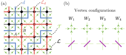
Figure 8: (a) Example of loop configuration $d$ (thick blue lines) on the dual lattice $\mathcal{D}$ such that $\mathcal{L}_{d}$ (thick red lines) is also a loop configuration. Black lines represent the original lattice $\mathcal{L}$. Black dots represent the sites where $s$ and $\tau$ spins live. Green lines represent the tilted lattice $\mathcal{T}$. Green arrows show one of the associated vertex configurations. (b) Each line segment diagonal in $\mathcal{T}$ (purple segments in the bottom line, which can be segments of either $d$ or $\mathcal{L}_{d}$) maps to the vertex configurations in the middle line with the corresponding weights $W_{i}$ ($1\leq i\leq 4$). Once a possible vertex is selected in one vertex, the other vertices are uniquely determined according to this assignment.

Let $\mathcal{T}$ be a $45^{\circ}$-tilted square lattice whose vertices pass across all the edges of $\mathcal{L}$. Let $A$ ($B$) be the sublattice of $\mathcal{T}$ that horizontal edges of $\mathcal{L}$ ($\mathcal{D}$) pass through. Now, $\mathcal{Z}$ can be mapped to a certain vertex model via the following weight assignment:

$$W_{1}^{A}=W_{2}^{A}=W_{3}^{B}=W_{4}^{B} =1,$$ (56)

$$W_{3}^{A}=W_{4}^{A}=W_{1}^{B}=W_{2}^{B} =\frac{R}{2-R},$$

where the superscripts denote the sublattices in $\mathcal{T}$, and the weights $W_{i}$ ($1\leq i\leq 4$) are assigned to the local vertices as shown in Fig. 8(b). (This mapping is one-to-two: two vertex configurations with opposite arrows map to the same $d$.) The weights Eq. (56) vary depending on the sublattice and hence define a “staggered vertex” model. When $R=1$, the staggeredness disappears, reducing the model to the “right-angle water” ice model [81]. [For a finite torus geometry, some loop configuration can lead to antiperiodic boundary conditions along the non-contractible loops of the torus, i.e., the arrows change their directions across these loops [80]. Since we are interested in the thermodynamic limit, we consider an infinite plane geometry and neglect such an issue below.]

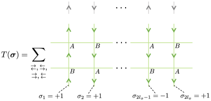
Figure 9: Transfer matrix element $T(\bm{\sigma})$ of the staggered vertex model. Gray arrows at the top show the fiducial antiferromagnetic arrow pattern, based on which variables $\bm{\sigma}=(\sigma_{i})_{i=1}^{2l_{x}}$ are defined. Each $T(\bm{\sigma})$ is a sum of the four terms corresponding to the four-row patterns $\begin{subarray}{c}\leftarrow\\[-10.00002pt] \rightarrow\end{subarray}$, $\begin{subarray}{c}\rightarrow\\[-10.00002pt] \leftarrow\end{subarray}$, $\begin{subarray}{c}\rightarrow\\[-10.00002pt] \rightarrow\end{subarray}$, and $\begin{subarray}{c}\leftarrow\\[-10.00002pt] \leftarrow\end{subarray}$.

The model Eq. (56) can be easily solved due to the non-reversing arrows along each line of $\mathcal{T}$ [see Fig. 8(a)]. Let’s first compute the transfer matrix of the model Eq. (56) in the diagonal direction of the original lattice $\mathcal{L}$, i.e., along the direction of the tilted lattice $\mathcal{T}$. Let’s suppose that $\mathcal{T}$ has a size $2l_{x}\times 2l_{y}$ for a while, and then take a limit $l_{x,y}\rightarrow\infty$ to compute physical quantities in an infinite plane geometry. Define variables $\bm{\sigma}=(\sigma_{i})_{i=1}^{2l_{x}}$ along the $l_{x}$-direction as follows (see Fig. 9): Consider a fiducial antiferromagnetic arrow pattern $\uparrow\downarrow\uparrow\downarrow\cdots$, which starts from a site in the $A$ sublattice. Define $\sigma_{i}=1$ ($-1$) if the vertical arrow of the $i$th site matches (mismatches) that of the fiducial pattern. Let’s also consider a small alternating electric field along the fiducial pattern, i.e., upward for the odd lines and downward for the even lines, so that the vertices with vertical arrows aligning with (against) the electric field gain an additional $\epsilon$ ($\epsilon^{-1}$) factor for some $\epsilon>1$. We consider this electric field to consider a spontaneous symmetry breaking, choosing one of the two vertical arrow patterns satisfying $O(\bm{\sigma})\equiv\sum_{i=1}^{2l_{x}}\sigma_{i}=\pm 2l_{x}$.

Let $r=R/(2-R)$ and $T$ be a transfer matrix corresponding to two rows, which involve four cases for their arrow directions: $\begin{subarray}{c}\leftarrow\\[-10.00002pt] \rightarrow\end{subarray}$, $\begin{subarray}{c}\rightarrow\\[-10.00002pt] \leftarrow\end{subarray}$, $\begin{subarray}{c}\rightarrow\\[-10.00002pt] \rightarrow\end{subarray}$, and $\begin{subarray}{c}\leftarrow\\[-10.00002pt] \leftarrow\end{subarray}$ (see Fig. 9). Due to the non-reversing arrows, we can write $T=\sum_{\bm{\sigma}}T(\bm{\sigma})|\bm{\sigma}\rangle\langle\bm{\sigma}|$ with $T(\bm{\sigma})=\prod_{i=1}^{2l_{x}}t(\sigma_{i})$, where $t(\sigma_{i})$ is a local weight for the $i$th column. One can compute $t(\sigma_{i})$ for the four cases as follows:

1. Case $\begin{subarray}{c}\leftarrow\\[-10.00002pt] \rightarrow\end{subarray}$:  $t(\sigma_{i})=\epsilon^{2\sigma_{i}}r^{1-\sigma_{i}}$

   • When $\sigma_{i}=1$ for odd $i$, $t(\sigma_{i})=W_{1}^{A}W_{4}^{B}=\epsilon^{2}$.

   • When $\sigma_{i}=1$ for even $i$, $t(\sigma_{i})=W_{3}^{B}W_{2}^{A}=\epsilon^{2}$.

   • When $\sigma_{i}=-1$ for odd $i$, $t(\sigma_{i})=W_{3}^{A}W_{2}^{B}=\epsilon^{-2}r^{2}$.

   • When $\sigma_{i}=-1$ for even $i$, $t(\sigma_{i})=W_{1}^{B}W_{4}^{A}=\epsilon^{-2}r^{2}$.

2. Case $\begin{subarray}{c}\rightarrow\\[-10.00002pt] \leftarrow\end{subarray}$:  $t(\sigma_{i})=\epsilon^{2\sigma_{i}}r^{1+\sigma_{i}}$

   • When $\sigma_{i}=1$ for odd $i$, $t(\sigma_{i})=W_{4}^{A}W_{1}^{B}=\epsilon^{2}r^{2}$.

   • When $\sigma_{i}=1$ for even $i$, $t(\sigma_{i})=W_{2}^{B}W_{3}^{A}=\epsilon^{2}r^{2}$.

   • When $\sigma_{i}=-1$ for odd $i$, $t(\sigma_{i})=W_{2}^{A}W_{3}^{B}=\epsilon^{-2}$.

   • When $\sigma_{i}=-1$ for even $i$, $t(\sigma_{i})=W_{4}^{B}W_{1}^{A}=\epsilon^{-2}$.

3. Case $\begin{subarray}{c}\rightarrow\\[-10.00002pt] \rightarrow\end{subarray}$:  $t(\sigma_{i})=\epsilon^{2\sigma_{i}}r$

   • When $\sigma_{i}=1$ for odd $i$, $t(\sigma_{i})=W_{1}^{A}W_{1}^{B}=\epsilon^{2}r$.

   • When $\sigma_{i}=1$ for even $i$, $t(\sigma_{i})=W_{3}^{B}W_{3}^{A}=\epsilon^{2}r$.

   • When $\sigma_{i}=-1$ for odd $i$, $t(\sigma_{i})=W_{3}^{A}W_{3}^{B}=\epsilon^{-2}r$.

   • When $\sigma_{i}=-1$ for even $i$, $t(\sigma_{i})=W_{1}^{B}W_{1}^{A}=\epsilon^{-2}r$.

4. Case $\begin{subarray}{c}\leftarrow\\[-10.00002pt] \leftarrow\end{subarray}$:  $t(\sigma_{i})=\epsilon^{2\sigma_{i}}r$

   • When $\sigma_{i}=1$ for odd $i$, $t(\sigma_{i})=W_{4}^{A}W_{4}^{B}=\epsilon^{2}r$.

   • When $\sigma_{i}=1$ for even $i$, $t(\sigma_{i})=W_{2}^{B}W_{2}^{A}=\epsilon^{2}r$.

   • When $\sigma_{i}=-1$ for odd $i$, $t(\sigma_{i})=W_{2}^{A}W_{2}^{B}=\epsilon^{-2}r$.

   • When $\sigma_{i}=-1$ for even $i$, $t(\sigma_{i})=W_{4}^{B}W_{4}^{A}=\epsilon^{-2}r$.

Combining all, we obtain

$$T(\bm{\sigma})=2\epsilon^{O(\bm{\sigma})}r^{2l_{x}}\left[1+\cosh\left(O(\bm{\sigma})\log r\right)\right].$$ (57)

Note that $T$ only depends on $O(\bm{\sigma})$, whose value takes even integers from $-2l_{x}$ to $2l_{x}$. Since $T(\bm{\sigma})$ is monotonic in $|O(\bm{\sigma})|$ when $\epsilon=1$, the correlation length is given by

$$\xi=-\frac{1}{\log\left(\frac{1+\cosh[2(l_{x}-1)\log r]}{1+\cosh[2l_{x}\log r]}\right)}\underset{l_{x}\rightarrow\infty}{\longrightarrow}-\frac{1}{2\log r},$$ (58)

which diverges as $[4(1-R)]^{-1}$ as $R\rightarrow 1$.

The order parameter $O=\langle O(\bm{\sigma})\rangle/(2l_{x})$ can be directly computed from Eq. (57). Consider first a case with $0\leq R<1$. It is straightforward to show that

$$O =\frac{\sum_{\bm{\sigma}}\frac{1}{2l_{x}}O(\bm{\sigma})T(\bm{\sigma})^{l_{y}}}{\sum_{\bm{\sigma}}T(\bm{\sigma})^{l_{y}}}$$ (59)

$$=\frac{\frac{1}{l_{x}}\sum_{p=-l_{x}}^{l_{x}}p\binom{2l_{x}}{l_{x}+p}\epsilon^{2l_{y}p}\left[1+\cosh\left(2p\log r\right)\right]^{l_{y}}}{\sum_{p=-l_{x}}^{l_{x}}\binom{2l_{x}}{l_{x}+p}\epsilon^{2l_{y}p}\left[1+\cosh\left(2p\log r\right)\right]^{l_{y}}},$$

where we have let $2p=O(\bm{\sigma})$. Since $\epsilon>1$, the expression $\epsilon^{2l_{y}p}\left[1+\cosh\left(2p\log r\right)\right]^{l_{y}}$ dominates at $p=l_{x}$ as $l_{y}\rightarrow\infty$. Therefore, we have

$$O \underset{l_{y}\rightarrow\infty}{\longrightarrow}\frac{\frac{1}{l_{x}}\cdot l_{x}\cdot\epsilon^{2l_{x}l_{y}}\left[1+\cosh\left(2l_{x}\log r\right)\right]^{l_{y}}}{\epsilon^{2l_{x}l_{y}}\left[1+\cosh\left(2l_{x}\log r\right)\right]^{l_{y}}}=1.$$ (60)

For the case of $R=1$, $T(\bm{\sigma})=4\epsilon^{O(\bm{\sigma})}$ and hence

$$O =\frac{\frac{1}{l_{x}}\sum_{p=-l_{x}}^{l_{x}}p\binom{2l_{x}}{l_{1}+p}\epsilon^{2l_{y}p}}{\sum_{p=-l_{x}}^{l_{x}}\binom{2l_{x}}{l_{x}+p}\epsilon^{2l_{y}p}}=\frac{\epsilon^{2l_{y}}-1}{\epsilon^{2l_{y}}+1}.$$ (61)

One can observe that $\lim_{\epsilon\rightarrow 1^{+}}\lim_{l_{x,y}\rightarrow\infty}O=1$, while $\lim_{l_{x,y}\rightarrow\infty}\lim_{\epsilon\rightarrow 1^{+}}O=0$. This is the spontaneous breaking of the symmetry that reverses the arrow directions. This behavior of the order parameter $O$ and the diverging correlation length at $R=1$ indicate that the model Eq. (56) does not undergo phase transition for $R<1$.

Now, we compute the anyon parameters for $R<1$, whose stat-mech expressions follow from Eq. (9):

$$\langle\!\langle I\bar{I}|e\bar{e}\rangle\!\rangle =\lim_{|i-j|\rightarrow\infty}\langle s_{i}s_{j}\rangle,$$ (62)

$$\langle\!\langle e\bar{I}|e\bar{I}\rangle\!\rangle =\lim_{i^{2}+j^{2}\rightarrow\infty}(-1)^{i+j}\langle\tau_{(0,0)}\tau_{(i,j)}\rangle,$$

$$\langle\!\langle I\bar{I}|m\bar{m}\rangle\!\rangle =\lim_{\tilde{i}^{2}+\tilde{j}^{2}\rightarrow\infty}(-1)^{\tilde{i}+\tilde{j}}\langle\mu_{(\tilde{0},\tilde{0})}^{\tau}\mu_{(\tilde{i},\tilde{j})}^{\tau}\rangle,$$

$$\langle\!\langle m\bar{I}|m\bar{I}\rangle\!\rangle =\lim_{|\tilde{i}-\tilde{j}|\rightarrow\infty}\langle\mu_{\tilde{i}}^{s}\mu_{\tilde{j}}^{s}\rangle,$$

[This differs from Eq. (16) since we have exchanged $s$ and $s\tau$ spins and then flipped the $\tau$ spins placed at site $(i,j)$ with $i+j$ odd.] Let’s first compute $\langle\tau_{(0,0)}\tau_{(i,j)}\rangle=\langle\prod_{e\in l}\tau_{v}\tau_{v^{\prime}}\rangle$, where $l$ is any string on the original lattice $\mathcal{L}$ connecting sites $(0,0)$ and $(i,j)$. From Eq. (54), we have $w_{e}\tau_{i}\tau_{j}=[2R/(2-R)]s_{v}s_{v^{\prime}}$ if $\tau_{v}\tau_{v^{\prime}}=-1$, and $-2$ otherwise. This corresponds to flipping $1$ to $-1$ in Eq. (56) for the vertices passing through edges $e\in l$. Suppose that $l$ is contained in $2q$ rows of $\mathcal{T}$ (see Fig. 10 for $q=2$). Then, since $|\bm{\sigma}_{0}\rangle$ with $\bm{\sigma}_{0}=(\sigma_{i}=1)_{i=1}^{2l_{x}}$ is a eigenvector of $T$ with a dominant eigenvalue, we can write $\langle\tau_{(0,0)}\tau_{(i,j)}\rangle=\langle\bm{\sigma}_{0}|(T^{q})_{l}|\bm{\sigma}_{0}\rangle/\langle\bm{\sigma}_{0}|T^{q}|\bm{\sigma}_{0}\rangle$ as $l_{y}\rightarrow\infty$, where $(T^{q})_{l}$ is the same as $T^{q}$ except for flipping $1$ to $-1$ in Eq. (56) for the vertices passing through the intersections between $l$ and loops $d$ on dual lattice $\mathcal{D}$. Now, as $l_{x}\rightarrow\infty$, one can easily see that only the loop pattern full of $d$ (see Fig. 10) survives (other patterns give powers of $x^{2l_{x}}$, which vanish as $l_{x}\rightarrow\infty$). Since $l$ intersects with this loop pattern $i+j$ times, one get $\langle\bm{\sigma}_{0}|(T^{q})_{l}|\bm{\sigma}_{0}\rangle=(-1)^{i+j}\langle\bm{\sigma}_{0}|T^{q}|\bm{\sigma}_{0}\rangle$ and therefore

$$\langle\!\langle e\bar{I}|e\bar{I}\rangle\!\rangle=\lim_{i^{2}+j^{2}\rightarrow\infty}(-1)^{i+j}\langle\tau_{(0,0)}\tau_{(i,j)}\rangle=1.$$ (63)

Following a similar argument, one can see that $\langle\mu_{\tilde{i}}^{s}\mu_{\tilde{j}}^{s}\rangle=\langle\bm{\sigma}_{0}|(T^{q})_{\tilde{l}}|\bm{\sigma}_{0}\rangle/\langle\bm{\sigma}_{0}|T^{q}|\bm{\sigma}_{0}\rangle$ as $l_{y}\rightarrow\infty$, where $\tilde{l}$ is a string on the dual lattice $\mathcal{D}$ connecting sites $\tilde{i}$ and $\tilde{j}$, and $(T^{q})_{\tilde{l}}$ is the same as $T^{q}$ except for flipping $r$ to $-r$ in Eq. (56) for the vertices passing through edges $e\in\tilde{l}$. Again, the loop pattern shown in Fig. 10 survives under the limit $l_{x}\rightarrow\infty$, yielding $\langle\bm{\sigma}_{0}|(T^{q})_{\tilde{l}}|\bm{\sigma}_{0}\rangle=\langle\bm{\sigma}_{0}|T^{q}|\bm{\sigma}_{0}\rangle$ and hence

$$\langle\!\langle m\bar{I}|m\bar{I}\rangle\!\rangle=\lim_{|i-j|\rightarrow\infty}\langle\mu_{\tilde{i}}^{s}\mu_{\tilde{j}}^{s}\rangle=1.$$ (64)

One can also show that the fermion condensation parameter $\langle\!\langle f\bar{I}|f\bar{I}\rangle\!\rangle=(-1)^{i+j}\langle\tau_{(0,0)}\mu_{(\tilde{0},\tilde{0})}^{s}\tau_{(i,j)}\mu_{(\tilde{i},\tilde{j})}^{s}\rangle$ converges to one in the same manner.

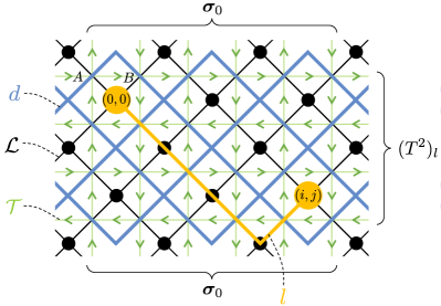
Figure 10: Modified transfer matrix element $\langle\bm{\sigma}_{0}|(T^{q})_{l}|\bm{\sigma}_{0}\rangle$ with $q=2$ appearing in the computation of $\langle\tau_{(0,0)}\tau_{(i,j)}\rangle$ in the staggered vertex model Eq. (56). The dominant loop configuration that survives under the limit $l_{x}\rightarrow\infty$ (blue loops) and the corresponding arrow pattern are displayed. Vertices where the yellow string passes through have flipped vertex weight when it intersects with $d$, yielding a $(-1)^{i+j}$ factor.

For the anyon condensation parameters, one can borrow the theorem in Ref. [82] stating that order and disorder parameters of Ising symmetric system with finite correlation length cannot be nonzero simultaneously. Since the correlation length Eq. (58) is finite for $R<1$ and the disorder parameters Eqs. (63) and (64) are finite, we can conclude that the corresponding order parameters must vanish, i.e., $\langle\!\langle I\bar{I}|e\bar{e}\rangle\!\rangle=\langle\!\langle m\bar{I}|m\bar{I}\rangle\!\rangle=0$.

To sum up, we have shown that $e$ and $m$ anyons are deconfined and $e\bar{e}$ and $m\bar{m}$ anyons are not condensed for all $R<1$. Along with the analysis of correlation length and order parameter $O$, it follows that the staggered vertex model does not undergo phase transition for $R<1$.

Appendix C Details on Amplitude Damping Noise

In this appendix, we elaborate on the details of the mapping to the stat-mech model discussed in Section. IV. We start by computing $\mathbb{E}_{\mathrm{amp}}^{\dagger}\mathbb{E}_{\mathrm{amp}}$ for the amplitude damping channel. From $\mathbb{E}_{e}=K_{0,e}\otimes\bar{K}_{0,e}+K_{1,e}\otimes\bar{K}_{1,e}$, one can easily show that

$$\mathbb{E}^{\dagger}\mathbb{E}\propto\prod_{e}\Bigg{[}1+\frac{\gamma(1-\gamma)}{\gamma^{2}-2\gamma+2}(Z_{e}+\bar{Z}_{e})+\frac{1}{\gamma^{2}-2\gamma+2}\left(\gamma^{2}Z_{e}\bar{Z}_{e}+\gamma X_{e}\bar{X}_{e}-\gamma Y_{e}\bar{Y}_{e}\right)\Bigg{]}.$$ (65)

From Eq. (4) and the identities $X_{e}|z_{e}\rangle=|{-}z_{e}\rangle$, $Y_{e}|z_{e}\rangle=i^{z_{e}}|{-}z_{e}\rangle$, and $Z_{e}|z_{e}\rangle=z_{e}|z_{e}\rangle$, it follows that $\mathrm{Tr}[\rho_{D}^{2}]=\langle\!\langle\rho_{0}|\mathbb{E}_{\mathrm{amp}}^{\dagger}\mathbb{E}_{\mathrm{amp}}|\rho_{0}\rangle\!\rangle\propto\sum_{\mathbf{x}_{v},\bar{\mathbf{x}}_{v},\mathbf{t}_{v},\bar{\mathbf{t}}_{v}}\prod_{e}\omega_{e}$, where

$$\omega_{e} =\sum_{z_{e},\bar{z}_{e}=\pm 1}(1+z_{e}t_{v}t_{v^{\prime}})(1+\bar{z}_{e}\bar{t}_{v}\bar{t}_{v^{\prime}})$$

$$\hskip 15.0pt\times\left[\left(1+\frac{\gamma^{2}z_{e}\bar{z}_{e}+\gamma(1-\gamma)(z_{e}+\bar{z}_{e})}{\gamma^{2}-2\gamma+2}\right)(1+z_{e}x_{v}x_{v^{\prime}})(1+\bar{z}_{e}\bar{x}_{v}\bar{x}_{v^{\prime}})+\frac{\gamma(1-i^{-z_{e}-\bar{z}_{e}})}{\gamma^{2}-2\gamma+2}(1-z_{e}x_{v}x_{v^{\prime}})(1-\bar{z}_{e}\bar{x}_{v}\bar{x}_{v^{\prime}})\right]$$

$$\propto 1+x_{v}x_{v^{\prime}}\bar{x}_{v}\bar{x}_{v^{\prime}}t_{v}t_{v^{\prime}}\bar{t}_{v}\bar{t}_{v^{\prime}}+\frac{\gamma^{2}-3\gamma+2}{\gamma^{2}-\gamma+2}(x_{v}x_{v^{\prime}}t_{v}t_{v^{\prime}}+\bar{x}_{v}\bar{x}_{v^{\prime}}\bar{t}_{v}\bar{t}_{v^{\prime}})+\frac{\gamma(1+\gamma)}{\gamma^{2}-\gamma+2}(x_{v}x_{v^{\prime}}\bar{x}_{v}\bar{x}_{v^{\prime}}+t_{v}t_{v^{\prime}}\bar{t}_{v}\bar{t}_{v^{\prime}})$$ (66)

$$\hskip 12.0pt+\frac{\gamma(1-\gamma)}{\gamma^{2}-\gamma+2}(x_{v}x_{v^{\prime}}+\bar{x}_{v}\bar{x}_{v^{\prime}}+t_{v}t_{v^{\prime}}+\bar{t}_{v}\bar{t}_{v^{\prime}}-x_{v}x_{v^{\prime}}\bar{t}_{v}\bar{t}_{v^{\prime}}-\bar{x}_{v}\bar{x}_{v^{\prime}}t_{v}t_{v^{\prime}}$$

$$\hskip 135.0pt+x_{v}x_{v^{\prime}}\bar{x}_{v}\bar{x}_{v^{\prime}}t_{v}t_{v^{\prime}}+x_{v}x_{v^{\prime}}t_{v}t_{v^{\prime}}\bar{t}_{v}\bar{t}_{v^{\prime}}+x_{v}x_{v^{\prime}}\bar{x}_{v}\bar{x}_{v^{\prime}}\bar{t}_{v}\bar{t}_{v^{\prime}}+\bar{x}_{v}\bar{x}_{v^{\prime}}t_{v}t_{v^{\prime}}\bar{t}_{v}\bar{t}_{v^{\prime}}).$$

Since Eq. (C) obeys $\omega_{e}(x_{v}x_{v^{\prime}}\bar{x}_{v}\bar{x}_{v^{\prime}}t_{v}t_{v^{\prime}}\bar{t}_{v}\bar{t}_{v^{\prime}})=\omega_{e}$, we can let $\bar{t}_{v}\bar{t}_{v^{\prime}}=x_{v}x_{v^{\prime}}\bar{x}_{v}\bar{x}_{v^{\prime}}t_{v}t_{v^{\prime}}$ and obtain

$$\omega_{e} \propto 1+\frac{\gamma(1+\gamma)}{\gamma^{2}-\gamma+2}CA-\frac{\gamma(1-\gamma)}{\gamma^{2}-\gamma+2}BC+\frac{\gamma^{2}-3\gamma+2}{\gamma^{2}-\gamma+2}AB+\frac{\gamma(1-\gamma)}{\gamma^{2}-\gamma+2}(A+B+C+ABC),$$ (67)

where we simplified the notations as $A\equiv x_{v}x_{v^{\prime}}$, $B=t_{v}t_{v^{\prime}}$, and $C\equiv\bar{x}_{v}\bar{x}_{v^{\prime}}$.

We argue that we can neglect the last term in Eq. (67) proportional to $A+B+C+ABC$. When $\gamma=0$ or $1$, the last term of Eq. (67) vanishes trivially. Now, consider the case $0<\gamma<1$. Let’s first represent Eq. (67) as a local Boltzmann weight. To this end, it is convenient to consider the cases with $B=\pm C$ separately.

1. When $B=C$, Eq. (67) reduces to

   $$\omega_{e}\propto\frac{2(\gamma^{2}-\gamma+1)}{\gamma^{2}-\gamma+2}\left[1+AB+\frac{\gamma(1-\gamma)}{\gamma^{2}-\gamma+1}(A+B)\right]=\frac{2(\gamma^{2}-\gamma+1)}{\gamma^{2}-\gamma+2}\frac{\mathrm{sech}^{2}(c_{1})\mathrm{sech}(c_{2})}{1+\tanh^{2}(c_{1})\tanh(c_{2})}e^{c_{1}(A+B)+c_{2}AB},$$ (68)

   where $c_{1}=\tanh^{-1}\left[(\gamma^{2}-\gamma+1-\sqrt{2\gamma^{2}-2\gamma+1})/\gamma(1-\gamma)\right]<\infty$ and $c_{2}=\infty$. For a while, we formally regard $c_{2}$ as a large number.

2. When $B=-C$, Eq. (67) reduces to

   $$\omega_{e}\propto\frac{2}{\gamma^{2}-\gamma+2}\left[1-(1-2\gamma)AB\right]=\frac{4\sqrt{\gamma(1-\gamma)}}{\gamma^{2}-\gamma+2}e^{-c_{3}AB},$$ (69)

   where $c_{3}=\tanh^{-1}(1-2\gamma)<\infty$.

Define

$$c_{4}=\log\left(\frac{\gamma^{2}-\gamma+1}{2\sqrt{\gamma(1-\gamma)}}\frac{\mathrm{sech}^{2}c_{1}\,\mathrm{sech}c_{2}}{1+\tanh^{2}c_{1}\tanh c_{2}}\right).$$ (70)

Since $e^{\frac{c_{4}}{2}BC}$ becomes the prefactors of Eqs. (68) and (69) (up to some common prefactor) for $B=\pm C$, respectively, we can combine these two cases using projectors $(1\pm BC)/2$ as

$$\!\omega_{e} \propto e^{\frac{c_{4}}{2}BC}e^{\frac{1+BC}{2}[c_{1}(A+B)+c_{2}AB]}e^{-\frac{1-BC}{2}c_{3}AB}=\exp\left[\Omega_{0}(A+B+C+ABC)+\Omega_{AB}AB+\Omega_{BC}BC+\Omega_{CA}CA\right],$$ (71)

where $\Omega_{0}=c_{1}/2$, $\Omega_{AB}=(c_{2}-c_{3})/2$, $\Omega_{BC}=c_{4}/2$, and $\Omega_{CA}=(c_{2}+c_{3})/2$. Notice that $\Omega_{0}$ is always finite, while $\Omega_{AB},\Omega_{CA}\sim c_{2}/2$ and $\Omega_{BC}\sim-c_{2}/2$ as we take $c_{2}\rightarrow\infty$. Therefore, for all $0<\gamma<1$, the phase of the model is determined by the competition between the diverging coupling constants $\Omega_{AB}$, $\Omega_{BC}$, and $\Omega_{CA}$ and the effect of $\Omega_{0}$ is negligible. (The diverging coupling constants cannot cancel off each other.) Thus, neglecting $\Omega_{0}$ in Eq. (71) should not affect the phase of the model. Since the last term in Eq. (67) cannot appear when there is no $\Omega_{0}(A+B+C+ABC)$ term in Eq. (71), we can conclude that we can safely drop the last term in Eq. (67) without altering the phase of the model. It then follows that

$$\omega_{e}\propto 1+\frac{\gamma(1+\gamma)}{\gamma^{2}-\gamma+2}CA-\frac{\gamma(1-\gamma)}{\gamma^{2}-\gamma+2}BC+\frac{\gamma^{2}-3\gamma+2}{\gamma^{2}-\gamma+2}AB,$$ (72)

which is the weight $\omega_{e}\propto 1+J_{+}s_{v}s_{v^{\prime}}-J_{-}\tau_{v}\tau_{v^{\prime}}+Ks_{v}s_{v^{\prime}}\tau_{v}\tau_{v^{\prime}}$ with $J_{\pm}$ and $K$ given by Eq. (23) upon defining new Ising variables $s_{v}=x_{v}\bar{x}_{v}$ and $\tau_{v}=\bar{x}_{v}t_{v}$. Expressing this in the form of $\omega_{e}\propto e^{\mathcal{J}_{1}s_{v}s_{v^{\prime}}+\mathcal{J}_{2}\tau_{v}\tau_{v^{\prime}}+\mathcal{K}s_{v}s_{v^{\prime}}\tau_{v}\tau_{v^{\prime}}}$, it must be

$$\frac{\tanh(\mathcal{J}_{1})+\tanh(\mathcal{J}_{2})\tanh(\mathcal{K})}{1+\tanh(\mathcal{J}_{1})\tanh(\mathcal{J}_{2})\tanh(\mathcal{K})} =J_{+},$$ (73)

$$\frac{\tanh(\mathcal{J}_{2})+\tanh(\mathcal{J}_{1})\tanh(\mathcal{K})}{1+\tanh(\mathcal{J}_{1})\tanh(\mathcal{J}_{2})\tanh(\mathcal{K})} =J_{-},$$

$$\frac{\tanh(K)+\tanh(\mathcal{J}_{1})\tanh(\mathcal{J}_{2})}{1+\tanh(\mathcal{J}_{1})\tanh(\mathcal{J}_{2})\tanh(\mathcal{K})} =K.$$

We have numerically checked that for $\gamma\in(0,1)$, the solutions of Eq. (73) are all finite reals. For $\gamma=0$ ($1$), one gets $\mathcal{J}_{1}=\mathcal{J}_{2}=0$ and $\mathcal{K}=\infty$ ($\mathcal{J}_{1}=\infty$ and $\mathcal{J}_{2}=\mathcal{K}=0$). Therefore, the mixed-state phase of the TC under amplitude damping noise is associated with the anisotropic AT model (with $\mathcal{J}_{2}\leq 0$).

References

- Wen [2004] X.-G. Wen, Quantum field theory of many-body systems: From the origin of sound to an origin of light and electrons (OUP Oxford, 2004).
- Sachdev [2023] S. Sachdev, Quantum Phases of Matter (Cambridge University Press, 2023).
- Kitaev [2003] A. Y. Kitaev, Annals of physics 303, 2 (2003).
- Dennis et al. [2002] E. Dennis, A. Kitaev, A. Landahl, and J. Preskill, Journal of Mathematical Physics 43, 4452 (2002).
- Semeghini et al. [2021] G. Semeghini, H. Levine, A. Keesling, S. Ebadi, T. T. Wang, D. Bluvstein, R. Verresen, H. Pichler, M. Kalinowski, R. Samajdar, et al., Science 374, 1242 (2021).
- Satzinger et al. [2021] K. Satzinger, Y.-J. Liu, A. Smith, C. Knapp, M. Newman, C. Jones, Z. Chen, C. Quintana, X. Mi, A. Dunsworth, et al., Science 374, 1237 (2021).
- Foss-Feig et al. [2023] M. Foss-Feig, A. Tikku, T. Lu, K. Mayer, M. Iqbal, T. Gatterman, J. Gerber, K. Gilmore, D. Gresh, A. Hankin, et al., arXiv preprint arXiv:2302.03029 (2023).
- Iqbal et al. [2024a] M. Iqbal, N. Tantivasadakarn, T. M. Gatterman, J. A. Gerber, K. Gilmore, D. Gresh, A. Hankin, N. Hewitt, C. V. Horst, M. Matheny, et al., Communications Physics 7, 205 (2024a).
- Iqbal et al. [2024b] M. Iqbal, N. Tantivasadakarn, R. Verresen, S. L. Campbell, J. M. Dreiling, C. Figgatt, J. P. Gaebler, J. Johansen, M. Mills, S. A. Moses, et al., Nature 626, 505 (2024b).
- Xu et al. [2024] S. Xu, Z.-Z. Sun, K. Wang, H. Li, Z. Zhu, H. Dong, J. Deng, X. Zhang, J. Chen, Y. Wu, et al., Nature Physics , 1 (2024).
- Minev et al. [2024] Z. K. Minev, K. Najafi, S. Majumder, J. Wang, A. Stern, E.-A. Kim, C.-M. Jian, and G. Zhu, arXiv preprint arXiv:2406.12820 (2024).
- Preskill [2018] J. Preskill, Quantum 2, 79 (2018).
- de Groot et al. [2022] C. de Groot, A. Turzillo, and N. Schuch, Quantum 6, 856 (2022).
- Lee et al. [2022] J. Y. Lee, Y.-Z. You, and C. Xu, arXiv preprint arXiv:2210.16323 (2022).
- Bao et al. [2023] Y. Bao, R. Fan, A. Vishwanath, and E. Altman, arXiv preprint arXiv:2301.05687 (2023).
- Lee et al. [2023] J. Y. Lee, C.-M. Jian, and C. Xu, PRX Quantum 4, 030317 (2023).
- Fan et al. [2024] R. Fan, Y. Bao, E. Altman, and A. Vishwanath, PRX Quantum 5, 020343 (2024).
- Lee [2024] J. Y. Lee, arXiv preprint arXiv:2402.16937 (2024).
- Niwa and Lee [2024] R. Niwa and J. Y. Lee, arXiv preprint arXiv:2407.02564 (2024).
- Ma and Wang [2023] R. Ma and C. Wang, Phys. Rev. X 13, 031016 (2023).
- Sang et al. [2024] S. Sang, Y. Zou, and T. H. Hsieh, Physical Review X 14, 031044 (2024).
- Sang and Hsieh [2024] S. Sang and T. H. Hsieh, arXiv preprint arXiv:2404.07251 (2024).
- Zou et al. [2023] Y. Zou, S. Sang, and T. H. Hsieh, Phys. Rev. Lett. 130, 250403 (2023).
- Lu et al. [2023] T.-C. Lu, Z. Zhang, S. Vijay, and T. H. Hsieh, PRX Quantum 4, 030318 (2023).
- Guo and Ashida [2024] Y. Guo and Y. Ashida, Phys. Rev. B 109, 195420 (2024).
- Ma et al. [2023] R. Ma, J.-H. Zhang, Z. Bi, M. Cheng, and C. Wang, arXiv preprint arXiv:2305.16399 (2023).
- Ma and Turzillo [2024] R. Ma and A. Turzillo, arXiv preprint arXiv:2403.13280 (2024).
- Chen and Grover [2024a] Y.-H. Chen and T. Grover, PRX Quantum 5, 030310 (2024a).
- Chen and Grover [2024b] Y.-H. Chen and T. Grover, Phys. Rev. Lett. 132, 170602 (2024b).
- Chen and Grover [2024c] Y.-H. Chen and T. Grover, Physical Review B 110, 125152 (2024c).
- Myerson-Jain et al. [2023] N. Myerson-Jain, T. L. Hughes, and C. Xu, arXiv preprint arXiv:2312.04638 (2023).
- Wang et al. [2023] Z. Wang, Z. Wu, and Z. Wang, arXiv preprint arXiv:2307.13758 (2023).
- Su et al. [2024a] K. Su, N. Myerson-Jain, C. Wang, C.-M. Jian, and C. Xu, Physical Review Letters 132, 200402 (2024a).
- Su et al. [2024b] K. Su, N. Myerson-Jain, and C. Xu, Phys. Rev. B 109, 035146 (2024b).
- Lyons [2024] A. Lyons, arXiv preprint arXiv:2403.03955 (2024).
- Su et al. [2024c] K. Su, Z. Yang, and C.-M. Jian, Physical Review B 110, 085158 (2024c).
- Li and Mong [2024] Z. Li and R. S. Mong, arXiv preprint arXiv:2402.09516 (2024).
- Zhang et al. [2024] Z. Zhang, U. Agrawal, and S. Vijay, arXiv preprint arXiv:2405.05965 (2024).
- Lu [2024] T.-C. Lu, Physical Review B 110, 125145 (2024).
- Sohal and Prem [2024] R. Sohal and A. Prem, arXiv preprint arXiv:2403.13879 (2024).
- Ellison and Cheng [2024] T. Ellison and M. Cheng, arXiv preprint arXiv:2405.02390 (2024).
- Lessa et al. [2024a] L. A. Lessa, M. Cheng, and C. Wang, arXiv preprint arXiv:2401.17357 (2024a).
- Lessa et al. [2024b] L. A. Lessa, R. Ma, J.-H. Zhang, Z. Bi, M. Cheng, and C. Wang, arXiv preprint arXiv:2405.03639 (2024b).
- Sala et al. [2024] P. Sala, S. Gopalakrishnan, M. Oshikawa, and Y. You, Physical Review B 110, 155150 (2024).
- Hauser et al. [2024] J. Hauser, Y. Bao, S. Sang, A. Lavasani, U. Agrawal, and M. Fisher, arXiv preprint arXiv:2407.07882 (2024).
- Eckstein et al. [2024] F. Eckstein, B. Han, S. Trebst, and G.-Y. Zhu, PRX Quantum 5, 040313 (2024).
- Kueng et al. [2016] R. Kueng, D. M. Long, A. C. Doherty, and S. T. Flammia, Phys. Rev. Lett. 117, 170502 (2016).
- Greenbaum and Dutton [2017] D. Greenbaum and Z. Dutton, Quantum Science and Technology 3, 015007 (2017).
- Bravyi et al. [2018] S. Bravyi, M. Englbrecht, R. König, and N. Peard, npj Quantum Information 4, 55 (2018).
- Venn et al. [2023] F. Venn, J. Behrends, and B. Béri, Phys. Rev. Lett. 131, 060603 (2023).
- Chirolli and Burkard [2008] L. Chirolli and G. Burkard, Advances in Physics 57, 225 (2008).
- Haegeman et al. [2015] J. Haegeman, V. Zauner, N. Schuch, and F. Verstraete, Nature communications 6, 8284 (2015).
- Duivenvoorden et al. [2017] K. Duivenvoorden, M. Iqbal, J. Haegeman, F. Verstraete, and N. Schuch, Phys. Rev. B 95, 235119 (2017).
- Schumacher and Nielsen [1996] B. Schumacher and M. A. Nielsen, Phys. Rev. A 54, 2629 (1996).
- Lloyd [1997] S. Lloyd, Phys. Rev. A 55, 1613 (1997).
- Briegel and Raussendorf [2001] H. J. Briegel and R. Raussendorf, Phys. Rev. Lett. 86, 910 (2001).
- Raussendorf et al. [2005] R. Raussendorf, S. Bravyi, and J. Harrington, Phys. Rev. A 71, 062313 (2005).
- Jamiołkowski [1972] A. Jamiołkowski, Reports on mathematical physics 3, 275 (1972).
- Choi [1975] M.-D. Choi, Linear algebra and its applications 10, 285 (1975).
- Bais and Slingerland [2009] F. A. Bais and J. K. Slingerland, Phys. Rev. B 79, 045316 (2009).
- Burnell [2018] F. J. Burnell, Annual Review of Condensed Matter Physics 9, 307 (2018).
- Umegaki [1962] H. Umegaki, in Kodai Mathematical Seminar Reports, Vol. 14 (Department of Mathematics, Tokyo Institute of Technology, 1962) pp. 59–85.
- Petz [1986] D. Petz, Reports on mathematical physics 23, 57 (1986).
- Kadanoff and Ceva [1971] L. P. Kadanoff and H. Ceva, Phys. Rev. B 3, 3918 (1971).
- Nishino [1995] T. Nishino, Journal of the Physical Society of Japan 64, 3598 (1995).
- Nishino and Okunishi [1996] T. Nishino and K. Okunishi, Journal of the Physical Society of Japan 65, 891 (1996).
- Fishman et al. [2018] M. T. Fishman, L. Vanderstraeten, V. Zauner-Stauber, J. Haegeman, and F. Verstraete, Phys. Rev. B 98, 235148 (2018).
- Pollmann et al. [2009] F. Pollmann, S. Mukerjee, A. M. Turner, and J. E. Moore, Phys. Rev. Lett. 102, 255701 (2009).
- Baxter [2007] R. J. Baxter, Exactly solved models in statistical mechanics (Courier Corporation, 2007).
- Onsager [1944] L. Onsager, Phys. Rev. 65, 117 (1944).
- Kramers and Wannier [1941] H. A. Kramers and G. H. Wannier, Phys. Rev. 60, 252 (1941).
- Tuckett et al. [2019] D. K. Tuckett, A. S. Darmawan, C. T. Chubb, S. Bravyi, S. D. Bartlett, and S. T. Flammia, Phys. Rev. X 9, 041031 (2019).
- Tuckett et al. [2018] D. K. Tuckett, S. D. Bartlett, and S. T. Flammia, Phys. Rev. Lett. 120, 050505 (2018).
- Chubb and Flammia [2021] C. T. Chubb and S. T. Flammia, Annales de l’Institut Henri Poincaré D 8, 269 (2021).
- Botzung et al. [2023] T. Botzung, M. Buchhold, S. Diehl, and M. Müller, arXiv preprint arXiv:2311.14338 (2023).
- Lee and Yoshida [2024] D. Lee and B. Yoshida, arXiv preprint arXiv:2402.00145 (2024).
- Krčmár et al. [2022] R. Krčmár, A. Gendiar, and L. Šamaj, Phys. Rev. E 105, 054112 (2022).
- Behrends and Béri [2024] J. Behrends and B. Béri, arXiv preprint arXiv:2410.22436 (2024).
- Nienhuis [1984] B. Nienhuis, Journal of Statistical Physics 34, 731 (1984).
- Saleur [1987] H. Saleur, Journal of Physics A: Mathematical and General 20, L1127 (1987).
- Ziman [1979] J. M. Ziman, Models of disorder: the theoretical physics of homogeneously disordered systems (Cambridge university press, 1979).
- Levin [2020] M. Levin, Communications in Mathematical Physics 378, 1081 (2020).