Infinitely fast critical dynamics: Teleportation through temporal rare regions in monitored quantum circuits

Abstract

We consider measurement-induced phase transitions in monitored quantum circuits with a measurement rate that fluctuates in time. The spatially correlated fluctuations in the measurement rate disrupt the volume-law phase for low measurement rates; at a critical measurement rate, they give rise to an entanglement phase transition with “ultrafast” dynamics, i.e., spacetime ($x,t$) scaling $\log x\sim t^{\psi_{\tau}}$. The ultrafast dynamics at the critical point can be viewed as a spacetime-rotated version of an infinite-randomness critical point; despite the spatial locality of the dynamics, ultrafast information propagation is possible because of measurement-induced quantum teleportation. We identify temporal Griffiths phases on either side of this critical point. We provide a physical interpretation of these phases, and support it with extensive numerical simulations of information propagation and entanglement dynamics in stabilizer circuits.

I Introduction

Enriching quantum dynamics beyond the unitary limit through the use of measurements has demonstrated significant potential for quantum state preparation and quantum error correction. Measurements have two qualitatively different effects on the dynamics of entanglement in quantum many-body systems: measuring a subsystem to be in a unique pure state disentangles it; however, such measurements can also teleport information in the rest of the system, transmuting short-range entanglement into long-range entanglement [1, 2, 3]. These effects underlie two remarkable information-theoretic phase transitions that were discovered in the past few years. The first is the measurement-induced phase transition (MIPT) in the entanglement structure of monitored quantum circuits, driven by the competition between the entangling power of unitary dynamics and the disentangling effects of measurements [4, 5, 6, 7]; the second is the teleportation transition, at which measuring all but two well-separated spins in a many-body system creates entanglement between the remaining spins [8]. Because measurements can teleport information, monitored circuits do not have strict causal light-cones. This apparent lack of causality is consistent with the laws of physics because to send signals through teleportation one needs to perform classical communication, which cannot be superluminal. It was recently shown [9] that certain measures of quantum information propagate superluminally (with the dynamical scaling $x\sim t^{3/2}$) in monitored circuits in the low-measurement phase. Nevertheless, the critical point at the “standard” MIPT is governed by a conformal field theory, with emergent isotropic spacetime scaling (i.e. it has a dynamical exponent $z$ that relates space and time scaling $t\sim x^{z}$ with $z=1$) [10, 3, 11].

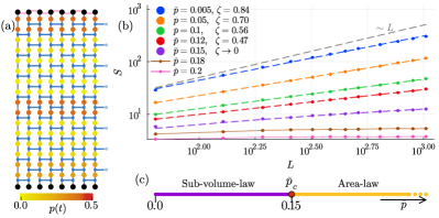
(a)

(b)

(c)

Figure 1: (a) Graphical depiction of a brickwork quantum circuit with temporal randomness in the measurement rate. The blue lines mark the two-qubit Clifford gates, while the projective measurements operating between them follow a time-dependent measurement rate $p(t)$ denoted by the different colors. (b) The half-cut bipartite entanglement entropy with periodic boundary conditions at different values of $\bar{p}$ grows as $S\sim L^{\zeta}$ with $\zeta(\bar{p})<1$ for $0<\bar{p}<\bar{p}_{c}$, obeying a sub-volume-law behavior. (c) The phase diagram of the temporally random quantum circuit.

In this work, we leverage the teleporting power of measurements to create a critical point that strongly deviates from the relativistic scaling, with instead a vanishing dynamical exponent $z\to 0$, which we will term ultrafast dynamical scaling. The model we consider consists of a random quantum circuit subject to measurements occurring at a rate that fluctuates in time, but in a globally spatially correlated way. In particular, therefore, the actual dynamics is local in spacetime: the only nonlocality comes from global correlations of the measurement rate and from the inherent nonlocality of quantum teleportation. This type of criticality is qualitatively different from standard quantum criticality: temporal randomness lacks a natural physical interpretation in ground-state quantum criticality; considering real-time dynamics opens the door to new types of critical phenomena.

The setup we are considering can be regarded as a spacetime-rotated version of a more standard infinite-randomness MIPT that was studied in [12]. In that work, measurement rates varied in space but not in time, giving rise to activated $z\to\infty$ critical dynamical scaling. Naively, interchanging the roles of space and time maps the $z\to\infty$ critical point to a $z\to 0$ critical point. However, as we will discuss, quantities like entanglement and mutual information do not map to natural observables under spacetime rotation; therefore, these quantities exhibit unusual features at the ultrafast critical point that have no direct analog in the spacetime-rotated version. In the bulk of the present work we characterize the properties of this critical point.

In addition to unusual critical behavior, this correlated-measurement model has unusual entanglement properties at low measurement rate. In general, one would expect entanglement to grow to a volume law in the low-measurement regime, as it does in an unmonitored chaotic system [13, 14, 15]. Instead, we find that temporal strips of high measurement rate are able to interrupt the growth of entanglement, so the steady state entanglement scales as a continuously varying power of subsystem size. By analogy with the infinite-randomness problem, one expects Griffiths phases near the MIPT; here, however, one enters a type of temporal Griffiths phase for any small nonzero measurement rate. This “interrupted volume law” phase has other surprising features: for example, the entanglement across a given cut has temporal fluctuations that are of the same magnitude as its average value.

For critical points with spatial quenched randomness, the Harris and the Chayes-Chayes-Fisher-Spencer (CCFS) bound on the correlation length exponent is $\nu\geq 2/d$ [16, 17, 18, 19]. Our work extends this notion to critical points with spatially uniform temporal randomness, with the observation that our estimates for the critical exponent for the correlation time $\xi_{\tau}\sim(\bar{p}-\bar{p}_{c})^{-\nu_{\tau}}$ saturates a putative temporal Harris/CCFS bound [33]

$$\nu_{\tau}\geq 2.$$ (1)

This paper is organized as follows: In Section II, we present the model under investigation: hybrid quantum circuits with temporally random measurement rates. We also detail physical probes employed to identify and characterize the distinct phases and associated phase transition. Moreover, we propose an ultrafast space-time scaling ansatz characterized by activated scaling and a vanishing dynamical exponent $z\rightarrow 0$ that governs the critical dynamics close to the MIPT. In Section III, we detail our numerical results: i) We report unconventional scaling properties of the entangling and area law phases, in the respective limits of strong and weak average measurement rates. ii) We conduct a careful analysis of the emergent universal critical properties of the MIPT, demonstrating an ultrafast dynamical scaling and numerical estimation of the associated critical exponents. iii) We examine the signatures of our findings in the context of information propagation and compare our results with the conventional relativistic MIPT and the ultraslow infinite-randomness fixed point in the presence of quenched randomness. Section IV summarizes our results, discusses their broader implications, and highlights future research directions.

II Monitored quantum circuit with temporal randomness

II.1 Model

To construct the model, we start from the previously-studied model with quenched randomness in the measurement rates  [12]. That model had random 2-qubit stabilizer gates with local random projective measurements in the computational basis with local measurement rates $p(x)$ that are static in time and only random in space. We then apply a spacetime rotation to the pattern of measurement rates ($x\rightarrow t$ and $t\rightarrow-x$), which yields measurement rates that are now uniform in space but random in time, $p(x)\rightarrow p(t)$, as depicted in Fig. 1a. This is not a full rotation of the previous model, because we are not rotating the gates. We note that we could, in principle, take dual-unitary Clifford gates [20, 21] that are in the same universality class as random Cliffords [11, 22, 23], and they would be invariant under this rotation. So we expect that in their bulks these two models related by this spacetime rotation are in the same universality class governed by an infinite randomness fixed point. The rare regions in space that dominate the dynamics in the infinite-randomness fixed point now become rare regions in time, and below we unveil unique aspects of such temporal Griffith effects. Relatedly, temporal Griffiths phases were recently reported in the context of decodable phases of error correction schemes in the presence of non-uniform noise rates [24].

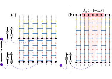
(a)

(b)

Figure 2: Schematic description of the ancilla probes that we use. In both cases, we let the circuit evolve until reaching a stationary state. In (a), we measure a qubit in the system and then arrange it in a Bell state with an ancilla qubit. We then let the system evolve for a time $\tau$, and repeat this process with the same site and a second ancilla. We follow by calculating the mutual information between the two ancillas $\mathcal{I}_{2}(Q_{1},Q_{2})$ over time. In (b), we depict a system with open boundaries. At the initial time we entangle the ancilla $Q$ with the qubit at $x=0$. At later times, we calculate the ancilla’s mutual information with a symmetric segment $A_{x}=[-x,x]$. The information propagation is evaluated using the smallest $x$ for which $\mathcal{I}_{2}(Q,A_{x})>0$.

Specifically, at each instance $t$, we draw the measurement rate across the entire lattice according to the random variable $p(t)=\frac{1}{2}r_{t}^{n}$, where $r_{t}$ are independent random numbers uniformly distributed on $[0,1]$. With this choice, we control the time-averaged measurement rate $\bar{p}$ by varying $n$, with $\bar{p}=1/\quantity(2n+2)$. We note that the limit $n\to 0$ corresponds to a deterministic (time-independent) measurement rate $p(t)=\bar{p}|_{n\to 0}=1/2>p_{c}^{\text{\tiny MIPT}}\approx 0.16$ placing the model in the area-law phase [5, 6, 10]. Whereas, for $n\to\infty$, the measurement rate drops to zero, resulting in unitary dynamics and a volume-law phase. Dynamic rare regions appear from the measurement rate associated with a specific time being greater or lesser than $p_{c}^{\text{\tiny MIPT}}$. We explore the MIPT in this spatially uniform model by varying $n$ and thus $\bar{p}$. Unless stated otherwise, we take periodic boundary conditions.

II.2 Entanglement probes

The main quantities we study are obtained from the bipartite entanglement entropy defined as

$$S(A)=-\text{Tr}_{A}\quantity[\rho_{A}\log_{2}\quantity(\rho_{A})],$$ (2)

with the reduced density matrix $\rho_{A}=\text{Tr}_{A^{C}}\ket{\psi}\bra{\psi}$, for a spatial partition of a segment $A$ and its complement $A^{C}$, and the full system in pure state $|\psi\rangle$. With the above definition, we can construct the bipartite and tripartite mutual information defined as

$$\mathcal{I}_{2}(A,B)\coloneqq S(A)+S(B)-S(A\cup B)$$ (3)

and

$$\mathcal{I}_{3}(A,B,C)\coloneqq\mathcal{I}_{2}(A,B)+\mathcal{I}_{2}(A,C)-\mathcal{I}_{2}(A,B\cup C),$$ (4)

respectively. These latter two quantities can be made particularly useful by choosing appropriate geometries and state preparations with ancillae.

To quantify the scaling of space-time dynamics, we use an ancilla qubit that we entangle with the monitored quantum circuit in two different ways. First, following the protocol of [25, 12] we track the purification time of the ancilla. To do so, we initialize our wave function in a completely scrambled state and then generate a Bell pair between a system qubit and an ancilla qubit. We then let the circuit evolve according to the model described above and measure the bipartite entanglement entropy $S_{Q}$ of the ancilla qubit with the rest of the system. Second, we use the mutual information between two different ancillas. To that end, we first let the system reach a stationary state, then we measure a qubit in the system and put it in a Bell state with an ancilla $Q_{1}$; after $\tau$ timesteps, we repeat this process with a second ancilla $Q_{2}$ and the same qubit. Then we continue running the circuit while calculating the mutual information between the two ancillas at each timestep, $\mathcal{I}_{2}(Q_{1},Q_{2};t)$, see Fig. 2a.

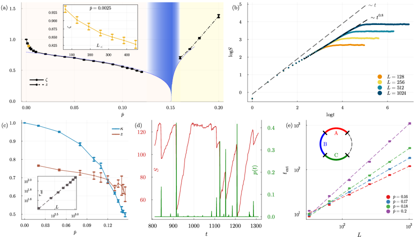
(a)

(b)

(c)

(d)

(e)

Figure 3: (a) The exponent $\zeta(\bar{p})$ (solid black line), controlling the saturated entanglement entropy scaling $S\sim L^{\zeta}$, continuously decreases with an increase in $\bar{p}$ in the entangling phase. Our finite-size numerical estimates suggest $\zeta<1$ even for the smallest positive $\bar{p}$. For $\bar{p}>\bar{p}_{c}$, we depict the dynamical exponent $z$ (dashed black line), evaluated via the entanglement time, $t_{\text{ent}}$, which decreases upon approach to the critical point (b) The temporal evolution of the averaged entanglement entropy with $\bar{p}=0.1$. Different colors denote different system sizes. Within the studied range of system sizes, the pre-saturation growth is sublinear in time. For the presented $\bar{p}$, the exponent $\kappa\approx 0.8$, where $S\sim t^{\kappa}$. (c) The evolution of the exponent $\kappa$ (blue line), which gradually decreases from $\kappa=1$ for a unitary circuit to $\kappa\approx 1/2$ near $\bar{p}_{c}$. Similarly, the dynamical exponent $z$ (red line), defined via the saturation time $\tau_{\text{sat}}\sim L^{z}$, is less than unity throughout the entangling phase. An example for the computation of the exponent $z$ via the saturation time $\tau_{\text{sat}}$ scaling as a function of system size is presented in the inset for $\bar{p}=0.1$. (d) Temporal sawtooth behavior of the half-cut bipartite entanglement entropy for a specific circuit realization. Here $L=256$ and $\bar{p}=0.005$. The green line marks the measurement rate at time $t$, $p(t)$. Each sharp drop in $S$ coincides with a significant peak of $p(t)$ corresponding to a high measurement rate. The sawtooth shape gradually disappears upon approaching criticality. (e) Numerical estimates of the dynamical exponent $z$ in the area-law phase, calculated using finite-size scaling of the entanglement time, defined as the first time for which $\mathcal{I}_{3}(A,B,C)\neq 0$ for any possible partition of the system to $L/4$ segments $\{A,B,C\}$; an example for such a partition is depicted in the inset.

Last, to understand the consequences of this ultrafast dynamics, we monitor the speed at which quantum information spreads, similarly to the scheme presented in [9]. Explicitly, we consider open boundary conditions and let the system evolve for a duration $\tau_{0}$ beyond the saturation time of the average entanglement entropy. Next, we carry out a projective measure on the central qubit and entangle it with a single ancilla qubit to form a Bell pair. We reset our clock to $t=0$ and proceed with the circuit dynamics. At each time instance, as long as the ancilla is still entangled with the system, we calculate the evolution of the bipartite mutual information $\mathcal{I}_{2}(Q,A_{x})$ between the ancilla $Q$ and a symmetric segment of the system around the central qubit $A_{x}\coloneqq[-x,x]$, see Fig. 2b. We denote by $x_{I}(t)$ the smallest $x$ for which $\mathcal{I}_{2}(Q,A_{x})$ is nonvanishing. This quantity serves as a measure of the minimal segment size that allows us to infer information encoded in the ancilla qubit. In the presence of entangling dynamics, for a given segment size $x$ smaller than the full system, information on the ancilla qubit will (provided entanglement with the system remains) typically leak outside the segment, so the mean $x_{I}(t)$ will grow with time and thus give an estimate of the dynamics of information spreading.

Unless specified otherwise, all quantities considered are averaged. Each quantity is averaged over different realizations of the quantum circuit, the initial product state, and the random structure of the measurement rate. Typically, we use at least 3000 different realizations to ensure convergence.

II.3 Infinitely Fast Scaling Ansatz

To guide our exploration, we postulate the anticipated critical space-time scaling of our dynamics by drawing inspiration from the dual problem of quenched, i.e., time-invariant spatial modulations, either random or quasiperiodic [12, 26]. There, the critical dynamics present ultraslow activated scaling of time scales versus the system size $\log t\sim L^{\psi}$, with an activation exponent $\psi$, similarly to the infinite-randomness criticality of random one-dimensional spin chains [27, 28, 29, 30]. This motivates exchanging the roles of space and time, which suggests the following ultrafast critical scaling hypothesis

$$t^{\psi_{\tau}}\sim\log L$$ (5)

for a temporal critical activation exponent $\psi_{\tau}$. In the following, we will test the above scaling ansatz in our model by examining the scaling properties of various observables.

III Results

III.1 Sub-volume law entangling phase

We initiate our analysis by studying the stability of the volume-law phase to the introduction of a time-varying random measurement rate corresponding to a small nonzero $\bar{p}$. To begin, we examine the deviations from the volume-law scaling of the long-time entanglement entropy, $S\sim L$, that is present at $\bar{p}=0$. To that end, we compute the growth exponent associated with the power law ansatz

$$S(L,t\to\infty)\sim L^{\zeta(\bar{p})}~{};$$ (6)

see Fig. 1b. We note that the limit $t\to\infty$ corresponds to times greater than the saturation time of the averaged entanglement entropy. Within the resolution limit of our numerics, we find that the volume-law phase appears to be unstable, with a sudden drop in $\zeta(\bar{p})$ below unity, even for a small $\bar{p}>0$. Further increasing $\bar{p}$ continuously decreases $\zeta$ upon approaching the MIPT. We interpret, and provide direct evidence below, that these results can be understood through a Griffiths effect in time, which leads to a sublinear scaling of the entanglement entropy with system size in the entangling phase, see Fig. 3a. Further increasing $\bar{p}$ beyond the critical value $\bar{p}_{c}$ completely suppresses the growth of the entanglement entropy, leading to an area-law phase.

As additional support, we also examine the bipartite entanglement entropy at late times as a function of the subsystem length $x$ and find a sublinear growth with an exponent $\zeta$, $S(x;L,t\rightarrow\infty)\sim x^{\zeta(\bar{p})}$ (for $x\ll L$) that agrees well with the previous analysis. As before, ${\zeta(\bar{p})}$ continuously decreases with increasing $\bar{p}$, see Appendix A. This sublinear growth of the late-time entanglement with $x$ is the space-time rotation of the sublinear in time growth of entanglement in the model with quenched randomness [12], so is thus as expected.

We now turn to study the real-time dynamics of the half-cut entanglement entropy. Again, we allow for a power-law scaling deviating from linearity at times $t\ll L$,

$$S(t,L)\sim t^{\kappa}.$$ (7)

To extract the temporal exponent $\kappa$, we examine the growth of the averaged $S$ at early times, prior to saturation, see for example Fig. 3b. Importantly, curves of different system sizes share the same trajectory before smaller systems reach saturation, and this shared window represents the thermodynamic value and is used to calculate $\kappa$. Within the entangling phase, $\kappa$ gradually decreases from $\kappa=1$ at the unitary point to $\kappa\approx 1/2$ near criticality, as shown in Fig. 3c. Further analysis of the pre-saturation dynamics via the lens of the clipped gauge stabilizer length statistics is given in Appendix B.

The unconventional spatial and temporal power-law scaling exponents, in the above respective limits, suggest a nontrivial dynamical exponent, $z$, relating space and time length scales. To compute $z$, for a given system size $L$, we estimate the saturation time $\tau_{\text{sat}}(L)$, defined as the time at which the entanglement entropy in the thermodynamic limit reaches its saturation value, $S_{\text{sat}}(L,t\to\infty)$, for a given finite system size $L$, see Appendix C. We then extract $z$ from a power-law fit to the scaling form $\tau_{\text{sat}}(L)\sim L^{z}$, see the inset of Fig. 3c.

Interestingly, the dynamical exponent $z$, is directly related to the exponents pair $\kappa$ and $\zeta$. From the above discussion, it follows that $S_{\text{sat}}(L)\sim\tau_{\text{sat}}^{\kappa}(L)\sim L^{\zeta}$, such that $\tau_{\text{sat}}\sim L^{\zeta/\kappa}$. Consequently, we identify

$$z=\zeta/\kappa.$$ (8)

We numerically verify this relation explicitly in Appendix C. A key observation is that in the sub-volume-law phase, $\zeta(\bar{p})<\kappa(\bar{p})\leq 1$ for all $\bar{p}$, which, when combined with Eq. 8, implies that $z$ is less than unity across the entire phase, as depicted in Fig. 3c. This allows us to conclude that dynamics, throughout the entangling phase, is dominated by Griffiths effect.

The evident sub-linear growth of the long-time entanglement with $L$ is surprising, but a natural consequence of temporal rare region effects. To illustrate the origin of this phenomenon, we present in Fig. 3d a typical time trace of the entanglement entropy for a specific random circuit realization, characterized by a relatively small average measurement rate ($\bar{p}=0.005$). With the above choice, for the most part $p(t)$ is extremely small, interleaved by rare time instances that have a high measurement rate. The resulting temporal evolution follows a “sawtooth” structure, with intermittent volume-law like behavior, by which the entanglement grows linearly following a sudden drop due to a series of measurements. Specifically, $p(t)$ instances of high measurement rates give rise to an abrupt drop in the entanglement entropy, followed by a recovery period, during which $S$ grows linearly with time, attempting to exhaust its maximum value $L/2$. We emphasize that the maximal value of $S$ is $L$-dependent, whereas the rate of occurrence of large $p(t)$ events is $L$-independent. The competition between the above two mechanisms is at the core of the nontrivial $L$-dependency of the average entanglement entropy. For small $\bar{p}$ values, this behavior and the sublinear growth are captured by an effective heuristic model, presented in Appendix D.

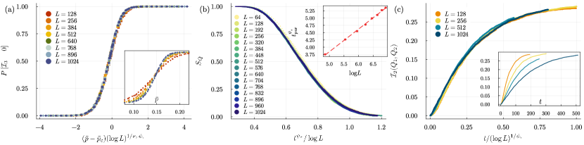
(a)

(b)

(c)

Figure 4: (a) Curve collapse analysis of $P\quantity[\mathcal{I}_{3}=0]$, according to the ansatz in Eq. 10, yields an horizontal axis scaling with the values $\bar{p}=0.151$ and $\nu_{\tau}\psi_{\tau}=0.6$. The unscaled data is depicted in the inset. (b) The ancilla survival rate $S_{Q}$ and (c) the mutual information between two ancillas separated by $\tau=16$ scale as $t^{\psi_{\tau}}\sim\log L$ with $\psi_{\tau}=0.3$. The inset in (b) shows that the same scaling applies to the average ancilla purification time, namely the average time it takes an ancilla to disentangle from the system completely.

III.2 Area law phase

Generally, a high measurement rate contributes to teleportation and allows the information to spread super-ballistically, breaking the Lieb-Robinson bound [31, 9]. However, many measurements also suppress the entanglement and may restrict its spreading. We hypothesize that the critical point is exactly where the interplay between teleportation and entanglement suppression leads to the fastest growth of the entanglement range. Therefore, we expect the dynamical exponent $z$ to be smallest at $\bar{p}_{c}$ and grow again upon increasing the measurement rate.

To study the behavior of the dynamical exponent in the area-law phase, we look for the first time in which long-range entanglement emerges. Concretely, we initialize the system in a random product state and monitor the growth of entanglement by tracking the tripartite mutual information, $\mathcal{I}_{3}(A,B,C)$, across all possible partitions $\{A,B,C\}$ of the system, where $A,B,C$ are adjacent quarters. We identify the first time when $\mathcal{I}_{3}(A,B,C)\neq 0$, serving as a typical time for the emergence of long-range entanglement, and examine how this time scales with the system size $L$, positing an $t_{\text{ent}}\sim L^{z}$ scaling relation. We note that this time is associated with rare events that become increasingly rare with the increase in $\bar{p}$.

Indeed, as we show in Fig. 3e, the exponent $z$ grows in the area-law phase. Overall, completing the picture of minimal, vanishing $z$ at $\bar{p}_{c}$ and a temporal Griffith fan opening from both sides, as presented in Fig. 3a.

III.3 Infinitely fast fixed point

Motivated by the above findings, we now turn to study the phase transition separating the sub-volume- and area-law phases. To determine the critical properties, we postulate the emergence of a diverging time scale (i.e. a correlation time) close to criticality, with a power-law scaling

$$\tau\sim|\bar{p}-\bar{p}_{c}|^{-\nu_{\tau}},$$ (9)

for a correlation time exponent $\nu_{\tau}$. We choose to work with this definition as it is much more natural. This is rather clear when we write the problem in terms of a correlation length $\xi\sim|\bar{p}-\bar{p}_{c}|^{-\nu}$ and $\tau_{\xi}\sim\xi^{z}\sim|\bar{p}-\bar{p}_{c}|^{-\nu z}$. The implied relation based on the above is $\nu_{\tau}=\nu z$, however we expect ultrafast dynamics, i.e., $z\rightarrow 0$ and hence $\nu\rightarrow\infty$ such that $\nu_{\tau}$ is a constant (as we show below).

Due to temporal rare regions, the distribution of $P[\mathcal{I}_{3}]$ is broad, see Appendix E, and a similar approach to the infinite-randomness transition can be employed based on $P\quantity[\mathcal{I}_{3}=0]$: In the sub-volume law phase we will always find an entangled region of the system, while on the area law side the probability that a region is disconnected becomes unity. Combining the above scaling relation with Eq. 5, we obtain a generalized finite-size scaling ansatz for the universal amplitude $P\quantity[\mathcal{I}_{3}=0]$ [10, 32, 12]

$$P\quantity[\mathcal{I}_{3}=0](\bar{p},L)\sim f\quantity[\quantity(\bar{p}-\bar{p}_{c})\quantity(\log L)^{1/\quantity(\nu_{\tau}\psi_{\tau})}],$$ (10)

Here, $f(x)$ is a universal scaling function.

We employ the standard finite size scaling curve collapse analysis according to Eq. 10 to provide a numerical estimate of the critical average measurement rate $\bar{p}_{c}=0.150(3)$ and the product of critical exponents $\nu_{\tau}\psi_{\tau}=0.58(2)$, see Fig. 4a and additional analysis in Appendix F. Crucially, the critical properties do not follow the scaling relation associated with the unperturbed MIPT [6, 5, 10]. In particular, attempting a power-law (instead of activated) spacetime scaling fails to produce an accurate curve collapse and results in the anticipated running exponents with systems size, see Appendix F.

As a complementary analysis, allowing us to extract $\psi_{\tau}$ directly (without the multiplicative factor $\nu_{\tau}$), we study the critical dynamics of an ancilla qubit at criticality $\bar{p}=\bar{p}_{c}$. We employ the space-time scaling ansatz Eq. 5 on the time evolution of $S_{Q}$ for varying system sizes by presenting the temporal axis in terms of the scaling variable $t^{\psi_{\tau}}/\log L$, see Fig. 4b. We obtain a curve collapse for $\psi_{\tau}=0.30(2)$. Our error estimate includes the uncertainty in computing $\bar{p}_{c}$. Combining the above two results for the critical exponents, we can numerically estimate the correlation time exponent, defined in Eq. (9), to be $\nu_{\tau}\approx 1.9(2)$, thus saturating (a space-time rotated) Harris bound within the error bars as was seen for the rotated model in [12, 26]. A similar estimate for $\psi_{\tau}=0.30(2)$ was obtained using the purification time, defined as the time at which the ancilla qubit disentangles from the system, as shown in the inset of Fig. 4b. This key finding provides direct evidence for the ultra-fast dynamical scaling of Eq. 5. We further corroborate this result using the mutual information between two ancillas separated by time $\tau=16$, as described in Fig. 2a, and in Fig. 4c we show that, indeed, the data scales well for different system sizes.

Employed with this definition of the temporal critical exponents, we find our results are consistent with a dynamical Harris criterion. Namely that the infinitely fast fixed point flows to a value that saturates the Harris bound for disordered systems, with its suitable spacetime rotation, leads us to the general dynamical hypothesis $\nu_{\tau}\geq 2$, Eq. 1 which our results saturate.

In that regard, Ref. [33] proposed a complementary bound, $z\nu\geq 2$, relating the dynamical exponent $z$ and the spatial correlation length $\nu$. This entails a divergence of the correlation length exponent, $\nu\to\infty$, upon approaching our critical point with $z\to 0$ and $\nu_{\tau}=\nu z=1.9(2)$ goes to a finite value saturating the bound.

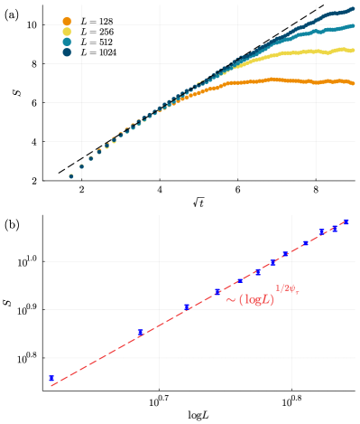
(a)

(b)

Figure 5: (a) The saturated entanglement entropy grows at the critical point as $S\sim t^{1/2}$, a direct rotation of the infinite-randomness model. (b) Combined with the ultrafast scaling, we derive the system size dependence of the saturated entanglement entropy $S\sim\quantity(\log L)^{1/2\psi_{\tau}}$, with $\psi_{\tau}=0.32(3)$

.

It is interesting to understand the universal growth of the entanglement entropy at criticality. We begin by drawing inspiration from the spacetime-rotated infinite-randomness problem [12], for which $S(L,t\rightarrow\infty)\sim L^{1/2}$ and $S(L\rightarrow\infty,t)\sim\log t$. By combining this perspective with the spacetime scaling of Eq. 5, we postulate that critical entanglement evolution should follow an ultrafast scaling form

$$S(L\rightarrow\infty,t)\sim\sqrt{t},$$ (11)

$$S(L,t\rightarrow\infty)\sim(\log L)^{\frac{1}{2\psi_{\tau}}}$$ (12)

We find both of these forms to be consistent with our numerical results, as shown in Fig. 5b. We caution that a precise numerical estimate of the temporal growth exponent is challenging to extract due to our limited time window before saturation in our finite-size simulations. On the other hand, for the finite size scaling, we find excellent agreement with the above scaling form.

A generalized Widom scaling curve collapse analysis is given in Appendix F. It is useful to contrast this evolution with the logarithmic growth in space and time in the Lorentz invariant MIPT.

III.4 Information Propagation

Given all of the evidence of the infinitely fast fixed point, we now turn to implications for quantum information propagation. We study the pace of the information propagation in $x_{I}(t)$, as defined above, see also Fig. 2b. In Fig. 6a, we depict $x_{I}(t)/L$ for a range of systems sizes, at criticality. Plotting the temporal axis with the scaling variable $t/(\log L)^{1/\psi_{\tau}}$ using the previously calculated $\psi_{\tau}=0.3$, leads to a curve collapse, as before, which nontrivially supports our ultrafast scaling ansatz.

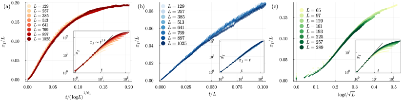
(a)

(b)

(c)

Figure 6: (a) At the critical point of the temporally disordered model, the information distance, divided by the linear system size, $x_{I}/L$, follows the ultrafast ansatz (Eq. 5), with $\psi_{\tau}=0.3$. The inset suggests a super-ballistic propagation $x_{I}\sim t^{\alpha}$ with $\alpha\approx 1.4$. (b) The information distance evaluated for the uniform MIPT displays a conformal symmetry as seen via the linear space-time scaling, $t/L$. The information spreads linearly with time with a velocity of $v=1$, as shown in the inset. (c) At the infinite-randomness fixed point, the information distance follows an ultraslow activated dynamics $x_{I}/L=f\quantity(\log t/\sqrt{L})$ and overall sublinear time evolution (see inset).

Moreover, we explore the early time dynamics of information spreading at criticality, as shown in the inset of Fig. 6a. We observe a super-ballistic growth, where $x_{I}(t)\sim t^{\alpha}$ with $\alpha\approx 1.4$. This result should be contrasted with the relativistic dynamics of the uniform MIPT, for which $x_{I}^{\text{MIPT}}(t)=t$ as directly presented in Fig. 6b.

To complete the picture and classify the rate of information propagation in the three classes of fixed points we have considered in this work (that have $z\rightarrow 0$, $z=1$, and $z\rightarrow\infty$), we compute $x_{I}$ also at the infinite-randomness criticality (in the model in Ref. [12]). There, the activated scaling, takes place with $x_{I}/L$ being a function of the scaled space-time variable $\log t/\sqrt{L}$, see Fig. 6c. This ultraslow dynamic also leaves its mark on our computational efforts and limits us to relatively small system sizes, which makes the determination of the power, or perhaps logarithm, with which $x_{I}$ grows especially challenging with time. Still, in the inset of Fig. 6c, we show that, at the infinite-randomness fixed point, the information spreads slower than linear. Overall, introducing randomness to the system allows us to travel from a very slow information propagation point to a super-ballistic fixed point beyond the Lieb-Robinson bound.

Lastly, we note that $x_{I}$ allows us to directly observe teleportation events, through jumps at instants in time that take place in individual samples and are at the core of the superluminal behavior we have uncovered. In Appendix G, we demonstrate this effect in a specific circuit realization where teleportation manifests in an abrupt jump in $x_{I}$.

IV Discussion

In this work, we have examined hybrid circuit dynamics that follow an inherently non-stationary protocol, realized via a time-dependent and random average measurement rate. The associated circuit dynamics present a competition between time instances that experience few measurements and thus entanglement production vs. other times with many measurements and thus entanglement suppression.

Notably, the resulting emergent phenomena give rise to an unusual entangling phase characterized by a sub-volume growth of the entanglement entropy. We understand this behavior as a Griffiths-like effect dominated by strong measurement events that suppress the entanglement entropy even for weak $\bar{p}$. We further show that the transition from this novel phase to the area-law phase displays nontrivial scaling relations that qualitatively match the spacetime-rotated infinite-randomness picture. A striking feature is that this criticality is characterized by ultrafast dynamics with a vanishing dynamical exponent $z\to 0$. This basic building block allows us to numerically estimate the relevant universal properties, including scaling functions and critical exponents associated with the entanglement entropy growth, temporal fluctuations, and information spreading.

One of our findings is that the entanglement entropy appears to grow sublinearly in time, prior to saturation, in the entangling phase. In this regime, we do not anticipate that boundary conditions would affect the dynamics, and hence, predictions based on space-time rotation are expected to hold. In particular, in the quenched disorder model, a volume-law phase $S\sim L$ was expected at low measurement rate, but not carefully tested [12] and, preliminary results (not shown) suggest sub-volume-law behavior instead, a detailed study of which we leave for future work. $S\sim L$ would translate under space-time rotation to linear-in-time growth of the entanglement entropy in the temporally disordered model. However, our numerical estimates suggest a sublinear-in-time growth. This discrepancy can result from a slow, finite-size flow of exponents beyond the reach of our numerical calculations. A more interesting possibility would be if this is indicating true asymptotic deviation from volume-law entanglement scaling in the quenched disorder model and from linear-in-time entanglement growth in the temporally-disordered model, thus telling us that these entangling phases are in this sense critical. We leave this open question to future studies.

Our results show that the correlation time critical exponent $\nu_{\tau}\cong 2.0$, suggesting a temporal CCFS bound whose limit is saturated by this model.

Looking to the future, it would be interesting to further engineer the properties of the dynamics by varying the properties of the temporal modulations, e.g. by considering hyperuniform distributions or quasiperiodic modulations. This can potentially allow us to control the activation exponent $\psi_{\tau}$ and associated critical exponents [26]. Of specific importance would be employing the infinitely fast properties uncovered in this model in the engineering of efficient quantum algorithms and state preparation on quantum computers through the use of feedback based on the measurement outcomes.

Appendix A Entanglement entropy scaling with partition segment size

As shown in the main text, in the entangling phase, the finite size scaling of half-cut bipartite entanglement entropy displays a sublinear scaling, deviating from the standard linear growth. Here, we further support this observation via a complementary analysis by tracking the evolution of the entanglement entropy as a function of the partition segment length $x$. In a standard volume-law phase, $S(x)$ is anticipated to grow linearly with $x$ (up to logarithmic corrections) [5]. By contrast, in agreement with our previous results, for temporally random models, we find a sublinear scaling $S(x)\sim x^{\zeta(\bar{p})}$, as shown Fig. 7. Crucially, the numerical estimates of $\zeta(\bar{p})$ match the finite size scaling of the half-cut entropy Fig. 1b.

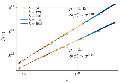
Figure 7: The entanglement entropy versus the partition length $x$, in the entangling phase, for a fixed $\bar{p}=0.05,0.1$. Different curves correspond to different system sizes. Dashed lines are a fit to a power law form.

Appendix B Pre-saturation dynamics of stabilizers length statistics

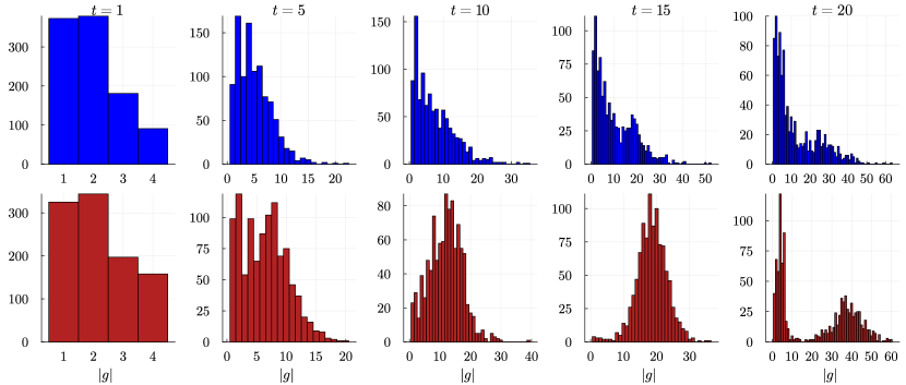
Figure 8: Evolution of stabilizer length distributions $|g|$ at selected time steps. Upper panels (blue) show the progression for a circuit with uniform measurement rate $p=0.1$, while lower panels (red) demonstrate the dynamics under temporally random measurements with an average rate $\bar{p}=0.1$.

In this section, we examine the temporal evolution of the stabilizer length statistics within the clipped gauge framework [6, 5]. To that end, we simulate a sufficiently large system size comprising $L=1024$ qubits, allowing us to study the dynamics for broad pre-saturation time windows. Results are presented for open boundary conditions. We consider both uniform and temporally random measurement rates. Our focus is on the early stages of circuit evolution, for which hybrid circuit dynamics exhibit a linear-in-time entanglement entropy growth for the uniform case. Whereas the temporally random model, as shown in the main text, demonstrates a sublinear growth $S(t)\sim t^{\kappa}$, with an exponent $\kappa\leq 1$ that varies with $\bar{p}$.

In the clipped gauge, the entanglement entropy of a segment $A$ is defined by [9]

$$S(A)=|A|-|\{g\in\mathcal{S}\,|\,\text{supp}(g)\subseteq A\}|,$$ (13)

where $\mathcal{S}$ is a set of generators of the stabilizers group in the clipped gauge, and $\text{supp}(g)$ is the spatial support of the generator $g$ as defined by the clipped gauge conditions. With the above definition in mind, we can correlate the generator statistics and the entanglement entropy by noting that short stabilizers correspond to short-range entanglement (low entanglement entropy), whereas long stabilizers indicate long-range entanglement (high entanglement entropy).

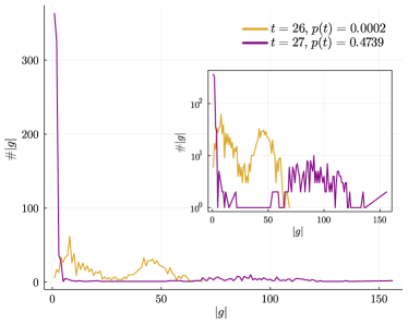
Figure 9: Impact of a strong measurement event ($p(t)=0.4739$) on stabilizer length distribution. The comparison of distributions immediately before and after the event illustrates that while most stabilizers are shortened, the remaining ones are enlarged due to teleportation.

Fig. 8 tracks the temporal evolution of the distribution of stabilizer lengths in a single circuit realization. We compare a uniform measurement rate (upper panels, blue) and temporally random measurement rate (lower panels, red), both with $\bar{p}=0.1<\bar{p}_{c}$. We observe that the standard uniform model develops a concentration of short stabilizers associated with measurement events and a gradually increasing tail of long stabilizers generated primarily by unitary dynamics. By contrast, the temporally random model alternates between qualitatively distinct forms: 1) Time periods characterized by weak $p(t)$ (nearly unitary evolution) for which the distribution is concentrated at a finite typical stabilizer size with a growing in time mean value. 2) Post-strong measurement events, which dramatically shorten most stabilizers while simultaneously enlarging a fraction of stabilizers via teleportation. A concrete example of the latter is demonstrated in Fig. 9.

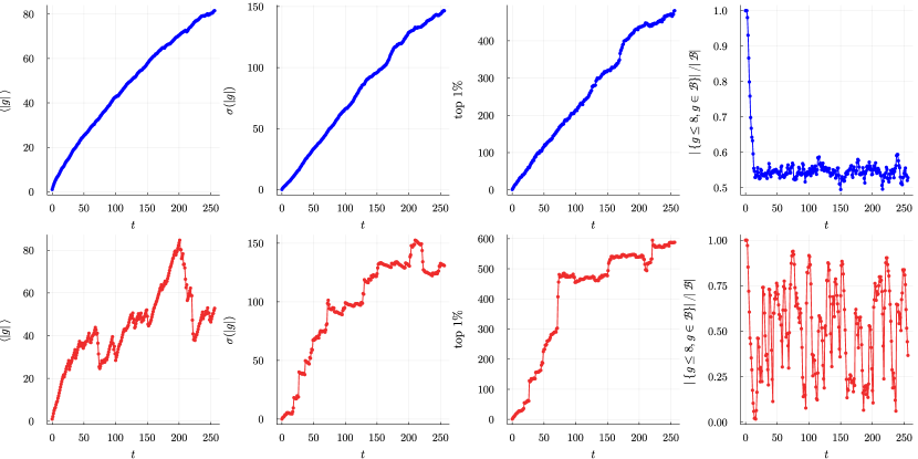
Figure 10: Temporal evolution of key statistical metrics for uniform measurement rate (upper row) and temporally random measurements (lower row), both with $\bar{p}=0.1$. From left to right – first panel: mean stabilizer length; second panel: distribution standard deviation; third panel: the length of the stabilizer at the top 1%; fourth panel: fraction of short stabilizers (length $\leq 8$ qubits). These metrics highlight the contrasting dynamics between uniform and random measurement protocols.

The above evolution patterns are also revealed by examining several statistical metrics of the stabilizer length distribution, such as the mean, standard deviation, and the proportion of short stabilizers, as analyzed in Fig. 10. The uniform $p$ model exhibits smooth, monotonic growth in both the mean length and the standard deviation ($\sigma(|g|)\sim t$), with rapid convergence in the fraction of short stabilizers. The temporally random model, however, demonstrates notably different behavior, characterized by irregular, non-monotonic evolution in all these metrics driven by rare strong measurement events.

Appendix C Computation of the dynamical exponent $z$

To pin down the dynamical exponent $z$ in the entangling phase, we study the finite size scaling of typical time scales associated with the evolution of the entanglement entropy.

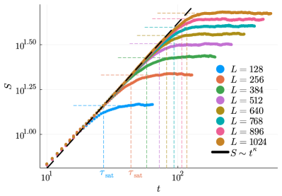
Figure 11: The temporal evolution of the entanglement entropy for $\bar{p}=0.1$. To evaluate the saturation time, we first ensure convergence to the thermodynamics limit, which follows a power-law scaling form $S\sim t^{\kappa}$, with $\kappa=0.81(2)$ . Then, we project the saturation value of the entanglement entropy at a given system size $L$ to the infinite system size curve. The intersection point sets the saturation time $\tau_{\text{sat}}(L)$.

We primarily focus on the entanglement entropy saturation time. This is achieved by initializing a random product state and tracking the evolution of the entanglement entropy for varying system sizes. As explained in the main text, in the thermodynamic limit $L\to\infty$, the entanglement entropy follows a power-law growth as $S\sim t^{\kappa}$. This is exemplified in Fig. 11, where the pre-saturation evolution of curves corresponding to an increasing range of system sizes converges to the thermodynamic limit. The saturation time is then defined as the time at which the entanglement entropy in the thermodynamic limit reaches its saturation value of a given finite size system. This analysis is summarized in Fig. 11. The dynamical exponent $z$, is then evaluated by a a fit to the standard space-time scaling form. $\tau_{\text{sat}}\sim L^{z}$ [12].

To support the above calculation, we also compute typical time scales via two additional approaches. The first observable is the relaxation time extracted from the temporal autocorrelation function of the entanglement entropy, evaluated at late times, beyond the averaged saturation time. Explicitly $R_{S}(\tau)=\langle S(t)S(t+\tau)\rangle_{t\gg\tau_{\text{sat}}}-\langle S(t)\rangle^{2}$. Assuming an exponential decay, we extract the corresponding decay factor $T$ for a given system size $L$ [34]. The second is the entanglement time $t_{\text{ent}}$ associated with the tripartite mutual information defined in the main text.

The above analysis is summarized in Fig. 12a. Importantly, all methods yield approximately the same $z(\bar{p})$. In particular, as mentioned in the main text, the dynamical exponent is well below unity throughout the entangling phase. Lastly, in Fig. 12b, we test the exponent relation Eq. 8, by comparing the exponent product $\kappa z$ to $\zeta$ and find excellent agreement.

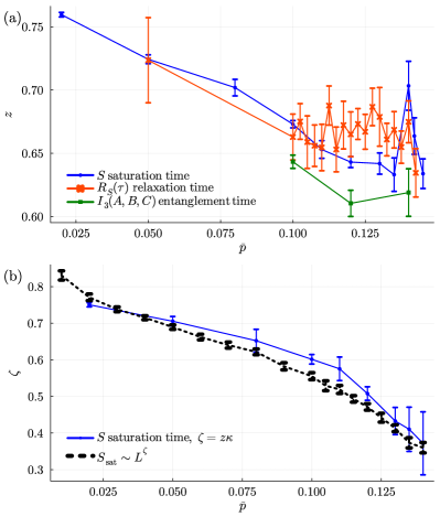
(a)

(b)

Figure 12: (a) the dynamical exponent $z$ as was calculated using the entanglement entropy growth (in blue), the autocorrelation relaxation time (in red) and the entanglement time (in green). (b) The values of $\zeta$ from Fig. 3a against the product of $z$ and $\kappa$ calculated from the space and time scaling of $S$ (in blue).

Appendix D Dynamics of the entanglement entropy in the entangling phase

Figure 13: The temporal randomness probability distribution function, $p(t)$, with $\bar{p}=0.1$ and $\bar{p}=\bar{p}_{c}=0.15$. Most events are with a vanishingly small $p$, but a long tail of high $p$ values appears.

In this section, we analyze the dynamical properties of the entanglement entropy in the entangling phase. By design, the temporal distribution is constructed such that for small $\bar{p}$, most outcomes of $p(t)$ are significantly smaller than the critical measurement rate $p_{c}^{\text{\tiny MIPT}}$ belonging to the uniform MIPT model. Nevertheless, it still allows rare events with $p(t)$ values corresponding to strong measurement rates. For instance, the probability distribution function $p(t)$ with $\bar{p}=0.1$ and $\bar{p}=\bar{p}_{c}=0.15$ is shown Fig. 13.

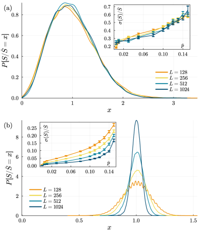
Figure 14: The distribution of the entanglement entropy divided by its mean value, $S/\bar{S}$ for $\bar{p}=0.1$ in the (a) temporally random model and (b) the uniform model. In the temporally random model, the distribution is invariant with system size. This implies that the standard deviation of $S$ scales as the average value $\bar{S}$, which is also shown in the inset. In the uniform model, the distribution converges to a deterministic function, meaning that the standard deviation of $S$ scales slower with $L$ compared to the average value. The inset of (b) suggests that the fluctuations (scaled by system size) around the mean value will vanish in the thermodynamic limit. For visibility considerations, we used kernel density estimation in plotting the distributions.

From the above discussion, we can identify two distinct dynamical regimes: i) In the absence (or weak rate) of measurements, the entanglement entropy is expected to grow linearly with time, bounded from above by half the system size. ii) Following the rare instance of strong measurements, we expect a sharp drop in the entanglement entropy. Combining the above two behaviors leads to the aforementioned sawtooth structure shown in Fig. 3d. Given the above reasoning, one would expect a broad distribution of $S(t)$ resulting from the abrupt drop in values following strong measurements and the slow climb toward saturation during weak measurement periods, seen in Fig. 14 and contrasted with the standard volume law phase. An interesting figure of merit for the broad distribution is the ratio between the standard deviation and the mean. While the standard volume law phase $\sigma(S)/\bar{S}$ tends to zero in the thermodynamic limit, for temporal randomness, they are of the same scale, see Fig. 14.

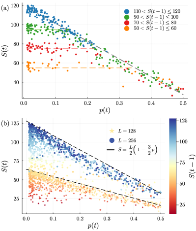
(a)

(b)

Figure 15: (a) Scatter plot of $S(t)$ following an instance of measurement rate $p(t)$ for $L=256$. Different colors represent different ranges of $S(t-1)$. For sufficiently large $p(t)$, the spread of $S(t)$ weakly depends on $S(t-1)$. The dashed lines are guides to the eye and agree with the definition of $Q(L,p(t),S(t-1))$ described in the text. (b) The entanglement entropy immediately after a measurement $p(t)$. The color of the marker indicates the entanglement entropy value before this measurement. All data points were measured for $\bar{p}=0.005$.

In the following, we construct a simple heuristic stochastic dynamical model that attempts to capture the sawtooth structure and the sublinear scaling. Explicitly, we suggest the following dynamics:

$$S(t)=\begin{cases}\min(L/2,S(t-1)+1)&p(t)<p_{0}\\ Q(L,p(t),S(t-1))&p(t)>p_{0}\end{cases}$$ (14)

In the above equation, $p(t)$ is the measurement rate at time $t$, as defined above. The first line corresponds to the linear rise of entanglement entropy for a weak measurement rate, bounded from above by the saturation value. $p_{0}$ serves as an upper cutoff for the weak measurement regime. The second line corresponds to strong measurement events, followed by a shape decrease of the entanglement entropy as captured by the random function $Q(L,p(t),S(t))$, which we estimate empirically below.

In Fig. 15a, we use a scatter plot to assess the values of $S(t)=Q(L,p(t),S(t-1))$, given $S(t-1)$ and $p(t)$ for $L=256$. We note that $Q(L,p(t),S(t-1))$ depends on $S(t)$ only as an upper bound. In particular, $S(t)$ for sufficiently large $p(t)$ is dominated by the values of $p(t)$ and displays a weak dependence on $S(t-1)$, as long as $S(t-1)>S(t)$.

To quantify this observation, we construct an effective data-based model, where we estimate the statistics of $S(t)$ values resulting from a single circuit layer with a specific $p(t)$ given $S(t-1)$ and the system size $L$. In Fig. 15b, we show that measuring at a measurement rate of $p$ results in an upper bound on the entanglement entropy immediately after this time instance to $g_{\text{\tiny upper}}(p,L)\coloneqq\max S\quantity(t|p\quantity(t)=p)=\frac{L}{2}\quantity(1-\frac{3}{2}p)$. The average value of $S$ follows a similar relation $g_{\text{\tiny av}}(p,L)\coloneqq\left\langle S\quantity(t|p\quantity(t)=p)\right\rangle=\frac{4L}{9}\quantity(1-\frac{3}{2}p)$. We utilize those results to construct a probability distribution function for $Q(L,p(t),S(t-1))=\min\quantity(q,S(t-1))$. Our first choice for $P[q]\sim q^{\gamma}$ such that $q_{\max}=g_{\text{\tiny upper}}\quantity(p\quantity(t),L)$ and $\langle q\rangle=g_{\text{\tiny av}}\quantity(p\quantity(t),L)$, explicitly, $\gamma=\quantity[g_{\text{\tiny upper}}\quantity(p\quantity(t),L)/g_{\text{\tiny av}}\quantity(p\quantity(t),L)]-1$. As a second choice, we take $P[q]$ to be normally distributed, with a mean $g_{\text{\tiny av}}(p,L)$ and standard deviation $g_{\text{\tiny std}}(p,L)=\frac{\sqrt{L}}{4}$ to match the data.

We simulated Eq. 14, with $\bar{p}=0.005$, and analyzed resulting stochastic dynamics. We found that with either choice of distributions, we successfully capture the sublinear growth of the entanglement entropy $S\sim L^{\zeta}$ with $\zeta\approx 0.8$ with power-law distribution and $\zeta\approx 0.75$ with normal distribution, see Fig. 16

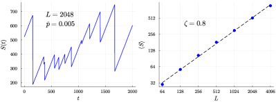
Figure 16: (Left) Sawtooth dynamics of $S(t)$ as generated by the toy model Eq. 14 (Right) $L$ scaling of the average $S_{t}$ at long times, for $\bar{p}=0.005$, and power-law in distribution $p[q]$ in Eq. 14, which yields $\zeta=0.8$, in agreement with the Clifford circuit simulation.

We emphasize that our effective model qualitatively captures the dynamics of the full circuit dynamics only in the limit of small $\bar{p}$.

Appendix E Statistics of $\mathcal{I}_{3}$

In the main text, we employed the observable $P\quantity[\mathcal{I}_{3}=0]$ to detect the critical point and extract critical exponents. This choice allows taming strong finite size effects associated with temporal rare regions that lead to a broad $\mathcal{I}_{3}$ distribution. In Fig. 17, we depict histograms of $\mathcal{I}_{3}$ in various regimes, which indeed displays a broad distribution, motivating the focus on the finite-size analysis of $P\quantity[\mathcal{I}_{3}=0]$. The different tendencies of $P\quantity[\mathcal{I}_{3}=0]$ between the two phases and the plateau near criticality are manifest in the scaling across a wide region of $\bar{p}$ values, which we used in Fig. 4a.

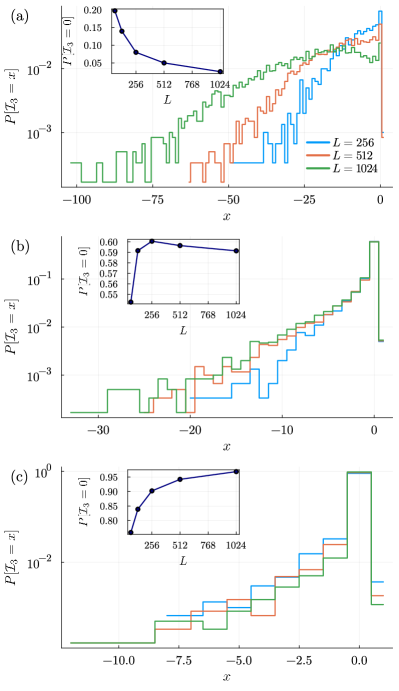
Figure 17: Histograms of $\mathcal{I}_{3}$ at $\bar{p}=0.1$, in the sub-volume-law phase (a), $\bar{p}\approx\bar{p}_{c}=0.15$ (b) and at $\bar{p}=0.18$ in the area-law phase (c). The insets finite scaling of $P\quantity[\mathcal{I}_{3}=0]$ in the different phases.

Appendix F Detailed analysis of critical data extraction via finite-size scaling

This section offers a detailed analysis of the numerical methods employed to determine the critical point and related universal critical exponents. An accurate method for extracting the critical point and critical exponents is considering pairs of system sizes $L_{<}$ and $2L_{<}$. For each pair, we find the intersection of $P\quantity[\mathcal{I}_{3}=0]$ curves, which set the finite size value of the critical point $\bar{p}_{c}\quantity(L_{<})$. In addition, the derivate

$$g(L_{<})=\frac{dP\quantity[\mathcal{I}_{3}=0](\bar{p},L)}{d\bar{p}}|_{\bar{p}_{c}\quantity(L_{<})}$$ (15)

with respect to a deviation from criticality is anticipated to follow the scaling $g(L)=\quantity(\log L)^{1/(\nu_{\tau}\psi_{\tau})}f^{\prime}(0)$, according to our ansatz in Eq. 10. In Fig. 18, we summarize the above analysis. We indeed find a convergence to the critical measurement rate $p_{c}=0.150(3)$ as a function of system size and an excellent agreement with the scaling ansatz, allowing for an accurate estimation of exponents product $\nu_{\tau}\psi_{\tau}$.

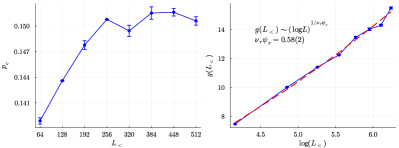
Figure 18: (Left) The critical point as evaluated using the intersection of pairs of $P\quantity[\mathcal{I}_{3}=0]$ curves. The $\bar{p}_{c}$ value converges to $\bar{p}=0.150(3)$. (Right) The derivative of $P\quantity[\mathcal{I}_{3}=0]$ at the critical point grows as $\quantity(\log L)^{1/(\nu_{\tau}\psi_{\tau})}$ with $\nu_{\tau}\psi_{\tau}=0.58(2)$.

Next, we compute the entanglement entropy scaling function at long times, extending the critical scaling form $S(\bar{p}_{c})\sim\quantity(\log L)^{1/2\psi_{\tau}}$, as verified in Fig. 5b. For small deviations from criticality, we expect the generalized scaling form to hold,

$$S(p,L)=\quantity(\log L)^{1/2\psi_{\tau}}f\quantity[\quantity(\bar{p}-\bar{p}_{c})\quantity(\log L)^{1/(\nu_{\tau}\psi_{\tau})}].$$ (16)

Utilizing the previously calculated values $\psi_{\tau}\approx 0.3$ and $\nu_{\tau}\psi_{\tau}\approx 0.6$, without further tuning parameters, indeed yields a Widom scaling curve collapse, presented in Fig. 19.

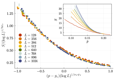
Figure 19: Widom scaling of the bipartite entanglement entropy with the pre-calculated values of $\psi_{\tau}$ and $\nu_{\tau}\psi_{\tau}$. The inset shows the data before scaling.

Lastly, to rule out a power-law space-time scaling relations at criticality, we attempt to fit $P\quantity[\mathcal{I}_{3}=0]$ to the standard power-law ansatz $P\quantity[\mathcal{I}_{3}=0]\sim f\quantity[\quantity(\bar{p}-\bar{p}_{c})L^{1/\nu}]$ for a sequence of increasing system sizes ranges, starting with $L_{<}$. We find a running in system size exponent, suggesting an RG flow to a vanishing exponent consistent with activated logarithmic scaling as our ultrafast ansatz.

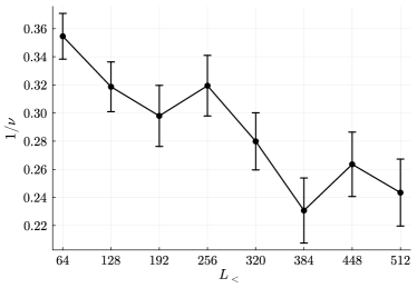
Figure 20: The correlation length critical exponent as extracted from the standard ansatz $P\quantity[\mathcal{I}_{3}=0]\sim f\quantity[\quantity(\bar{p}-\bar{p}_{c})L^{1/\nu}]$ decreases with the increasing system size.

Appendix G Teleportation events in the information propagation

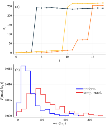
(a)

(b)

Figure 21: (a) Measurement-induced teleportation demonstrated through the information propagation $x_{I}$ in specific circuit realizations with $L=1025,\,\bar{p}=0.05$. Each color represent a different sample. (b) The probability distribution of the maximum single-step increase in $x_{I}$ for uniform (blue) and temporally random (red) measurement patterns at their critical point $p_{c}^{\text{\tiny uni}}\cong 0.16$ and $p_{c}^{\text{\tiny rand}}\cong 0.15$. Importantly, we only consider samples in which the ancilla survived longer than 32 time steps.

As discussed in the main text, measurements can induce teleportation, which expands the range of entanglement. In the context of the information propagation metric $x_{I}$, such teleportation events would immediately increase the distance the information travels. The essence of teleportation is manifested in the averaged $x_{I}$ quantity by the superluminal dynamics, which could not have occurred by merely unitary dynamics that only allows an order-one increase in $x_{I}$ at each time step. Here, we demonstrate teleportation by examining the temporal trajectory of $x_{I}$ in a single circuit realization. This effect is directly shown in Fig. 21a, where three different realizations of a system of $L=1025$ qubits in the entangling phase ($\bar{p}=0.05$) exhibit a remarkable jump in $x_{I}$ of more than 200 qubits – nearly a fifth of the system size – after just four time steps. Such a dramatic leap in information propagation is attributed to the action of strong measurements. In Fig. 21b we compare the distribution of maximal $x_{I}$ jumps between uniform and temporally random measurement models at their corresponding critical points $p_{c}^{\text{\tiny uni}}\cong 0.16$ and $p_{c}^{\text{\tiny rand}}\cong 0.15$. While both models demonstrate teleportation events, the temporally random circuit typically achieves greater maximum distances, highlighting specific events for which $p(t)>\bar{p}_{c}$.

References

- Bennett et al. [1993] C. H. Bennett, G. Brassard, C. Crépeau, R. Jozsa, A. Peres, and W. K. Wootters, Teleporting an unknown quantum state via dual classical and einstein-podolsky-rosen channels, Phys. Rev. Lett. 70, 1895 (1993).
- Briegel et al. [1998] H.-J. Briegel, W. Dür, J. I. Cirac, and P. Zoller, Quantum repeaters: The role of imperfect local operations in quantum communication, Phys. Rev. Lett. 81, 5932 (1998).
- Li et al. [2021] Y. Li, X. Chen, A. W. W. Ludwig, and M. P. A. Fisher, Conformal invariance and quantum nonlocality in critical hybrid circuits, Phys. Rev. B 104, 104305 (2021).
- Li et al. [2018] Y. Li, X. Chen, and M. P. A. Fisher, Quantum zeno effect and the many-body entanglement transition, Phys. Rev. B 98, 205136 (2018).
- Li et al. [2019] Y. Li, X. Chen, and M. P. A. Fisher, Measurement-driven entanglement transition in hybrid quantum circuits, Phys. Rev. B 100, 134306 (2019).
- Skinner et al. [2019] B. Skinner, J. Ruhman, and A. Nahum, Measurement-induced phase transitions in the dynamics of entanglement, Phys. Rev. X 9, 031009 (2019).
- Fisher et al. [2023] M. P. Fisher, V. Khemani, A. Nahum, and S. Vijay, Random quantum circuits, Annual Review of Condensed Matter Physics 14, 335 (2023).
- Bao et al. [2024] Y. Bao, M. Block, and E. Altman, Finite-time teleportation phase transition in random quantum circuits, Phys. Rev. Lett. 132, 030401 (2024).
- Sang et al. [2023] S. Sang, Z. Li, T. H. Hsieh, and B. Yoshida, Ultrafast entanglement dynamics in monitored quantum circuits, PRX Quantum 4, 040332 (2023).
- Gullans and Huse [2020a] M. J. Gullans and D. A. Huse, Dynamical purification phase transition induced by quantum measurements, Phys. Rev. X 10, 041020 (2020a).
- Zabalo et al. [2022] A. Zabalo, M. J. Gullans, J. H. Wilson, R. Vasseur, A. W. W. Ludwig, S. Gopalakrishnan, D. A. Huse, and J. H. Pixley, Operator scaling dimensions and multifractality at measurement-induced transitions, Phys. Rev. Lett. 128, 050602 (2022).
- Zabalo et al. [2023] A. Zabalo, J. H. Wilson, M. J. Gullans, R. Vasseur, S. Gopalakrishnan, D. A. Huse, and J. H. Pixley, Infinite-randomness criticality in monitored quantum dynamics with static disorder, Phys. Rev. B 107, L220204 (2023).
- Lu and Grover [2019] T.-C. Lu and T. Grover, Renyi entropy of chaotic eigenstates, Phys. Rev. E 99, 032111 (2019).
- Łydżba et al. [2020] P. Łydżba, M. Rigol, and L. Vidmar, Eigenstate entanglement entropy in random quadratic hamiltonians, Phys. Rev. Lett. 125, 180604 (2020).
- Łydżba et al. [2021] P. Łydżba, M. Rigol, and L. Vidmar, Entanglement in many-body eigenstates of quantum-chaotic quadratic hamiltonians, Phys. Rev. B 103, 104206 (2021).
- Harris [1974] A. B. Harris, Effect of random defects on the critical behaviour of ising models, Journal of Physics C: Solid State Physics 7, 1671 (1974).
- Luck [1993] J. M. Luck, A classification of critical phenomena on quasi-crystals and other aperiodic structures, Europhysics Letters 24, 359 (1993).
- Chayes et al. [1986] J. T. Chayes, L. Chayes, D. S. Fisher, and T. Spencer, Finite-size scaling and correlation lengths for disordered systems, Phys. Rev. Lett. 57, 2999 (1986).
- Jana et al. [2024] A. Jana, V. R. Chandra, and A. Garg, Universal properties of single-particle excitations across the many-body localization transition, Phys. Rev. B 109, 214209 (2024).
- Bertini et al. [2019] B. Bertini, P. Kos, and T. c. v. Prosen, Exact correlation functions for dual-unitary lattice models in dimensions, Phys. Rev. Lett. 123, 210601 (2019).
- Bertini et al. [2020] B. Bertini, P. Kos, and T. Prosen, Operator Entanglement in Local Quantum Circuits I: Chaotic Dual-Unitary Circuits, SciPost Phys. 8, 067 (2020).
- Aziz et al. [2024] K. Aziz, A. Chakraborty, and J. H. Pixley, Critical properties of weak measurement induced phase transitions in random quantum circuits, Phys. Rev. B 110, 064301 (2024).
- Kumar et al. [2024] A. Kumar, K. Aziz, A. Chakraborty, A. W. W. Ludwig, S. Gopalakrishnan, J. H. Pixley, and R. Vasseur, Boundary transfer matrix spectrum of measurement-induced transitions, Phys. Rev. B 109, 014303 (2024).
- Sriram et al. [2024] A. Sriram, N. O’Dea, Y. Li, T. Rakovszky, and V. Khemani, Non-uniform noise rates and griffiths phases in topological quantum error correction, arXiv preprint arXiv:2409.03325 (2024).
- Gullans and Huse [2020b] M. J. Gullans and D. A. Huse, Scalable probes of measurement-induced criticality, Phys. Rev. Lett. 125, 070606 (2020b).
- Shkolnik et al. [2023] G. Shkolnik, A. Zabalo, R. Vasseur, D. A. Huse, J. H. Pixley, and S. Gazit, Measurement induced criticality in quasiperiodic modulated random hybrid circuits, Phys. Rev. B 108, 184204 (2023).
- Fisher [1992] D. S. Fisher, Random transverse field ising spin chains, Phys. Rev. Lett. 69, 534 (1992).
- Young and Rieger [1996] A. P. Young and H. Rieger, Numerical study of the random transverse-field ising spin chain, Phys. Rev. B 53, 8486 (1996).
- Senthil and Majumdar [1996] T. Senthil and S. N. Majumdar, Critical properties of random quantum potts and clock models, Phys. Rev. Lett. 76, 3001 (1996).
- Roberts and Motrunich [2021] B. Roberts and O. I. Motrunich, Infinite randomness with continuously varying critical exponents in the random xyz spin chain, Phys. Rev. B 104, 214208 (2021).
- Lieb and Robinson [1972] E. H. Lieb and D. W. Robinson, The finite group velocity of quantum spin systems, Communications in mathematical physics 28, 251 (1972).
- Zabalo et al. [2020] A. Zabalo, M. J. Gullans, J. H. Wilson, S. Gopalakrishnan, D. A. Huse, and J. H. Pixley, Critical properties of the measurement-induced transition in random quantum circuits, Phys. Rev. B 101, 060301(R) (2020).
- Vojta and Dickman [2016] T. Vojta and R. Dickman, Spatiotemporal generalization of the harris criterion and its application to diffusive disorder, Phys. Rev. E 93, 032143 (2016).
- [34] G. Shkolnik, S. Gopalakrishnan, D. A. Huse, J. H. Pixley, and S. Gazit, To be published.