Hunting New Animalcula with Rare K and B Decays

Abstract

We summarize the recent strategy for an efficient hunting of new animalcula with the help of rare K and B decays that avoids the use of the $|V_{cb}|$ and $|V_{ub}|$ parameters that are subject to tensions between their determinations from inclusive and exclusive decays. In particular we update the values of the $|V_{cb}|$-independent ratios of various K and B decay branching ratios predicted by the Standard Model. We also stress the usefulness of the $|V_{cb}|-\gamma$ plots in the search for new physics. We select the magnificant seven among rare K and B decays that should play a leading role in the search for new physics due to their theoretical cleanness: $B^{+}\to K^{+}(K^{*})\nu\bar{\nu}$ and $K^{+}\to\pi^{+}\nu\bar{\nu}$ measured recently by Belle II and NA62, respectively, $K_{L}\rightarrow\pi^{0}\nu\bar{\nu}$ investigated by KOTO and also $B_{s,d}\to\mu^{+}\mu^{-}$ and $K_{S}\to\mu^{+}\mu^{-}$ measured by the LHCb, CMS and ATLAS experiments at CERN.

1 Introduction

The year 1676 was a very important year for the humanity. In this year Antoni van Leeuvenhoek (1632-1723) discovered the empire of bacteria. He called these small creatures animalcula (small animals). This discovery was a mile stone in our civilization for at least two reasons:

• He discovered invisible to us creatures which over thousands of years were systematcally killing the humans, often responsible for millions of death in one year. While Antoni van Leeuvanhoek did not know that bacteria could be dangerous for humans, his followers like L. Pasteur (1822-1895), Robert Koch (1843-1910) and other microbe hunters not only realized the danger coming from this tiny creatures but also developed weapons against this empire.

• He was the first human who looked at short distance scales invisible to us, discovering thereby a new underground world. At that time researchers looked mainly at large distances, discovering new planets and finding laws, like Kepler laws, that Izaak Newton was able to derive from his mechanics.

While van Leeuvanhoek could reach the resolution down to roughly $10^{-6}$m, over the last 350 years this resolution could be improved by many orders of magnitude. On the way down to shortest distance scales scientists discovered nanouniverse ($10^{-9}$m), femtouniverse ($10^{-15}$m) relevant for nuclear particle physics and low energy elementary particle physics and finally attouniverse ($10^{-18}$m) that is the territory of contemporary high energy elementary particle physics.

In this decade and the coming decades we will be able to improve the resolution of the short distance scales by at least an order of magnitude, extending the picture of fundamental physics down to scales $5\cdot 10^{-20}$m with the help of the high energy processes at the Large Hadron Collider (LHC). Further resolution, down to scales as short as $10^{-21}$m (zeptouniverse) or even shorter scales, should be possible with the help of high precision experiments in which flavour violating processes played a prominent role for decades Buras:2023qaf . These notes deal with the latter route to the short distance scales which is an indirect route based solely on quantum fluctuations.

The main goal of these efforts is not only the curiosity of whether new animalcula beyond the ones of the Standard Model (SM), already discovered, exist. The main motivation is the hope that finding them will help us to answer a number of very important questions that the SM cannot answer. They are well known and will not be listed here.

The main strategy is at first sight very simple. One calculates various observables like branching ratios of various decays of mesons and leptons within the SM and compares them with the experimental data. Finding the departures from SM predictions, called these days anomalies, signals the presence of new animalcula that through quantum fluctuations affect SM predictions. In order to identify the nature of these animalcula it is crucial to measure many of these anomalies as precisely as possible.

In a given measurement of an anomaly both experimentalists and theorists are involved simply because in order to find departures from SM predictions one needs both precise experimental data and precise theory. Once these two requirements are satisfied, there are several routes one can follow. The most common one found in the literature are global fits in concrete new physics (NP) models in which these anomalies could be explained.

Another route is to study first the patterns of anomalies observed in the the data and compare them with the patterns of deviation from SM predictions in a given NP scenario. Such patterns, that expose suppressions and enhancements of various observables relative to SM predictions, can be considered as DNAs of the animalcula hunted by us. In particular the correlations between various enhancements and suppressions can rule out some NP scenarios already before any global fit is performed. This is the strategy proposed by Jennifer Girrbach-Noe and myself in 2013 Buras:2013ooa . It has been documented in several subsequent papers, in particular in my book Buras:2020xsm and recently in Buras:2024mhy with many colourful plots. Therefore I will not discuss it here.

The present notes deal with a strategy for obtaining most precise SM predictions for rare K and B meson decays to date, a very importat ingredient in the indirect search for NP. It has been developed this time in collaboration with Elena Venturini Buras:2021nns ; Buras:2022wpw .

The strategy in question, to be called BV-strategy for simplicity, has been motivated by the problems in the determination of the CKM parameters that play a very important role in SM predictions for rare K and B decays. Their values are usually obtained from global fits dominated by UTfitter UTfit:2022hsi and CKMfitter Charles:2004jd . However as stressed in Buras:2021nns ; Buras:2022wpw and later in Buras:2022qip this determination is presently problematic for the following reasons:

• In a global fit which contains processes that could be infected by NP the resulting CKM parameters are also infected by it and consequently the resulting branching ratios cannot be considered as genuine SM predictions. Consequently the resulting deviations from SM predictions obtained in this manner (the pulls) are not the deviations one would find if the CKM parameters were not infected by NP.

• Tensions in the determinations of $|V_{cb}|$ and $|V_{ub}|$ from inclusive and exclusive tree-level decays Bordone:2021oof ; Finauri:2023kte ; FlavourLatticeAveragingGroupFLAG:2021npn . Using these results lowers the precision with which CKM parameters can be determined and consequently also lowers the precision of SM predictions for many observabies as illustrated soon. Therefore the inclusion of these determinations in the fit should be avoided until theorists agree what the values of $|V_{cb}|$ and $|V_{ub}|$ are.

• Hadronic uncertainties in some observables included in the fit are much larger than in many rare $K$ and $B$ decays. Even if they can be given a lower weight in the fit, they lower the precision and should be presently avoided.

2 BV-Strategy

In what follows I want to summarize the BV strategy developed in two papers with Elena Venturini Buras:2021nns ; Buras:2022wpw which generalized my 2003 strategy used for $B_{s,d}\to\mu^{+}\mu^{-}$ decays Buras:2003td to all $K$ and $B$ decays. This strategy deals with the second and the third item above but as I realized in Buras:2022qip it solves also the first problem. It consists of five steps.

Step 1

Remove CKM dependence from observables as much as possible by calculating suitable ratios of decay branching ratios to the mass differences $\Delta M_{s}$ and $\Delta M_{d}$ in the case of $B_{s}$ and $B_{d}$ decays, respectively and to the parameter $|\varepsilon_{K}|$ in the case of Kaon decays. By suitable we mean for instance that in order to eliminate the $|V_{cb}|$ dependences in the branching ratios for $K^{+}\rightarrow\pi^{+}\nu\bar{\nu}$ and $K_{L}\rightarrow\pi^{0}\nu\bar{\nu}$, the parameter $|\varepsilon_{K}|$ has to be raised, as given later, to the power $0.82$ and $1.18$, respectively. For $B_{s,d}$ decays one just divides the branching ratios by $\Delta M_{s,d}$, respectively. In this manner CKM dependence can be fully eliminated for all $B$ decay branching ratios. For $K$ decays only the dependence on the angle $\beta$ in the Unitarity Triangle (UT) remains. The dependence on the angle $\gamma$ in the UT is practically absent so that future improvements on the measurements of $\gamma$ by LHCb and Belle II collaborations will not have any impact on these particular ratios although they will be very important for other ratios discussed by us. On the other hand improved measurements of $\beta$ and improved values of hadronic parameters will reduce the uncertainties in these ratios. It should be emphasized that already these ratios constitute very good tests of the SM, simply because they are significantly more precise than the individual branching ratios.

Step 2

Set $\Delta M_{s}$, $\Delta M_{d}$, $|\varepsilon_{K}|$ and the mixing induced CP asymmetries $S_{\psi K_{S}}$ and $S_{\psi\phi}$ to their experimental values. This is done usually in global fits as well but here we confine the fit to these observables. The justification for this step is the fact that within a good approximation all these observables can be simultaneously described within the SM without any need for NP contributions Buras:2022wpw and the theoretical and experimental status of these $\Delta F=2$ observables is exeptionally good. In turn this step not only avoids the tensions in the determinations of $|V_{cb}|$ and $|V_{ub}|$ in tree level decays, but also provides in Step 5 SM predictions for numerous rare $K$ and $B$ branching ratios that are most accurate to date Buras:2022wpw ; Buras:2021nns ; Buras:2022qip .

Step 3

In order to be sure that the $\Delta F=2$ archipelago is not infected by NP a rapid test has to be performed with the help of the $|V_{cb}|-\gamma$ plot Buras:2022wpw ; Buras:2021nns . This test turns out to be negative dominantly thanks to the 2+1+1 HPQCD lattice calculations of $B_{s,d}-\bar{B}_{s,d}$ hadronic matrix elements Dowdall:2019bea . The superiority of the $|V_{ub}|-\gamma$ plots over UT plots in this context has been emphasized in Buras:2022nfn . We will stress it again below.

Step 4

As the previous step has lead to a negative rapid test we can now determine the CKM parameters without NP infection on the basis of $\Delta F=2$ observables alone. It should be noted that this step can be considered as a reduced global fit of CKM parameters in which only $\Delta F=2$ observables have been taken into account.

Step 5

All the problems listed above are avoided in this manner and having CKM parameters at hand one can make rather precise SM predictions for the observables outside the $\Delta F=2$ archipelago and compare them with the experimental data. In particular one can predict suitable $|V_{cb}|$-independent ratios between various branching ratios not only within a given meson system but also involving different meson systems. Such ratios depend generally on $\beta$ and $\gamma$ with $\beta$ already precisely known and $\gamma$ determined in Step 4 more precisely than presently by the LHCb and Belle II experiments.

In order to motivate this strategy in explicit terms, let us recall the values of $|V_{cb}|$ extracted from inclusive and exclusive tree-level semi-leptonic $b\to c$ decays Finauri:2023kte ; FlavourLatticeAveragingGroupFLAG:2021npn

$$|V_{cb}|_{\text{incl}}=(41.97\pm 0.48)\cdot 10^{-3},\qquad|V_{cb}|_{\text{excl}}=(39.21\pm 0.62)\cdot 10^{-3}\,.$$ (1)

As rare K and B decays and mixing parameters are sensitive functions of $|V_{cb}|$, varying it from $39\cdot 10^{-3}$ to $42\cdot 10^{-3}$ changes $\Delta M_{s,d}$ and $B$-decay branching ratios by roughly $16\%$, $K^{+}\rightarrow\pi^{+}\nu\bar{\nu}$ branching ratio by $23\%$, $\varepsilon_{K}$ by $29\%$ and $K_{L}\rightarrow\pi^{0}\nu\bar{\nu}$ and $K_{S}\to\mu^{+}\mu^{-}$ branching ratios by $35\%$.

These uncertainties are clearly a disaster for those like me, my collaborators and other experts in NLO and NNLO calculations who spent decades to reduce theoretical uncertainties in basically all important rare $K$ and $B$ decays and quark mixing observables down to $(1-2)\%$ Buras:2011we . It is also a disaster for lattice QCD experts who for quark mixing observables and in particular meson weak decay constants achieved the accuracy at the level of a few percents FlavourLatticeAveragingGroupFLAG:2021npn .

3 The $|V_{cb}|$-Independent Ratios

One constructs then in Step 1 a multitude of $|V_{cb}|$-independent ratios $R_{i}$ not only of branching ratios to quark mixing observables but also of branching ratios themselves. Those which involve branching ratios from different meson systems depend generally on $\beta$ and $\gamma$. Once $\beta$ and $\gamma$ will be precisely measured, this multitude of $R_{i}(\beta,\gamma)$ will provide very good tests of the SM. However, using Step 5 of our strategy it is possible to make SM predictions for these ratios already today and we will list several of them below.

The details of the execution of this strategy can be found in Buras:2022wpw ; Buras:2021nns ; Buras:2022qip . In particular analytic expressions for sixteen ratios $R_{i}(\beta,\gamma)$ and plots for them can be found in Buras:2021nns . A guide to these relations can be found in Section 4 of the latter paper. Additional ratios, predictions for all ratios considered and for 26 individual branching ratios resulting from our strategy are presented in Buras:2022qip . Here we just list most interesting results obtained in these papers and update some of them.

We begin with the most interesting $|V_{cb}|$-independent ratios that involve both branching ratios and $\Delta F=2$ observables. They read

$$\boxed{\frac{\overline{\mathcal{B}}(B_{s}\to\mu^{+}\mu^{-})}{\Delta M_{s}}=(2.13\pm 0.07)\times 10^{-10}\text{ps}\,,}$$ (2)

$$\boxed{\frac{\mathcal{B}(B_{d}\to\mu^{+}\mu^{-})}{\Delta M_{d}}=(2.02\pm 0.08)\times 10^{-10}\text{ps}\,,}$$ (3)

$$\boxed{\frac{\mathcal{B}(K^{+}\rightarrow\pi^{+}\nu\bar{\nu})}{|\varepsilon_{K}|^{0.82}}=(1.31\pm 0.05)\times 10^{-8}{\left(\frac{\sin\gamma}{\sin 64.6^{\circ}}\right)^{0.015}\left(\frac{\sin 22.2^{\circ}}{\sin\beta}\right)^{0.71},}}$$ (4)

$$\boxed{\frac{\mathcal{B}(K_{L}\rightarrow\pi^{0}\nu\bar{\nu})}{|\varepsilon_{K}|^{1.18}}=(3.87\pm 0.06)\times 10^{-8}{\left(\frac{\sin\gamma}{\sin 64.6^{\circ}}\right)^{0.03}\left(\frac{\sin\beta}{\sin 22.2^{\circ}}\right)^{0.9{8}}.}}$$ (5)

The negligible dependence on $\gamma$ should be noticed so that the angle $\beta$ plays more important role than $\gamma$ in this context. Using the experimental values of $\Delta M_{s}$, $\Delta M_{d}$, $|\varepsilon_{K}|$ and $\beta$ these ratios imply the most accurate predictions for the four branching ratios in question in the SM to date Buras:2022wpw ; Buras:2021nns . Moreover, they are independent of the value of $|V_{cb}|$. We will present them in Section 6.

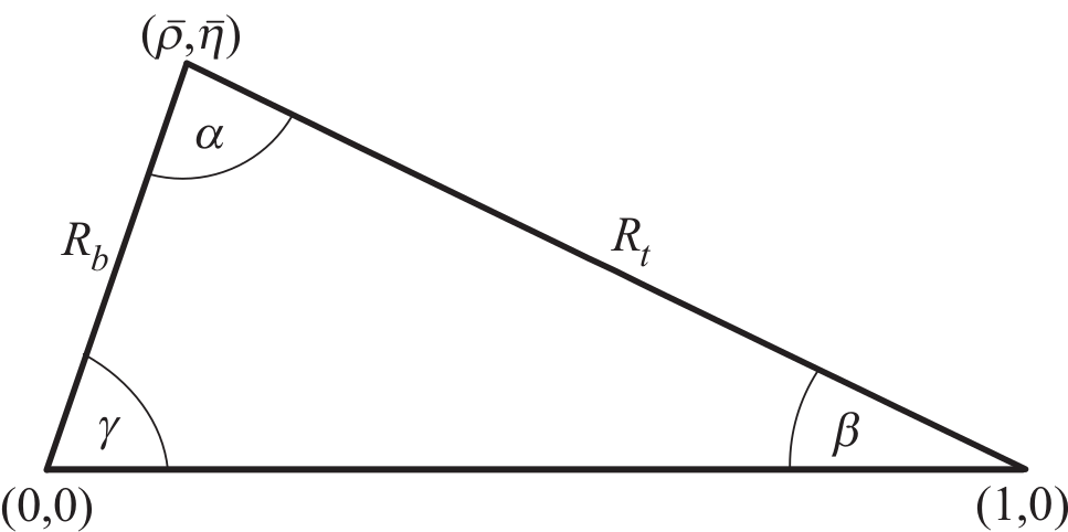
Figure 1: The Unitarity Triangle.

The ratios $R_{i}(\beta,\gamma)$ within the SM are given below. The explicit expressions for these ratios as functions of $\beta$ and $\gamma$ are given in Buras:2021nns . Here we just list the final results using the CKM parameters in (19) which were not given there. Moreover in the case of the ratios $R_{5}$ and $R_{7}$ we use the most recent results for the formfactors entering $\mathcal{B}(B^{+}\to K^{+}\nu\bar{\nu})$ from the HPQCD collaboration Parrott:2022zte ; Parrott:2022rgu . Here we go.

$$\boxed{R_{0}(\beta)=\frac{\mathcal{B}(K^{+}\rightarrow\pi^{+}\nu\bar{\nu})}{\mathcal{B}(K_{L}\rightarrow\pi^{0}\nu\bar{\nu})^{0.7}}={(2.03\pm 0.11)}\times 10^{-3}\,,}$$ (6)

$$\boxed{R_{\rm SL}=\frac{\mathcal{B}(K_{S}\to\mu^{+}\mu^{-})_{\rm SD}}{\mathcal{B}(K_{L}\rightarrow\pi^{0}\nu\bar{\nu})}=(6.29\pm 0.52)\times 10^{-3}\,,}$$ (7)

$$\boxed{R_{1}(\beta,\gamma)=\frac{\mathcal{B}(K^{+}\rightarrow\pi^{+}\nu\bar{\nu})}{\left[{\overline{\mathcal{B}}}(B_{s}\to\mu^{+}\mu^{-})\right]^{1.4}}=53.23\pm 2.75\,,}$$ (8)

$$\boxed{R_{2}(\beta,\gamma)=\frac{\mathcal{B}(K^{+}\rightarrow\pi^{+}\nu\bar{\nu})}{\left[{\mathcal{B}}(B_{d}\to\mu^{+}\mu^{-})\right]^{1.4}}=(8.37\pm 0.47)\times 10^{3}\,,}$$ (9)

$$\boxed{R_{3}(\beta,\gamma)=\frac{\mathcal{B}(K_{L}\rightarrow\pi^{0}\nu\bar{\nu})}{\left[{\overline{\mathcal{B}}}(B_{s}\to\mu^{+}\mu^{-})\right]^{2}}=(2.06\pm 0.16)\times 10^{6}\,,}$$ (10)

$$\boxed{R_{4}(\beta,\gamma)=\frac{\mathcal{B}(K_{L}\rightarrow\pi^{0}\nu\bar{\nu})}{\left[{\mathcal{B}}(B_{d}\to\mu^{+}\mu^{-})\right]^{2}}=(2.83\pm 0.24)\times 10^{9}\,,}$$ (11)

$$\boxed{R_{5}(\beta,\gamma)=\frac{\mathcal{B}(K^{+}\rightarrow\pi^{+}\nu\bar{\nu})}{\left[\mathcal{B}(B^{+}\to K^{+}\nu\bar{\nu})\right]^{1.4}}={(2.32\pm 0.13)\times 10^{-3}\,,}}$$ (12)

$$\boxed{R_{6}(\beta,\gamma)=\frac{\mathcal{B}(K^{+}\rightarrow\pi^{+}\nu\bar{\nu})}{\left[\mathcal{B}(B^{0}\to K^{0*}\nu\bar{\nu})\right]^{1.4}}=(8.43\pm 1.21)\times 10^{-4}\,,}$$ (13)

$$\boxed{R_{7}=\frac{\mathcal{B}(B^{+}\to K^{+}\nu\bar{\nu})}{{\overline{\mathcal{B}}}(B_{s}\to\mu^{+}\mu^{-})}={(1.30\pm 0.07)\times 10^{3}\,,}}$$ (14)

$$\boxed{R_{8}=\frac{\mathcal{B}(B^{0}\to K^{*0}\nu\bar{\nu})}{{\overline{\mathcal{B}}}(B_{s}\to\mu^{+}\mu^{-})}=(2.68\pm 0.25)\times 10^{3}\,.}$$ (15)

4 New Look at the CKM Matrix and $|V_{cb}|-\gamma$ Plots

Let us emphasize that our strategy uses as basic CKM parameters Blanke:2018cya ; Buras:2022wpw ; Buras:2021nns ; Buras:2022qip

$$|V_{us}|=\lambda,\qquad|V_{cb}|,\qquad\beta,\qquad\gamma,$$ (16)

with $\beta$ and $\gamma$ being the two angels of the UT shown in Fig. 1.

This differs from the standard parametrization of the CKM matrix that involves three real parameters and one complex phase

$$s_{12}=|V_{us}|,\qquad s_{13}=|V_{ub}|,\qquad s_{23}=|V_{cb}|,\qquad\gamma,$$ (17)

that can be determined separately in tree-level decays. Consequently, basically all flavour phenomenology in the last three decades used this set of parameters. In particular the determination of the UT was dominated by the measurements of its sides $R_{b}$ and $R_{t}$ through tree-level $B$ decays and the $\Delta M_{d}/\Delta M_{s}$ ratio, respectively, with some participation of the measurements of the angle $\beta$ through the mixing induced CP-asymmetries like $S_{\psi K_{S}}$, the parameter $\varepsilon_{K}$ and much less precise angle $\gamma$. This is the case not only of global analyses by UTfitterBona:2007vi and CKMfitter Charles:2004jd but also of less sophisticated determinations of the CKM matrix and of the UT.

However, as pointed out in Buras:2022wpw ; Buras:2021nns ; Buras:2022qip , the most powerful strategy appears eventually to be the one which uses as basic CKM parameters the ones in (16), that is two mixing angles and two phases. This choice is superior to the one in which $\beta$ is replaced by $|V_{ub}|$ for several reasons:

• The known tensions between exclusive and inclusive determinations of $|V_{cb}|$ and $|V_{ub}|$ Finauri:2023kte ; FlavourLatticeAveragingGroupFLAG:2021npn are represented only by $|V_{cb}|$ which can be eliminated efficiently by constructing suitable ratios of flavour observables $R_{i}(\beta,\gamma)$, see previous section, which are free of the tensions in question.

• As pointed out already in 2002 Buras:2002yj , the most efficient strategy for a precise determination of the apex of the UT, that is $(\bar{\varrho},\bar{\eta})$, is to use the measurements of the angles $\beta$ and $\gamma$. Indeed, among any pairs of two variables representing the sides and the angles of the UT that are assumed for this exercise to be known with the same precision, the measurement of $(\beta,\gamma)$ results in the most accurate values of $(\bar{\varrho},\bar{\eta})$. The second best strategy would be the measurements of $R_{b}$ and $\gamma$. However, in view of the tensions between different determinations of $|V_{ub}|$ and $|V_{cb}|$, that enter $R_{b}$, the $(\beta,\gamma)$ strategy will be a clear winner once LHCb and Belle II collaborations will improve the measurements of these two angles.

• The $|V_{cb}|-\gamma$ plots for fixed $\beta$, proposed in Buras:2022wpw ; Buras:2021nns are, as emphasized in Buras:2022nfn , useful companions to common unitarity triangle fits because they exhibit better possible inconsistences between $|V_{cb}|$ and $(\beta,\gamma)$ determinations than the latter fits. We will demonstrate this below.

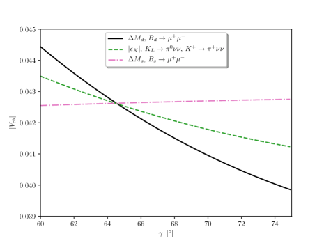
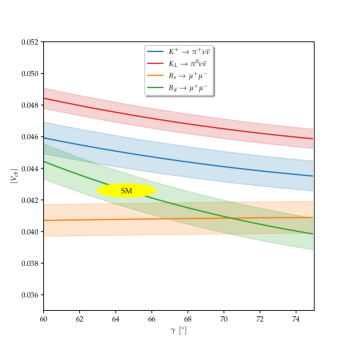
Figure 2: Left:Schematic illustration of the action of the seven observables in the $|V_{cb}|-\gamma$ plane in the context of the SM. We set $\beta=22.2^{\circ}$ and all uncertainties to zero. Right:The impact of hypothetical future measurements of the branching ratios for $K^{+}\rightarrow\pi^{+}\nu\bar{\nu}$, $K_{L}\rightarrow\pi^{0}\nu\bar{\nu}$, $B_{d}\to\mu^{+}\mu^{-}$ and $B_{s}\to\mu^{+}\mu^{-}$ on the $|V_{cb}|-\gamma$ plane. All uncertainties are included. The yellow disc represents the SM as obtained in (19). From Buras:2022nfn .

In this context let us present two simple formulae that are central in the $(\beta,\gamma)$ strategy as they allow to calculate the appex of the UT in no time, but to my knowledge they have been presented only recently for the first time Buras:2023qaf . They read

$$\boxed{\bar{\varrho}=\frac{\sin\beta\cos\gamma}{\sin(\beta+\gamma)},\qquad\bar{\eta}=\frac{\sin\beta\sin\gamma}{\sin(\beta+\gamma)}.}$$ (18)

Evidently they can be derived by high-school students, but the UT is unknown to them and somehow no flavour physicist got the idea to present them in print until its first appearance in Buras:2023qaf .

The superiority of the $|V_{cb}|-\gamma$ plots with respect to $|V_{cb}|$ and $\gamma$ over UT plots has been emphasized in Buras:2022nfn . Indeed,

• They exhibit $|V_{cb}|$ and its correlation with $\gamma$ determined through a given observable in the SM, allowing thereby monitoring the progress on both parameters expected in the coming years. Violation of this correlation in experiment will clearly indicate NP at work.

• They utilize the strong sensitivity of rare $K$ decay processes to $|V_{cb}|$ thereby providing precise determination of $|V_{cb}|$ even with modest experimental precision on their branching ratios.

• They exhibit, as shown in Fig. 2, the action of $\Delta M_{s}$ and of $B_{s}$ decays, like $B_{s}\to\mu^{+}\mu^{-}$ which is not possible in the common UT-plot.

• Once the accuracy of $\gamma$ measurements will approach $1^{\circ}$ it will be easier to monitor this progress on the $|V_{cb}|-\gamma$ plot than on the UT-plot.

In Fig. 2 we show examples of such plots that can be used in the search for new animalcula. See figure caption for explanations.

5 CKM Parameters

As the rapid test for the $\Delta F=2$ observables turned out to be negative we can now determine the CKM parameters using these observables without NP infection. We find Buras:2022wpw

$$\boxed{|V_{cb}|=42.6(4)\times 10^{-3},\quad\gamma=64.6(16)^{\circ},\quad\beta=22.2(7)^{\circ},\quad|V_{ub}|=3.72(11)\times 10^{-3}\,}$$ (19)

and consequently

$$\boxed{|V_{ts}|=41.9(4)\times 10^{-3},\qquad|V_{td}|=8.66(14)\times 10^{-3}\,,\qquad{\rm{Im}}\lambda_{t}=1.43(5)\times 10^{-4}\,,}$$ (20)

$$\boxed{\bar{\varrho}=0.164(12),\qquad\bar{\eta}=0.341(11)\,,}$$ (21)

where $\lambda_{t}=V_{ts}^{*}V_{td}$. Note that our result for $\gamma$ agrees perfectly with the most recent LHCb measurement: $\gamma=64.6(28)^{\circ}$.

Decay	SM Branching Ratio	Data
$B_{s}\to\mu^{+}\mu^{-}$	$(3.78^{+0.15}_{-0.10})\cdot 10^{-9}$	$(3.45\pm 0.29)\cdot 10^{-9}$ HFLAV:2022pwe
$B_{d}\to\mu^{+}\mu^{-}$	${(1.02^{+0.05}_{-0.03})}\ \cdot 10^{-10}$	$\leq 2.05\cdot 10^{-10}$ LHCb:2021awg
$B^{+}\to K^{+}\nu\bar{\nu}$	$(4.92\pm 0.30)\cdot 10^{-6}$	$(13\pm 4)\cdot 10^{-6}$ Belle-II:2023esi
$B^{0}\to K^{0*}\nu\bar{\nu}$	${(10.13\pm 0.92)}\cdot 10^{-6}$	$\leq 1.5\cdot 10^{-5}$ Grygier:2017tzo
$K^{+}\rightarrow\pi^{+}\nu\bar{\nu}$	$(8.60\pm 0.42)\cdot 10^{-11}$	$(13.0\pm 3.1)\cdot 10^{-11}$ NA62:2022hqi
$K_{L}\rightarrow\pi^{0}\nu\bar{\nu}$	$(2.94\pm 0.15)\cdot 10^{-11}$	$\leq 2.0\cdot 10^{-9}$ Ahn:2018mvc
$(K_{S}\to\mu^{+}\mu^{-})_{\rm SD}$	$(1.85\pm 0.12)\cdot 10^{-13}$	$\leq 2.1\cdot 10^{-10}$ LHCb:2020ycd

Table 1: Present most accurate SM estimates of the branching ratios for the the magnificant seven obtained using the BV-strategy. The experimental result on $K^{+}\rightarrow\pi^{+}\nu\bar{\nu}$ from NA62 includes the recent data presented in a seminar at CERN.

6 The Magnificant Seven

Until now we dealt only with the issue of the CKM parameters but the choice of the observables that are particularly theoretically clean is also very important. In my view the seven ones listed in Table 1 are particulary promising. We give there their SM values obtained using our strategy together with the present experimental results. Clearly other decays, in particular $B\to K\ell^{+}\ell^{-}$ and $B\to K^{*}\ell^{+}\ell^{-}$, that remain still central in the search for NP, are very important. Unfortunately, there are different views among theorists on the role of long distance QCD effects in these decays and the interpretation of the observed anomalies in these decays is difficult at present.

The strong suppression of NP in $\Delta F=2$ prosesses imposes stringent constraints on the parameter space of $Z^{\prime}$ models and limit their potential effects in rare decays. However, as emphasized in Buras:2014sba ; Buras:2014zga ; Crivellin:2015era , the NP contributions to $\Delta F=2$ processes in these models can be suppressed for a particular pattern of left-handed and right-handed flavour-violating $Z^{\prime}$ couplings so that NP effects in rare K and B decays can be sizable.

The implications of the suppression of NP contributions to $\varepsilon_{K}$ on rare K decays within $Z^{\prime}$ models have been studied in Aebischer:2023mbz . In this case it is sufficient to choose the relevant left-handed couplings to be purely imaginary implying strong correlations between three Kaon decays listed in Table 1 and the ratio $\varepsilon^{\prime}/\varepsilon$ as seen in the left plot in Fig. 3. The strict correlation between $K^{+}\rightarrow\pi^{+}\nu\bar{\nu}$ and $K_{L}\rightarrow\pi^{0}\nu\bar{\nu}$ decays in the presence of strong suppression of NP to $\varepsilon_{K}$ seen in this figure is an example of a general correlation between these decays pointed out by Monika Blanke long time ago Blanke:2009pq . Its version in $Z^{\prime}$ models is presented in the right plot in Fig. 3 taken from Buras:2015yca .

In this context the recent NA62 result for $K^{+}\rightarrow\pi^{+}\nu\bar{\nu}$, listed in Table 1, implies

$$\boxed{R^{+}_{\nu\bar{\nu}}=1.51\pm 0.35\,\qquad(\text{SM}:\leavevmode\nobreak\ R^{+}_{\nu\bar{\nu}}=1).}$$ (22)

making hopes that the branching ratios for $K_{L}\rightarrow\pi^{0}\nu\bar{\nu}$ and $K_{S}\to\mu^{+}\mu^{-}$ could be strongly enhanced over the SM values. However, to this end the experimental error on $K^{+}\rightarrow\pi^{+}\nu\bar{\nu}$ branching ratio should be decreased.

In the case of B decays sufficient suppresion of NP contributions to $\Delta M_{s}$ and $\Delta M_{d}$ requires the presence of both left-handed and right-handed $Z^{\prime}$ couplings to quarks. The corresponding analysis for rare B decays has been performed in Buras:2024new finding again strong correlations between B-decay branching ratios in Table 1 and the ones for $B\to K\ell^{+}\ell^{-}$ and $B\to K^{*}\ell^{+}\ell^{-}$ allowing for the explanation of the anomalies in the latter ones despite the suppression of NP contributions to $\Delta F=2$ processes. In 331 models, in which only left-handed $Z^{\prime}$ couplings are involved, some amount of NP contributions at the level of $5\%$ has to be allowed to explain the anomalies in question Buras:2023ldz .

In the case of decays with neutrinos in the final state the SM predictions are obtained assuming the Dirac nature of neutrinos. However they could be of Majorana type implying different predictions. Moreover, as neutrinos are invisible, what is really measured are the decays $K\to\pi+E_{\rm miss}$ and $B\to K(K^{*})+E_{\rm miss}$ with $E_{\rm miss}$ standing for the missing energy. This means that instead of neutrinos there could be different neutral particles like scalars, fermions and vectors in the final state including dark particles. Strategies for disentangling these possibilities through kinematic distributions in the missing energy $E_{\rm miss}$ have been developed recently in Buras:2024ewl . See also earlier papers listed there. In particular a recent paper on the anatomy of such distributions in $K^{+}\rightarrow\pi^{+}\nu\bar{\nu}$ Gorbahn:2023juq . In fact such a distinction is possible although in many cases it will be a challenge for experimentalists.

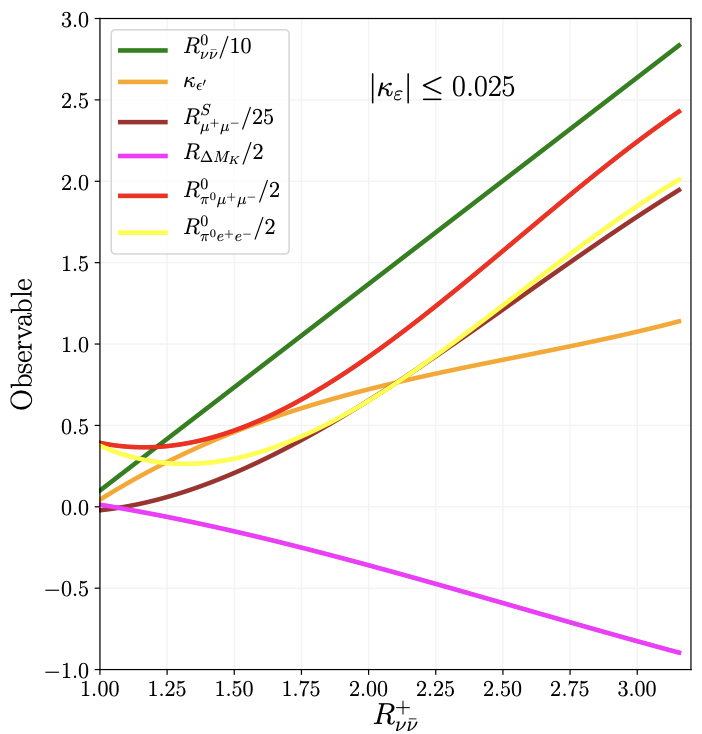
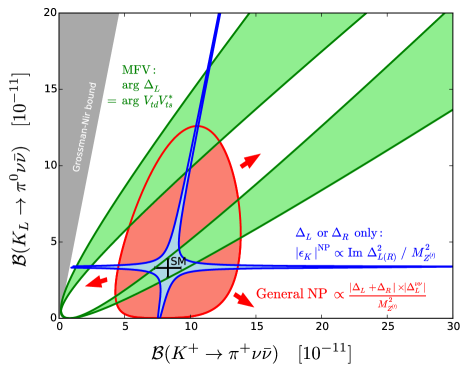
Figure 3: Left:Correlations between the observable $R_{\nu\bar{\nu}}^{+}$ and various other Kaon observables in a $Z^{\prime}$ model. All ratios $R_{i}=1$ in the SM. Note that for $K_{L}\rightarrow\pi^{0}\nu\bar{\nu}$ and $K_{S}\to\mu^{+}\mu^{-}$ the ratios are divided by 10 and 25 respectively. From Aebischer:2023mbz . Right:Correlations between $K^{+}\rightarrow\pi^{+}\nu\bar{\nu}$ and $K_{L}\rightarrow\pi^{0}\nu\bar{\nu}$ in general $Z^{\prime}$ models with green region representing MFV models and blue one coming from $\varepsilon_{K}$ constraint with only LH or RH couplings Blanke:2009pq . From Buras:2015yca .

7 Summary and Shopping List

Despite the presence of various anomalies in the existing data, it is clearly not evident which animalcula could be responsible for them. Possibly, the main candidates are $Z^{\prime}$ vector bosons, leptoquarks and vector-like quarks and vector-like leptons but to find out without any doubts what they are we need more data, in particular for theoretically clean decays as the ones listed in Table 1. Precise measurements of branching ratios for these decays and of various kinematical distributions should allow in this decade to find out which animalcula are responsible for them. The strategies presented here should be helpful in this respect, in particular the ratios $R_{i}(\beta,\gamma)$ listed in Section 3 independenty of whether NP effects are strongly suppressed in $\Delta F=2$ processes or not.

Let me finish this writing with my shopping list for the coming years. I list here only the entries related to flavour physics.

1. Precise measurements of the branching ratios for the magnificant seven and of missing energy distributions for four decays among them. Presently on a forefront are the $B\to K^{(*)}\nu\bar{\nu}$ decays studied intensively by the Belle II experiment Belle-II:2023esi , giving some hints for NP contributions. For selected recent analyses of these data see Bause:2021cna ; He:2021yoz ; Bause:2022rrs ; Becirevic:2023aov ; Bause:2023mfe ; Allwicher:2023syp ; Dreiner:2023cms ; Altmannshofer:2023hkn ; Gabrielli:2024wys ; Hou:2024vyw ; He:2024iju ; Bolton:2024egx ; Marzocca:2024hua ; Allwicher:2024ncl . The same applies to $K^{+}\rightarrow\pi^{+}\nu\bar{\nu}$ for which a very interesting result has been provided very recently by the NA62 experiment listed in Table 1. Taking the present experimental result for $B_{s}\to\mu^{+}\mu^{-}$ allows us to determine the present $|V_{cb}|$-independent experimental values for the the ratios $R_{1}$ and $R_{7}$ in (8) and (14) that read

   $$\boxed{R_{1}=91.4\pm 22.8,\,(\text{SM}:53.23\pm 2.75)}\boxed{R_{7}=(3.8\pm 1.2)\cdot 10^{-3},\,(\text{SM}:(1.30\pm 0.07)\cdot 10^{3}).}$$ (23)

   They differ significantly from very precise SM values. Let us hope that the experimental errors on these ratios will decrease in the coming years.

2. Precise measurements of the branching ratios and of other observables in $B\to K\ell^{+}\ell^{-}$ and $B\to K^{*}\ell^{+}\ell^{-}$ decays and the clarification of the anomalies in them.

3. Precise measurements of $|V_{cb}|$ and $\gamma$ in tree-level decays that would provide additional tests of the BV-strategy.

4. Clarification of anomalies in $B\to\pi K$ decays Buras:2003dj ; Buras:2004ub ; Fleischer:2018bld ; Berthiaume:2023kmp ; Datta:2024zrl ; Szabelski:2024cem .

5. The $\Delta I=1/2$ rule for $K\to\pi\pi$ is almost 70 years old and we do not yet know whether it is fully explained by the SM. The basic QCD dynamics behind this rule - contained in the hadronic matrix elements of current-current operators - has been identified analytically first in 1986 in the framework of the Dual QCD (DQCD) Bardeen:1986vz with some improvements in 2014 Buras:2014maa . This has been confirmed more than 30 years later by the RBC-UKQCD collaboration RBC:2020kdj although the modest accuracy of both approaches still allows for some NP contributions. See Buras:2022cyc for the most recent summary. It would be important to have two lattice calculations with $2+1+1$ flavours.

6. Similar comments apply to $\varepsilon^{\prime}/\varepsilon$ for which the only Lattice QCD calculation is from the RBC-UKQCD with $2+1$ flavours and without isospin breaking effects RBC:2020kdj . Hopefully it will be improved in the coming years and also performed by another QCD lattice collaboration. A stressed in Buras:2023qaf Jean-Marc Gérard and myself expect on the basis of DQCD developed with Bill Bardeen Bardeen:1986vp ; Bardeen:1986uz ; Bardeen:1986vz , significant NP contributions to $\varepsilon^{\prime}/\varepsilon$ that as seen in the left plot in Fig. 3 are consistent with the recent result on $K^{+}\rightarrow\pi^{+}\nu\bar{\nu}$ of the NA62 collaboration.

7. After 37 years of waiting Bardeen:1987vg ; Gerard:2010jt ; Buras:2014maa Lattice QCD confirmed the DQCD claim that the $\hat{B}_{K}\leq 0.75$ with the most accurate result from the RBC-UKQCD collaboration $\hat{B}_{K}=0.7436(82)$ Boyle:2024gge to be compared with $\hat{B}_{K}=0.73\pm 0.02$ from DQCD Buras:2014maa . As the ETM collaboration found $\hat{B}_{K}=0.717(18)(16)$ Carrasco:2015pra it is likely that the central value of $\hat{B}_{K}$ is very close to the DQCD one. This would imply that if there is some small NP contribution to $\varepsilon_{K}$ it must be of the same sign as the SM one. Let us hope that further improvements on $\hat{B}_{K}$ and NP matrix elements Boyle:2024gge ; Buras:2018lgu ; Carrasco:2015pra ; Jang:2015sla will be made in the coming years.

8. Calculation of hadronic matrix elements relevant for $\Delta M_{s}$ and $\Delta M_{d}$ with $2+1+1$ flavours by other lattice QCD collaborations in order to check HPQCD results for these matrix elements.

9. Further search for lepton flavour violation.

We should have then great time in the rest of this decade but unfortunately this does not depend entirely on flavour physicists as we have recently seen in the case of CERN decision on the HIKE experiment. In view of the recent NA62 result on $K^{+}\rightarrow\pi^{+}\nu\bar{\nu}$ this could turn out to be a big mistake.

References

- (1) A.J. Buras, Kaon Theory: 50 Years Later (2023), 2307.15737
- (2) A.J. Buras, J. Girrbach, Rept. Prog. Phys. 77, 086201 (2014), 1306.3775
- (3) A.J. Buras, Gauge Theory of Weak Decays (Cambridge University Press, 2020), ISBN 978-1-139-52410-0, 978-1-107-03403-7
- (4) A.J. Buras (2024), 2403.02387
- (5) A.J. Buras, E. Venturini, Acta Phys. Polon. B 53, A1 (2021), 2109.11032
- (6) A.J. Buras, E. Venturini, Eur. Phys. J. C 82, 615 (2022), 2203.11960
- (7) M. Bona et al. (UTfit), Rend. Lincei Sci. Fis. Nat. 34, 37 (2023), 2212.03894
- (8) J. Charles et al. (CKMfitter Group), Eur. Phys. J. C41, 1 (2005), hep-ph/0406184
- (9) A.J. Buras, Eur. Phys. J. C 83, 66 (2023), 2209.03968
- (10) M. Bordone, B. Capdevila, P. Gambino, Phys. Lett. B 822, 136679 (2021), 2107.00604
- (11) G. Finauri, P. Gambino, JHEP 02, 206 (2024), 2310.20324
- (12) Y. Aoki et al. (Flavour Lattice Averaging Group (FLAG)), Eur. Phys. J. C 82, 869 (2022), 2111.09849
- (13) A.J. Buras, Phys. Lett. B566, 115 (2003), hep-ph/0303060
- (14) R.J. Dowdall, C.T.H. Davies, R.R. Horgan, G.P. Lepage, C.J. Monahan, J. Shigemitsu, M. Wingate, Phys. Rev. D 100, 094508 (2019), 1907.01025
- (15) M. Kirk, A. Lenz, T. Rauh, JHEP 12, 068 (2017), [Erratum: JHEP 06, 162 (2020)], 1711.02100
- (16) D. King, A. Lenz, T. Rauh, JHEP 05, 034 (2019), 1904.00940
- (17) D. King, M. Kirk, A. Lenz, T. Rauh (2019), [Addendum: JHEP 03, 112 (2020)], 1911.07856
- (18) A.J. Buras, Eur. Phys. J. C 82, 612 (2022), 2204.10337
- (19) A.J. Buras, Phys. Rept. 1025, 1 (2023), 1102.5650
- (20) W.G. Parrott, C. Bouchard, C.T.H. Davies (HPQCD), Phys. Rev. D 107, 014511 (2023), [Erratum: Phys.Rev.D 107, 119903 (2023)], 2207.13371
- (21) W.G. Parrott, C. Bouchard, C.T.H. Davies (HPQCD), Phys. Rev. D 107, 014510 (2023), 2207.12468
- (22) M. Blanke, A.J. Buras, Eur. Phys. J. C 79, 159 (2019), 1812.06963
- (23) M. Bona et al. (UTfit), JHEP 0803, 049 (2008), 0707.0636
- (24) A.J. Buras, F. Parodi, A. Stocchi, JHEP 0301, 029 (2003), hep-ph/0207101
- (25) A.J. Buras, M.E. Lautenbacher, G. Ostermaier, Phys. Rev. D50, 3433 (1994), hep-ph/9403384
- (26) L. Wolfenstein, Phys. Rev. Lett. 51, 1945 (1983)
- (27) Y. Amhis et al. (HFLAV) (2022), 2206.07501
- (28) R. Aaij et al. (LHCb), Phys. Rev. D 105, 012010 (2022), 2108.09283
- (29) I. Adachi et al. (Belle-II) (2023), 2311.14647
- (30) J. Grygier et al. (Belle), Phys. Rev. D96, 091101 (2017), [Addendum: Phys. Rev.D97,no.9,099902(2018)], 1702.03224
- (31) M. Zamkovský et al. (NA62), PoS DISCRETE2020-2021, 070 (2022)
- (32) J. Ahn et al. (KOTO), Phys. Rev. Lett. 122, 021802 (2019), 1810.09655
- (33) R. Aaij et al. (LHCb), Phys. Rev. Lett. 125, 231801 (2020), 2001.10354
- (34) A.J. Buras, F. De Fazio, J. Girrbach, Eur. Phys. J. C74, 2950 (2014), 1404.3824
- (35) A.J. Buras, D. Buttazzo, J. Girrbach-Noe, R. Knegjens, JHEP 1411, 121 (2014), 1408.0728
- (36) A. Crivellin, L. Hofer, J. Matias, U. Nierste, S. Pokorski, J. Rosiek, Phys. Rev. D92, 054013 (2015), 1504.07928
- (37) J. Aebischer, A.J. Buras, J. Kumar, Eur. Phys. J. C 83, 368 (2023), 2302.00013
- (38) M. Blanke, Acta Phys.Polon. B41, 127 (2010), 0904.2528
- (39) A.J. Buras, D. Buttazzo, R. Knegjens, JHEP 11, 166 (2015), 1507.08672
- (40) A.J. Buras, P. Stangl (2024), 2411.XXXXX
- (41) A.J. Buras, F. De Fazio, JHEP 03, 219 (2023), 2301.02649
- (42) A.J. Buras, J. Harz, M.A. Mojahed, JHEP 10, 087 (2024), 2405.06742
- (43) M. Gorbahn, U. Moldanazarova, K.H. Sieja, E. Stamou, M. Tabet, Eur. Phys. J. C 84, 680 (2024), 2312.06494
- (44) R. Bause, H. Gisbert, M. Golz, G. Hiller, JHEP 12, 061 (2021), 2109.01675
- (45) X.G. He, G. Valencia, Phys. Lett. B 821, 136607 (2021), 2108.05033
- (46) R. Bause, H. Gisbert, M. Golz, G. Hiller, Eur. Phys. J. C 83, 419 (2023), 2209.04457
- (47) D. Bečirević, G. Piazza, O. Sumensari, Eur. Phys. J. C 83, 252 (2023), 2301.06990
- (48) R. Bause, H. Gisbert, G. Hiller (2023), 2309.00075
- (49) L. Allwicher, D. Becirevic, G. Piazza, S. Rosauro-Alcaraz, O. Sumensari (2023), 2309.02246
- (50) H.K. Dreiner, J.Y. Günther, Z.S. Wang (2023), 2309.03727
- (51) W. Altmannshofer, A. Crivellin, H. Haigh, G. Inguglia, J. Martin Camalich (2023), 2311.14629
- (52) E. Gabrielli, L. Marzola, K. Müürsepp, M. Raidal, Eur. Phys. J. C 84, 460 (2024), 2402.05901
- (53) B.F. Hou, X.Q. Li, M. Shen, Y.D. Yang, X.B. Yuan, JHEP 06, 172 (2024), 2402.19208
- (54) X.G. He, X.D. Ma, M.A. Schmidt, G. Valencia, R.R. Volkas, JHEP 07, 168 (2024), 2403.12485
- (55) P.D. Bolton, S. Fajfer, J.F. Kamenik, M. Novoa-Brunet, Phys. Rev. D 110, 055001 (2024), 2403.13887
- (56) D. Marzocca, M. Nardecchia, A. Stanzione, C. Toni (2024), 2404.06533
- (57) L. Allwicher, M. Bordone, G. Isidori, G. Piazza, A. Stanzione (2024), 2410.21444
- (58) A.J. Buras, R. Fleischer, S. Recksiegel, F. Schwab, Phys. Rev. Lett. 92, 101804 (2004), hep-ph/0312259
- (59) A.J. Buras, R. Fleischer, S. Recksiegel, F. Schwab, Nucl. Phys. B 697, 133 (2004), hep-ph/0402112
- (60) R. Fleischer, R. Jaarsma, E. Malami, K.K. Vos, Eur. Phys. J. C 78, 943 (2018), 1806.08783
- (61) R. Berthiaume, B. Bhattacharya, R. Boumris, A. Jean, S. Kumbhakar, D. London (2023), 2311.18011
- (62) A. Datta, J. Kumar, S. Kumbhakar, D. London (2024), 2408.03380
- (63) A. Szabelski (2024), 2410.16396
- (64) W.A. Bardeen, A.J. Buras, J.M. Gérard, Phys. Lett. B192, 138 (1987)
- (65) A.J. Buras, J.M. Gérard, W.A. Bardeen, Eur. Phys. J. C74, 2871 (2014), 1401.1385
- (66) R. Abbott et al. (RBC, UKQCD), Phys. Rev. D 102, 054509 (2020), 2004.09440
- (67) A.J. Buras, in the Standard Model and Beyond: 2021, in 11th International Workshop on the CKM Unitarity Triangle (2022), 2203.12632
- (68) W.A. Bardeen, A.J. Buras, J.M. Gérard, Phys. Lett. B180, 133 (1986)
- (69) W.A. Bardeen, A.J. Buras, J.M. Gérard, Nucl. Phys. B293, 787 (1987)
- (70) W.A. Bardeen, A.J. Buras, J.M. Gérard, Phys. Lett. B211, 343 (1988)
- (71) J.M. Gérard, JHEP 1102, 075 (2011), 1012.2026
- (72) P.A. Boyle, F. Erben, J.M. Flynn, N. Garron, J. Kettle, R. Mukherjee, J.T. Tsang (RBC, UKQCD), Phys. Rev. D 110, 034501 (2024), 2404.02297
- (73) N. Carrasco, P. Dimopoulos, R. Frezzotti, V. Lubicz, G.C. Rossi, S. Simula, C. Tarantino (ETM), Phys. Rev. D92, 034516 (2015), 1505.06639
- (74) A.J. Buras, J.M. Gérard, Acta Phys. Polon. B 50, 121 (2019), 1804.02401
- (75) B.J. Choi et al. (SWME), Phys. Rev. D93, 014511 (2016), 1509.00592