Query-Efficient Adversarial Attack Against Vertical Federated Graph Learning

Abstract

Graph neural network (GNN) has captured wide attention due to its capability of graph representation learning for graph-structured data. However, the distributed data silos limit the performance of GNN. Vertical federated learning (VFL), an emerging technique to process distributed data, successfully makes GNN possible to handle the distributed graph-structured data. Despite the prosperous development of vertical federated graph learning (VFGL), the robustness of VFGL against the adversarial attack has not been explored yet. Although numerous adversarial attacks against centralized GNNs are proposed, their attack performance is challenged in the VFGL scenario. To the best of our knowledge, this is the first work to explore the adversarial attack against VFGL. A query-efficient hybrid adversarial attack framework is proposed to significantly improve the centralized adversarial attacks against VFGL, denoted as NA², short for Neuron-based Adversarial Attack. Specifically, a malicious client manipulates its local training data to improve its contribution in a stealthy fashion. Then a shadow model is established based on the manipulated data to simulate the behavior of the server model in VFGL. As a result, the shadow model can improve the attack success rate of various centralized attacks with a few queries. Extensive experiments on five real-world benchmarks demonstrate that NA² improves the performance of the centralized adversarial attacks against VFGL, achieving state-of-the-art performance even under potential adaptive defense where the defender knows the attack method. Additionally, we provide interpretable experiments of the effectiveness of NA² via sensitive neurons identification and visualization of t-SNE. The code and datasets are available at https://github.com/hgh0545/NA2.

1 Introduction

Federated graph learning (FGL), a novel distributed learning paradigm, establishes graph neural networks (GNNs) based on distributed data while keeping it decentralized, for the privacy-preserving concern. FGL can be categorized into horizontal FGL (HFGL) and vertical FGL (VFGL) in line with the data distribution characteristic. HFGL [1, 2] is designed for the scenario where clients share the same feature space but different node ID space. Under the vertical setting, VFGL [3, 4] is suitable for the scenario where clients share the same node ID space but different feature space.

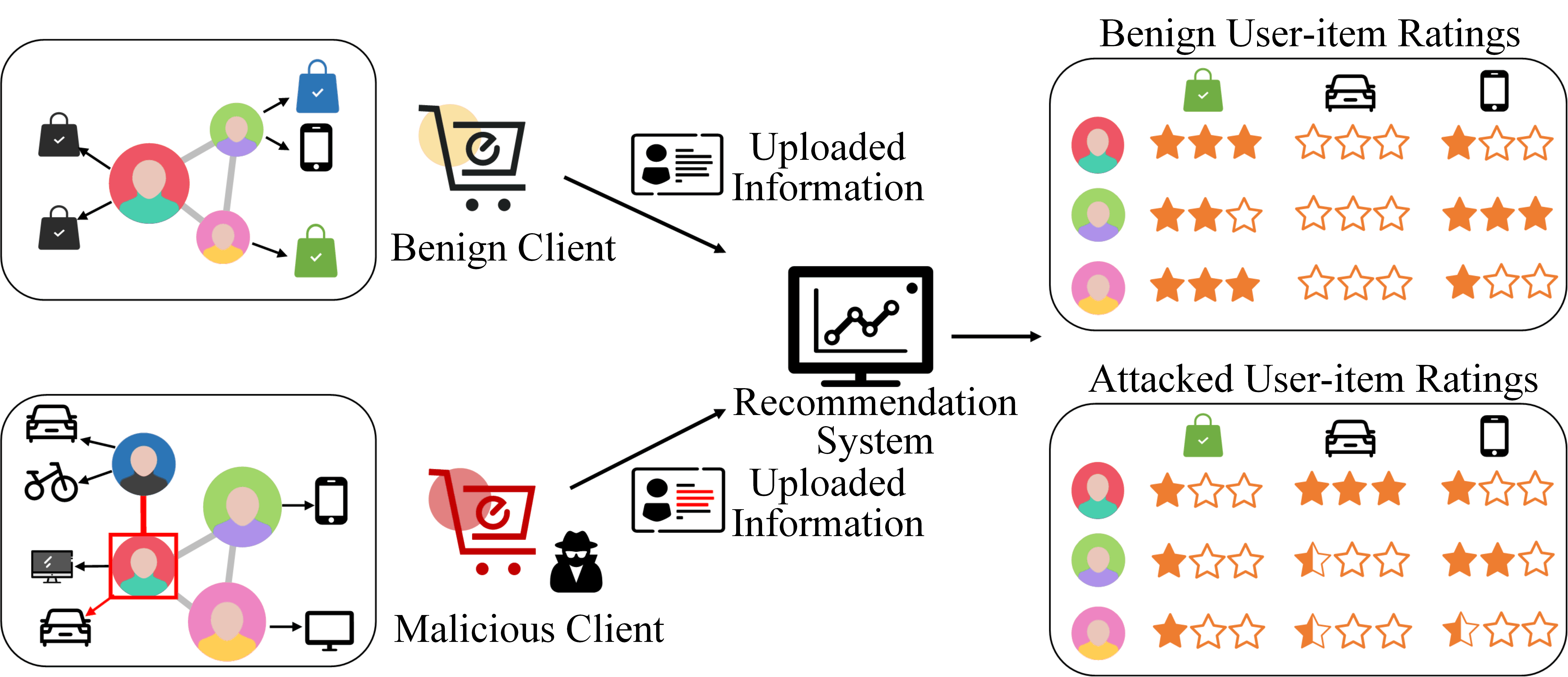
Figure 1: An illustration of the adversarial attack against VFGL in the e-commerce scenario. A small perturbation (e.g., fake friendships, browsing records) may mislead the analysis model and cause the wrong recommendation.

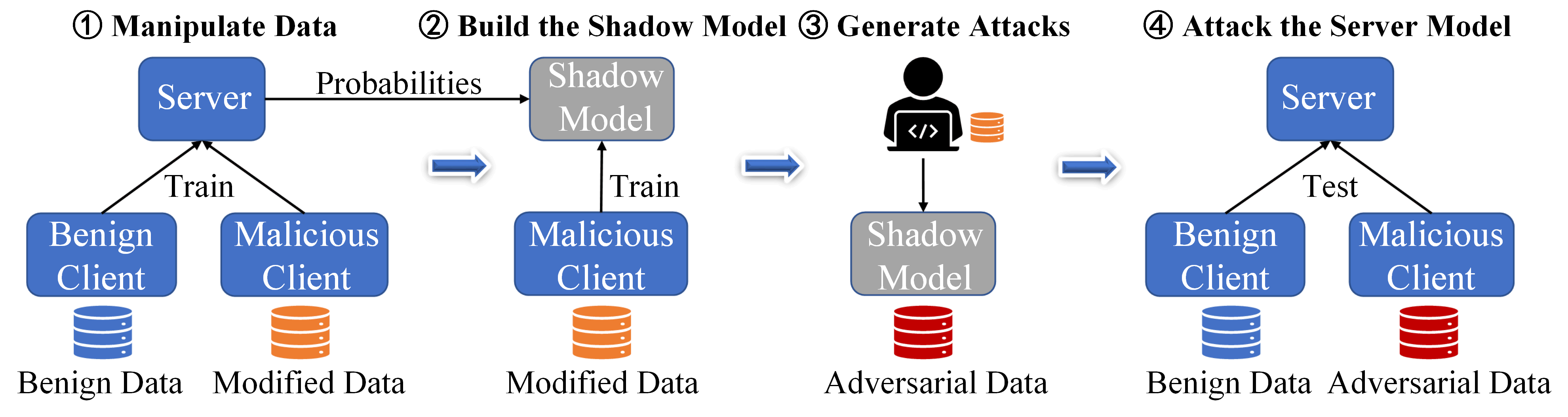
Figure 2: The pipeline of query-efficient hybrid adversarial attack framework against VFGL.

Vertical data distribution is common in practical applications. For example, in electronic commerce, different e-commerce platforms may have the same users, but different attributes space due to the small intersection of the user behaviors over different products and services, such as the consumption behavior or browsing records. It is beneficial for the e-commerce platforms to train a reliable model (i.e., the server model) collaboratively to analyze the users’ behavior and to achieve a win-win situation. VFGL is suitable for such a practical scenario, where the data can be constructed into graphs without sharing sensitive data.

In such a practical application, there is still a potential threat in VFGL, i.e., it may be exposed to the threat of adversarial attacks. Fig. 1 shows the threat model in a practical scenario. Some dishonest e-commerce platforms may manipulate the data for the purpose of unfair competition. For example, adversarial attacks cause other cooperative clients to obtain incorrect predictive feedback when accessing the server model (e.g., modeling the user interest) in VFGL. As a result, erroneous predictions of the users’ interests may degrade the counterparty’s recommendation system.

In this work, we focus on exploring the vulnerability of VFGL to adversarial attacks. Numerous adversarial attacks have been proposed against the centralized GNN (i.e., the GNN with centralized data), including white-box attacks [5, 6, 7], gray-box attacks [8, 9] and black-box attacks [10, 11, 12, 13]. Although these attacks conduct successful attacks on the centralized GNN, they are all challenged in VFGL scenarios. The white-box and gray-box attacks are not applicable to VFGL, since they require the knowledge of the target model’s structure, parameters, or both. However, the malicious client in VFGL does not have access to the server model which makes the final decision. For black-box attacks, one of the mainstream methods is constructing a shadow model, use the shadow model to generate adversarial examples, then transfer them to the target model. Another type is implemented by optimizing adversarial examples evaluated by the feedback of the target model. The latter relies on a large number of queries to the server model, which incurs high query costs and increases the risk of being detected. Thus, we select to build the shadow model as the strategy for adversarial attacks against VFGL.

In summary, there are some challenges for adversarial attacks against VFGL. (i) Knowledge Limitation: It requires constructing successful attacks without any structure or parameter details of the server model. (ii) Query Limitation: The queries for prediction results from the server should be limited for stealthiness. To address these challenges, we propose an adversarial attack framework against VFGL through a four-stage pipeline, shown in Fig. 2. To tackle challenge (i), we construct a reliable shadow model during the training process. The training data of the local client remains private to the server and other clients, the malicious client can manipulate it to make the server model more dependent on the malicious client’s local data, which is beneficial to use the malicious client’s local data to train a shadow model similar to the server model. Thus, the adversary can use the shadow model to generate adversarial examples without query from the server, to address challenge (ii).

The contributions of this work are summarized as follows:

• To the best of our knowledge, this is the first work of adversarial attack against VFGL. To address the ineffectiveness of centralized attacks against VFGL, we proposed a query-efficient adversarial attack framework, namely NA², which can facilitate a significant improvement for centralized adversarial attacks.

• Inspired by the observation that the server model in VFGL is more likely to be misled by high-contribution clients, a training data manipulation strategy is adopted for NA² to enhance the adversarial attack. Thus, NA² is proposed as a novel hybrid attack, involving training data manipulation, and adversarial attack generation in the testing process.

• By constructing a reliable shadow model in the malicious client, only one query to the server is needed in NA², which makes NA² more efficient and effective.

• Extensive experiments are conducted on five real-world graph-structured datasets, and four advanced adversarial attacks are evaluated in VFGL. The results testify that NA² achieves state-of-the-art (SOTA) performance. Besides, NA² still remains a threat to the VFGL with the potential defense mechanism. Furthermore, we interpret the effectiveness of NA² using sensitive neurons identification and visualization of t-SNE.

The rest of the paper is organized as follows. Related works on federated graph learning, adversarial attacks on GNNs and privacy leakage on graph learning are reviewed in Section 2. In Section 3, we present the preliminary and problem formulation. Then, the details of NA² are shown in Section 4, and NA² is evaluated in Section 5. In Section 6, we discuss the limitation of NA², future work and the comparison with the backdoor attacks. At last, the paper is concluded in Section 7.

2 Related Work

Our work focuses on adversarial attacks against privacy-preserving VFGL. In this section, we begin with the existing works of the VFGL, and then the adversarial attacks against GNNs and privacy leakage on graph learning are summarized.

2.1 Adversarial Attacks against GNNs

Numerous studies have shown that GNNs are vulnerable to adversarial attacks, which are well-designed and imperceptible. Based on the attacker’s knowledge and capabilities, the existing works can be divided into white-box attacks, gray-box attacks and black-box attacks.

White-Box Attacks: In white-box settings, the attackers own the parameters of the target model, training data and the ground truth, etc. The gradient-based attack method is a typical white-box attack [5, 7, 14, 6, 15], which applies the gradient information of the target model to generate the adversarial perturbations.

Gray-Box Attacks: For the gray-box settings, the attackers try to train a shadow model to approximate the target model. For instance, Zügner et al. [8] trained a simplified graph convolutional network for Nettack, which computes the misclassification loss sequentially for each edge in the candidate set. Besides, Metattack [9] is proposed based on the meta-gradient of the shadow model.

Black-Box Attacks: In terms of the black-box attacks, reinforcement learning is a typical and widely-used technology. Dai et al. [10] proposed RL-S2V, which applies the reinforcement learning and only requires the prediction labels from the target model. Also, genetic algorithm is applied in the black-box settings where the prediction is available [10]. Ma et al. [13] proposed a reinforcement learning based attack method named RaWatt, which preserves the properties of the graph. Chang et al. [11] proposed GF-Attack, which performs the attack on the graph filter without accessing any knowledge of the target model. Ma et al. [12] extended the common gradient-based attack to black-box settings via the relationship between gradient and PageRank.

The above-mentioned adversarial attack methods are mainly realized by modifying the edges/features of the nodes. Additionally, graph injection attacks are gaining attention. They focus on inject the malicious nodes into the graph rather than modifying the existing edges/features [16, 17, 18].

2.2 Privacy Leakage on Graph Learning

In this paper, the privacy leaked in probabilities (posterior probabilities or confidence scores) is exploited to construct the shadow model. Therefore, we summarize the privacy leakage on FGL. Unfortunately, the research on privacy leakage on FGL [19] is still in its fancy. Thus, the privacy leakage research on GNNs is mainly summarized, as well as existing privacy studies on FGL.

Privacy Leakage on GNNs: Recently, graph neural networks (GNNs) have attracted tremendous attention from both academia and industry [20, 21] ,but GNNs are facing the serious challenge in privacy leakage. According to the goal, it is mainly divided into three main directions [22]: membership inference attack, model extraction attack and model inversion attack. For membership inference attack, Duddu et al. [23] proposed two membership attacks considering white-box and black-box settings. The white-box attack exploits the intermediate low dimensional embeddings, while the black-box one exploits the statistical difference in predictions of the model. He et al. [24] showed that the target nodes with higher subgraph density are easier to perform membership inference, which is caused by the fact that dense subgraphs encourage the target nodes to participate more in the aggregation process of GNN training. Olatunji et al. [25] considered additional structural information is the main reason for GNN privacy leakage. In terms of model extraction, Shen et al. [26] used the accuracy and fidelity to ensure that the shadow model can better imitate the behavior of the target model to achieve the privacy information of the target model. As for model inversion attack, He et al.  [27] first proposed a graph edge stealing method based on the target GNN’s output to infer whether there is an edge connection between any pair of nodes in the graph. GraphMI [22] is proposed to reconstruct the graph considering the properties of the graph including sparsity and feature smoothness. Besides, Zhang et al. [28] systematically studied the privacy leakage problem of graph embeddings, and successfully inferred the basic properties of the target graph, such as the number of nodes, edges, and graph density, etc. Some existing methods rely on obtaining the shadow datasets to build shadow models. However, it is difficult to obtain the shadow datasets with similar distributions to the original datasets in reality (e.g., dimension mismatch due to different class numbers, etc.).

Privacy Leakage on FGL: By sharing model parameters or node embeddings, FGL still suffers the threat of privacy leakage. Some works attempt to apply some privacy-preserving mechanisms to address this issue, such as secure multi-party computation [3, 29], secret sharing [30, 1], differential privacy [31, 32] and homomorphic encryption [4], etc.

2.3 Vertical Federated Graph Learning

Traditional GNNs, which rely on centralized data storage, face systemic privacy risks and high costs. Consequently, they struggle to meet the stringent privacy preservation requirements of modern applications. To address this issue, VFGL has emerged as a promising research area, particularly in vertical data distribution scenarios.

Zhou et al. [3] proposed the first vertical learning paradigm to preserve the privacy, using the secure muti-party computation. Ni et al. [4] applied additively homomorphic encryption in the proposed framework named FedVGCN for node classification task. Besides, VFGL is widely used in practical tasks such as knowledge graph [33] and financial fraud detection [34].

2.4 Attack and Defense in Vertical Federated Learning

Existing attacks on VFL have been shown to undermine model robustness [35]. For instance, some backdoor attacks can mislead the VFL model or damage its overall performance on the original task by designing malicious backdoors. Among them, Liu et al [36] proposed a Label Replacement Backdoor attack (LRB) in which the attacker replaces the gradients of a triggered sample with the ones of a clean sample of the targeted class. Yuan et al [37] introduced the Adversarial Dominating Input (ADI), which is an input sample with features that override all other features and lead to certain model output. As for the adversarial attack against the VFGL, Graph-Fraudster [38] is an attack method that generates adversarial perturbations on the local graph structure to mislead the server model and achieve incorrect predictions. For defense, RVFR [39], a novel framework for robust vertical federated learning, which defends against backdoor and adversarial feature attacks through feature subspace recovery and purification. CAE [40] uses an autoencoder with entropy regularization to disguise true labels, preventing attackers from inferring labels based on batch-level gradients. To further improve robustness, the authors introduce DCAE, which combines CAE with DiscreteSGD to protect against label inference attacks. Unlike the independent feature vectors in VFL, the embeddings of the nodes in the graph are interrelated and interact with each other. Therefore the above defense methods cannot be directly applied to GVFL.

3 Threat Model

Before presenting our method, we give the definition of VFGL, as well as the adversarial attacks on it. Then the threat model is introduced. For convenience, the used definitions of symbols are briefly listed in TABLE 1.

TABLE 1: The definitions of symbols.

Symbol	Definition
$G=(V,E)$	the original graph with sets of nodes and edges
$A,\hat{A}$	the original / adversarial adjacency matrix of $G$
$X,\hat{X},\tilde{X}$	the original / adversarial / manipulated feature matrix of nodes
${f}_{\theta}(\cdot)$	the GNN model with parameter $\theta$
$K$	the number of clients
$\hat{h}_{m}$	the node embeddings of the malicious client
$h_{global},\hat{h}_{global}$	the benign / adversarial global node embeddings
$V_{L}$	the set of nodes with labels
$v_{t}$	the target node to be attacked
$y_{v_{t}}$	the ground truth of the target node $v_{t}$
$Y,Y^{{}^{\prime}}$	the label / probabilities list
$|F|$	the number of class for nodes in the $G$
$\mathcal{S}(\cdot)$	the server model in VFGL
$\mathcal{\tilde{S}}(\cdot)$	the shadow model
$I_{N}$	the identity matrix
$\tilde{D}$	the degree matrix
$H^{l}$	the $l$-th hidden representation of the local GNN
$Z^{l}$	the $l$-th output of the neurons
$W^{l}$	the $l$-th weight matrix of the local GNN
$\tau$	the starting epoch of NA2
$k^{l}$	the index of selected neuron in the GNN’s $l$-th layer
$P_{t}$	the neuron path of the target node $t$ in neuron testing
$C$	the set of the candidate nodes
$I$	the set of the target features
$p$	the probabilities returned by the server model
$B_{\mathcal{V}}$	the decision boundary of the classifier $\mathcal{V}$
$\Delta$	the attack budget for edges modification
$\gamma$	the scale for features modification
$Q$	the query budge for attackers

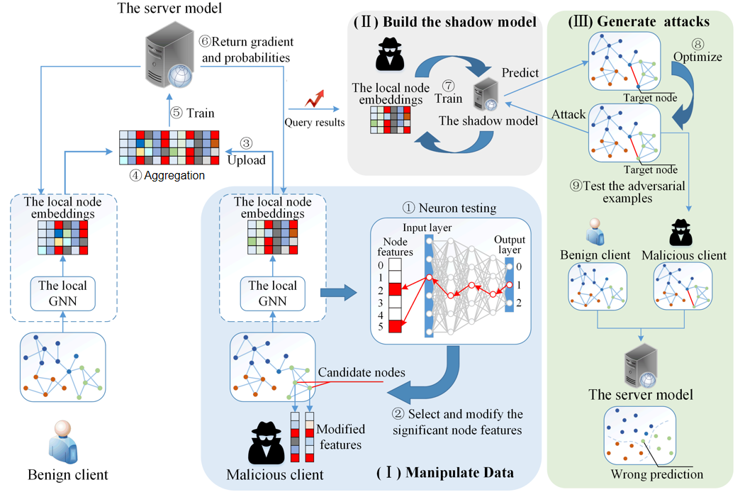
Figure 3: Framework of NA². It can be divided into three stages: (i) Manipulate the local data according to neuron testing results. (ii) Build the shadow model by using the manipulated data. (iii) Generate the adversarial attacks via the shadow model.

Scenario: In this work, a central server model is trained by multiple clients collaboratively in VFGL for node classification. In the training process, the server model issues the prediction and personalized gradient information to each client. During the testing process, the server model only provides the querying service and returns the probability. Besides, in the both training and testing process, the structure and inner parameters of the server model are not revealed to the clients.

Adversary knowledge: Assume that the malicious client only holds its own data (e.g., the adjacency, node features, and the ground truth label of the training nodes), and the information of the local GNN without collecting more extra information from the other clients.

Attack goal: The malicious client aims to mislead the server model by uploading adversarial node embeddings, causing benign clients to receive incorrect predictions. It should be noted that we only consider generating adversarial node embeddings through local GNN instead of constructing fake node embeddings directly because constructing fake node embeddings requires sufficient quality feedback from the server model, which requires multiple queries. Additionally, the preliminaries and problem formulation for Vertical Federated Learning and Adversarial Attacks on Vertical Federated Learning are presented in Appendix A.

4 Methodology

The malicious client can manipulate edges, features, or both. In this work, NA² primarily targets the modification of training node features. This approach is preferred over modifying edges because it impacts a limited subset of features rather than the entire dimension. Consequently, feature modification is a subtler method. In addition, modifying partial but not all the node features can preserve the performance of the main task as much as possible. The proposed NA² follows three stages: (i) Manipulate the local data according to neuron testing results (Section 4.1); (ii) Build the shadow model by using the manipulated data (Section 4.2); (iii) Generate the adversarial attacks via the shadow model (Section 4.3). The overview of NA² is shown in Fig. 3 and the pseudocode is given in Algorithm 1 in the appendix. We detail each step in the following subsections.

4.1 Data Manipulation

To obtain the candidate nodes and features to be modified, the data manipulation is divided into two steps: (i) Locate the significant neural path and obtain the candidate nodes. (ii) Select and modify the target features of the candidate nodes.

4.1.1 Locate Significant Neural Path

NA² commits to locating significant neural paths related to the main task and manipulating the corresponding data, which curbs the performance degradation of the main task as much as possible. First, taking a $L$-layers fully-connected DNN as an example, we give the definition of the neural path as follows.

Definition 1(Significant Neuron Path): The neural path starts from the input neuron, traverses the hidden layer, and ends with the neuron in the output layer. The significant neural path $P$ can be expressed as:

$$P=[k^{1},k^{2},...,k^{L}],$$ (1)

where $k^{1},k^{2},..,k^{L}$ are the any neuron in the $1$-st, $2$-nd, …, $L$-th layer of the DNN, respectively. The neurons in all other layers, except for $k^{L}$, are computed based on the neurons from the previous layer. The specific calculation process is demonstrated by Equation 3 and 4.

Definition 2(Output of the l-th hidden layer in GCN): Then, we introduce the neurons in GNN for a better understanding of NA². Take graph convolutional network (GCN) [41] as an example, the output of the $l$-th hidden layer (without activation function) can be described as:

$$Z^{l}=H^{l+1}=\tilde{D}^{-1/2}(A+I_{N})\tilde{D}^{-1/2}H^{l}W^{l},$$ (2)

where $\tilde{D}$ is the degree matrix of $A+I_{N}$, $I_{N}$ is an identity matrix and $H^{0}=X$. Denote $W\in\mathbb{R}^{N\times M}$, where $N$ is the number of nodes in the graph and $M$ is the number of neurons in the $l$-th hidden layer. Thus, the output of the $i$-th neuron for a node $t$ is the $i$-th column of $Z^{l}_{t}$, which is denoted as $[Z^{l}_{t}]_{i}$.

In order to locate the significant neurons for node classification, this process is performed after training for a number of epochs $\tau$, at which time the corresponding relationship between neurons and downstream tasks is established. More details about the number of epochs $\tau$ will be discussed later. Then, for a $L$-layers GNN, the first neuron of the node $t$ is started with the output layer:

$$k^{l}=\underset{k^{l}}{\mathop{\arg\max}}[|Z_{t}^{l}|]_{k^{l}},$$ (3)

where $|\cdot|$ is the absolute value operator. The $argmax()$ itself is numerically stable because it only performs an index lookup operation, without involving rounding errors in numerical calculations. Even if the elements in the input vector are very close or equal, the function can always accurately return the index of the maximum value.

All neurons on this the significant neuron path are in an active state, and the activation of the end neuron is caused by the activation and “contribution” of other neurons on the path layer by layer. Therefore, we use partial derivatives to measure the “contribution” and lock the key neurons in other layers in reverse order. Thus the rest significant neurons are selected by the following rule:

$$k^{l-1}=\underset{k^{l-1}}{\mathop{\arg\max}}\Big{[}\Big{|}\frac{\partial[Z_{t}^{l}]_{{k}^{l}}}{\partial Z_{t}^{l-1}}\cdot Z_{t}^{l-1}\Big{|}\Big{]}_{k^{l-1}}.$$ (4)

NA² traverses all layers of the local GNN according to the above rule, and finally obtains the node $t$’s reverse neural path $P_{t}=[k^{l},k^{l-1},...,k^{1}]$. Next, the train set is divided according to the node categories. For each category of nodes, we perform neuron tests on them and count the number of nodes with the same neural path. Then, take the neural path with the most nodes as the target path $P_{T}$, and add the rest nodes corresponding to other paths into the candidate nodes set $C$. We use the ReLU function as the activation function. The derivative of ReLU is 1 in the positive interval and 0 in the negative interval. Therefore, the derivative of ReLU is numerically stable and does not exhibit abrupt numerical changes, which prevents the introduction of numerical errors during computation. The stability of the derivative of ReLU ensures that each step in the application of the chain rule is stable, so the process of calculating the partial derivatives in Equation 4 is stable.

4.1.2 Select and Modify the Target Feature

After we have obtained the significant neuron path $P_{T}$, we can identify the significant neuron of the local GNN’s input layer $k^{1}$ by $P_{T}$. Then we extract the $k^{1}$-th column of the weight matrix $W^{1}$ in the first layer of the local GNN, which is denoted as $w_{k}^{1}$. The indexes of the top-${\color[rgb]{0,0,0}B}$ of the $w_{k}^{1}$ are selected within the budget ${\color[rgb]{0,0,0}B}=\gamma\cdot d$ (i.e., the number of features to modify), and they are regarded as the target feature set $I$. $\gamma$ and $d$ are the scale of features modification and the number of node features, respectively. At last, the $i$-th dimension of the candidate nodes’ features are modified as:

$$\begin{split}&\tilde{X}_{c}^{i}=\max(X_{c})\\ s.t.\quad&c\in C\quad and\quad i\in I.\end{split}$$ (5)

The target features are replaced with the maximum value of the original features $X_{c}$, since we believe it maximizes the impact of the examples on the neural path.

Case Study: Equation 5 uses the maximum value for replacement, which might ignore the possibility of outliers. To alleviate this concern, we conducted a comparative experiment. In this work, the SGA is adopted as the perturbation generator, we calculated the variance of all embeddings that need to be modified in the step of modifying node embeddings, and then did not modify the top 5% of the embeddings (called NA2-FGA-N). TABLE 2 records its attack results compared to normal attacks (called NA2-FGA), and the best attack performance highlighted in bold. It is clearly seen that the attack of NA2-FGA is better than NA2-FGA-N on all datasets, indicating that our method remains effective under high variance.

TABLE 2: Comparison of attack success rate between NA2-FGA and NA2-FGA-N for GCN local model.

Local model	Dataset	Attack Method
		NA2-FGA	NA2-FGA-N
GCN	Cora	52%	49%
	Cora ML	67%	63%
	Citeseer	86%	80%
	Pubmed	90%	84%
	ogbn-arxiv	68%	66%

It can be inferred from the above formulas and analysis that neuron testing is a core component of the NA². It analyzes neuron activation to help us identify the key features that have the greatest impact on model decisions. First, neuron testing identifies neural paths closely related to the target task and further screens out the feature subset that has the greatest impact on the key neurons. These features become the targets of data manipulation. By modifying these key features, we can more effectively influence model decisions and thus improve the attack success rate. In addition, neuron testing helps to narrow the scope of data manipulation, avoiding modification of a large number of irrelevant features, thereby improving attack efficiency and reducing the impact on the performance of normal tasks, as well as the risk of being detected. Finally, neuron testing helps us understand the similarity between different model structures, thereby supporting transfer attacks. Even without knowing the structure of the target model, effective attacks can still be carried out.

4.2 Shadow Model Construction

The shadow model refers to a model with similar behavior to the server model, constructed by the malicious client using its own manipulated data and the prediction probabilities returned by the server model. The shadow model acts as a substitute for the server model. It allows the malicious client to generate adversarial embeddings without repeatedly querying the server model, which is both efficient and reduces the risk of detection in the VFGL scenario. First, we construct the shadow model $\tilde{\mathcal{S}}$ by cascading the local GNN and a $L$-layers MLP. Then we query for probabilities $p$ which are used to train the shadow model. The probabilities encapsulate both the main task’s essential information and the server model’s behavior. Thus, we consider the mean square error (MSE) as the target of the shadow model during the training process:

$$\mathcal{L}_{\tilde{\mathcal{S}}}=\frac{1}{R\times|F|}\sum^{R}_{i=1}\sum^{|F|}_{j=1}(\tilde{\mathcal{S}}(A,\tilde{X})-p_{i,j})^{2},$$ (6)

where $R$ is the number of nodes for training the shadow model, and $|F|$ is the number of class for nodes. Since MSE is a convex function and continuously differentiable, its minimum value is the global optimal solution. We can use methods such as gradient descent to minimize MSE, thereby finding the best parameters for the shadow model. Therefore, the optimization process is convergent.

Then we explain why the MSE can be applied to guide the shadow model to mimic the behavior of the server model in VFGL. First, we give the definition of the decision boundary.

Definition 3: The decision boundary of a classifier $\mathcal{V}$ can be expressed as follows:

$$\begin{split}B_{\mathcal{V}}:\quad&\mathcal{V}_{l}(x)-\mathcal{V}_{\hat{l}}(x)=0\\ s.t.&\quad\hat{l}=\underset{l}{\arg}\max\mathcal{V}(x),\end{split}$$ (7)

where $l$ is the $l$-th class of probabilities, and $x$ is the input of the classifier.

Then, the objective of the MSE can be described as:

$$\begin{split}&\underset{\tilde{\mathcal{S}}}{\arg\min}MSE(\tilde{\mathcal{S}}(A,\tilde{X}),\mathcal{S}(h_{global}))\\ &\Leftrightarrow\underset{\tilde{\mathcal{S}}}{\arg\min}|\tilde{\mathcal{S}}(A,\tilde{X})-\mathcal{S}(h_{global})|\\ &\Leftrightarrow\underset{\tilde{\mathcal{S}}}{\arg\min}|(\tilde{\mathcal{S}}_{l}(A,\tilde{X})-\tilde{\mathcal{S}}_{\hat{l}}(A,\tilde{X}))\\ &\quad\quad-(\mathcal{S}_{l}(h_{global})-\mathcal{S}_{\hat{l}}(h_{global}))|\\ &\Leftrightarrow\underset{\tilde{\mathcal{S}}}{\arg\min}|B_{\tilde{\mathcal{S}}}-B_{\mathcal{S}}|.\end{split}$$ (8)

Therefore, using MSE is helpful in fitting the shadow model to the server model. A shadow model that is more similar to the server model can provide more accurate information to the attackers.

4.3 Adversarial Attacks

The shadow model constructed in the above steps can be used for facilitating various centralized attackers to improve the attack success rate. In this work, we consider generating adversarial perturbations by adding/deleting edges in the graph, which is mainstream and effective. The adversarial embeddings for the target node $v_{t}$ produced by the malicious client $m$ are formulated as:

$$\begin{split}&\hat{h}^{v_{t}}_{m}={f}^{m}_{\theta}(\hat{A},\tilde{X},v_{t})\\ &s.t.\quad\hat{A}=ATK(A,\tilde{X},\mathcal{\tilde{S}}),\end{split}$$ (9)

where $ATK(\cdot)$ is a kind of centralized attack method. And the perturbations are limited within the attack budget $\Delta$, i.e., $||\hat{A}-A||_{0}\leq 2\cdot\Delta$. It should be noted that $A$ and $\hat{A}$ are symmetrical in the undirected graph.

5 Experiments

In this section, we conduct experiments to evaluate the effectiveness of NA² and four research questions (RQs) are to be answered:

• RQ1: Can NA² improve the attacks’ performance significantly? What is the query cost of NA²?

• RQ2: Is there a close relationship between the attack success rate and the contribution of the adversary?

• RQ3: Can NA² still work well in defensive VFGL?

• RQ4: How do the scale of modified features and the round of modification affect NA²? What is the time complexity?

5.1 Experimental Settings

5.1.1 Datasets

The proposed method is evaluated on five real-world datasets: Cora [42], Cora_ML [42], Citeseer [42], Pubmed [43] and ogbn-arxiv [44], the information of which is shown in TABLE 3.

To simulate the VFGL learning scenario where clients may not have the same data features, we divide the data and assign them to the clients. However, the graphs in these datasets are sparse, i.e., the average degree is low as shown in TABLE 3. To avoid the appearance of isolated nodes after segmenting the graph, we randomly segment the features only while keeping the edges the same for every client. We test the performance of NA² 5 times as well as other baselines and report the average results to eliminate the impact of the randomness.

TABLE 3: The basic statistics of five graph-structured datasets.

Dataset	#Nodes	#Edges	#Features	#Classes	#Average Degree
Cora [42]	2,708	5,429	1,433	7	2.00
Cora_ML [42]	2,810	7,981	2,879	7	2.84
Citeseer [42]	3,327	4,732	3,703	6	1.42
Pubmed [43]	19,717	44,325	500	3	2.25
ogbn-arxiv [44]	16,9343	1,166,243	128	40	13.7

5.1.2 Local and Shadow Model

Three kinds of GNNs are adopted as the local and shadow model in VFGL.

• GCN [41]: For node classification, a two-layer GCN is applied as the local model in the VFGL. According to Equation 2, the hidden node representation of $(l+1)$-th layer is expressed as:

  $${\color[rgb]{0,0,0}H^{l+1}=\sigma(\tilde{D}^{-1/2}\tilde{A}\tilde{D}^{-1/2}H^{l}W^{l}),}$$ (10)

  where $\sigma$ is the activation function, e.g., ReLU. And $\tilde{A}=A+I_{N}$, $I_{N}$ is unit matrix.

• SGC [45]: SGC removes the nonlinear activation function of GCN, and the forward of SGC is expressed as:

  $${\color[rgb]{0,0,0}H^{l+1}=\tilde{S^{l}}X\tilde{W},}$$ (11)

  where $\tilde{S^{l}}=\tilde{A}\tilde{A}...\tilde{A}$ depends on the layers of SGC, and $\tilde{W}=W^{0}W^{1}...W^{l}$ denotes a collapsed weight matrix.

• GCNII [46]: To address the over-smoothing problem, GCNII adopts initial residual connection and identity mapping, and the node representation is described as:

  $$\scriptsize{\color[rgb]{0,0,0}H^{l+1}=\sigma(((1-\alpha_{l})\tilde{A}H^{l}+\alpha_{l}H^{0})((1-\beta_{l})I_{N}+\beta_{l}W^{l})),}$$ (12)

  where $\alpha_{l}$ and $\beta_{l}$ are hyperparameters to control the scale of input features and adaptive weight decay, respectively. $I_{N}$ is identity matrix for identity mapping.

5.1.3 Evaluation Metrics

To measure the proposed method, attack success rate (ASR), contribution score (CS) and average queries (AQ) are adopted to evaluate the effectiveness and efficiency of NA².

• ASR: The ASR is defined as follows:

  $$ASR=\frac{N_{s}}{N_{a}}\times 100\%,$$ (13)

  where $N_{s}$ is the number of nodes which are attacked successfully, and $N_{a}$ is the number of target nodes.

• CS: Similar to [47], it is a metric to measure the contribution of each client during the training process. The CS of client $i$ is defined as:

  $$\begin{split}&CS_{i}=\frac{con_{i}}{\sum^{K}_{k}con_{k}}\\ s.t.\quad&con_{i}=sinh(\alpha\cdot\frac{acc_{i}}{\sum^{K}_{k}acc_{k}}),\end{split}$$ (14)

  where $acc_{i}$ is the training accuracy of the server model when only $i$’s data is input. $\alpha$ is the scaling constant of contribution. In this work, it is set to 5. $K$ is the number of clients in the VFGL.

• AQ: The AQ is applied to measure the efficiency of the attack, which is defined as:

  $$AQ=\frac{1}{N_{a}}\sum^{N_{a}}_{j}q_{j}.$$ (15)

  If the attack fails, the number of queries $q$ is set to a default query budget $Q$. It should be pointed out that we take the number of times that a malicious client initiates a request to the server model as the number of queries. Frequent requests to the server in a short period of time are suspicious and inefficient. Therefore, the lower the AQ, the higher the efficiency of the attacker.

TABLE 4: The structure and parameters of the local GNN.

Model	#Layers	#Hidden dims	#Out dims	#Training period
GCN	2	32	16	200
SGC	2	32	16	200
GCNII	4	32, 32, 32	16	1,000

5.1.4 Baselines and Adversarial Attacks

Baselines. Due to the lack of research, the proposed NA² is compared with the other two methods we propose:

• Random Features Attack (RFA): It randomly selects the same number of features as NA² for each candidate node, and the value is set to the largest value in the original feature distribution.

• Specific Features Attack (SFA): It randomly selects the same number of features as the specific features set. For each candidate node, the specific features are set to the largest value in the original feature distribution.

For a fair comparison, the number of candidate nodes is the same as NA².

Adversarial attacks. We consider four advanced centralized adversarial attacks FGA [5], GradArgmax [10], Nettack [8], SGA [6] as the attack generator. Moreover, to illustrate the query efficiency of NA², we select a query-based black-box adversarial attack method for comparison. They are briefly described in the appendix B.

5.1.5 Parameter Settings

For different GNNs, the structure and parameters are summarized in TABLE 4. The VFGL is trained using Adam with the learning rate set to 0.01. ReLU is adopted as the activation function for GCN and GCNII. For the malicious client, the scale $\gamma$ for feature modification is searched in [0.01, 0.1], i.e., only $\gamma\cdot d$ ($d$ is the number of node features) features are allowed to be modified per node. For the perturbation generator, the attack budget $\Delta$ is set to 1, considering the sparsity of the graph.

5.1.6 Experimental Environment

Our experimental environment consists of Intel XEON 6240 2.6GHz x 18C (CPU), Tesla V100 32GiB (GPU), 16GiB memory (DDR4-RECC 2666) and Ubuntu 16.04 (OS).

TABLE 5: The average attack success rate ($\pm$ std) and improvement of four adversarial attacks on three kinds of local GNNs.

			Attack Method
			FGA		GradArgmax		Nettack		SGA
Local Model	Dataset	Method	ASR (%)	Impv (%)	ASR (%)	Impv (%)	ASR (%)	Impv (%)	ASR (%)	Impv (%)
		Clean	17.15±2.69	/	8.18±2.57	/	22.55±3.06	/	16.59±2.66	/
		RFA	23.20±4.55	35.28	7.15±3.80	-12.59	28.11±4.09	24.66	22.52±3.19	35.74
		SFA	18.01±1.35	5.01	7.83±3.59	-4.28	22.06±2.76	-2.17	16.64±2.70	0.30
	Cora	NA2	52.37±6.43	205.36	35.55±13.72	334.60	63.35±7.05	180.93	45.01±8.10	171.31
		Clean	12.58±4.83	/	10.95±5.86	/	16.24±6.09	/	10.43±2.88	/
		RFA	23.88±2.74	89.89	16.24±6.09	48.36	18.60±6.67	17.53	13.59±3.18	30.32
		SFA	22.06±4.07	75.41	12.93±6.35	18.13	21.97±5.37	18.12	13.78±2.18	32.14
	Cora_ML	NA2	67.34±6.30	435.50	40.90±17.00	273.67	63.90±13.67	243.55	38.98±14.31	273.80
		Clean	28.53±7.08	/	17.12±5.30	/	30.56±3.84	/	23.94±2.91	/
		RFA	58.97±12.17	106.69	23.68±10.03	38.32	63.34±12.76	107.26	45.17±10.03	88.68
		SFA	28.58±6.01	0.18	14.82±6.12	-13.43	29.82±4.30	-2.42	19.63±4.91	-18.00
	Citeseer	NA2	86.30±4.48	202.49	41.13±13.27	140.25	87.30±2.45	185.67	73.36±8.80	206.43
		Clean	52.50±18.77	/	38.97±24.69	/	48.94±20.75	/	52.74±18.32	/
		RFA	63.45±6.85	20.86	37.56±21.16	-3.61	55.86±16.25	14.16	58.45±12.49	10.83
		SFA	58.38±18.43	11.21	30.82±14.53	-20.92	49.23±18.35	0.60	54.07±17.20	2.52
	Pubmed	NA2	89.90±9.22	65.53	60.71±16.99	55.79	83.47±17.69	70.56	77.28±17.45	51.42
		Clean	33.66±2.25	/	25.65±4.87	/	35.68±2.96	/	39.58±4.32	/
		RFA	28.36±4.23	-15.75	28.36±4.58	10.57	44.24±3.62	23.99	41.23±4.51	4.17
		SFA	35.87±2.58	-6.57	29.58±2.45	15.32	35.35±6.48	-0.92	51.63±4.83	30.44
GCN	ogbn-arxiv	NA2	68.24±4.58	102.73	40.86±5.46	59.30	69.56±6.41	94.96	64.25±2.36	62.33
		Clean	16.27±1.94	/	7.42±5.12	/	23.49±4.95	/	17.84±1.93	/
		RFA	24.01±5.48	47.60	10.96±5.37	47.84	25.85±2.91	10.02	23.67±2.12	32.69
		SFA	17.22±3.62	5.89	7.53±4.34	1.59	22.46±4.29	-4.42	17.96±2.25	0.68
	Cora	NA2	46.41±14.50	185.31	22.42±14.67	202.32	57.26±12.55	143.70	41.43±11.46	132.26
		Clean	22.06±4.71	/	19.21±5.06	/	22.46±3.16	/	12.78±3.10	/
		RFA	41.69±9.82	89.00	27.38±12.04	42.54	40.75±8.83	81.41	23.35±4.18	82.70
		SFA	20.73±4.40	-17.08	17.51±4.57	-11.85	21.44±2.54	6.56	13.19±3.18	-5.69
	Cora_ML	NA2	80.93±6.31	266.87	67.33±12.02	250.56	86.54±3.81	276.32	50.11±15.21	292.16
		Clean	33.17±5.20	/	22.33±5.63	/	33.15±5.87	/	23.60±2.19	/
		RFA	62.91±12.26	110.79	29.56±11.01	32.37	76.75±9.71	131.53	58.38±11.12	147.31
		SFA	27.50±8.23	-6.05	19.69±8.72	-8.85	35.32±7.03	-4.56	22.26±4.62	3.24
	Citeseer	NA2	76.36±15.60	130.22	44.22±23.85	98.01	85.00±7.42	156.41	61.29±9.63	159.65
		Clean	56.68±19.94	/	24.76±22.65	/	53.95±21.09	/	52.38±12.58	/
		RFA	60.40±13.36	6.56	26.52±17.49	7.11	53.59±22.64	-0.68	59.87±11.60	14.30
		SFA	64.20±7.00	13.27	24.10±13.97	-2.65	50.61±21.29	-6.21	52.00±11.59	-0.73
	Pubmed	NA2	76.55±24.88	35.04	54.11±20.00	118.52	79.79±28.70	47.89	73.62±27.30	40.54
		Clean	46.52±13.54	/	28.79±20.31	/	49.67±19.58	/	45.20±22.69	/
		RFA	49.57±8.45	6.56	27.45±6.35	-4.65	55.68±14.56	12.10	49.64±5.96	9.82
		SFA	51.36±7.44	10.40	31.25±5.47	8.54	54.63±8.47	9.99	38.54±5.22	-14.73
SGC	ogbn-arxiv	NA2	68.21±24.80	46.63	42.45±15.41	47.45	63.48±23.85	27.8	58.65±19.42	29.76
		Clean	33.59±14.57	/	28.06±19.28	/	46.89±23.58	/	24.72±5.87	/
		RFA	37.24±16.54	10.88	21.83±16.40	-22.20	52.60±22.35	12.16	37.26±2.24	50.73
		SFA	28.66±14.87	-14.66	20.46±15.71	-27.08	36.96±24.53	-21.19	20.08±4.51	-18.77
	Cora	NA2	62.01±6.33	84.64	31.78±14.59	13.26	75.22±8.93	60.40	51.05±14.25	106.51
		Clean	30.39±9.96	/	23.96±11.30	/	33.64±9.69	/	19.53±5.43	/
		RFA	55.24±17.80	81.79	34.03±20.11	54.22	61.41±13.60	82.55	38.39±10.43	96.59
		SFA	28.60±9.54	-5.87	23.73±9.85	-0.94	36.06±12.51	7.21	17.65±4.55	-9.64
	Cora_ML	NA2	73.51±15.14	141.90	58.92±21.15	145.93	79.28±12.70	135.67	39.58±14.01	102.69
		Clean	40.25±14.41	/	17.21±14.04	/	48.61±13.52	/	37.77±4.36	/
		RFA	58.82±12.63	46.15	29.22±10.59	69.79	69.44±14.60	42.84	57.85±8.63	53.17
		SFA	43.90±19.58	9.08	23.52±17.98	36.70	45.38±21.07	-6.64	37.07±5.11	-1.86
	Citeseer	NA2	69.11±11.53	71.72	32.39±19.53	88.23	78.34±20.46	61.16	61.15±9.60	61.90
		Clean	56.39±18.05	/	41.36±9.10	/	49.26±13.82	/	42.29±6.02	/
		RFA	47.88±11.01	-15.09	32.45±13.45	-21.60	44.76±21.20	-9.14	42.79±6.91	1.18
		SFA	55.92±12.30	-0.84	40.10±7.98	-3.14	56.16±10.98	14.01	45.96±4.22	8.66
	Pubmed	NA2	87.84±8.47	55.77	59.44±14.44	43.59	87.79±7.62	78.21	48.51±8.33	14.71
		Clean	50.84±19.48	/	29.54±8.99	/	35.58±16.25	/	39.59±14.86	/
		RFA	54.36±9.58	6.92	26.58±14.43	-10.02	45.69±8.47	28.41	40.36±8.95	1.95
		SFA	46.58±9.45	-8.38	28.65±12.24	-3.01	39.45±10.68	10.88	45.57±14.33	15.10
GCNII	ogbn-arxiv	NA2	75.85±15.36	49.19	40.98±16.29	38.73	58.87±12.36	65.46	60.23±4.65	52.13

5.2 Effectiveness and Efficiency on Attacking VFGL (RQ1)

In this section, NA² is conducted on five real-world datasets in two scenes, i.e, dual-client-based VFGL and multi-participant-based VFGL. Ablation and transferable experiments are also performed in this section. Besides, the proposed NA² is also compared with the query-based black-box attack regarding the number of queries needed.

TABLE 6: Comparison of attack success rate between NA²-FGA and Graph-Fraudster attack method.

Local Model	Attack Method	Dataset
		Cora	Cora_ML	Citeseer	Pubmed	ogbnn-arxiv
GCN	Graph-Fraudster	40%	28%	51%	69%	58%
	NA2-FGA	52%	67%	86%	90%	68%
SGC	Graph-Fraudster	38%	46%	56%	62%	46%
	NA2-FGA	46%	81%	76%	77%	68%
GCNII	Graph-Fraudster	39%	56%	41%	58%	47%
	NA2-FGA	62%	73%	69%	88%	76%

5.2.1 Attack on Dual-client-based VFGL

As described above, in this scene, the node features are divided into two parts randomly. To verify the generality of NA², we conduct the experiments 5 times and report the ASR with standard deviation. The improvement ratio of ASR ($Impv=(\frac{ASR_{after}}{ASR_{before}}-1)\times 100\%$) is also reported, where $ASR_{before}$ is the ASR without any data manipulation while $ASR_{after}$ is the ASR using NA² or baselines. The results are shown in TABLE 5 and TABLE 6, and the best attack performance is highlighted in bold. Besides, we visualize the neuron’s output (Fig. 4 and 5) to illustrate the effect of NA² on the local GNN. Some observations are concluded in this experiment.

Figure 4: The effect of NA² on the neurons’ activation of the training examples.

Figure 5: The effect of NA² on the neurons’ activation of the benign examples and the adversarial examples.

Figure 6: ASR and CS of NA²-SGA with different number of clients in GCN-based VFGL.

1) NA² can significantly improve the performance of the centralized adversarial attacks and achieves SOTA attack performance compared with baselines. First, analyze the data in TABLE 5. Take FGA on GCN-based VFGL as an example, the Impv of the NA² has reached more than 200% on Cora, Cora_ML and Citeseer, and even achieved a 435.50% attack performance improvement on Cora_ML. Under the same settings, RFA and SFA can only achieve less than 106.69% attack performance improvement. As for Pubmed, the reason why Impv is not obvious is that the attacks have already achieved a high ASR without using any data manipulation method, but NA² still outperforms the baselines. Furthermore, we also note that RFA and SFA may impair attack performance due to their randomness(e.g., attack on GCN-based VFGL using GradArgmax). For the ogbn-arxiv dataset, the attack performance of NA² decreases in comparison to the other four small datasets, but at least it improves the success rate of the attack by 27.8% and still outperforms the baselines. The reason for the decrease in Impv value is that we believe the four attacks we selected, including FGA, are not well-suited for attacking large graph datasets. Therefore, our NA² cannot significantly improve their attack success rate.

Then by analyzing the results from TABLE 6, we observe that NA²-FGA consistently outperforms Graph-Fraudster across all models and datasets, achieving an average attack success rate improvement of 39.46%. The most significant improvement is observed on the Cora_ML dataset, with an increase of 70.00%. We speculate the primary reasons is NA²’s manipulating local training data through the steps of “locating significant neurons path” and “selecting and modifying target features” to increase the contribution of the malicious client. This ensures the server model relies more heavily on the malicious client’s data, resulting in shadow model that more accurately reflects the server model’s behavior and decision boundaries. The accurate shadow model enables NA² to generate adversarial examples that are highly effective in misleading the server model, resulting in a higher attack success rate compared to Graph-Fraudster.

2) Before and after using NA², the activation of neurons to training examples remains similar. We visualized the output of neurons in the last layer of the local GNN for training examples of the same class. As shown in Fig. 4, it can be seen that in the case of normal training, the important neurons for these examples are #9 and #13, and the same after using NA². It indicates that NA² does not introduce large differences on the training set, and it follows the original training process.

3) Neurons’ activation to adversarial examples is changed significantly after using NA². We visualize some nodes that cannot be attacked successfully under clean conditions (i.e., without data manipulation) but succeed under NA². In Fig. 5, for clean conditions, the perturbations at these nodes are not enough to change the activation of neurons, which leads to the failure of the attack. As for NA², compared with the clean case, the distribution of neurons’ activation to benign examples is more concentrated in #9 and #13, which is similar to the case of the training set (Fig. 4). For adversarial examples, the distribution has changed significantly, and it is no longer #9 and #13. It explains why these nodes can be attacked successfully using NA² from the perspective of neurons.

The above experiments suggest VFGL is vulnerable to adversarial attacks as well as the centralized GNNs. Besides, the centralized attacks transferable on VFGL are not as powerful as in the centralized scene. But the threat of these attacks can be improved significantly by adopting NA². Then, the sensitive neurons’ identification shows that the activation shift of neurons is an important factor in attack success.

Figure 7: Transferability and ablation of NA². We present the attack performance (ASR) of nine combinations of the local GNN and the shadow model.

5.2.2 Attack on Multi-client-based VFGL

Considering that a 50% malicious client ratio is not realistic in practical scenarios, a more realistic scenario is considered to evaluate the threat of the proposed NA², i.e., the multi-client-based VFGL. The number of the clients is set in {2, 4, 6, 8, 10}. The node features are split for each client and the structure of the graph is contained as well as the dual-client-based VFGL. The CS of the malicious client and the ASR of NA²-SGA are reported in Fig. 6.

In general, similar results were presented on both large and small datasets is the ASR of all attacks decreases as the number of clients increases, since the impact of adversarial perturbations by the malicious client will gradually decrease. In other words, when the number of clients is large enough, the perturbations of the malicious client will not be enough to confuse the server model. Therefore, improving the contribution of the malicious client to the server model, which makes the server model more dependent on the malicious client’s data, is a feasible measure to improve the attack’s capability in the case of multiple clients. It can be seen that NA² improves the CS of the malicious client and outperforms baselines in general, corresponding to a higher ASR. It is worth noting that in the case of two clients on Cora_ML, although RFA gains a higher CS, the performance of NA²-SGA is still better than RFA-SGA. We believe that it is because the shadow model can be better trained with the data modified by NA² and provides better guidance for attacks. In addition, it can be observed that in the case of eight clients on Pubmed, the performance is better than the case of six clients, which benefits from the higher CS.

In summary, in the multiple clients case, the ASR of attackers shows a downward trend with the increasing number of clients. It is caused by the declining influence of the malicious client. Compared with RFA and SFA, the effect of NA² on the improvement of CS is more obvious, so it can improve ASR more significantly.

5.2.3 Transferability and Ablation of NA²

The transferability and ablation of NA² are evaluated in this subsection. There are nine combinations (i.e., three local models and three shadow models in our experimental configuration) for a given dataset. Besides, to verify the effectiveness of the MSE, the cross entropy loss (CE) calculated from the hard labels of the training set is adopted as a comparison. The experiments are conducted on the Cora dataset and Citeseer dataset. FGA is applied as the attack generator and ASR is used as the metric. The results are shown in Fig. 7.

Transferability: Take NA²-MSE as an example, for GCN and SGC, NA² has a strong transfer attack ability, that is, the shadow model established by GCN/SGC can effectively attack SGC/GCN, due to their similar structure. For GCNII, the transfer attack ability drops subtly, which can be caused by the large structural difference between GCNII and GCN (SGC) and it is difficult to establish a fully consistent shadow model. Compared with the Clean-MSE, in general, NA²-MSE demonstrates stronger transferability (at least 50% ASR is exhibited on both datasets, while this is only 34% at best under Clean-MSE conditions). Similar conclusions can also be obtained in NA²-CE.

Ablation: The proposed NA² consists of two important components, i.e., the data manipulation and the MSE-based shadow model construction. In the ablation experiments, we use these two components as ablation objects.

Take the most general case (i.e., no data manipulation and CE is adopted as the loss function of the shadow model) as the base. Some observations are summarized as follows.

1) The data manipulation enhances the threat of the attack. As shown in Fig. 7, when data manipulation and CE are applied, the ASR is greatly improved in any combination. It is improved from 8% to 29% even in the combination of GCN and GCNII with different structures. We believe this is due to the increased contribution of malicious parties caused by data manipulation. As a result, the perturbation has a greater impact on the server model.

TABLE 7: Comparison of attack success rate and the average number of queries between NA²-FGA and query-based black-box attack method. There are 100 examples randomly selected for the evaluation.

Local Model	Attack Method	Dataset
		Cora		Cora_ML		Citeseer		Pubmed
		ASR	AQ	ASR	AQ	ASR	AQ	ASR	AQ
GCN	GeneticAlg	9%	182.38	3%	194.06	4%	188.07	8%	184.49
	NA2-FGA	51%	1.00	72%	1.00	82%	1.00	87%	1.00
SGC	GeneticAlg	10%	180.38	6%	184.23	2%	198.78	5%	190.21
	NA2-FGA	45%	1.00	37%	1.00	68%	1.00	74%	1.00
GCNII	GeneticAlg	13%	174.86	4%	192.31	10%	180.45	10%	180.52
	NA2-FGA	45%	1.00	73%	1.00	51%	1.00	88%	1.00

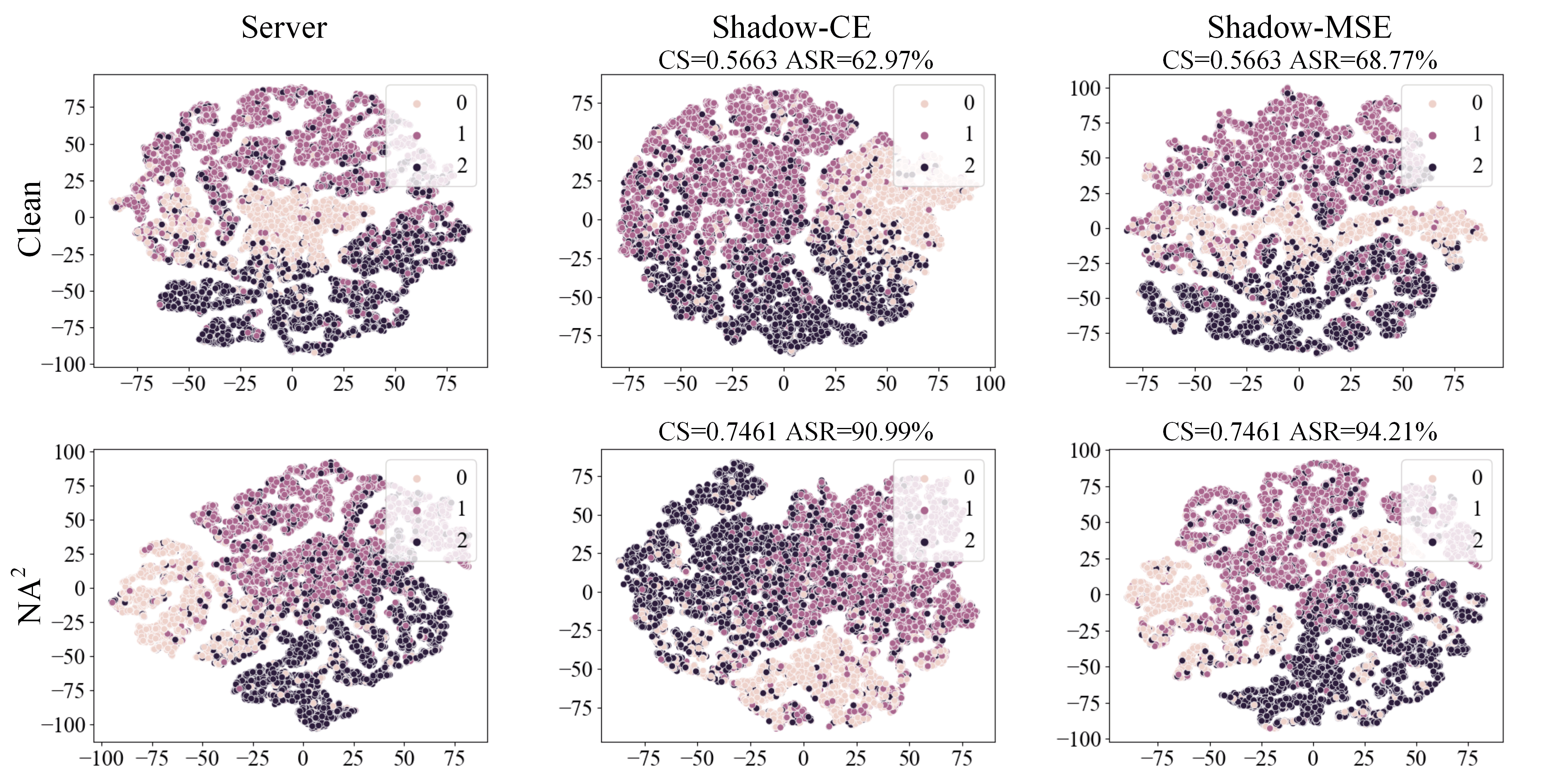
Figure 11: The embeddings which obtained from the server model and the shadow model in the GCN-based VFGL on the Pubmed dataset. They are projected into a 2-dimensional space using t-SNE. The CS and ASR of SGA are reported at the same time.

2) The MSE-based shadow model makes the attack more transferable. While the MSE is adopted without data manipulation, the performance of the attack is slightly improved, and the phenomenon is more obvious in the transfer attack. For example, on the Cora dataset, using GCN as the shadow model to attack, the ASR increases from 8% to 34%. In addition, the improvement is more significant between models with large structural differences, because MSE can effectively utilize the behavioral information leaked by probabilities, which is more conducive to the establishment of the shadow model. To better illustrate it, taking the Pubmed dataset as an example, we project the embeddings extracted from the server model and the shadow model by using t-SNE, which is shown as Fig. 11. It can be observed from the distribution of t-SNE that the distribution using CE is significantly different from the target distribution (Server). It shows that CE only pays attention to the performance but ignores the behavior of the server model. The t-SNE distribution extracted from the shadow model built with NA² using MSE is most similar to the server model with NA². Besides, the CS and ASR (SGA) of the shadow model with NA²-MSE show the best attack performance among all the combinations.

Many existing works [48, 49] use t-SNE to visualize the embeddings in order to explain the effectiveness of the attack methods. Therefore, inspired by this, we use t-SNE for visualization. For NA², the effectiveness of it is closely related to the construction of the shadow model. The higher the similarity between the shadow model and the server’s behavior, the more accurate the information about the server that the shadow model provides to the attacker, and NA² performs better. That’s why we use t-SNE to visualize the embeddings of the shadow model and server.

In summary, combining the advantages of the above two components (i.e., the data manipulation and the MSE-based shadow model), NA²-MSE achieves SOTA performance in both ASR and transfer attack ability.

5.2.4 Efficiency of Attacking VFGL

In order to verify the query efficiency of NA², we compare NA²-FGA with a query-based black-box attack method, namely GeneticAlg. GeneticAlg is a genetic algorithm-based attack method. The population of GeneticAlg is set to 20, and the number of iterations is set to 10. Thus, the maximum number of queries for a target node is 200. If the attack fails, the number of queries is fixed to 200. TABLE 7 reports the ASR and AQ of NA²-FGA and GeneticAlg on four datasets and three local GNNs.

Since NA²-FGA only needs to initiate one request to the server model to get the probabilities, the number of queries for NA²-FGA is always fixed to 1. As for GeneticAlg, more queries are necessary to optimize the perturbations. Therefore, GeneticAlg has far more queries than NA²-FGA. Besides, in each setting, the ASR of NA²-FGA far exceeds that of GeneticAlg, which shows the superiority of NA²-FGA in attack performance and query efficiency.

In federated learning, stragglers refer to the nodes that take longer to complete the computation tasks compared to other participating nodes. This lag may slow down the training progress of the entire system because the training process usually needs to wait for the computation results from all nodes before it can proceed. Stragglers may appear due to factors such as differences in hardware performance, network delays, and uneven computation loads. However, stragglers will not affect the number of queries for NA². The main reason is that NA²’s queriy occur after the server model has aggregated, i.e., (after all clients have uploaded their local node embeddings). Therefore, NA² can query normally even after stragglers appear, and the number of queries remains 1, with only a delay in the query time.

TABLE 8: Significance analysis among CS (C), MSE (M) and ASR (A).

Percentage	p-value			Correlation Coefficient
	C-M	M-A	C-A	C-M	M-A	C-A
50%	2.2E-11	2.8E-11	2.2E-07	-0.93	-0.75	0.91
25%	2.30E-07	2.60E-07	8.5E-08	-0.58	-0.65	0.87
12.5%	3.4E-04	4.9E-04	4.6E-04	-0.35	-0.45	0.47

5.3 Relationship between the ASR and the Contribution (RQ2)

In this subsection, we perform the significance analysis for the ASR, the MSE and the CS of the malicious client. The correlation coefficient and p-value are adopted as the metrics for the analysis. We set the number of clients to {2, 4, 8} and did three sets of experiments, since there is only one malicious client in our attack method, the percentage of malicious client in the experiments is {50%, 25%, 12.5%}. The analysis are shown in TABLE 8. The analysis is based on GCN-based VFGL on the Cora dataset.

The p-value indicates that there is a strong significance between CS and MSE, MSE and ASR, CS and ASR (the p-value less than 0.05 is significant, and the p-value less than 0.01 is very significant). The correlation coefficient suggests there is a high negative correlation between CS and MSE, MSE and ASR (i.e., the higher the contribution, the better the shadow model can be established with the server, and the shadow model with high similarity can better guide the adversarial attack). And there is a strong positive correlation between CS and ASR, i.e., the VFGL is more likely to be attacked by the high-contribution client.

In addition, from the perspective of the server model, we visualize the weights of the input layer of the server model in dual-client, which is shown in Fig. 8. Since the server model cascades node embeddings from the clients, the weights of the input layer can reflect how dependent the server model is on different clients. $||w_{malicious}||_{2}-||w_{benign}||_{2}$ is used to represent the difference in the model’s dependence on malicious and benign clients, where $||\cdot||_{2}$ is $L2$-norm, $w_{malicious}$ and $w_{benign}$ is the weight of the malicious client and the benign client respectively. $||w_{malicious}||_{2}-||w_{benign}||_{2}$ is improved from 0.0938 to 0.1557 after adopting NA², which indicates the server model is more dependent on the malicious client.

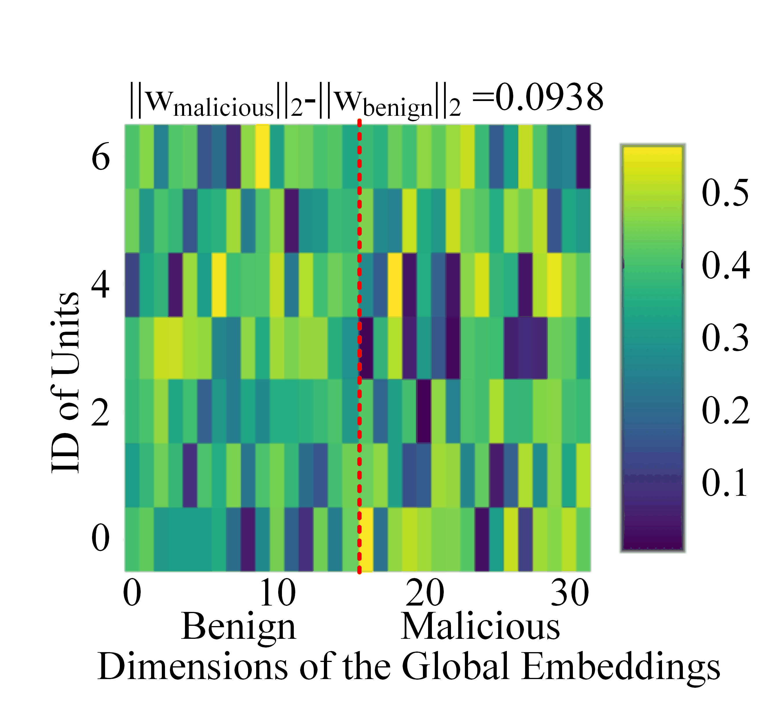
(a) without NA²

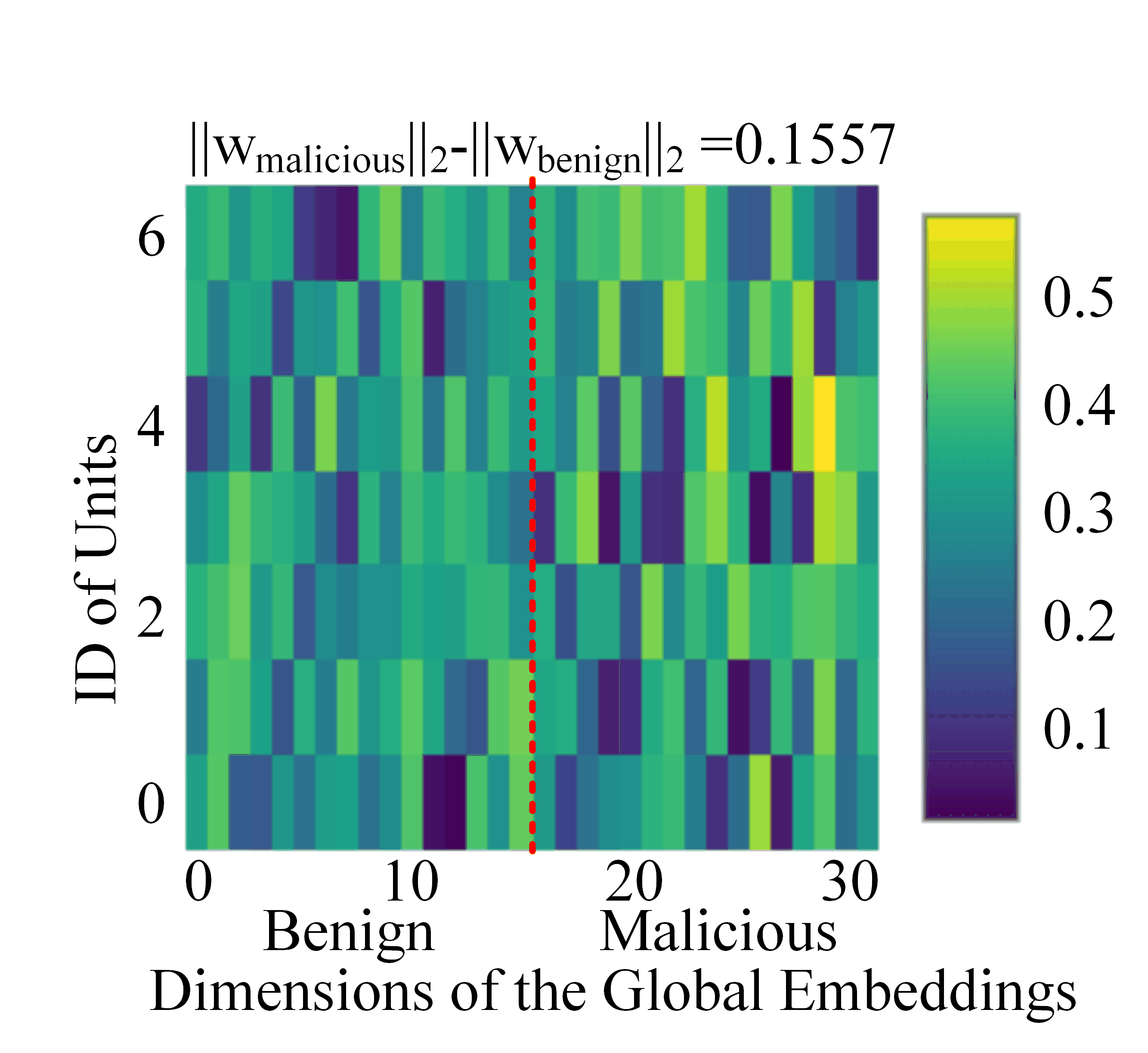
(b) with NA²

Figure 8: Weights distribution of the server’s input layer wo/w NA².

5.4 The Performance of NA² with the Possible Defense (RQ3)

To mitigate the performance of NA², differential privacy (DP) [50] can be adopted as a potential defense method. Unlike approaches such as homomorphic encryption, DP focuses on noise injection on the embeddings rather than encryption in transit, which will be decrypted on the server-side. Therefore, the predicted probabilities of the server model will be changed to weaken the ability of NA² to build the shadow model. In this work, the Laplacian mechanism is used to produce the noises with the scale of noise $\epsilon\in[0,0.5]$. The experiments are validated on Cora and Citeseer, and SGA is selected as the attack generator.

TABLE 9 shows that with the increase of the noise scale, the attack performance of NA²-SGA decreases slightly (within 10%). Besides, injecting large-scale noise will significantly affect the performance of VFGL. For example, when the $\epsilon=0.5$, the accuracy of VFGL dropped by 6.03%, 3.20%, 7.00% and 9.90% on each dataset, respectively. Using DP requires a trade-off between model performance and protection capabilities. In general, DP cannot prevent NA².

In addition to DP, FoolsGold [51] can also be considered as a potential defense method. It measures the similarity between clients by calculating the cosine similarity of historical gradient updates and uses a historical mechanism to track updates from each client. To adapt to the VFL scenario, we require the server to be able to access the gradient information of the client’s model when using FoolsGold. Notably, this change is advantageous to the defender because in the GVFL scenario, the server can only receive embeddings uploaded by the client without gradient information. We set the number of clients to {2, 6, 10} and conducted experiments on four datasets. In the experiments, the attack generator also chose SGA, and the evaluation indicators used were detection rate (DR) and ASR, where DR is the ratio of the number of experiments in which malicious clients were successfully detected to the total number of experiments. The results are shown in TABLE 10.

The results show that the average detection rate of FoolsGold is 8.98%, and the detection rate gradually decreases as the number of clients increases. In addition, the average ASR after defense only decreases by 9.29%, indicating that NA² has good concealment. The core idea of FoolsGold is to distinguish malicious clients from honest clients by utilizing the diversity of client gradient updates. When multiple Sybil clients collaborate in an attack, they share a malicious goal, resulting in more similar gradient updates, which can be identified and weakened by FoolsGold. However, NA² only has one malicious client, and a single malicious client cannot form collaboration with other clients, making it difficult to trigger the detection mechanism of FoolsGold.

5.5 Parameter Analysis and Time Complexity Analysis of NA² (RQ4)

In this subsection, we explore the sensitivity of the feature modification scale $\gamma$ and the starting epoch $\tau$ of data manipulation. In more detail, $\gamma$ is set from 0 to 0.1 with the step size of 0.01, and $\tau$ is set from 0 to 50 with the step size of 5. The experiments are carried out on the Cora dataset. In addition, the time complexity is analyzed and demonstrated with running time experiments.

TABLE 9: The performance of NA²-SGA against the possible defense (DP) on GCN-based VFGL.

Dataset	Metric	$\epsilon$
		0	0.1	0.2	0.3	0.4	0.5
Cora	ACC (%)	76.70	76.80	74.70	74.60	72.90	70.80
	ASR (%)	59.58	49.74	51.67	54.56	56.79	55.65
Cora_ML	ACC (%)	77.90	77.00	74.60	74.30	74.10	74.70
	ASR (%)	51.35	49.74	45.04	47.78	41.57	46.85
Citeseer	ACC (%)	66.80	67.90	66.90	62.40	64.40	59.80
	ASR (%)	85.48	80.27	77.43	87.98	83.23	77.26
Pubmed	ACC (%)	77.70	63.70	69.90	69.90	69.10	67.80
	ASR (%)	94.21	90.58	84.98	88.13	90.45	90.71

TABLE 10: The performance of NA²-SGA against the possible defense ( FoolsGold) on GCN-based VFGL ( The data in the parentheses indicates the ASR when no defense measures are taken).

Dataset	Metric	Number of Client
		2	6	10
Cora	DR (%)	12.76	6.43	3.11
	ASR (%)	49.56(52.37)	25.33(28.21)	27.45(28.51)
Cora_ML	DR (%)	16.18	9.61	4.67
	ASR (%)	60.75(67.34)	31.44(36.12)	11.86(12.45)
Citeseer	DR (%)	13.84	7.29	3.31
	ASR (%)	78.96(86.34)	35.33(39.35)	26.54(26.04)
Pubmed	DR (%)	17.52	8.57	4.47
	ASR (%)	74.58(89.91)	62.58(68.64)	26.97(28.42)

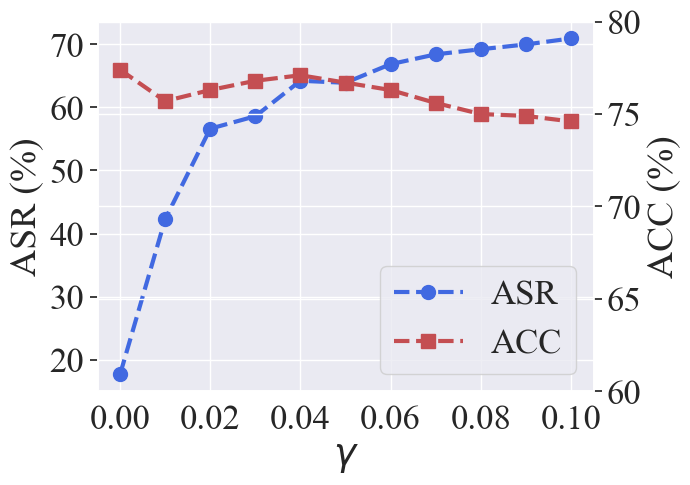
(a) scale of features modification

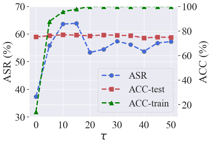
(b) epoch to start NA²

Figure 9: Performance of NA²-FGA on the Cora dataset with different scale of features modification and different epochs to start features modification on GCN-based VFGL.

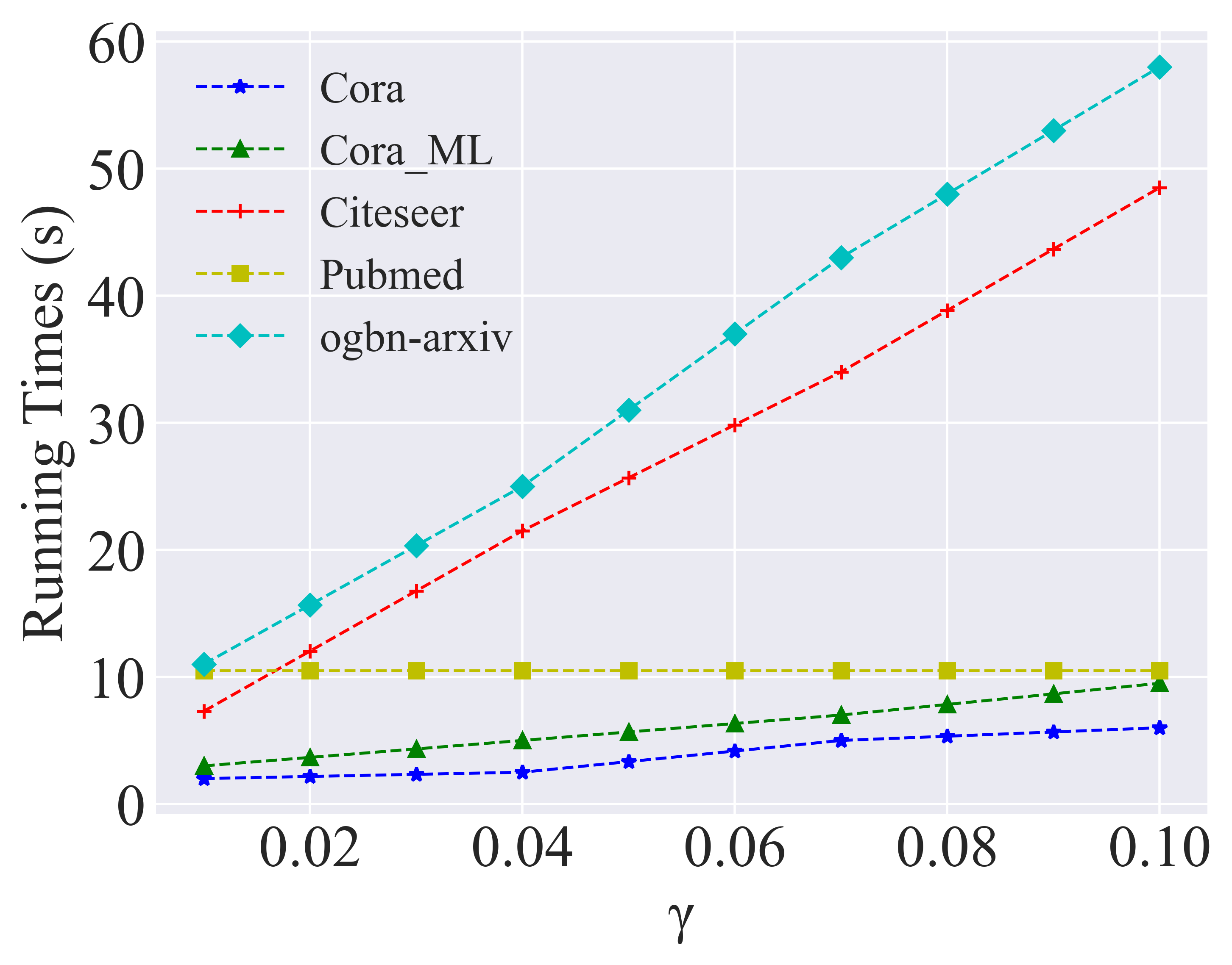
(a) time for data manipulation

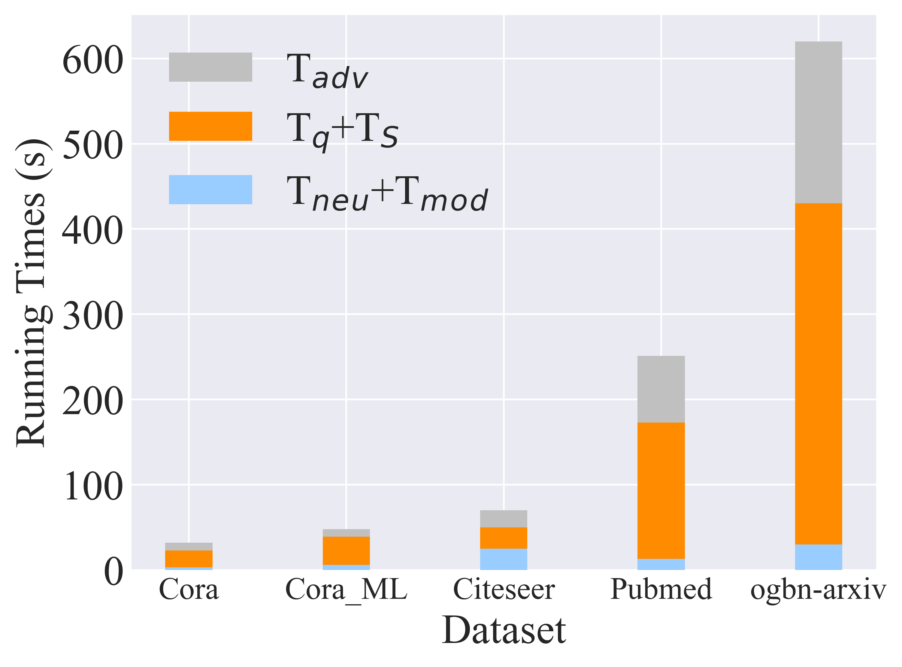
(b) time for each stage of NA²-SGA

Figure 10: Running time of NA².

Parameter analysis: The performance of NA²-FGA is shown in Fig. 9 with the change of the parameters. In Fig. 9(a), it can be observed that the ASR increases gradually with the increase of $\gamma$, and finally tends to be stable. However, it also can be noticed that an excessively large $\gamma$ also affects the benign accuracy of VFGL. For $\tau$, as shown in Fig. 9(b), the ASR rises rapidly in the early stage of training (before $\tau=15$), which may be caused by the uncertainty of important neurons in the early stage. Then, the ASR fluctuates in a small range (within 10%), because the server model has already achieved high accuracy on the training set. In summary, for $\gamma$, we suggest using a moderate value (e.g., 0.05) to trade off the attack performance and the VFGL’s performance. As for $\tau$, data manipulation at an early training stage may affect the attack performance while the model has not started converging.

Time complexity analysis: The time cost of NA² mainly comes from five parts, including the time cost for locating the neurons ($T_{neu}$), the time cost ($T_{mod}$) to modify the features of the candidate nodes, one querying time cost ($T_{q}$), the shadow model’s training time cost ($T_{\tilde{S}}$), and the time cost for the attacker to generate the adversarial perturbations ($T_{adv}$). Therefore, the time complexity of NA² is

$$\small{\mathcal{O}}(T_{neu})+{\mathcal{O}}(T_{mod})+{\mathcal{O}}(T_{q})+{\mathcal{O}}(T_{\tilde{S}})+{\mathcal{O}}(T_{adv})\sim{\mathcal{O}}(N),$$ (16)

where ${\mathcal{O}}(T_{neu})$ depends on the number of the testing examples and the scale of the graph. ${\mathcal{O}}(T_{mod})$ depends on the budget of the modified features, and ${\mathcal{O}}(T_{q})$ is the complexity of the one-querying time. ${\mathcal{O}}(T_{\tilde{S}})$ is the complexity of the training time of the shadow model. ${\mathcal{O}}(T_{adv})$ depends on the adversarial attack methods. Different adversarial scenarios may require different perturbation generators, and the time complexity of different perturbation generators may vary. However, the design of the NA² allows it to adapt to various perturbation generators, so we can maintain the linearity of $T_{adv}$ by choosing an appropriate perturbation generator. Thus, according to all the above steps, ${\mathcal{O}}(N)$ indicates that the time complexity of NA² is linear.

Further, the running time of NA² is tested. As analyzed above, since the shadow model training time cost ($T_{\tilde{S}}$) and the attack generator’s attack time cost ($T_{adv}$) are linear. Compared to other steps, the query time cost ($T_{q}$) is negligibly short. Thus, only the running time of data modification ($T_{neu}+T_{mod}$) is tested, and the results are shown in Fig. 10(a). It can be seen that the running time is linear with the feature modification scale $\gamma$, which is consistent with the analysis of time complexity. It takes more time on the Citeseer dataset because Citeseer has more nodes than Cora and Cora_ML, the number of features is much larger than Pubmed. Besides, the running time for each stage of NA² is shown in Fig. 10(b). The SGA is adopted as the perturbation generator and 100 examples are tested for running time. Obviously, the time consumption for $T_{neu}+T_{mod}$ is the least. We notice that the time cost for the data manipulation on the Citeseer dataset occupies a larger proportion of the total time cost, which is consistent with Fig. 10(a). On the Pubmed dataset, it takes more time to train the shadow model due to its large scale. Furthermore the time complexity of NA² remains linear when using a large dataset ogbn-arxiv. The step of “locating the neuron” involves traversing all layers of the local model for each node according to certain rules. $T_{neu}$ of each node in this step is similar, as the complexity of the graph increases, the total number of nodes increases linearly, so the final time complexity remains linear.

6 Discussion

In this section, we make the discussion about the proposed NA², including limitation, future work and the comparison with the backdoor attacks.

6.1 Limitation and Future Work

Limitation: We test the VFGLs’ accuracy on benign data before and after using NA², the results are reported in TABLE 11. The results show that the performance of VFGL after using NA² decreases slightly. This is understandable that NA² makes server model more dependent on the data from the malicious clients. The data from the benign clients may not be fully utilized, which further causes the decrease of the main task accuracy.

Future work: In future work, we aim to improve the contribution of the malicious client on the premise of making full use of each client’s data to ensure the performance of the main task.

TABLE 11: The accuracy (%) of the VGFL wo/w NA².

Dataset	Local Model
	GCN		SGC		GCNII
	Clean	NA2	Clean	NA2	Clean	NA2
Cora	78.26±0.56	74.24±2.42	78.14±0.97	76.42±1.09	77.18±1.84	74.24±2.32
Cora_ML	81.92±1.17	74.58±2.66	81.78±0.65	75.98±6.23	79.08±1.95	76.06±3.52
Citeseer	65.24±1.25	64.10±2.74	65.24±1.84	62.58±2.14	59.08±2.54	58.18±3.72
Pubmed	77.56±0.71	75.62±3.48	77.70±1.28	73.00±0.10	74.94±1.97	72.76±2.90

6.2 Comparison with the Backdoor Attacks

It is worth noting that NA² is a kind of hybrid attack, which contains the data manipulation in the training process and the adversarial attack in the testing process. In order to distinguish NA² and existing works of backdoor attacks, in this subsection, we discuss the comparison of NA² with the backdoor attacks on GNNs and FL.

Comparison with the backdoor attacks on GNNs: Existing works on graph backdoor [52, 53] focus on injecting backdoors (triggers) into the training data and triggering attacks through the fixed triggers (e.g., fixed subgraphs). Although NA² manipulates the training data, its purpose is to facilitate the adversarial attacks in VGFL scenario where features of the global model are not well known to the malicious client/attacker. The adversarial attack using NA² can be launched using flexible perturbations generated during the inference time, however, the backdoor attack requires a fixed trigger that is embedded during the training.

Comparison with the backdoor attacks on FL: Different from the centralized backdoor attack (CBA) [54] and the distributed backdoor attack (DBA) [55], NA² can leverage diverse adversarial perturbations to achieve attacks on any target example, instead of using fixed local triggers or distributed triggers.

7 Conclusion

In this work, we proposed a query-efficient adversarial attack framework named NA². The proposed NA² uses the key neuron path to locate the key neurons and modifies the corresponding important node features to improve the contribution of the malicious client. A shadow model of the server model is established via the manipulated data and the probabilities returned by the server model. Extensive experiments prove that NA² can improve the performance of the existing centralized adversarial attacks against VFGL significantly, and can achieve SOTA performance. Even with the deployment of the defense mechanism, NA² still achieves impressive attack results. In addition, the sensitive neurons identification and visualization of t-SNE are provided to understand the effectiveness of NA².

Jinyin Chen received BS and PhD degrees from Zhejiang University of Technology, Hangzhou, China, in 2004 and 2009, respectively. She studied evolutionary computing in Ashikaga Institute of Technology, Japan in 2005 and 2006. She is currently a Professor with the Zhejiang University of Technology, Hangzhou, China. Her research interests include artificial intelligence security, graph data mining and evolutionary computing

Wenbo Mu is currently pursuing the masters degree with the college of Information engineering, Zhejiang University of Technology. His research interests include graph data mining and application, and artificial intelligence.

Luxin Zhang is currently pursuing the masters degree with the college of Information engineering, Zhejiang University of Technology. His research interests include graph data mining and application, and artificial intelligence.

Guohan Huang is currently pursuing the master degree with the college of Information engineering, Zhejiang University of Technology. His research interests include graph data mining and applications, and artificial intelligence.

Haibin Zheng is a PhD student at the college of Information Engineering, Zhejiang University of Technology. He received his bachelor degree from Zhejiang University of Technology in 2017. His research interests include deep learning, artificial intelligence, and adversarial attack and defense.

Yao Cheng is currently a senior researcher at Huawei International in Singapore. She received her Ph.D. degree in Computer Science and Technology from University of Chinese Academy of Sciences. Her research interests include security and privacy in deep learning systems, blockchain technology applications, Android framework vulnerability analysis, mobile application security analysis, and mobile malware detection.

Appendix A Preliminary and Problem Formulation

A.1 Vertical Federated Graph Learning

Denote $G=(V,E)$ is the graph with nodes set $V$ and edges set $E$. Define $A$ as the adjacency of the graph and $X$ as the node features. In VFGL, each client maintains the local GNN with its private data and trains the server model collaboratively. It should be noted that in the existing works [3, 4], the edges and node features are split for each client. However, the split subgraph is not in line with the real distribution [56]. Therefore, we consider the setting of dividing only node features but not edges to preserve the original distribution characteristics of the graph. The server aggregates the local node embeddings uploaded by each client. In this work, we consider concatenating the local embeddings as the aggregation strategy:

$$\begin{split}h_{global}&\leftarrow CONCAT(h_{1},...,h_{i},...,h_{K})\\ &s.t.\quad h_{i}={f}^{i}_{\theta}(A_{i},X_{i},V),\end{split}$$ (17)

where $K$ is the number of clients in VFGL, $h_{i}$ is the $i$-th client’s local embeddings produced by the local GNN ${f}^{i}_{\theta}(\cdot)$ with the local private data $(A_{i},X_{i})$.

Then, $h_{global}$ is utilized to train the server model $\mathcal{S}(\cdot)$:

$$\begin{split}\mathcal{L}_{train}&=-\sum_{n=1}^{|V_{L}|}\sum_{l=1}^{|F|}Y_{nl}\ln(Y^{{}^{\prime}}_{nl})\\ &s.t.\quad Y^{{}^{\prime}}=\mathcal{S}(h_{global}),\end{split}$$ (18)

where $V_{L}$ denotes the subset of $V$ labeled with the ground truth, $|F|$ is the number of node classes. $Y$ is the label list, and $Y^{{}^{\prime}}$ is the probabilities list that predicted by the server model. Here, a $L$-layers multilayer perceptron (MLP) is applied as the server model in VFGL in this work.

A.2 Adversarial Attack on Vertical Federated Graph Learning

In the centralized graph learning scenario, the attackers usually reduce the quality of node embeddings to attack the target GNNs by manipulating input data. Likewise, the malicious clients can manipulate the local data and upload the perturbed embeddings to attack the server model with ulterior motives:

$$\begin{split}&\hat{Y}_{t}^{{}^{\prime}}=\mathcal{S}(\hat{h}_{global})\\ s.t.\quad&\hat{h}^{v_{t}}_{global}\leftarrow CONCAT(h^{v_{t}}_{1},...,\hat{h}^{v_{t}}_{m},...,h^{v_{t}}_{K})\\ &\hat{h}^{v_{t}}_{m}={f}^{m}_{\theta}(\hat{A}_{m},\hat{X}_{m},v_{t}),\end{split}$$ (19)

where ${f}^{m}_{\theta}$ is the local GNN of malicious client, $\hat{A}_{m}$ and $\hat{X}_{m}$ are perturbed data. $\hat{h}^{v_{t}}_{m}$ is denoted as the low-quality node embeddings of the target node $v_{t}$, which uploaded by the malicious client.

The target of the malicious client is maximizing the loss of $v_{t}$:

$$\begin{split}&\max\sum\limits_{v_{t}\in T}{{\mathcal{L}_{atk}}(\mathcal{S}(\hat{h}^{v_{t}}_{global}),{{y}_{v_{t}}})}\\ &s.t.\quad\mathcal{L}_{atk}=-\sum_{l=1}^{|F|}Y_{v_{t}l}\ln(Y^{{}^{\prime}}_{v_{t}l}),\end{split}$$ (20)

where $y_{v_{t}}$ is the ground truth of $v_{t}$, and $T$ is the target node set.

Appendix B Adversarial Attacks

• FGA [5]: It constructs the symmetrical edge gradient matrix of the original graph. Then, the maximal absolute edge gradient guides to generate perturbations iteratively.

• GradArgmax [10]: It calculates the gradient of edges based on the loss function, and the greedy algorithm is adopted to select the edges to be modified.

• Nettack [8]: It selects the candidate edges and node features by graph properties (e.g., degree distribution) and generates adversarial perturbations with the highest scoring edges iteratively to fool the classifier.

• SGA [6]: It extracts a subgraph centered at the target node first. Then it generates adversarial attacks by flipping edges with the largest gradient in the subgraph.

To illustrate the query efficiency of NA², we select a query-based black-box adversarial attack method for comparison.

• GeneticAlg [10]: It adopts the genetic algorithm to generate the adversarial perturbations, has to query the target model to calculate the fitness score for each candidate solution that is decided by the population.

Input: Original adjacency $A$, original node features $X$, target node $v_{t}$, starting epoch $\tau$, train set $V_{train}$, attack budget $\Delta$.

Output: The adversarial adjacency $\hat{A}$.

1 Train the VFGL until the starting epoch $\tau$ to start NA².

2 Divided the train set according to the node categories.

3 for $t=1$ to $|V_{train}|$ do

4      Test the train examples according to Equation 3 and 4.

5       Obtain the neuron path $P_{t}$.

6 end for

7Count and select the target path $P_{T}$, and get the candidate nodes set $C$.

8 Identify the significant neuron $k^{1}$ by $P_{T}$, and select the top-$M$ features and the target features set.

9 for $c$ in $C$ do

10      Modify the features of the candidate nodes following Equation 5 and get $\tilde{X}$.

11 end for

12Train the VFGL with the manipulated features $\tilde{X}$ continuously.

13 Query the server model and gain the probabilities $p$.

14 Establish the shadow model $\mathcal{\tilde{S}}$ with the local GNN and a $L$-layers MLP.

15 for t=1 to $T_{shadow}$ do

16       Train $\mathcal{\tilde{S}}$ to minimize the MSE in Equation 6.

17 end for

18Input the original adjacency, the manipulated features $\tilde{X}$ and the shadow $\mathcal{\tilde{S}}$ into the centralized attack method.

19 for i=1 to $\Delta$ do

20      Generate the adversarial adjacency $\hat{A}$ as Equation 9.

21 end for

return the adversarial adjacency matrix $\hat{A}$.

Algorithm 1 NA²

References

- [1] L. Zheng, J. Zhou, C. Chen, B. Wu, L. Wang, and B. Zhang, “Asfgnn: Automated separated-federated graph neural network,” Peer-to-Peer Networking and Applications, vol. 14, no. 3, pp. 1692–1704, 2021.
- [2] B. Wang, A. Li, H. Li, and Y. Chen, “Graphfl: A federated learning framework for semi-supervised node classification on graphs,” arXiv preprint arXiv:2012.04187, 2020.
- [3] J. Zhou, C. Chen, L. Zheng, H. Wu, J. Wu, X. Zheng, B. Wu, Z. Liu, and L. Wang, “Vertically federated graph neural network for privacy-preserving node classification,” arXiv preprint arXiv:2005.11903, 2020.
- [4] X. Ni, X. Xu, L. Lyu, C. Meng, and W. Wang, “A vertical federated learning framework for graph convolutional network,” arXiv preprint arXiv:2106.11593, 2021.
- [5] J. Chen, Y. Wu, X. Xu, Y. Chen, H. Zheng, and Q. Xuan, “Fast gradient attack on network embedding,” arXiv preprint arXiv:1809.02797, 2018.
- [6] J. Li, T. Xie, C. Liang, F. Xie, X. He, and Z. Zheng, “Adversarial attack on large scale graph,” IEEE Transactions on Knowledge and Data Engineering, 2021.
- [7] H. Wu, C. Wang, Y. Tyshetskiy, A. Docherty, K. Lu, and L. Zhu, “Adversarial examples for graph data: deep insights into attack and defense,” in Proceedings of the 28th International Joint Conference on Artificial Intelligence, 2019, pp. 4816–4823.
- [8] D. Zügner, A. Akbarnejad, and S. Günnemann, “Adversarial attacks on neural networks for graph data,” in Proceedings of the 24th ACM SIGKDD International Conference on Knowledge Discovery & Data Mining, 2018, pp. 2847–2856.
- [9] D. Zügner and S. Günnemann, “Adversarial attacks on graph neural networks via meta learning,” arXiv preprint arXiv:1902.08412, 2019.
- [10] H. Dai, H. Li, T. Tian, X. Huang, L. Wang, J. Zhu, and L. Song, “Adversarial attack on graph structured data,” in International conference on machine learning. PMLR, 2018, pp. 1115–1124.
- [11] H. Chang, Y. Rong, T. Xu, W. Huang, H. Zhang, P. Cui, X. Wang, W. Zhu, and J. Huang, “Adversarial attack framework on graph embedding models with limited knowledge,” IEEE Transactions on Knowledge and Data Engineering, 2022.
- [12] J. Ma, S. Ding, and Q. Mei, “Towards more practical adversarial attacks on graph neural networks,” Advances in neural information processing systems, vol. 33, pp. 4756–4766, 2020.
- [13] Y. Ma, S. Wang, T. Derr, L. Wu, and J. Tang, “Graph adversarial attack via rewiring,” in Proceedings of the 27th ACM SIGKDD Conference on Knowledge Discovery & Data Mining, 2021, pp. 1161–1169.
- [14] X. Zang, Y. Xie, J. Chen, and B. Yuan, “Graph universal adversarial attacks: A few bad actors ruin graph learning models,” arXiv preprint arXiv:2002.04784, 2020.
- [15] J. Chen, D. Zhang, Z. Ming, K. Huang, W. Jiang, and C. Cui, “Graphattacker: A general multi-task graph attack framework,” IEEE Transactions on Network Science and Engineering, vol. 9, no. 2, pp. 577–595, 2022.
- [16] Y. Sun, S. Wang, X. Tang, T.-Y. Hsieh, and V. Honavar, “Node injection attacks on graphs via reinforcement learning,” arXiv preprint arXiv:1909.06543, 2019.
- [17] X. Zou, Q. Zheng, Y. Dong, X. Guan, E. Kharlamov, J. Lu, and J. Tang, “Tdgia: Effective injection attacks on graph neural networks,” in Proceedings of the 27th ACM SIGKDD Conference on Knowledge Discovery & Data Mining, 2021, pp. 2461–2471.
- [18] S. Tao, Q. Cao, H. Shen, J. Huang, Y. Wu, and X. Cheng, “Single node injection attack against graph neural networks,” in Proceedings of the 30th ACM International Conference on Information & Knowledge Management, 2021, pp. 1794–1803.
- [19] J. Chen, M. Ma, H. Ma, H. Zheng, and J. Zhang, “An empirical evaluation of the data leakage in federated graph learning,” IEEE Transactions on Network Science and Engineering, vol. 11, no. 2, pp. 1605–1618, 2024.
- [20] B. Wang, B. Jiang, and C. Ding, “Fl-gnns: Robust network representation via feature learning guided graph neural networks,” IEEE Transactions on Network Science and Engineering, vol. 11, no. 1, pp. 750–760, 2024.
- [21] Z. Dong, Y. Chen, T. S. Tricco, C. Li, and T. Hu, “Ego-aware graph neural network,” IEEE Transactions on Network Science and Engineering, vol. 11, no. 2, pp. 1756–1770, 2024.
- [22] Z. Zhang, Q. Liu, Z. Huang, H. Wang, C. Lu, C. Liu, and E. Chen, “Graphmi: Extracting private graph data from graph neural networks,” arXiv preprint arXiv:2106.02820, 2021.
- [23] V. Duddu, A. Boutet, and V. Shejwalkar, “Quantifying privacy leakage in graph embedding,” in Mobiquitous 2020-17th EAI International Conference on Mobile and Ubiquitous Systems: Computing, Networking and Services, 2020, pp. 76–85.
- [24] X. He, R. Wen, Y. Wu, M. Backes, Y. Shen, and Y. Zhang, “Node-level membership inference attacks against graph neural networks,” arXiv preprint arXiv:2102.05429, 2021.
- [25] I. E. Olatunji, W. Nejdl, and M. Khosla, “Membership inference attack on graph neural networks,” arXiv preprint arXiv:2101.06570, 2021.
- [26] Y. Shen, X. He, Y. Han, and Y. Zhang, “Model stealing attacks against inductive graph neural networks,” arXiv preprint arXiv:2112.08331, 2021.
- [27] X. He, J. Jia, M. Backes, N. Z. Gong, and Y. Zhang, “Stealing links from graph neural networks,” in 30th USENIX Security Symposium (USENIX Security 21), 2021, pp. 2669–2686.
- [28] Z. Zhang, M. Chen, M. Backes, Y. Shen, and Y. Zhang, “Inference attacks against graph neural networks,” in Proc. USENIX Security, 2022.
- [29] F. Chen, P. Li, T. Miyazaki, and C. Wu, “Fedgraph: Federated graph learning with intelligent sampling,” IEEE Transactions on Parallel and Distributed Systems, vol. 33, no. 8, pp. 1775–1786, 2021.
- [30] E. Rizk and A. H. Sayed, “A graph federated architecture with privacy preserving learning,” in 2021 IEEE 22nd International Workshop on Signal Processing Advances in Wireless Communications (SPAWC). IEEE, 2021, pp. 131–135.
- [31] C. Zhang, S. Zhang, J. James, and S. Yu, “Fastgnn: A topological information protected federated learning approach for traffic speed forecasting,” IEEE Transactions on Industrial Informatics, vol. 17, no. 12, pp. 8464–8474, 2021.
- [32] C. Wu, F. Wu, Y. Cao, Y. Huang, and X. Xie, “Fedgnn: Federated graph neural network for privacy-preserving recommendation,” arXiv preprint arXiv:2102.04925, 2021.
- [33] M. Chen, W. Zhang, Z. Yuan, Y. Jia, and H. Chen, “Fede: Embedding knowledge graphs in federated setting,” in The 10th International Joint Conference on Knowledge Graphs, 2021, pp. 80–88.
- [34] T. Suzumura, Y. Zhou, N. Baracaldo, G. Ye, K. Houck, R. Kawahara, A. Anwar, L. L. Stavarache, Y. Watanabe, P. Loyola et al., “Towards federated graph learning for collaborative financial crimes detection,” arXiv preprint arXiv:1909.12946, 2019.
- [35] Q. Yang, Y. Liu, Y. Cheng, Y. Kang, T. Chen, and H. Yu, “Vertical federated learning,” in Federated Learning. Springer, 2020, pp. 69–81.
- [36] Y. Liu, Z. Yi, and T. Chen, “Backdoor attacks and defenses in feature-partitioned collaborative learning,” arXiv preprint arXiv:2007.03608, 2020.
- [37] Q. Pang, Y. Yuan, and S. Wang, “Attacking vertical collaborative learning system using adversarial dominating inputs,” arXiv preprint arXiv:2201.02775, 2022.
- [38] J. Chen, G. Huang, H. Zheng, S. Yu, W. Jiang, and C. Cui, “Graph-fraudster: Adversarial attacks on graph neural network-based vertical federated learning,” IEEE Transactions on Computational Social Systems, vol. 10, no. 2, pp. 492–506, 2022.
- [39] J. Liu, C. Xie, K. Kenthapadi, S. Koyejo, and B. Li, “Rvfr: Robust vertical federated learning via feature subspace recovery,” in NeurIPS Workshop New Frontiers in Federated Learning: Privacy, Fairness, Robustness, Personalization and Data Ownership, 2021.
- [40] T. Zou, Y. Liu, Y. Kang, W. Liu, Y. He, Z. Yi, Q. Yang, and Y.-Q. Zhang, “Defending batch-level label inference and replacement attacks in vertical federated learning,” IEEE Transactions on Big Data, 2022.
- [41] T. N. Kipf and M. Welling, “Semi-supervised classification with graph convolutional networks,” arXiv preprint arXiv:1609.02907, 2016.
- [42] A. K. McCallum, K. Nigam, J. Rennie, and K. Seymore, “Automating the construction of internet portals with machine learning,” Information Retrieval, vol. 3, no. 2, pp. 127–163, 2000.
- [43] P. Sen, G. Namata, M. Bilgic, L. Getoor, B. Galligher, and T. Eliassi-Rad, “Collective classification in network data,” AI magazine, vol. 29, no. 3, pp. 93–93, 2008.
- [44] W. Hu, M. Fey, M. Zitnik, Y. Dong, H. Ren, B. Liu, M. Catasta, and J. Leskovec, “Open graph benchmark: Datasets for machine learning on graphs,” Advances in neural information processing systems, vol. 33, pp. 22 118–22 133, 2020.
- [45] F. Wu, A. Souza, T. Zhang, C. Fifty, T. Yu, and K. Weinberger, “Simplifying graph convolutional networks,” in International conference on machine learning. PMLR, 2019, pp. 6861–6871.
- [46] M. Chen, Z. Wei, Z. Huang, B. Ding, and Y. Li, “Simple and deep graph convolutional networks,” in International Conference on Machine Learning. PMLR, 2020, pp. 1725–1735.
- [47] L. Lyu, X. Xu, Q. Wang, and H. Yu, “Collaborative fairness in federated learning,” in Federated Learning. Springer, 2020, pp. 189–204.
- [48] C. Song, L. Niu, and M. Lei, “Two-level adversarial attacks for graph neural networks,” Information Sciences, vol. 654, p. 119877, 2024.
- [49] H. Jin, R. Chen, J. Chen, Y. Cheng, C. Fu, T. Wang, Y. Yu, and Z. Ming, “Catchbackdoor: Backdoor testing by critical trojan neural path identification via differential fuzzing,” arXiv preprint arXiv:2112.13064, 2021.
- [50] C. Dwork, “Differential privacy: A survey of results,” in International conference on theory and applications of models of computation. Springer, 2008, pp. 1–19.
- [51] C. Fung, C. J. Yoon, and I. Beschastnikh, “Mitigating sybils in federated learning poisoning,” arXiv preprint arXiv:1808.04866, 2018.
- [52] Z. Xi, R. Pang, S. Ji, and T. Wang, “Graph backdoor,” in 30th USENIX Security Symposium (USENIX Security 21), 2021, pp. 1523–1540.
- [53] Z. Zhang, J. Jia, B. Wang, and N. Z. Gong, “Backdoor attacks to graph neural networks,” in Proceedings of the 26th ACM Symposium on Access Control Models and Technologies, 2021, pp. 15–26.
- [54] T. Gu, B. Dolan-Gavitt, and S. Garg, “Badnets: Identifying vulnerabilities in the machine learning model supply chain,” arXiv preprint arXiv:1708.06733, 2017.
- [55] C. Xie, K. Huang, P.-Y. Chen, and B. Li, “Dba: Distributed backdoor attacks against federated learning,” in International Conference on Learning Representations, 2020. [Online]. Available: https://openreview.net/forum?id=rkgyS0VFvr
- [56] H. Zhang, T. Shen, F. Wu, M. Yin, H. Yang, and C. Wu, “Federated graph learning–a position paper,” arXiv preprint arXiv:2105.11099, 2021.