NITEP 227

Electroweak Symmetry Breaking
in Sp(6) Gauge-Higgs Unification Model

Nobuhito Maru^a,b and Akio Nago^a

^aDepartment of Physics, Osaka Metropolitan University,
Osaka 558-8585, Japan

^bNambu Yoichiro Institute of Theoretical and Experimental Physics (NITEP),
Osaka Metropolitan University, Osaka 558-8585, Japan

We study the electroweak symmetry breaking in a five dimensional $Sp(6)$ gauge-Higgs unification model where the weak mixing angle is predicted to be $\sin^{2}\theta_{W}=1/4$ at the compactification scale. We find that the correct pattern of electroweak symmetry breaking and a viable Higgs mass are realized by introducing a 4-rank totally symmetric representation and several adjoint fermions additionally.

1 Introduction

Gauge-Higgs unification (GHU) [1, 2, 3] is one of the solutions to the gauge hierarchy problem, where the Standard Model (SM) Higgs field is embedded into the spatial component of the higher dimensional gauge field. A remarkable features of this scenario is that the quantum corrections to the Higgs mass and Higgs potential become independent of the cutoff scale of the theory and finite due to the non-local nature of the potential [4, 5, 6, 7, 8, 9, 10]. In order to embed the SM Higgs field into the gauge field in higher dimensions, the SM gauge group is necessary to be extended to some simple group. In this extension, since the $U(1)$ hypercharge in the SM is embedded into a simple group, the weak mixing angle is also predicted in general. In a simplest case of $SU(3)$ gauge theory, the SM Higgs field is embedded into the adjoint representation of $SU(3)$, which predicts a wrong weak mixing angle $\sin^{2}\theta_{W}=3/4$ [1, 2]. We notice that there are two 2-rank tensor representations other than the adjoint representation in $SU(3)$, namely, 2-rank (anti-)symmetric representations. If we consider the cases that the SM Higgs field is embedded into the 2-rank (anti-)symmetric representation in $SU(3)$ as a subgroup of $Sp(6)$ [10] ($G_{2}$ [1, 2, 11]) gauge group, the weak mixing angle has been known to be predicted such as $\sin^{2}\theta_{W}=1/4$.

In this paper, we study the electroweak symmetry breaking and Higgs mass in a five dimensional (5D) $Sp(6)$ gauge-Higgs unification [10]. In GHU, Higgs potential at tree level is forbidden by the 5D gauge symmetry and the non-local potential is generated by quantum corrections as mentioned above. In general, we cannot realize a realistic electroweak symmetry breaking unless we introduce additional 5D fermions which do not include SM fermions. After studying the properties of the Higgs potential in general, we will show that the correct pattern of the electroweak symmetry breaking can be realized by introducing a 4-rank totally symmetric representation of $Sp(6)$. In order to obtain 125GeV Higgs boson mass, it will be further shown that the 5D fermions in the adjoint representation of $Sp(6)$ have to be introduced.

This paper is organized as follows. In section 2, we explain our setup. In particular, we discuss how the boundary conditions in a extra space are imposed and how the SM gauge fields and Higgs field are obtained in our $Sp(6)$ model. The general form of one-loop effective potential for Higgs field is calculated in section 3. The conditions to realize the correct pattern of the electroweak symmetry breaking are discussed. In section 4, based on the argument in the previous section, the electroweak symmetry breaking in our model is investigated by introducing additional 5D fermions. Higgs mass analysis is performed in section 5. Section 6 is devoted to conclusion. We summarize a group theoretical details of $Sp(6)$ in appendices, the generators of $Sp(6)$ in appendix A and the decomposition rules of 4-rank totally symmetric representation of $SP(6)$ in appendix B.

2 Setup

We consider a 5D $Sp(6)$ GHU model compactified on an orbifold $S^{1}/Z_{2}$. In general, the weak mixing angle $\theta_{W}$ can be predicted if the hypercharge gauge group $U(1)_{Y}$ in SM is embedded into a simple group. In GHU, the minimal simple group is an $SU(3)$, where the SM Higgs doublet belongs to the adjoint representation of the $SU(3)$ gauge group. However, this model is known to predict a wrong mixing angle $\sin^{2}\theta_{W}=3/4$ at the compactification scale. In [10], it was discussed that the realistic weak mixing angle $\sin^{2}\theta_{W}=1/4\ (\sin^{2}\theta_{W}\simeq 0.23$ for an experimental data) can be predicted if the SM Higgs doublet belongs to the $SU(3)$ triplet or sextet representation. A simplest unitary group containing triplet representations under the $SU(3)$ subgroup is an $Sp(6)$, where the adjoint representation of $Sp(6)$ is decomposed in terms of $SU(3)$ representations as $\bf{21}\rightarrow\bf{8}+\bf{6}+\overline{\bf{6}}+\bf{1}$. This is why we consider the $Sp(6)$ gauge group. A five dimensional spacetime is $M^{4}\times S^{1}/Z_{2}$, where $M^{4}$ is a four dimensional (4D) Minkowski spacetime and $S^{1}/Z_{2}$ is a circle with a radius $R$ and divided by a discrete symmetry $Z_{2}$. The extra dimensional coordinate of $S^{1}$ is represented by $x^{5}\in[0,2\pi R)$. From the identification by the $Z_{2}$ transformation $(x^{5}\rightarrow-x^{5})$, the fundamental region of the extra dimension is $x^{5}\in[0,\pi R]$ and there are two fixed points $x^{5}=0,\;\pi R$ which are invariant under the $Z_{2}$ transformation. Using the $S^{1}/Z_{2}$ orbifold, we can consider the parity around the fixed points, which is called $Z_{2}$ parity. Furthermore, by choosing the $Z_{2}$ parity around the fixed point appropriately, we can construct a chiral theory in a four dimensional theory and realize the gauge symmetry breaking explicitly.

The five dimensional Lagrangian we consider in this paper is given by

$$\mathcal{L}_{5}=-\frac{1}{2}\Tr[F^{MN}F_{MN}]-i\bar{\Psi}\Gamma^{M}D_{M}\Psi\quad(M,N=0,1,2,3,5),$$ (2.1)

where the metric convention is $\eta^{MN}=\text{diag}(+1,-1,\cdots,-1)$ and we denote $\Psi$ as the 5D Dirac fermion. $\Gamma^{M}$ are the 5D gamma matrices defined by

$$\Gamma^{\mu}=\left(\matrixquantity{0&\gamma^{\mu}\\ \gamma^{\mu}&0}\right),\quad\Gamma^{5}=\left(\matrixquantity{0&i\gamma^{5}\\ i\gamma^{5}&0}\right),$$ (2.2)

where $\mu=0,1,2,3$ is a 4D Lorentz indices. The field strength tensor is given by

$$F^{MN}=F^{a}_{MN}T^{a},$$

$$F^{a}_{MN}=\partial_{M}A^{a}_{N}-\partial_{N}A^{a}_{M}-ig_{5}{\commutator{A_{M}}{A_{N}}}^{a},$$ (2.3)

where $T^{a}=\frac{t^{a}}{2\sqrt{2}}~{}(a=1,\dots,21)$ is the generators of $Sp(6)$, which is summarized in Appendix A. $g_{5}$ is a 5D gauge coupling constant with mass dimension $-1/2$ and related to the 4D gauge coupling constant $g$ as $g_{5}=\sqrt{\pi R}g$. The boundary conditions of 5D gauge fields at the fixed points are taken as

$$A_{\mu}(x^{\mu},x^{5}_{i}-x^{5})=+P_{i}A_{\mu}(x^{\mu},x^{5})P_{i}^{{\dagger}},$$ (2.4)

$$A_{5}(x^{\mu},x^{5}_{i}-x^{5})=-P_{i}A_{5}(x^{\mu},x^{5})P_{i}^{{\dagger}},$$ (2.5)

where $P_{i}\ (i=0,1)$ is the parity matrix at each fixed point $x^{5}_{0}=0,\;x^{5}_{1}=\pi R$. The boundary condition of $A_{\mu}$ is chosen by hand so that the electroweak gauge symmetry is unbroken. On the other hand, that of $A_{5}$ is accordingly determined by the covariance of $F_{\mu 5}$ under $Z_{2}$. In order to achieve gauge symmetry breaking $Sp(6)\rightarrow SU(2)_{L}\times U(1)_{Y}\times U(1)_{X}$ by $Z_{2}$ parity of $A_{\mu}$, the parity matrix $P_{0,1}$ is chosen as follows,

$$P_{0}=\text{diag}(+1,+1,-1,+1,+1,-1),$$ (2.6)

$$P_{1}=\text{diag}(+1,+1,+1,-1,-1,-1).$$ (2.7)

The combination of the parity matrices is denoted as

$$P=\text{diag}\big{(}(++),(++),(-+),(+-),(+-),(--)\big{)},$$ (2.8)

where the left and right $\pm$ of each component of $P$ correspond to the $\pm 1$ of each component of $P_{0,1}$, respectively. Note that the product $P_{0}P_{1}=P_{1}P_{0}=1(-1)$ corresponds to the (anti-)periodic boundary condition around $S^{1}$, respectively.

$Z_{2}$ parity of each component of the gauge fields can be read from (2.4) and (2.5),

$$A_{\mu} \rightarrow\left(\begin{array}[]{ccc|ccc}(++)&(++)&(-+)&(+-)&(+-)&(--)\\ (++)&(++)&(-+)&(+-)&(+-)&(--)\\ (-+)&(-+)&(++)&(--)&(--)&(+-)\\ \hline\cr(+-)&(+-)&(--)&(++)&(++)&(-+)\\ (+-)&(+-)&(--)&(++)&(++)&(-+)\\ (--)&(--)&(+-)&(-+)&(-+)&(++)\\ \end{array}\right),$$ (2.15)

$$A_{5} \rightarrow\left(\begin{array}[]{ccc|ccc}(--)&(--)&(+-)&(-+)&(-+)&(++)\\ (--)&(--)&(+-)&(-+)&(-+)&(++)\\ (+-)&(+-)&(--)&(++)&(++)&(-+)\\ \hline\cr(-+)&(-+)&(++)&(--)&(--)&(+-)\\ (-+)&(-+)&(++)&(--)&(--)&(+-)\\ (++)&(++)&(-+)&(+-)&(+-)&(--)\\ \end{array}\right).$$ (2.22)

The gauge field can be expanded in terms of the Kaluza-Klein (KK) mode functions,

$$A^{++}_{M}(x^{\mu},x^{5}) =\frac{1}{\sqrt{{\pi R}}}A^{(0)}_{M}(x^{\mu})\ +\ \sqrt{\frac{2}{\pi R}}\ {\displaystyle\sum_{n=1}^{\infty}}\ A^{(n)}_{M}(x^{\mu})\cos\left(\frac{nx^{5}}{R}\right),$$ (2.23)

$$A^{--}_{M}(x^{\mu},x^{5}) =\hskip 96.73936pt\sqrt{\frac{2}{\pi R}}\ {\displaystyle\sum_{n=1}^{\infty}}\ A^{(n)}_{M}(x^{\mu})\sin\left(\frac{nx^{5}}{R}\right),$$ (2.24)

$$A^{+-}_{M}(x^{\mu},x^{5}) =\hskip 96.73936pt\sqrt{\frac{2}{\pi R}}\ {\displaystyle\sum_{n=0}^{\infty}}\ A^{(n)}_{M}(x^{\mu})\cos\left(\frac{(n+\frac{1}{2})x^{5}}{R}\right),$$ (2.25)

$$A^{-+}_{M}(x^{\mu},x^{5}) =\hskip 96.73936pt\sqrt{\frac{2}{\pi R}}\ {\displaystyle\sum_{n=0}^{\infty}}\ A^{(n)}_{M}(x^{\mu})\sin\left(\frac{(n+\frac{1}{2})x^{5}}{R}\right).$$ (2.26)

Obviously, $A_{M}^{(+,+)}(x^{\mu},x^{5})$ means the 5D gauge field with $Z_{2}$ parity $(P_{0},P_{1})=(+,+)$ and so on. $A_{M}^{(n)}(x^{\mu})$ is 4D gauge fields of $n$-th KK modes. Since the zero mode ($n=0$) corresponding to the 4D effective field appear only in the $(++)$ part, the 4D gauge field are $SU(2)_{L}\times U(1)_{Y}\times U(1)_{X}$ gauge fields from (2.15),

$$A_{\mu}^{(0)}=\frac{1}{2}\begin{pmatrix}\matrixquantity{G_{\mu}&0\\ 0&G_{\mu}}\end{pmatrix}+X_{\mu}\frac{1}{2\sqrt{3}}\;\text{diag}(1,1,1,-1,-1,-1),$$ (2.27)

$$G_{\mu}=\begin{pmatrix}\matrixquantity{\frac{1}{\sqrt{2}}Z_{\mu}+\frac{1}{\sqrt{6}}B_{\mu}&W_{\mu}^{+}&0\\ W_{\mu}^{-}&-\frac{1}{\sqrt{2}}Z_{\mu}+\frac{1}{\sqrt{6}}B_{\mu}&0\\ 0&0&-\frac{2}{\sqrt{6}}B_{\mu}}\end{pmatrix}.$$ (2.28)

In (2.22), a doublet appears in the off-diagonal component of the zero mode of $A_{5}$, which is considered to be the SM Higgs doublet $H$,

$$A_{5}^{(0)}=\frac{1}{2}\begin{pmatrix}\matrixquantity{0&\Phi\\ \Phi^{\dagger}&0}\end{pmatrix},\quad\Phi=\begin{pmatrix}\matrixquantity{0&0&\phi^{+}\\ 0&0&\phi^{0}\\ \phi^{+}&\phi^{0}&0}\end{pmatrix},\quad H=\begin{pmatrix}\matrixquantity{\phi^{+}\\ \phi^{0}}\end{pmatrix}.$$ (2.29)

Now we can see that the Higgs doublet is embedded in the sextet of $SU(3)$, which is a subgroup of $Sp(6)$. Therefore, the weak mixing angle can be predicted to be $\sin^{2}\theta_{W}=\frac{1}{4}$ at the compactification scale. Furthermore, $A^{(0)}_{5}$ can be expanded around the vacuum as follows

$$A^{(0)}_{5}=\expectationvalue{A^{(0)}_{5}}+{\tilde{A}}^{(0)}_{5}.$$ (2.30)

As in the SM, the neutral Higgs field takes the vacuum expectation value (VEV) :

$$\expectationvalue{A_{5}}=\left(\begin{array}[]{ccc|ccc}0&0&0&0&0&0\\ 0&0&0&0&0&v\\ 0&0&0&0&v&0\\ \hline\cr 0&0&0&0&0&0\\ 0&0&v&0&0&0\\ 0&v&0&0&0&0\\ \end{array}\right),\quad\expectationvalue{H}=\begin{pmatrix}\matrixquantity{0\\ \frac{\expectationvalue{A_{5}^{14}}}{\sqrt{2}}}\end{pmatrix}.$$ (2.37)

As is seen from Appendix A, the neutral component corresponds to the direction of 14-th $Sp(6)$ generator.

3 One-loop effective potential

In GHU, the Higgs potential at the tree level is forbidden by the gauge invariance and the VEV of the Higgs field cannot be determined. In this section, we consider an electroweak symmetry breaking from one-loop effective potential. The 4D effective potential is given by

$$V_{\text{eff}}^{\text{1-loop}}=\sum_{n}N\frac{(-1)^{F}}{2}\int\frac{\differential^{4}p}{(2\pi)^{4}}\Tr\log(p^{2}+M^{2}_{n}),$$ (3.1)

where the sum is taken over all KK modes with mass $M_{n}(n\in\mathbb{Z}$). The $F$ denotes the fermion number, $F=0$ for bosons and $F=1$ for fermions. The factor $N$ is the degrees of freedom of the field propagating in the loop. When the Higgs field takes the VEV, the KK mass depends on the Aharanov-Bohm (AB) phase $\theta_{AB}$ produced by the compactification of the extra dimension. In fact, $\theta_{AB}$ appears as the phase of the eigenvalues of the Wilson line, which is a line integral of $\expectationvalue{A_{5}}=\frac{\expectationvalue{A^{(0)}_{5}}}{\sqrt{\pi R}}$ along the $S^{1}$. Now we consider the contribution from a scalar field with a typical mass spectrum

$$M_{n}^{2}=\left(\frac{(n+\frac{\beta}{2})+\frac{m\alpha}{2}}{R}\right)^{2}\quad\quantity(\alpha=\frac{vgR}{\sqrt{2}},\ m\in\mathbb{Z}),$$ (3.2)

where the parameter $\beta=0(1)$ comes from the (anti-)periodic boundary condition of the fields, respectively. $\alpha$ is a dimensionless parameter that characterizes the AB phase and satisfies $2\pi\alpha=\theta_{AB}$. Also, for an integer shift of $\alpha$, the AB phase is periodic. This implies that the Wilson line is gauge invariant. The factor $\sqrt{2}$ in the denominator of $\alpha$ is due to the normalization constant of the gauge group generator, and the integer $m$ is determined by the structure constant of the gauge group. If we change the sum of the KK mode momentum number $n$ to the winding number $k$, we obtain the contribution from the scalar field

$$\nu^{s}(\alpha;\beta,m)=-\frac{R}{32\pi^{3/2}}\sum_{k=-\infty}^{\infty}(-1)^{\beta k}e^{im\pi k\alpha}\int_{0}^{\infty}\differential{l}\;l^{3/2}e^{-R^{2}l\pi^{2}k^{2}}.$$ (3.3)

The $k=0$ part is independent of the VEV of Higgs field parameter $\alpha$, which is not considered below because it does not affect the analysis of electroweak symmetry breaking. After the change of variable $l\rightarrow l^{\prime}=R^{2}l\pi^{2}k^{2}$ and integration with respect to $l^{\prime}$, the contribution to the one-loop effective potential by a scalar field with the typical KK mass is obtained.

$$\nu^{s}(\alpha;\beta,m) =-\frac{3}{64\pi^{6}R^{4}}\sum_{k=1}^{\infty}\frac{(-1)^{\beta k}\cos(m\pi k\alpha)}{k^{5}}.$$ (3.4)

In $Sp(6)$ GHU model, the general effective potential including contribution of various fields can be written as follows

$$V_{\text{eff}}^{\text{1-loop}}(\alpha) =-\frac{3}{64\pi^{6}R^{4}}\sum_{m}\sum_{k=1}^{\infty}\{a_{m}+b_{m}(-1)^{k}\}\frac{\cos(m\pi k\alpha)}{k^{5}},$$ (3.5)

where $a_{m},\ b_{m}$ are the coefficients associated with the representation of $SU(2)_{L}$ which is a subgroup of $Sp(6)$ and the degeneracy of KK masses. Since this potential is symmetric under the operation $\alpha\rightarrow-\alpha$. and the Wilson line is invariant under a integer shift of $\alpha$, we have only to consider the case where the potential minimum is located in the fundamental region $0\leq\alpha_{\text{min}}\leq\frac{1}{2}$.

Next, we study the gauge symmetry breaking. The gauge symmetry is spontaneously broken when the gauge field obtain mass proportional to VEV, which is given by the commutator of the VEV of Wilson line and the broken generators. In other words, the generators of the unbroken symmetries commute with the VEV of the Wilson line:

$$\expectationvalue{W} =\mathcal{P}\exp[i{g_{5}}\oint_{S^{1}}\differential x^{5}\expectationvalue{A_{5}}]$$

$$=\left(\begin{array}[]{ccc|ccc}1&0&0&0&0&0\\ 0&\cos(2\pi\alpha)&0&0&0&i\sin(2\pi\alpha)\\ 0&0&\cos(2\pi\alpha)&0&i\sin(2\pi\alpha)&0\\ \hline\cr 0&0&0&1&0&0\\ 0&0&i\sin(2\pi\alpha)&0&\cos(2\pi\alpha)&0\\ 0&i\sin(2\pi\alpha)&0&0&0&\cos(2\pi\alpha)\end{array}\right).$$ (3.12)

The symmetry breaking patterns can be classified into the following three cases.

(i) $\alpha_{\text{min}}=0$

$$\expectationvalue{W}=I_{6}$$ (3.13)

Since $\expectationvalue{W}$ is a $6\times 6$ identity matrix $I_{6}$, it is commutative with all generators of $Sp(6)$ and the electroweak symmetry breaking do not occur.

$$Sp(6)\xrightarrow{\text{$Z_{2}$ orbifold}}SU(2)_{L}\times U(1)_{Y}\times U(1)_{X}.$$ (3.14)

(ii) $\alpha_{\text{min}}=\frac{1}{2}$

$$\expectationvalue{W}=\text{diag}(+1,-1,-1,+1,-1,-1)$$ (3.15)

Since $\expectationvalue{W}$ is diagonal, it is commutative with the diagonal generators of $Sp(6)$, namely $T^{3},T^{8}$ and $T^{9}$:

$$[\expectationvalue{W},T^{3}]=[\expectationvalue{W},T^{8}]=[\expectationvalue{W},T^{9}]=0.$$ (3.16)

Thus, only three U(1) symmetries remain unbroken, and the following gauge symmetry breaking takes place,

$$Sp(6)\xrightarrow{\text{$Z_{2}$ orbifold}}SU(2)_{L}\times U(1)_{Y}\times U(1)_{X}\xrightarrow{\text{quantum effect}}U(1)\times U(1)_{Y}\times U(1)_{X}.$$ (3.17)

(iii) $0<\alpha_{\text{min}}<\frac{1}{2}\\$ In this case, we find the following commutation relations.

$$[\expectationvalue{W},T^{3}]=-\sin(2\pi\alpha_{\text{min}})T^{21},\quad[\expectationvalue{W},T^{8}]=-\frac{\sin(2\pi\alpha_{\text{min}})}{\sqrt{3}}T^{21},$$

$$[\expectationvalue{W},T^{9}]=\frac{2\sqrt{2}\sin(2\pi\alpha_{\text{min}})}{\sqrt{3}}T^{21}.$$ (3.18)

Some linear combinations of $T^{3},T^{8}$ and $T^{9}$ commute with $\expectationvalue{W}$. $\frac{1}{2}T^{3}-\frac{\sqrt{3}}{2}{T^{8}}$ is identified with $U(1)_{em}$ generator and commutes with $\expectationvalue{W}$. In this case, the electroweak symmetry breaking similar to the SM can be achieved.

$$Sp(6)\xrightarrow{Z_{2}\>\text{orbifold}}SU(2)_{L}\times U(1)_{Y}\times U(1)_{X}\xrightarrow{\text{quantum effect}}U(1)_{em}\times U^{\prime}(1).$$ (3.19)

Here, the generator of $U(1)^{\prime}$ is defined as $\frac{1}{\sqrt{2}}\left(\frac{1}{2}T^{3}+\frac{\sqrt{3}}{2}{T^{8}}\right)+\frac{1}{\sqrt{2}}T^{9}$.

4 Analysis of electroweak symmetry breaking

In the GHU, the potential minimum is determined at the quantum level, since the non-local potential is generated by the quantum corrections although the local potential is not allowed by the gauge invariance. If the potential minimum $\alpha_{\text{min}}$ is non-zero, the electroweak symmetry is spontaneously broken and the curvature of the potential at $\alpha=0$ is negative:

$$\evaluated{\partialderivative{{}^{2}}{{\alpha}^{2}}V^{\text{1-loop}}_{\text{eff}}}_{\alpha=0}<0.$$ (4.1)

In this case, the relation between the coefficients of the potential (3.5) is given by

$$\sum_{m}m^{2}a_{m}<\frac{3}{4}\sum_{m}m^{2}b_{m}.$$ (4.2)

4.1 $Sp(6)$ gauge fields

To calculate the one-loop effective potential for the gauge field from (3.4), we only need to find its KK mass spectrum. Since the Higgs field appears in the extra-dimensional component of the higher-dimensional gauge field in GHU, the KK mass dependent on the VEV is given by the covariant derivative in the extra-dimensional direction. The squared mass matrix $\hat{M}^{2}$ of the gauge field is given by

$$\hat{M}^{2}=-{D_{5}^{2}},\quad D_{5}^{ab}=\delta^{ab}\partial_{\mu}-igf^{acb}A^{c}_{5},$$ (4.3)

where $f^{acb}$ is structure constant of $Sp(6)$. From (2.37), since the fifth component of the gauge field corresponding to the $Sp(6)$ generator $T^{14}$ takes the VEV, we search for the generators that do not commute with $T^{14}$. The non-zero structure constants of type $f^{a\;14\;b}$ are as follows,

$$\begin{cases}f^{1\,14\,21}=f^{4\,14\,19}=f^{13\,14\,5}=f^{15\,14\,2}=f^{20\,14\,3}=\displaystyle\frac{1}{2\sqrt{2}},\\[8.53581pt] f^{6\,14\,17}=f^{6\,14\,18}=f^{7\,14\,12}=f^{11\,14\,7}=\displaystyle\frac{1}{2},\\[8.53581pt] f^{20\,14\,8}=\displaystyle\frac{1}{2\sqrt{6}},\\[8.53581pt] f^{9\,14\,20}=\displaystyle\frac{1}{\sqrt{3}}.\end{cases}$$ (4.4)

By using the mode expansions and diagonalizing the above mass matrix, we can obtain the KK mass $M_{n}^{2}$

$$M^{2}_{n}= \left(\frac{n+\alpha}{R}\right)^{2}\times 1,\;\left(\frac{(n+\frac{1}{2})+\alpha}{R}\right)^{2}\times 2,$$

$$\left(\frac{n+\frac{\alpha}{2}}{R}\right)^{2}\times 2,\;\left(\frac{(n+\frac{1}{2})+\frac{\alpha}{2}}{R}\right)^{2}\times 2\qquad(-\infty<n<\infty).$$ (4.5)

Taking into account the degree of freedom of the massive gauge field, the one-loop effective potential of the $Sp(6)$ gauge field is obtained from (3.4),

$$V_{\text{eff}}^{g}(\alpha) =\nu^{g}(\alpha\ ;0,2)+2\nu^{g}(\alpha\ ;1,2)+2\nu^{g}(\alpha\ ;0,1)+2\nu^{g}(\alpha\ ;1,1)$$

$$=-\frac{9}{64\pi^{6}R^{4}}\sum_{k=1}^{\infty}\frac{1}{k^{5}}\quantity[\{1+2(-1)^{k}\}\cos(2\pi k\alpha)+2\{1+(-1)^{k}\}\cos(\pi k\alpha)].$$ (4.6)

The curvature of the potential at $\alpha=0$ should be negative:

$$\evaluated{\partialderivative{{}^{2}}{{\alpha}^{2}}V^{g}_{\text{eff}}}_{\alpha=0} =\frac{9}{64\pi^{4}R^{4}}\sum_{k=1}^{\infty}\frac{1}{k^{3}}\left\{6+10(-1)^{k}\right\}$$

$$=\frac{9}{64\pi^{4}R^{4}}\left(6-\frac{15}{2}\right)\zeta(3)<0.$$ (4.7)

Thus, the potential has the minimum at $0<\alpha_{\text{min}}\leq 1/2$ and the gauge symmetry is spontaneously broken. Here, $\zeta(s)$ is the Riemann zeta function

$$\zeta(s)=\sum_{n=1}^{\infty}\frac{1}{n^{s}},\qquad\sum_{n=1}^{\infty}\frac{(-1)^{n}}{n^{s}}=\quantity(-1+\frac{1}{2^{s-1}})\zeta(s),$$ (4.8)

where $s$ is a complex number with a real part that satisfies $\mathfrak{Re}\>s>1$. The effective potential is symmetric with respect to $\alpha=1/2$, because of $a_{m}=b_{m}$ for odd $m$. The curvature of the potential at $\alpha=1/2$ is found to be positive:

$$\evaluated{\partialderivative{{}^{2}}{\alpha^{2}}V^{\text{1-loop}}_{\text{eff}}}_{\alpha=\frac{1}{2}} =\frac{9}{64\pi^{4}R^{4}}\sum_{k=1}^{\infty}\frac{1}{k^{3}}\quantity[4\{1+2(-1)^{k}\}\cos(\pi k)+2\{1+(-1)^{k}\}\cos(\frac{\pi k}{2})]$$

$$=\frac{9}{64\pi^{4}R^{4}}\quantity(5-\frac{3}{8})\zeta(3)>0$$ (4.9)

Therefore, the potential minimum is found at $\alpha_{\text{min}}=1/2$ as in Figure 1. This means that the obtained symmetry breaking is not the electroweak symmetry breaking of our interest from the argument in section 3.

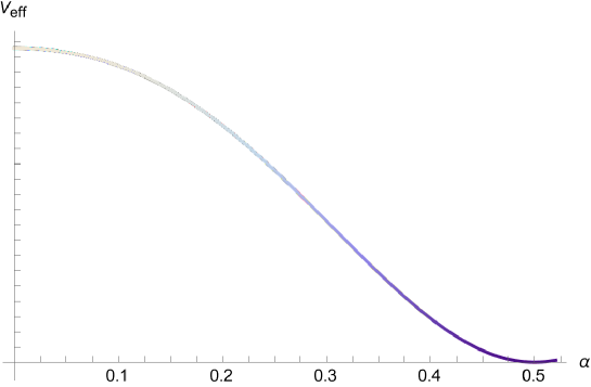
Figure 1: Effective potential of Sp(6) gauge fields $V^{\text{g}}_{\text{eff}}$. The potential minimum is found to be $\alpha_{\text{min}}=\frac{1}{2}$.

4.2 Fermions

In this subsection, we discuss possibilities that a realistic Higgs mass as well as the electroweak symmetry breaking are realized by introducing fermions.

We would like to comment on the SM fermions in our model before the Higgs potential analysis. In the $Sp(6)$ model, the Higgs doublet is embedded in the $SU(3)$ sextet after the decomposition of $Sp(6)$ representation in order to predict a realistic weak mixing angle. In this case, the electromagnetic charges of the $SU(3)$ triplet is known as $(0,-1,1)^{T}~{}(T:$ Transpose) [10] where the first two components correspond to $SU(2)_{L}$ doublet. On the other hand, the $SU(2)_{L}$ singlet is possible to be embedded into the 2-rank anti-symmetric representation of $SU(3)$ in $Sp(6)$. Since the electromagnetic charges of $SU(3)$ triplet are integers, any fractional charges cannot be obtained by its tensor product. Therefore, the SM quarks are introduced by hand on the 4D brane at the fixed points. In our setup, Yukawa coupling cannot be obtain from the 5D gauge coupling. The SM leptons also have to put on the 4D brane at the fixed points. Yukawa coupling can be obtain by introducing additional massive 5D fermions and coupling them to the SM fermions through the Dirac mass terms [5]. In any case, the SM fermions and additional fermions to realize Yukawa couplings are massive. Note that the contribution of the one-loop effective potential of the massive fermion is strongly suppressed by the Boltzman-like factor $e^{-\pi MR}$, where $M$ is the 5D fermion mass. Since the effects for the electroweak symmetry breaking by such type of the potential is known to be negligible, we do not consider them hereafter in this paper.

First, we consider the case of introducing fermions in the adjoint representation. Since the differences are the degrees of freedom and an overall sign in the potential between the adjoint representation fermions and the gauge fields, the effective potential is totally given by

$$V_{\text{eff}}^{\text{1-loop}} =V^{g}_{\text{eff}}+V^{f_{\text{ad}}}_{\text{eff}}$$

$$=\frac{3(4N_{\text{ad}}-3)}{64\pi^{6}R^{4}}\sum_{k=1}^{\infty}\frac{1}{k^{5}}\quantity[\{1+2(-1)^{k}\}\cos(2\pi k\alpha)+2\{1+(-1)^{k}\}\cos(\pi k\alpha)],$$ (4.10)

where $N_{\text{ad}}$ is the number of the adjoint representation fermion. The sign of the curvature of the potential at $\alpha_{\text{min}}$ depends on the value of $N_{\text{ad}}$ as follows.

$$(N_{\text{ad}}=0)\qquad \evaluated{\partialderivative{{}^{2}}{{\alpha}^{2}}V_{\text{eff}}^{\text{1-loop}}}_{\alpha=0}<0,\quad\evaluated{\partialderivative{{}^{2}}{{\alpha}^{2}}V_{\text{eff}}^{\text{1-loop}}}_{\alpha=\frac{1}{2}}>0$$ (4.11)

$$(N_{\text{ad}}>0),\qquad \evaluated{\partialderivative{{}^{2}}{{\alpha}^{2}}V_{\text{eff}}^{\text{1-loop}}}_{\alpha=0}>0,\quad\evaluated{\partialderivative{{}^{2}}{{\alpha}^{2}}V_{\text{eff}}^{\text{1-loop}}}_{\alpha=\frac{1}{2}}<0.$$ (4.12)

Therefore, the electroweak symmetry cannot be broken when only adjoint representation fermions are introduced.

Next, we consider fermions in a $Sp(6)$ fundamental representation and its KK mass spectrum. From the $Z_{2}$ invariance of $\mathcal{L}_{5}$, the boundary conditions of 5D fermion in the representation $R$ at the fixed points are

$$\Psi(x^{\mu},x^{5}_{i}-x^{5})=R(P_{i})(-i\Gamma^{5})\Psi(x^{\mu},x^{5}_{i}+x^{5}).$$ (4.13)

The $Z_{2}$ parity of each component in the $Sp(6)$ sextet is given as

$$\Psi=\begin{pmatrix}\matrixquantity{\psi_{1}^{(++)}\\[2.84526pt] \psi_{2L}^{(++)}\\[2.84526pt] \psi_{3}^{(-+)}\\ \hline\cr\psi_{4}^{(+-)}\\[2.84526pt] \psi_{5}^{(+-)}\\[2.84526pt] \psi_{6}^{(--)}}\end{pmatrix}.$$ (4.14)

The $Sp(6)$ sextet can be decomposed into the $SU(3)$ representation: $\bf{6}\rightarrow 3+\overline{3}$ and furthermore into the $SU(2)$ representation through $\bf{3}\rightarrow\bf{2}+\bf{1}$.

$$\bf{6} \xRightarrow{SU(3)}\ {\bf{3}+\overline{\bf{3}}}\ \xRightarrow{SU(2)}\ {\bf{2}}_{(++)}+\bf{1}_{(-+)}+{\bf{2}}_{(+-)}+\bf{1}_{(--)}.$$ (4.15)

From the above information of decomposition, the KK mass spectrum of $Sp(6)$ sextet can be read as follows. For the $SU(2)$ doublet, the KK index receives a constant shift as $n\to n+\frac{\alpha}{2}$. Taking into account $Z_{2}$ parity, the KK spectrum of the $Sp(6)$ sextet can be found,

$$M_{n}^{2}=\left(\frac{n+\frac{\alpha}{2}}{R}\right)^{2},\;\left(\frac{n+\frac{1}{2}}{R}\right)^{2},\;\left(\frac{(n+\frac{1}{2})+\frac{\alpha}{2}}{R}\right)^{2},\;\left(\;\frac{n}{R}\;\right)^{2}.$$ (4.16)

Since the KK mass spectrum of the $SU(2)$ singlet component is independent of the Higgs VEV parameter $\alpha$, the contribution to the potential can be neglected in our analysis of electroweak symmetry breaking. This argument can be easily extended to a $N$-rank totally symmetric representation of $SU(2)$ doublets. In this case, we need to know the covariant derivative of the $SU(2)$ $N$-rank totally symmetric representation, which is given by

$$D_{5}\Psi_{i_{1}\cdots i_{N}}=(\delta_{i_{1}i_{1}^{\prime}}\partial_{5}+NigA_{5}^{a}T^{a}_{i_{1}i_{1}^{\prime}})\Psi_{i_{1}^{\prime}\cdots i_{N}}.$$ (4.17)

where an additional factor $N$ appears from the symmetric indices $i_{1},\cdots,i_{N}$. This allows us to know the KK mass spectrum of the general $N$-rank totally symmetric representation fermions. The $SU(2)$ $N$-rank totally symmetric representation is [${\bf{N+1}}$] dimensional representation of $SU(2)$. The KK mass spectrum of the [${\bf{N+1}}$] dimensional representation with $Z_{2}$ parity $(++)$ is obtained below,

$$(N=\text{odd})\qquad M^{2}_{n}=\left(\frac{n+\frac{N\alpha}{2}}{R}\right)^{2},\ \left(\frac{n+\frac{(N-2)\alpha}{2}}{R}\right)^{2},\cdots,\left(\frac{n+\frac{\alpha}{2}}{R}\right)^{2},$$ (4.18)

$$(N=\text{even})\qquad M^{2}_{n}=\left(\frac{n+\frac{N\alpha}{2}}{R}\right)^{2},\ \left(\frac{n+\frac{(N-2)\alpha}{2}}{R}\right)^{2},\cdots,\left(\frac{n+\alpha}{R}\right)^{2}.$$ (4.19)

As will be seen below, the realistic electroweak symmetry breaking is possible in the $N=4$ case. The 4-rank totally symmetric representation of $Sp(6)$ is ${\bf{126}}$ dimensional representation, which can be decomposed into the $SU(3)$ representation as follows.

$${\bf{126}}\quad\xRightarrow{SU(3)}\quad{\bf{27}}+\bf{24}+\bf{24}+{\bf{15}}+\overline{\bf{15}}+\bf{8}+\bf{6}+\overline{\bf{6}}+\bf{1}$$ (4.20)

Each $SU(3)$ representation is further decomposed into $SU(2)$ representation with the corresponding $Z_{2}$ parity as follows.

$${\bf{27}} \xRightarrow{SU(2)}{\bf{5}}_{(++)}\ +\ {\bf{4}}_{(-+)}\times 2\ +\ {\bf{3}}_{(++)}\times 3\ +\ {\bf{2}}_{(-+)}\times 2\ +\ {\bf{1}}_{(++)},$$

$$\bf{24} \xRightarrow{SU(2)}{\bf{5}}_{(+-)}\ +\ {\bf{4}}_{(--)}\times 2\ +\ {\bf{3}}_{(+-)}\times 2\ +\ {\bf{2}}_{(--)}\times 2\ +\ {\bf{1}}_{(+-)},$$

$$\bf{15},\overline{\bf{15}} \xRightarrow{SU(2)}{\bf{5}}_{(++)}\ +\ {\bf{4}}_{(-+)}\ +\ {\bf{3}}_{(++)}\ +\ {\bf{2}}_{(-+)}\ +\ {\bf{1}}_{(++)},$$

$$\bf{8} \xRightarrow{SU(2)}{\bf{3}}_{(+-)}\ +\ {\bf{2}}_{(--)}\times 2\ +\ {\bf{1}}_{(+-)},$$

$$\bf{6},\overline{\bf{6}} \xRightarrow{SU(2)}{\bf{3}}_{(++)}\ +\ {\bf{2}}_{(-+)}\ +\ {\bf{1}}_{(++)}.$$ (4.21)

These decomposition can be easier to obtain by using Young tableau as shown in Appendix B. Then, we obtain the effective potential of 4-rank totally symmetric representation of $Sp(6)$ as follows.

$$V_{\text{eff}}^{f_{4}} =\frac{3}{16\pi^{6}R^{4}}\sum_{k=1}^{\infty}\frac{1}{k^{5}}[\{3+2(-1)^{k}\}\cos(4\pi k\alpha)+\{4+4(-1)^{k}\}\cos(3\pi k\alpha)$$

$$\hskip 85.0pt+\{10+7(-1)^{k}\}\cos(2\pi k\alpha)+\{10+10(-1)^{k}\}\cos(\pi k\alpha)].$$ (4.22)

We analyze the effective potential from the gauge field and a fermion in the 4-rank totally symmetric representation $V_{\text{eff}}^{\text{1-loop}}=V_{\text{eff}}^{g}+V_{\text{eff}}^{f_{4}}$. It has a negative curvature at $\alpha=0,\ \frac{1}{2}$:

$$\evaluated{\partialderivative{{}^{2}}{{\alpha}^{2}}V_{\text{eff}}^{\text{1-loop}}}_{\alpha=0}= -\frac{75}{8\pi^{4}R^{4}}\zeta(3)\quad<0,$$

$$\evaluated{\partialderivative{{}^{2}}{{\alpha}^{2}}V_{\text{eff}}^{\text{1-loop}}}_{\alpha=\frac{1}{2}}= -\frac{951}{512\pi^{4}R^{4}}\zeta(3)<0.$$ (4.23)

The minimum is located in a range of $0<\alpha_{\text{min}}<1/2$ and the Figure 2 shows $\alpha_{\text{min}}\simeq 0.4069$. Therefore, the contribution from the 4-rank totally symmetric representation can realize the realistic electroweak symmetry breaking.

$$Sp(6)\xrightarrow{Z_{2}\>\text{orbifold}}SU(2)_{L}\times U(1)_{Y}\times U(1)_{X}\xrightarrow{\text{quantum effect}}U(1)_{em}\times U^{\prime}(1)$$

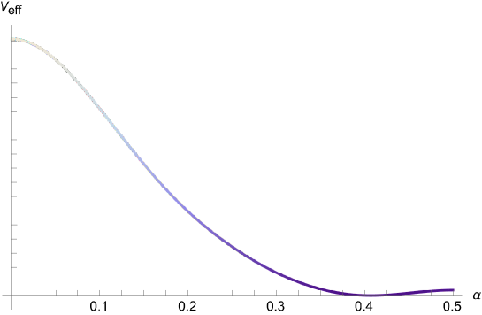
Figure 2: Effective potential of the gauge field and a 4-rank totally symmetric representation $V^{g}_{\text{eff}}+V^{\text{$f_{4}$}}_{\text{eff}}$.  The potential minimum is found to be $\alpha_{\text{min}}\simeq 0.4069.$

5 Higgs mass

In GHU, Higgs mass is likely to be small since Higgs potential is generated by quantum corrections. Obtaining the realistic Higgs mass is therefore very nontrivial in GHU. We note that the 4D gauge coupling constant and the compactification scale are related to the W-boson mass as

$$m_{W}^{2}=\frac{(g_{4}v)^{2}}{8}=\frac{{\alpha^{2}_{\text{min}}}}{4R^{2}}=(80.4\ \text{GeV})^{2}.$$ (5.1)

When the 4-rank totally symmetric representation is introduced, the minimum is located at $\alpha_{\text{min}}\sim\mathcal{O}(0.1)$, which implies that the compactification scale is $\mathcal{O}(100)\ \text{GeV}$. To improve this result, the minimum should be smaller, $\alpha_{\text{min}}\sim\mathcal{O}(0.01)$. Then, the compactification scale would be the order of $\mathcal{O}(10)$ TeV, and the Higgs mass would be predicted to be $\mathcal{O}(100)$ GeV. In order to realize such a situation, we notice that the potential by fermions in the adjoint representation takes an upside-down form of the potential from the gauge field shown in Figure 1. From the property that the potential by the fermions in the adjoint representation takes the minimum at the origin, the effects of the potential is expected for the minimum to get closer to the origin. Therefore, we consider introducing fermions in both the 4-rank totally symmetric representation and the adjoint representation: $V_{\text{eff}}^{\text{1-loop}}=V_{\text{eff}}^{g}+V_{\text{eff}}^{f_{4}}+N_{\text{ad}}V_{\text{eff}}^{f_{\text{ad}}}$. To occur the electroweak symmetry breaking, the curvature of the potential at $\alpha=0,\ \frac{1}{2}$ must be negative as discussed in the previous section. The curvature at $\alpha=\frac{1}{2}$ is negative for arbitrary $N_{\text{ad}}$, and the curvature at $\alpha=0$ is negative if the number of adjoint representation fermions satisfies the condition below.

$$\evaluated{\partialderivative{{}^{2}}{{\alpha}^{2}}V_{\text{eff}}^{\text{1-loop}}}_{\alpha=0}= \frac{36N_{\text{ad}}-1335}{128\pi^{4}R^{4}}\zeta(3)\ <0,\quad\therefore\ N_{\text{ad}}<38.$$ (5.2)

Hereafter, we consider the case $N_{\text{ad}}<38$. Now, we study whether a realistic Higgs mass can be obtained in our model. The $N_{\text{ad}}$ dependence on the Higgs mass in Figure 4 shows that $m_{h}\simeq 123.5\ \text{[GeV]}$ is realized at $N_{\text{ad}}=31$. Calculating the potential in the case of $N_{\text{ad}}=31$, we can see that the minimum is $\alpha_{\text{min}}\simeq 0.0424$ from Figure 4. This gives a compactification scale to be $\frac{1}{R}\simeq 3.796\ [\text{TeV}]$.

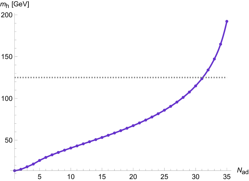
Figure 3: SM Higgs mass $m_{h}$ as a function of the number of the adjoint fermions.

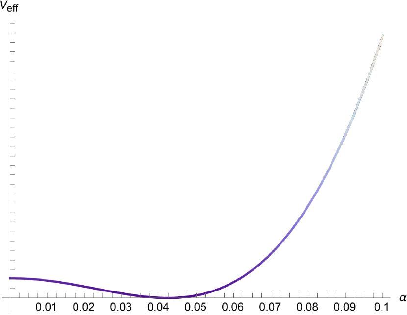
Figure 4: Effective potential $V_{\text{eff}}^{g}+V_{\text{eff}}^{f_{4}}+N_{\text{ad}}V_{\text{eff}}^{f_{\text{ad}}}$ in the case of $N_{\text{ad}}=31$.  The potential minimum is $\alpha_{\text{min}}\simeq 0.0424.$

6 Conclusion

In this paper, we have studied the electroweak symmetry breaking and Higgs mass in a five dimensional $Sp(6)$ gauge-Higgs unification model. One of the advantages to consider this model is that the weak mixing angle is predicted to be $\sin^{2}\theta_{W}=1/4$ at the compactification scale [10]. In GHU, the non-local Higgs potential is generated at one-loop level although the Higgs potential at tree level is vanished by the gauge invariance. Therefore, Higgs mass is likely to be small and obtaining a realistic Higgs mass is a very non-trivial problem in GHU. In our analysis, it is shown that the realistic electroweak symmetry breaking and Higgs mass can be realized by introducing additional fermions in a 4-rank totally symmetric representation and thirty one adjoint representations.

Although we have obtained a realistic pattern of the electroweak symmetry breaking and Higgs mass, the compactification scale is somewhat small and the number of adjoint fermion is relatively large. To improve these points, one of the approach is to utilize the gauge kinetic terms localized at the fixed points[5]. Their effects is known to enhance the magnitude of the compactification scale, which makes a viable Higgs mass easier and expects to help the number of additional fermions ruduced. This issue is left for our future work.

Acknowledgments

This work was supported by JST SPRING, Grant Number JPMJSP2139 (A.N.).

Appendix A $Sp(6)$ generators

The $Sp(6)$ generators $T^{a}\ (a=1,\cdots,21)$ are given by $T^{a}=\frac{1}{2\sqrt{2}}t^{a}$ with the following $t^{a}$.

$$t^{a} =\begin{pmatrix}\matrixquantity{\lambda^{a}&0\\ 0&-(\lambda^{a})^{*}}\end{pmatrix}\qquad(a=1,\cdots 8),$$ (A.1)

$$t^{9} =\sqrt{\frac{2}{3}}\begin{pmatrix}\matrixquantity{I&0\\ 0&-I}\end{pmatrix},$$ (A.2)

$$t^{a} =\begin{pmatrix}\matrixquantity{0&M_{j}\\ M_{j}&0}\end{pmatrix}\qquad(a=9+j,\;j=1\cdots 6),$$ (A.3)

$$t^{a} =\begin{pmatrix}\matrixquantity{0&-iM_{j}\\ iM_{j}&0}\end{pmatrix}\qquad(a=15+j,\;j=1\cdots 6),$$ (A.4)

where $\lambda^{a}$ is a Gelman matrix and $M_{j}$ is

$$M_{1} =\begin{pmatrix}\matrixquantity{\sqrt{2}&0&0\\ 0&0&0\\ 0&0&0}\end{pmatrix},\;M_{2}=\begin{pmatrix}\matrixquantity{0&0&0\\ 0&\sqrt{2}&0\\ 0&0&0}\end{pmatrix},\;M_{3}=\begin{pmatrix}\matrixquantity{0&0&0\\ 0&0&0\\ 0&0&\sqrt{2}}\end{pmatrix},$$

$$M_{4} =\begin{pmatrix}\matrixquantity{0&1&0\\ 1&0&0\\ 0&0&0}\end{pmatrix},\;M_{5}=\begin{pmatrix}\matrixquantity{0&0&0\\ 0&0&1\\ 0&1&0}\end{pmatrix},\;M_{6}=\begin{pmatrix}\matrixquantity{0&0&1\\ 0&0&0\\ 1&0&0}\end{pmatrix}.$$ (A.5)

These $T^{a}$ are normalized as $\Tr(T^{a}T^{b})=\frac{1}{2}\delta^{ab}$.

Appendix B Decomposition of 4-rank totally symmetric representation

In this appendix B, we summarize the decomposition of the 4-rank totally symmetric representation of $Sp(6)$ into $SU(2)$ irreducible representations by using Young tablaeu.

First, the decomposition of $Sp(6)$ sextet into $SU(2)$ irreducible representations ${\bf{6}}\xRightarrow{SU(3)}{\bf{3}}+\overline{\bf{3}}\xRightarrow{SU(2)}{\bf{2}}+{\bf{1}}+\overline{\bf{2}}+{\bf{1}}$ is shown.

(B.7)

(B.9)

Here,the

2$and$¯2$representationareessentiallythesame,butthe$2$obtainedbydecomposingthe$3$andthe$¯2$obtainedbydecomposingthe$¯3$aredifferentinparitysignInordertodistinguishbetweenthem,$¯2$ismarkedwithacoloredbox.Hereafter$⊗$meanssymmetricproduct.\par Next,welookatthedecompositionofthe4-ranktotallyrepresentationof$Sp(6)$.\begin{aligned} \ytableausetup{mathmode,boxsize=2em}&\ydiagram[]{4}\\[19.91692pt] &\xRightarrow{SU(3)}\left(\;\ydiagram[*(lime)]{2,2}+\ydiagram[*(lime)]{1,1}*[*(white)]{1+1}+\ydiagram[]{2}+{\bf{1}}\;\right)\otimes\left(\;\ydiagram[*(lime)]{2,2}+\ydiagram[*(lime)]{1,1}*[*(white)]{1+1}+\ydiagram[]{2}+{\bf{1}}\;\right)\\[19.91692pt] &\quad=\quad\ydiagram[*(lime)]{2,2}*[*(white)]{2+2}+\ydiagram[*(lime)]{1,1}*[*(white)]{1+3}+\ydiagram[*(lime)]{3,3}*[*(white)]{3+1}\\ &\qquad+\quad\ydiagram[*(lime)]{4,4}+\ydiagram[]{4}+\ydiagram[*(lime)]{1,1}*[*(white)]{1+1}+\ydiagram[*(lime)]{2,2}+\ydiagram[]{2}+{\bf{1}}\end{aligned}Therefore,weobtainthedecompositionthe4-ranktotallyrepresentationof$Sp(6)$into$SU(3)$irreduciblerepresentation:\begin{equation}\bf{126}\quad=\quad{\bf{27}}+\bf{24}+\bf{24}+\overline{\bf{15}}+\bf{15}+\bf{8}+\bf{6}+\overline{\bf{6}}+\bf{1}.\end{equation}Then,thedecompositionsofeachmultipletinto$SU(2)$irreduciblerepresentaitonsarelisted.\par\noindent(i)\ {\bf{27}}rep.\begin{aligned} &\ydiagram[*(lime)]{2,2}*[*(white)]{2+2}\\[14.22636pt] &\xRightarrow{SU(2)}\left(\;\ydiagram[*(lime)]{2}_{(++)}+\ydiagram[*(lime)]{1}_{(-+)}+{\bf{1}}_{(++)}\;\right)\otimes\left(\;\ydiagram[]{2}_{(++)}+\ydiagram[]{1}_{(-+)}+{\bf{1}}_{(++)}\;\right)\\[19.91692pt] &\quad=\quad\ydiagram[*(lime)]{2}*[*(white)]{2+2}_{(++)}+\ydiagram[*(lime)]{1}*[*(white)]{1+2}_{(-+)}+\ydiagram[]{2}_{(++)}\\ &\quad\quad+\ydiagram[*(lime)]{2}*[*(white)]{2+1}_{(-+)}+\ydiagram[*(lime)]{1}*[*(white)]{1+1}_{(++)}+\ydiagram[]{1}_{(-+)}\\ &\quad\quad+\ydiagram[*(lime)]{2}_{(++)}+\ydiagram[*(lime)]{1}_{(-+)}+{\bf{1}}_{(++)}\end{aligned}(ii)\ {\bf{24}}rep.\begin{aligned} &\ydiagram[*(lime)]{1,1}*[*(white)]{1+3}\\[14.22636pt] &\xRightarrow{SU(2)}\left(\;\ydiagram[*(lime)]{1}*[*(white)]{1+1}_{(+-)}+\ydiagram[]{1}_{(--)}+\ydiagram[*(lime)]{1}_{(--)}+{\bf{1}}_{(+-)}\;\right)\\[5.69054pt] &\hskip 250.0pt\otimes\left(\;\ydiagram[]{2}_{(++)}+\ydiagram[]{1}_{(-+)}+{\bf{1}}_{(++)}\;\right)\\[14.22636pt] &\quad=\quad\ydiagram[*(lime)]{1}*[*(white)]{1+3}_{(+-)}+\ydiagram[]{3}_{(--)}+\ydiagram[*(lime)]{1}*[*(white)]{1+2}_{(--)}+\ydiagram[]{2}_{(+-)}\\ &\quad\quad+\ydiagram[*(lime)]{1}*[*(white)]{1+1}_{(+-)}+\ydiagram[]{1}_{(--)}\\ &\quad\quad+\ydiagram[*(lime)]{1}_{(--)}+{\bf{1}}_{(+-)}\end{aligned}(iii)\ {\bf{24}}rep.\begin{aligned} &\ydiagram[*(lime)]{3,3}*[*(white)]{3+1}\\[14.22636pt] &\xRightarrow{SU(2)}\left(\;\ydiagram[*(lime)]{2}_{(++)}+\ydiagram[*(lime)]{1}_{(-+)}+{\bf{1}}_{(++)}\;\right)\otimes\left(\;\ydiagram[*(lime)]{1}*[*(white)]{1+1}_{(+-)}+\ydiagram[]{1}_{(--)}+\ydiagram[*(lime)]{1}_{(--)}+{\bf{1}}_{(+-)}\;\right)\\[14.22636pt] &\quad=\quad\ydiagram[*(lime)]{3}*[*(white)]{3+1}_{(+-)}+\ydiagram[*(lime)]{2}*[*(white)]{2+1}_{(--)}+\ydiagram[*(lime)]{1}*[*(white)]{1+1}_{(+-)}\\ &\quad\quad+\ydiagram[]{1}_{(--)}\\ &\quad\quad+\ydiagram[*(lime)]{3}_{(--)}+\ydiagram[*(lime)]{2}_{(+-)}+\ydiagram[*(lime)]{1}_{(--)}\\ &\quad\quad+{\bf{1}}_{(+-)}\\ \end{aligned}(iv)\ {\bf{15}}rep.\begin{aligned} &\ydiagram[]{4}\\[14.22636pt] &\xRightarrow{SU(2)}\left(\;\ydiagram[]{2}_{(++)}+\ydiagram[]{1}_{(-+)}+{\bf{1}}_{(++)}\;\right)\otimes\left(\;\ydiagram[]{2}_{(++)}+\ydiagram[]{1}_{(-+)}+{\bf{1}}_{(++)}\;\right)\\[19.91692pt] &\quad=\quad\ydiagram[]{4}_{(++)}+\ydiagram[]{3}_{(-+)}+\ydiagram[]{2}_{(++)}\\ &\quad\quad+\ydiagram[]{1}_{(-+)}\\ &\quad\quad+{\bf{1}}_{(++)}\end{aligned}(v)\$¯15$rep.\begin{aligned} &\ydiagram[*(lime)]{4,4}\\[14.22636pt] &\xRightarrow{SU(2)}\left(\;\ydiagram[*(lime)]{2}_{(++)}+\ydiagram[*(lime)]{1}_{(-+)}+{\bf{1}}_{(++)}\;\right)\otimes\left(\;\ydiagram[*(lime)]{2}_{(++)}+\ydiagram[*(lime)]{1}_{(-+)}+{\bf{1}}_{(++)}\;\right)\\[14.22636pt] &\quad=\quad\ydiagram[*(lime)]{4}_{(++)}+\ydiagram[*(lime)]{3}_{(-+)}+\ydiagram[*(lime)]{2}_{(++)}\\ &\quad\quad+\ydiagram[*(lime)]{1}_{(-+)}\\ &\quad\quad+{\bf{1}}_{(++)}\end{aligned}(vi)\ {\bf{8}}rep.\begin{aligned} \ydiagram[*(lime)]{1,1}*[*(white)]{1+1}&\xRightarrow{SU(2)}\left(\;\ydiagram[*(lime)]{1}*[*(white)]{1+1}_{(+-)}+\ydiagram[]{1}_{(--)}+\ydiagram[*(lime)]{1}_{(--)}+{\bf{1}}_{(+-)}\;\right)\otimes{\bf{1}}_{(++)}\\[14.22636pt] &\quad=\quad\ydiagram[*(lime)]{1}*[*(white)]{1+1}_{(+-)}+\ydiagram[]{1}_{(--)}+\ydiagram[*(lime)]{1}_{(--)}+{\bf{1}}_{(+-)}\end{aligned}(vii)\ {\bf{6}}rep.\begin{aligned} \ydiagram[]{2}&\xRightarrow{SU(2)}\left(\;\ydiagram[]{2}_{(++)}+\ydiagram[]{1}_{(-+)}+{\bf{1}}_{(++)}\;\right)\otimes{\bf{1}}_{(++)}\\[14.22636pt] &\quad=\quad\ydiagram[]{2}_{(++)}+\ydiagram[]{1}_{(-+)}+{\bf{1}}_{(++)}\end{aligned}(viii)\$¯6$rep.\begin{aligned} \ydiagram[*(lime)]{2,2}&\xRightarrow{SU(2)}\left(\;\ydiagram[*(lime)]{2}_{(++)}+\ydiagram[*(lime)]{1}_{(-+)}+{\bf{1}}_{(++)}\;\right)\otimes{\bf{1}}_{(++)}\\[14.22636pt] &\quad=\quad\ydiagram[*(lime)]{2}_{(++)}+\ydiagram[*(lime)]{1}_{(-+)}+{\bf{1}}_{(++)}\end{aligned}Insummary,each$SU(3)$representationsfromthe4-ranktotallysymmetricrepresentationof$Sp(6)$aredecomposedinto$SU(2)$representationsbelow.\begin{aligned} {\bf{27}}&\xRightarrow{SU(2)}{\bf{5}}_{(++)}\ +\ {\bf{4}}_{(-+)}\times 2\ +\ {\bf{3}}_{(++)}\times 3\ +\ {\bf{2}}_{(-+)}\times 2\ +\ {\bf{1}}_{(++)},\\ \bf{24}&\xRightarrow{SU(2)}{\bf{5}}_{(+-)}\ +\ {\bf{4}}_{(--)}\times 2\ +\ {\bf{3}}_{(+-)}\times 2\ +\ {\bf{2}}_{(--)}\times 2\ +\ {\bf{1}}_{(+-)},\\ \bf{15},\overline{\bf{15}}&\xRightarrow{SU(2)}{\bf{5}}_{(++)}\ +\ {\bf{4}}_{(-+)}\ +\ {\bf{3}}_{(++)}\ +\ {\bf{2}}_{(-+)}\ +\ {\bf{1}}_{(++)},\\ \bf{8}&\xRightarrow{SU(2)}{\bf{3}}_{(+-)}\ +\ {\bf{2}}_{(--)}\times 2\ +\ {\bf{1}}_{(+-)}\\ \bf{6},\overline{\bf{6}}&\xRightarrow{SU(2)}{\bf{3}}_{(++)}\ +\ {\bf{2}}_{(-+)}\ +\ {\bf{1}}_{(++)}.\end{aligned}\par\par\par\thebibliography\lx@bibitem{Fairlie}D.~{}B.~{}Fairlie,``Higgs^{\prime}FieldsAndTheDeterminationOfTheWeinbergAngle,^{\prime\prime}Phys.\ Lett.\ B{\bf 82},97(1979);``TwoConsistentCalculationsOfTheWeinbergAngle,^{\prime\prime}J.\ Phys.\ G{\bf 5},L55(1979).\par\lx@bibitem{Manton}N.S.Manton,``ANewSix-DimensionalApproachtotheWeinberg-SalamModel,"Nucl.Phys.B158(1979)141-153.\par\lx@bibitem{Hosotani}Y.Hosotani,``DynamicalMassGenerationbyCompactExtraDimension,"Phys.Lett.\textbf{126B}(1983)309;Y.Hostonani,``DynamicalofNon-integrablePhasesandGaugeSymmetryBreaking,"ANNALS\textbf{190},(1989)233-253\par\par\lx@bibitem{HIL}H.~{}Hatanaka,T.~{}InamiandC.S.~{}Lim,``TheGaugehierarchyproblemandhigherdimensionalgaugetheories,^{\prime\prime}Mod.\ Phys.\ Lett.\ A{\bf 13},2601(1998);[hep-th/9805067].\par\lx@bibitem{SSS}C.~{}A.~{}Scrucca,M.~{}SeroneandL.~{}Silvestrini,``Electroweaksymmetrybreakingandfermionmassesfromextradimensions,^{\prime\prime}Nucl.Phys.B\textbf{669},128-158(2003),[arXiv:hep-ph/0304220[hep-ph]].\par\lx@bibitem{ABQ}I.~{}Antoniadis,K.~{}BenakliandM.~{}Quiros,``FiniteHiggsmasswithoutsupersymmetry,^{\prime\prime}NewJ.\ Phys.\ {\bf 3},20(2001);[arXiv:hep-th/0108005].\par\par\lx@bibitem{MY}N.~{}MaruandT.~{}Yamashita,``Two-loopcalculationofHiggsmassingauge-Higgsunification:5DmasslessQEDcompactifiedonS**1,^{\prime\prime}Nucl.\ Phys.\ B{\bf 754},127(2006);[arXiv:hep-ph/0603237].\par\lx@bibitem{HMTY}Y.~{}Hosotani,N.~{}Maru,K.~{}TakenagaandT.~{}Yamashita,``TwoloopfinitenessofHiggsmassandpotentialinthegauge-Higgsunification,^{\prime\prime}Prog.\ Theor.\ Phys.\ {\bf 118},1053(2007);[arXiv:0709.2844[hep-ph]].\par\lx@bibitem{LMH}C.S.~{}Lim,N.~{}MaruandK.~{}Hasegawa,``Sixdimensionalgauge-HiggsunificationwithanextraspaceS**2andthehierarchyproblem,^{\prime\prime}J.\ Phys.\ Soc.\ Jap.\ {\bf 77},074101(2008);arXiv:hep-th/0605180.\par\lx@bibitem{HLM}K.~{}Hasegawa,C.~{}S.~{}LimandN.~{}Maru,``PredictionsoftheHiggsmassandtheweakmixingangleinthe6Dgauge-Higgsunification,^{\prime\prime}J.Phys.Soc.Jap.\textbf{85},no.7,074101(2016);[arXiv:1509.04818[hep-ph]].\par\par\lx@bibitem{CGM}C.~{}Csaki,C.~{}GrojeanandH.~{}Murayama,``StandardmodelHiggsfromhigherdimensionalgaugefields,^{\prime\prime}Phys.Rev.D\textbf{67}(2003),085012[arXiv:hep-ph/0210133[hep-ph]].\par\par\par\endthebibliography\par\par\par\par\par\par\par\par\par$