[en-GB]showdayofmonth=false
Temporal Wasserstein Imputation: Versatile Missing Data Imputation for Time Series
Abstract
Missing data often significantly hamper standard time series analysis, yet in practice they are frequently encountered. In this paper, we introduce temporal Wasserstein imputation, a novel method for imputing missing data in time series. Unlike existing techniques, our approach is fully nonparametric, circumventing the need for model specification prior to imputation, making it suitable for potential nonlinear dynamics. Its principled algorithmic implementation can seamlessly handle univariate or multivariate time series with any missing pattern. In addition, the plausible range and side information of the missing entries (such as box constraints) can easily be incorporated. As a key advantage, our method mitigates the distributional bias typical of many existing approaches, ensuring more reliable downstream statistical analysis using the imputed series. Leveraging the benign landscape of the optimization formulation, we establish the convergence of an alternating minimization algorithm to critical points. Furthermore, we provide conditions under which the marginal distributions of the underlying time series can be identified. Our numerical experiments, including extensive simulations covering linear and nonlinear time series models and an application to a real-world groundwater dataset laden with missing data, corroborate the practical usefulness of the proposed method.
Keywords— Missing data, Optimal transport, Nonlinear time series, Threshold AR model, Compositional time series, Nonstationary time series
1 Introduction
In many scientific fields, data collection technology is often subject to various disruptions such as idiosyncratic or system-level instrument failures or changes in data-collection policies, leading to missing entries in the data (Little and Rubin,, 2019). In time series analysis, missing data pose serious challenges to the application of most statistical tools since it is typically presumed that observations are available at equally spaced time points. Moreover, since the dynamic relationship is of crucial importance in time series analysis, one can not proceed by throwing away the missing data, even if the missing data appear completely at random (i.e., the missing pattern is independent of the series).
To tackle this issue, one approach is to impute the missing entries, after which the vast array of time series methods can be readily applied for statistical inference in the downstream. Naturally, the estimation of the optimal interpolator, which is the expectation of the missing data conditional on the observed data, has been extensively studied (Harvey and Pierse,, 1984; Pourahmadi,, 1989; Peña and Maravall,, 1991; Gómez et al.,, 1999; Alonso and Sipols,, 2008; Peña and Tsay,, 2021). Most of these methods are iterative or EM-type algorithms that alternate between model identification and missing data imputation (see, for example, Chpt. 4 of Peña and Tsay,, 2021). For certain time series models, one can estimate the model parameters simultaneously with the missing data (Harvey and Pierse,, 1984; Gómez et al.,, 1999). Besides the optimal interpolator, ad hoc deterministic imputation methods, such as smoothing with linear interpolation, B-splines and wavelets (see, for instance, Hastie et al.,, 2009), are also used in practice for their simplicity.
However, the optimal interpolator can introduce distributional biases that are detrimental to downstream statistical analysis. To illustrate, consider an AR(1) model, , where and is a sequence of i.i.d. standard normal random variables. It is well-known that the optimal interpolator can be expressed in terms of the inverse autocorrelation function (Peña and Maravall, 1991; see also Chpt. 6 of Peña et al.,, 2011). For instance, suppose that data at time and are missing; then the optimal interpolators are given by
Using the fact that for , it is not difficult to show
and
Hence, the variance and the autocovariances of the imputed data are different from those of the original AR(1) process. Intuitively, the optimal interpolator for consecutive missing data tends to predict the unconditional mean, leading to a downward bias (in magnitude) of the variances. In general, the joint distribution of the optimally interpolated time series is often quite different from that of the original process, leading to questionable downstream statistical analysis, especially when the number of missing data is non-negligible. Similar biases are also observed for some deterministic imputation methods (Carrizosa et al.,, 2013).
In addition to the distributional bias, the above example also reveals further predicaments of the optimal interpolator. First, in order to compute the optimal interpolator, one often needs to choose a model class (such as the ARMA models) before imputation. However, such decision relies heavily on domain expertise and may be ill-informed when there are many missing values. Second, it may be difficult to compute the optimal interpolator if some nonlinear model is employed. With different missing patterns and different chosen models, the computational procedure may change drastically. Finally, incorporating side information about the missing data into this methodology appears less straightforward. Side information about the missing data restricts the set of admissible imputations. For instance, compositional time series is known to lie in and sums to unity at each time point. Besides the optimal interpolator, it is well-known that some deterministic interpolators such as B-spline smoothing are also inclined to over-(or under-)shoot, leading to imputations that are outside plausible ranges (Carrizosa et al.,, 2013).
In this paper, we present a novel procedure for time series imputation, referred to as the temporal Wasserstein imputation (TWI), which circumvents the aforementioned limitations. As a nonparametric method, TWI is highly versatile and can be applied to a wide range of time series data. In particular, as a key advantage of TWI, it requires no model class specification prior to imputation, allowing it to perform well even when the underlying time series is nonlinear, such as the threshold autoregressive model (TAR, Tong,, 1983). Formulated as an optimization problem, TWI can be implemented efficiently through an alternating minimization algorithm. This principled algorithmic approach allows for the seamless integration of side information by restricting the admissible imputations, and its extension to multivariate time series is also straightforward. The optimization and statistical underpinnings of TWI are closely related to the optimal transport problem (Villani,, 2008, 2021; Cuturi,, 2013), which is briefly reviewed in Section 2. Section 3 maps out the optimization formulation and introduces the computational scheme in detail.
The core idea of TWI is that by minimizing the Wasserstein distance (over all admissible imputations) between the -dimensional marginal distributions before and after a specified time point, the marginal distributions implied by the imputation shall resemble those of the original series (which is stable under stationarity), thereby lowering the distributional bias discussed above. In Section 4, we investigate the optimization and statistical properties of TWI. Our analysis shows that the optimization landscape of TWI is biconvex and the alternating algorithm is guaranteed to converge to a critical point. However, from the statistical viewpoint, missing data imputation suffers from an identification issue: Many distributions (of the stochastic process) may be equally plausible in describing the corrupted series. This raises the question of when and under what conditions TWI can identify the underlying distribution and yield imputations that can be safely used in downstream analysis. In Section 4, we show, via a two-state Markov chain example, that the correct underlying distributions can indeed be identified by TWI under assumptions on the missing pattern and the stability of the imputation. The latter condition motivates a simple modification of TWI, termed -TWI, which shows further improvement in imputation quality from TWI in our numerical experiments.
In Section 5, we evaluate the performance of TWI on synthetic data generated from a wide range of time series models, including nonlinear, multivariate, and nonstationary settings. Across all models, TWI successfully recovers the underlying dynamics and yields favorable downstream statistics such as autocovariance and model parameter estimates. Its advantage is particularly prominent in the presence of nonlinear dynamics, where TWI consistently outperforms the benchmark methods. In Section 6, we apply TWI to a real-world groundwater dataset with many missing data. After imputation, we conduct factor analysis and autoregressive modeling in the downstream. Compared to existing methods, TWI effectively captures the underlying dynamics, producing more reasonable factor estimates as well as more accurate autoregressive predictions. These numerical results underscore the practical utility of TWI.
2 Preliminary: Optimal transport
In this section, we give a brief introduction to the optimal transport (OT) problem, which serves as a prerequisite to the rest of the paper. For a more comprehensive account on the theory of optimal transport, the readers are referred to Villani, (2021, 2008).
Given two probability measures and defined on , and a cost function , the optimal transport cost between and is defined as
where is the set of couplings between and , i.e., probability measures over with marginals and . The classic interpretation for the minimization problem is finding the most cost effective way to move a pile of earth distributed as (with volume normalized to one) to fill a pit whose shape is distributed as . It also has a matching or assignment interpretation that has led to fruitful results in the economics literature (Galichon,, 2016, 2021). If , where is the usual Euclidean distance, and if is absolutely continuous with repsect to the Lebesgue measure, then under some regularity conditions Brenier, (1987) has shown that the optimal coupling which attains the infimum is the push-forward measure, , where is unique -almost everywhere (see also McCann,, 1995). The map , called the optimal transport map, clearly has to satisfy .
If for some , the resulting optimal transport cost is known as the Wasserstein distance of order (to the -th power), which we formally denote as . Namely,
The Wasserstein distance is a metric on the space of probabilities with finite -th moment on , and metrizes the weak topology on this space (Villani,, 2021, Chpt. 9). In particular, if and are probability measures on such that as , then , where denotes the weak convergence of probability measures (Billingsley,, 1995). Therefore, it can be used as a discrepancy metric between and . In fact, the Wasserstein distance offers several advantages over other discrepancy metrics such as the Kullbeck-Leibler divergence or the Kolmogorov-Smirnov distance. In addition to its metric properties, the Wasserstein distance has a nice dual representation and handles support mismatch easily, which makes it suitable in modern machine learning and statistical applications.
If and are discrete measures, for instance and , where are in , , , for all , and denotes the dirac measure at , then the minimization problem becomes the following linear program.
| s.t. | (1) | |||
| (2) | ||||
The constraints (1) and (2) enforce the joint distribution to be a coupling between and , and will henceforth be called the coupling constraints. In the discrete case, the optimal coupling , in general, cannot be expressed as the push-forward under an one-to-one map. Instead, the optimal coupling typically involves split of masses for discrete measures. Many computational methods have been proposed to solve this linear program, including the network flow simplex (Orlin,, 1997) and the auction method (Bertsekas,, 1992). When the problem dimensions are large, standard tools for linear programs may suffer from slow computation. Nevertheless, recent research has made significant progress in the fast computation of the solution through entropic regularization and some algorithms are amenable to large-scale parallelization and can be accelerated with GPUs; see Cuturi, (2013) and Peyré and Cuturi, (2019).
3 Temporal Wasserstein imputation
In this section, we introduce temporal Wasserstein imputation (TWI), the proposed method for time series imputation, through an optimal transport formulation. First, an optimization formulation of the proposed method that directly connects to the optimal transport problem is laid out. Then, we describe an alternating minimization algorithm to impute the missing values. The algorithm also reveals some connections between the proposed method and existing approaches.
3.1 Optimization formulation
Let be the time series of interest, and we observe the time series . Denote by a generic missing value, and the set of time indices corresponding to the missing observations. Then, if and otherwise. If is stationary, it follows that its -dimensional marginal distributions, i.e. the probability distributions of , are stable over time. Let () be the probability measure associated with . Stationarity implies is independent of the time index .
In light of this property, when imputing the missing values in , we seek an imputation whose marginal distributions remain nearly unchanged before and after a specified time point . More specifically, we first divide the time series into two parts and , where , and define the two empirical marginal distributions
The discrepancy between the two empirical distributions can then be measured by the optimal transport cost, which is defined as the minimum value of the following linear program.
| (3) | ||||
where , and, for ease of notation, we enumerate the rows and columns of the matrix by and , respectively. An important special case of (3) is when for some . In this case, we have .
Our goal is to find the imputation that minimizes the aforementioned discrepancy. Thus, we solve for
| (4) |
where the constraint set delineates the admissible imputations. Typically, it enforces the imputation to agree with the observed data, in which case . It may also reflect the side information available. For example, if are weekly sales data, the knowledge of monthly sales define a set of linear constraints for the missing values. Another example is when is a -dimensional compositional time series such as the market share of several companies in an industry. It follows that for all . Then, by defining , where , the set of admissible imputations are restricted to be compositional as well.
One may also consider the following regularized version of (4).
| (5) |
where is small. As we will see in the next subsection, the -regularization term makes a subproblem in the alternating minimization algorithm strongly convex, enhancing numerical stability. In addition, in the important special case corresponding to the Wasserstein distance of order 2, i.e., , the regularization allows one to solve the subproblem by finding a fixed point of a linear system. Since is often chosen to be some power of the Euclidean norm, which induces the Wasserstein distances between the marginal distributions of a time series, the solution to (4) or (5) is called the temporal Wasserstein imputation (TWI) throughout this paper.
In this formulation, it is clear that the temporal Wasserstein imputation, which seeks to equate the marginal distributions on both sides of , is nonparametric. In addition, with a mildly large , the -dimensional marginal distributions can fully capture the nonlinear dynamics of a Markov process (such as a finite-order TAR model), which would otherwise need to be approximated using many parameters in an ARMA model.
3.2 Alternating minimization algorithm
The optimization landscapes of (4) and (5) are complicated because the optimal transport cost is itself the minimum value of a linear program (3), and there are potentially many variables to optimize. This makes directly optimizing (4) or (5) computationally intractable. To remedy this issue, we propose to solve the nested minimization problem using alternating minimization. Since (4) is a special case of (5) with , we focus our discussion on (5).
To begin, observe that with an initialized , problem (3) is exactly the discrete optimal transport problem. The minimizer can be efficiently computed using existing algorithms (Cuturi,, 2013; Peyré and Cuturi,, 2019). Thus, at iteration , treating as fixed, we may compute the optimizer of (3), which corresponds to the inner optimization problem of (5). Next, we optimize (5) over , taking as fixed. This procedure is repeated until convergence. Let
| (6) |
and the procedure described above can be summarized in Algorithm 1. One advantage of the alternating minimization scheme is that the subproblems (steps (a) and (b) in Algorithm 1) are easy to optimize when satisfies some regularity conditions. Optimization guarantees are discussed in the next subsection.
Next, we investigate the properties of Algorithm 1 in an important special case where closed forms can be obtained. Suppose . Then it is not difficult to show that , where
in which all unspecified entries in are zero, and is an matrix of zeros. Hence is quadratic in . In fact, it can be shown that is nonnegative definite for any satisfying the coupling constraints. Moreover, is strongly convex in if (see also Proposition 4 in Section 4). Thus many efficient solvers are applicable in this step (Boyd and Vandenberghe,, 2004; Parikh et al.,, 2014). If, in addition, the constraint set is defined through a system of linear equations, i.e.,
for some known and , then step (b) in Algorithm 1 has the following closed form
| (7) |
where .
Suppose further that . That is, there is no side information about the missing values. In this case, the solution to the subproblem in step (b) must satisfy the following system of linear equations which has the same number of unknowns and equations.
| (8) |
where is treated as fixed. We make a few remarks regarding (8).
Remark 1.
Let us contrast TWI with the optimal interpolator. (8) shows, in general, the temporal Wasserstein imputation is a linear function of many observed data , even when is small. On the other hand, the optimal interpolator is usually a linear combination of nearby observed data when the underlying process is a finite-order AR model. For instance, suppose the underlying time series is an AR(1) process: , where is a mean-zero, unit-variance white noise. If is the only missing value in the time series, then the optimal interpolator (Peña and Maravall,, 1991) of is
In contrast, (8) shows that the temporal Wasserstein imputation (with ) is given by
which is a convex combination of all observed values. This is somewhat expected because, as a nonparametric method, TWI shall use all data to learn the underlying dynamics.
Remark 2.
(EM interpretation) Let be a fixed point of the alternating minimization algorithm (Algorithm 1). That is,
In addition, suppose for a moment. Let be a random vector whose distribution is and a random vector whose distribution is . Furthermore, let the joint distribution of be given by the optimal transport coupling between and , which is (by viewing it as a joint distribution between the two discrete measures). Consider an index with . By (8), it is not difficult to see that
| (9) |
(9) shows that the temporal Wasserstein imputation is essentially an average of conditional expectations. Thus, Algorithm 1 is closely related to the EM algorithm: To minimize the Wasserstein distance , step (b) computes the conditional expectations under the current optimal transport coupling while step (a) minimizes over the coupling space. Formula like (9) can be derived for other time indices with appropriate modifications.
Remark 3.
Because of the optimization formulation, it is straightforward to extend TWI to multivariate time series. Suppose the multivariate time series of interest is . To compute the imputation where , we may replace in (3) by
Then Algorithm 1 can still be applied. Since the multivariate information is summarized by the distance matrix , where , regardless of the dimension , step (a) in Algorithm 1 is identical as the scalar case. In the notable special case where , (6) becomes
where is the Frobenius norm. Straightforward calculations show that fixing , if is a solution to step (b) of Algorithm 1, then for each , also satisfies the system of linear equations (8) in the case of no side information. Therefore, in step (b) of Algorithm 1, each component in the multivariate time series can be imputed in parallel, and the imputation only depends on the future and past values of individual series. The cross-sectional information is only exploited when learning the optimal transport coupling in step (a). Thus, the algorithm is fast to implement in the multivariate setting.
We shall compare TWI with the approach proposed by Carrizosa et al., (2013), which also aims to alleviate the corrupted statistical patterns caused by existing imputation methods. Their method corrects the resulting statistical pattern by penalizing the deviation of some moments from the theoretical values. For instance, let , be some pre-specified values for the autocorrelation function at lag , and , , the pre-specified values for the -th moments. Then imputation is done by solving the following program.
where is the sample autocorrelation function computed from the series , , and are the penalty strengths. As a result, the moments and the autocorrelation functions of the imputed series will be close to the pre-specified values. However, this approach has a number of drawbacks. First, a good theoretical value for and may not be available in practice, especially when the missing values are many. Second, minimizing promotes smoothness and a positive correlation between and , which does not necessarily align with the underlying time series. Finally, the optimization problem is highly non-convex, leading to intense computational hurdle. In contrast, the temporal Wasserstein imputation is data-driven and completely nonparametric, requiring small amount of tuning. It also enjoys the computational advantages brought by the alternating minimization algorithm and recent advances in computational optimal transport.
In closing this subsection, we discuss the imputation of nonstationary time series. For an process , is stationary and we can apply imputation methods to the first-differenced series . In this case, the number of missing data multiplies in the first-differenced series and could compromise the imputation performance. However, for TWI we can mitigate this issue by encoding the information from the raw data via the admissible set . For example, if is observed, then , so we may restrict the imputation for to satisfy (assuming is observed). Finally, although we have motivated TWI from the stationarity of the underlying process, we found that it fares quite well with certain nonstationary processes such as cyclic time series. In Section 5, we further explore the application of TWI to nonstationary time series via simulation studies.
4 Theoretical properties
In this section, we investigate the optimization and statistical properties of TWI. Under some general assumptions, we first show Algorithm 1 converges to critical points. Then, the asymptotic consistency of TWI is established when the missing data concentrate on one side of . For general missing patterns, we show that identification of the underlying marginal distributions is possible under the assumptions of asymmetric missing pattern and interpolator stability (see (C1) and (C2) in Section 4.2) using a two-state Markov chain example.
In the following, we maintain the assumption that the index set , which corresponds to the missing data, is fixed and independent of the underlying time series. It is worth noting that we allow the number of missing entries to scale with the sample size, i.e., as , where is the cardinality of a set . This asymptotic regime is more suitable for applications where non-negligible portions of the data are missing. In addition, our focus is on the distributional bias induced by the imputations. If , the problem becomes trivial because the empirical marginal distributions of any (bounded) imputations satisfy
where .
4.1 Optimization and statistical guarantees
We begin by studying the optimization properties of Algorithm 1.
Proposition 4.
Suppose is a convex set. Then,
-
(a)
(monotonicity) , ;
-
(b)
every limit point of is a critical point of . That is,
for any and satisfying the coupling constraints.
If, in addition, the cost function takes the form , where , , and is twice differentiable and convex, then
-
(c)
is biconvex in and .
Proof.
Clearly, (a) holds by construction of the algorithm. Since Algorithm 1 is an instance of the Gauss-Siedel algorithm, (b) follows from Grippo and Sciandrone, (2000). Thus it remains to prove (c). Optimizing while holding fixed is the optimal transport problem, which is clearly convex. Now fix . Note that
It suffices to show each is convex in . In the following, we only prove the case of since the arguments for the other cases are similar. Let and . Then
Moreover,
| (10) | ||||
| (11) | ||||
| (12) |
Since is convex, . From (10)–(12), it is readily seen that the Hessian matrix is weakly diagonally dominant with nonnegative diagonal entries. It follows from the Gershgorin circle theorem that is positive semi-definite. Thus is convex in . ∎
Remark 5.
It is straightforward to generalize Proposition 4 for multivariate time series. Details are omitted.
Due to the biconvexity of , one can employ many off-the-shelf solvers for the subproblems in Algorithm 1. Moreover, it follows directly from the proof that if , is -strongly convex in . Hence, step (b) in Algorithm 1 admits a unique solution in each iteration and can be solved efficiently.
In general, not all critical points of yield desirable imputations, and even its global minimizer may not correspond to the correct marginal distributions. For (an extreme) example, imputing a fixed constant when all data are missing results in a zero transport cost, which is clearly arbitrary. However, when the missing data happen to lie on the same side of , the global minimizer of achieves asymptotic consistency in the sense of Proposition 6 below. Before stating the proposition, we make the following assumptions, which are satisfied by many linear and nonlinear time series models.
- (A1)
-
The underlying time series is stationary and ergodic.
- (A2)
-
for some .
Proposition 6.
Assume (A1) and (A2) hold. Suppose for any , if . Suppose further and satisfy and . If either or (but not both), then, the global minimizer of , subject to relevant constraints such as the coupling conditions and with and , satisfies
where is the -dimensional marginal distribution of .
Proposition 6 implies the empirical marginal distributions of the imputed time series converge to the underlying marginal distribution in the Wasserstein distance. This implies
In fact, convergence in Wasserstein distance further ensures for any continuous function with for all and some , we have
where is either or (Villani,, 2021). Therefore, for such functionals , the temporal Wasserstein imputation yields consistent statistics in downstream statistical tasks. The proof of Proposition 6 can be found in Appendix A.
In practice, we may not have all missing data lying on the same side of , even though we have some freedom to choose . Unfortunately, asymptotic consistency results for general missing pattern that are in similar spirits as Proposition 6 can hardly be derived. The reason, as we shall see in the next subsection, is that matching the underlying marginal distribution by equating the empirical marginal distributions essentially suffers from an identification problem.
4.2 General missing pattern: A two-state Markov chain example
In this subsection, the identification issue of the temporal Wasserstein imputation method is studied via a two-state Markov chain example. Particularly, we connect the non-identification of the underlying marginal distributions to the lack of uniqueness of the solutions to a system of linear equations. We also show that, under two favorable conditions, the correct marginal distributions can still be pinned down by TWI. To free our discussion from finite-sample complications, we will focus on the distribution level in this subsection, or intuitively speaking, assume “infinite sample.”
Suppose the underlying time series under study is a two-state Markov chain. Specifically, and the transition probabilities are given by
The transition probabilities are specified to facilitate discussions; the main results below are not specific to these choices. It is easy to check that has the following stationary distribution.
Consequently, the 2-dimensional marginal distribution of is specified by
| (13) | |||
Without loss of generality, we set . Suppose that before time , there is a missing value every observations. Likewise, there is a missing value every observations after time . Specifically, if is a positive integer multiple of , and similarly, if is a positive integer multiple of , where , are some integers larger than 2. Next, suppose an imputation has been made such that if ,
| (14) | ||||
and if ,
| (15) | ||||
for some . Note that in (14) and (15) should be interpreted as proportions since the imputation may still depend on the whole sequence of , and it is assumed that they are well-defined. Imputation methods corresponding to varying will lead to different 2-dimensional marginal distributions. Indeed, from (13)–(15), we can compute the 2-dimensional marginal distributions of the imputed series. For ,
For , we can obtain similar expressions with replaced by . The “correct” imputation should calibrate ’s and ’s such that the resulting 2-dimensional marginal distributions equal the marginal distribution of the underlying series, given in (13). To achieve such identification, the correct imputation must choose
| (16) |
Note that this calibration does not depend on ; it only depends on the distributional properties of the underlying process.
Assuming the optimization is carried out perfectly111This is where we ignore finite sample complications and assume a zero Wasserstein loss is achieved. One may use, for example, the hamming distance as the ground metric for the discrete data., the temporal Wasserstein imputation (with ) calibrates , by equating the 2-dimensional marginal distributions of and . Hence, satisfies
| (17) |
Clearly, if , then any imputation with and satisfies the above system of equations. Therefore, identification is not possible in this case, which leads to our first condition.
- (C1)
-
Asymmetric missing pattern: .
However, condition (C1) is still inadequate for identification because the equations in (17) are not linearly independent. The lack of uniqueness of the solutions to (17) is at the crux of the identification issue of the imputation problem. The blue lines in Figure 1 plots the set of solutions to (17). Each point on the blue line represents a legitimate TWI imputation whose marginal distributions before and after time are the same.
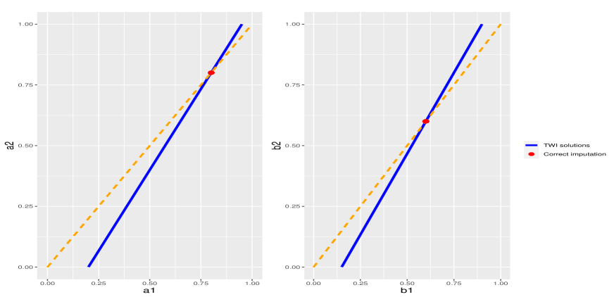
Nonetheless, (16) hints an additional requirement for the correct imputation, giving rise to the following condition.
- (C2)
-
Interpolator stability: , .
Intuitively, (C2) requires that, given the same neighboring observations, one should impute the missing entries in the same way (at least probabilistically) before and after . Together, (C1) and (C2) imply a unique solution to the system (17) and are sufficient for identification.
Proposition 7.
Under (C1) and (C2), the only solution to (17) is
That is, the only marginal distribution that achieves zero Wasserstein loss and satisfies (C2) is that of the underlying distribution.
As shown in Figure 1, the 45 degree line (dashed orange), which imposes (C2), intersects with the set of temporal Wasserstein imputations at the correct calibrations.
The above example illustrates when TWI can potentially identify the underlying marginal distribution. The crucial interpolator stability condition (C2) thus provides some guidance on the selection of TWI solutions. Indeed, Algorithm 1 may converge to varying solutions depending on the initialization. (C2) implies that we shall choose the solution so that the relationship between the imputed values and the neighboring observations stays stable before and after . In higher dimensions, summary statistics can be used. For example, fit a linear regression of imputed values on neighboring values using data before and after and compare the similarity of the coefficients. To promote interpolator stability, we suggest running TWI with different cut-off , using the previously obtained imputations as initializations. This leads to a simple procedure termed -TWI henceforth, which is summarized in Algorithm 2 below.
5 Simulation Studies
In this section, we apply the proposed temporal Wasserstein imputation to data generated from various time series models, including multivariate, nonlinear, and nonstationary ones, to examine its performance. For comparison, we employ alternative imputation methods such as Kalman smoothing, the scalar filtering algorithm of Peña and Tsay, (2021), and deterministic methods such as linear and spline interpolations. In addition, the following two missing patterns are considered.
-
Pattern I: 300 observations are omitted at random, which corresponds to sporadic missing data.
-
Pattern II: For every 20 observations, 6 consecutive observations are omitted, which mimics patches of missing data.
The total length of the time series is set to . Thus, for both missing patterns, 30% of the data are missing. For each model and missing pattern considered in this section, 1000 Monte Carlo simulations are carried out to compute the measure of performance.
We employ the proximal gradient descent (Parikh et al.,, 2014) to efficiently solve step (b) in Algorithm 1 when no side information is available since the projection step is straightforward. Conversely, when is defined by a system of linear equations, we solve step (b) using the closed form (7). In addition, we apply the -TWI (Algorithm 2) with three cut-off points (, , and ) to the simulated data. Both linear interpolation and Kalman smoothing are used as initialization of TWI in our experiments. Kalman smoothing and the deterministic smoothing techniques are implemented via the imputeTS package (Moritz and Bartz-Beielstein,, 2017) in R. The scalar filter algorithm (denoted as ScalarF henceforth) utilizes intervention analysis, and can be applied to multivariate and nonstationary series. The details are documented in Appendix B.
5.1 Linear and nonlinear univariate time series
In this subsection, we focus on univariate time series exhibiting linear or nonlinear dynamic patterns. Specifically, we consider the following time series models. In the sequel, and for denote i.i.d. sequences of standard Gaussian variables.
Model 1 (AR).
, where is set to 0.8.
Model 2 (ARMA).
, where is the backshift operator and .
Model 3 (TAR; Tong,, 1983).
where
Model 4 (I(1) process).
Data are generated according to
with .
Model 5 (Deterministic cyclic series with noise (CYC)).
Models 1 and 2 are linear time series models commonly seen in practice. Kalman smoothing is particularly adept at imputing such series. Note that Model 2 admits an AR() representation, so any finite-dimensional marginal distribution, the key objects TWI and -TWI work with, is inadequate to fully characterize the distribution of the underlying process. Model 3 is a celebrated threshold AR model which has found many applications in modeling nonlinear dynamics in the econometrics and statistics literature (Montgomery et al.,, 1998; Li and Ling,, 2012; Tsay and Chen,, 2018). Model 4 generates an I(1) series which typically produces a highly persistent stochastic trend. To remove the unit root, difference transform is usually applied to the data ; that is, one often deals with instead of the original series. However, this may result in excessive missing values in , which can cause difficulty in imputation. Finally, Model 5 features a deterministic cyclic trend with non-standard periods. Specifically, it includes two sinusoidal components with periods of 8.70 and 11.77, respectively.
Three measures of performance are considered. First, we report the Wasserstein distance (of order 2) between the empirical 3-dimensional marginal distributions of the imputed series and the full data. Specifically, let and be the imputed series and the original series in simulation , respectively, for . We report
| (18) |
as a measure of how well the imputed series approximates the original series. Second, we compare the root mean square estimation errors (RMSE) of the estimated autocovariance functions. Define , where and . Then the RMSE is defined as
| (19) |
where and with . Third, for Models 1–4, the model parameters are estimated using the imputed series, and their root mean square errors are reported.
The Wasserstein distance between the imputed and the original marginal distributions is reported in Table 1. Across all five models employed, the smallest loss is consistently achieved by TWI-type methods, indicating that TWI effectively approximates the distributional properties of the underlying series. While other methods may yield good imputations for some specific models, the result is not consistent across all models. For instance, linear and spline interpolations show low Wasserstein loss for Model 1, but their performance is less competitive when applied to other models. Similarly, the Kalman smoothing performs well under Model 1 with missing pattern I, but its advantage diminishes under missing pattern II. In contrast, TWI methods consistently deliver solid performance across models and missing patterns, provided they are carefully initialized.
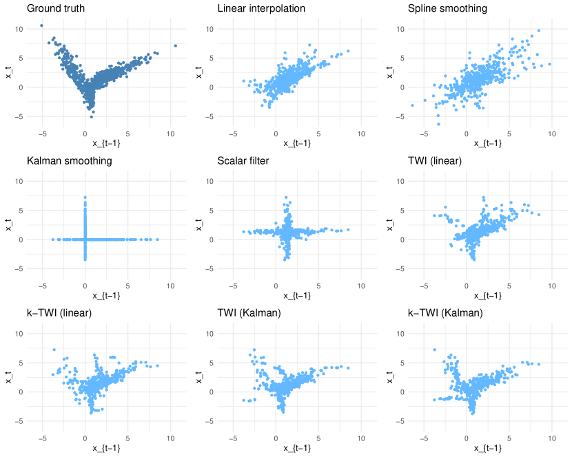
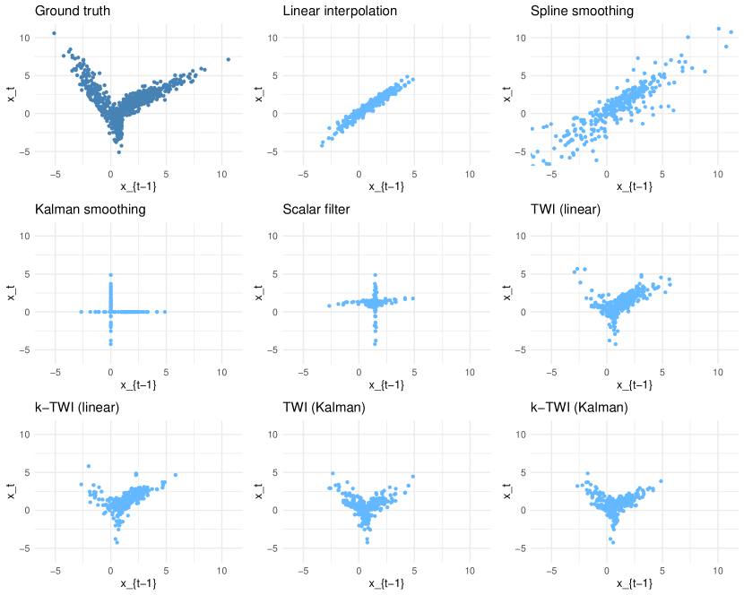
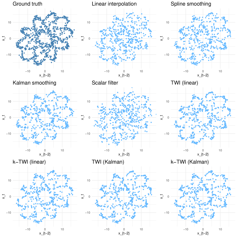
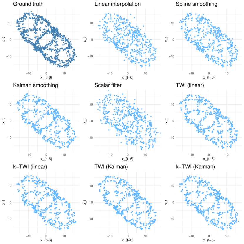
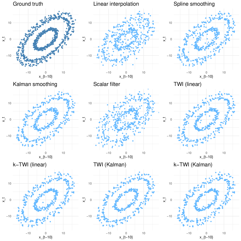
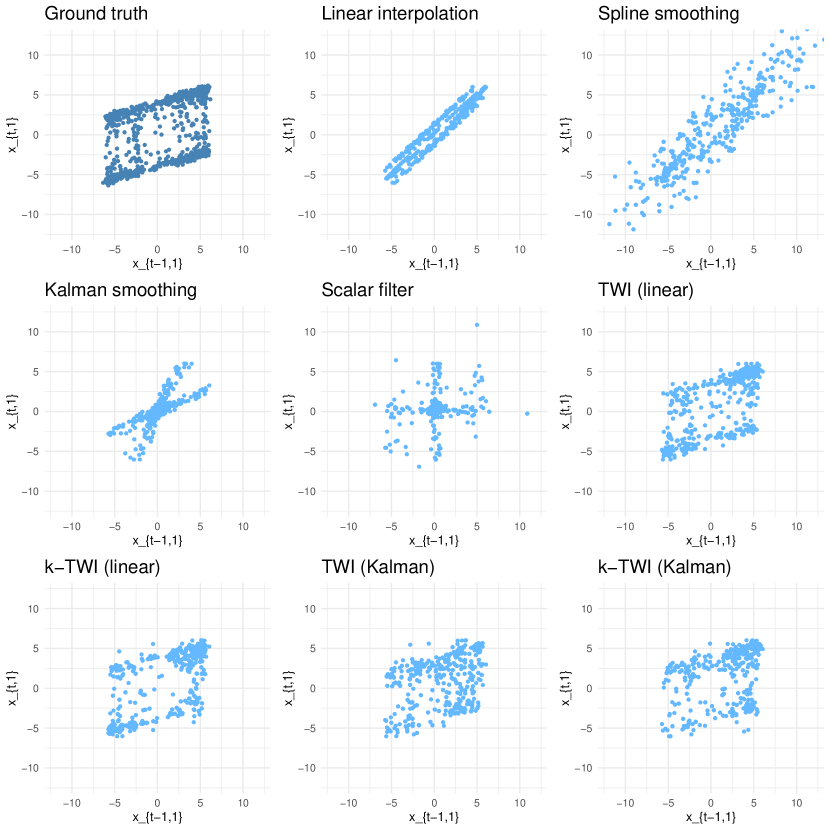
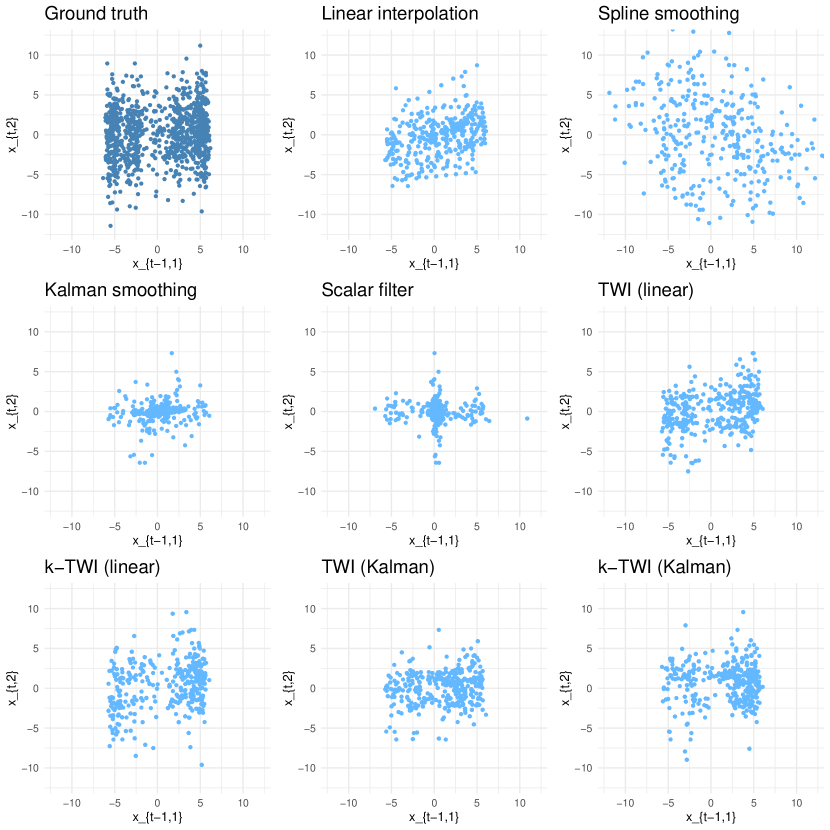
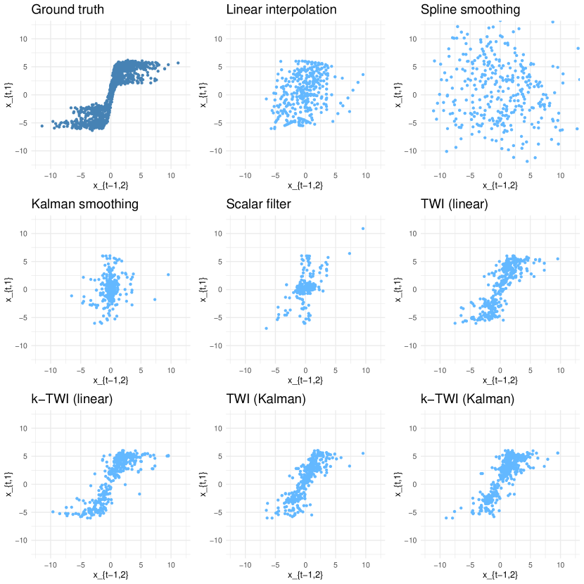
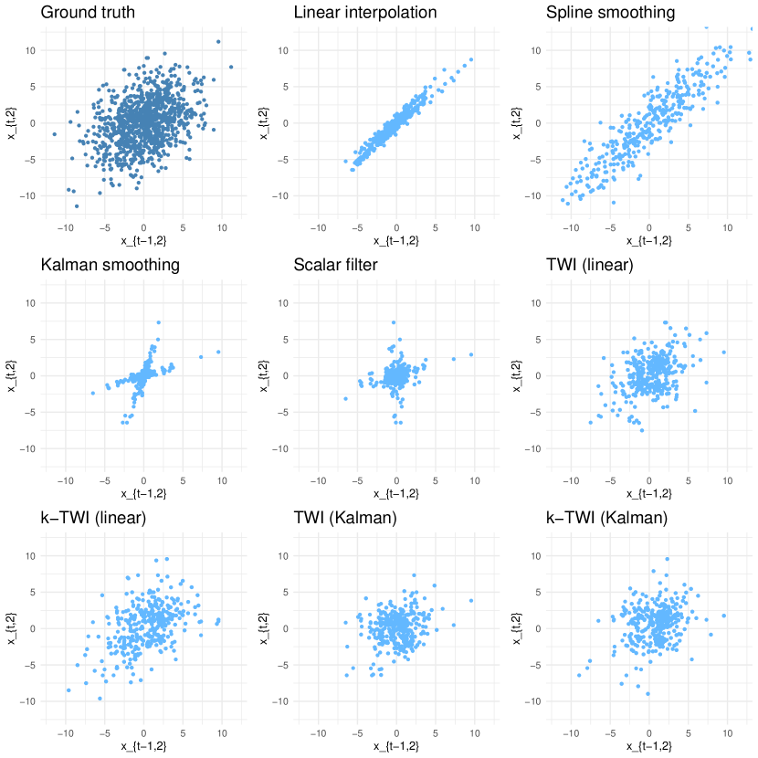
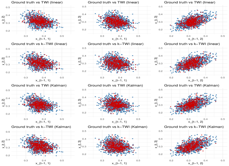
Additionally, Table 1 also shows TWI typically improves the Wasserstein loss from its initialization, often siginificantly. For example, for Model 3 (TAR), TWI reduces the Wasserstein loss from Kalman smoothing initialization by approximately 45% under missing pattern I (from 1.38 to 0.74). Similarly, for Model 5 (CYC), TWI reduces the Wasserstein loss by more than 50% from linear initialization (from 1.96 to 0.79). Figure 2 plots against when either or both are imputed ( or ) under Model 3, alongside of the original data. While Kalman smoothing introduces substantial distortion in the marginal distribution, TWI, initialized by Kalman smoothing, significantly corrects this bias, producing imputations that capture the nonlinearity in the ground truth. Figure 3 similarly plots against (and against ) for under Model 5. As shown in the figure, TWI markedly improves from its linear initialization by “denoising” the marginal distributions, leading to a distribution that closely match the ground truth.
For the nonstationary Model 4 (I(1)), we apply the methods to obtain an imputation and focus on the differenced series . Table 1 shows the Wasserstein distance between the marginal distributions implied by and . As noted before, there are many more missing values in than originally in . In this case, TWI still consistently yields the lowest Wasserstein loss and greatly improves from its initialization.
| Model | Linear | Spline | Kalman | ScalarF | TWIlin | -TWIlin | TWIKal | -TWIKal |
|---|---|---|---|---|---|---|---|---|
| Missing pattern I | ||||||||
| AR | 0.41 | 0.41 | 0.42 | 0.50 | 0.40 | 0.44 | 0.41 | 0.44 |
| ARMA | 0.48 | 0.58 | 0.47 | 0.48 | 0.40 | 0.38 | 0.40 | 0.38 |
| TAR | 1.12 | 1.51 | 1.38 | 1.13 | 0.96 | 0.81 | 0.74 | 0.63 |
| I(1) | 0.71 | 0.75 | 0.62 | 4.38 | 0.58 | 0.53 | 0.54 | 0.50 |
| CYC | 1.96 | 0.82 | 0.77 | 1.97 | 0.79 | 0.77 | 0.60 | 0.70 |
| NLVAR | 2.98 | 3.42 | 3.01 | 2.94 | 2.25 | 2.14 | 2.19 | 2.12 |
| ALR () | 0.70 | 1.00 | 4.17 | 0.55 | 0.43 | 0.37 | 0.38 | 0.35 |
| Missing pattern II | ||||||||
| AR | 0.44 | 0.59 | 0.50 | 0.76 | 0.39 | 0.44 | 0.43 | 0.45 |
| ARMA | 0.47 | 1.29 | 0.51 | 0.53 | 0.36 | 0.34 | 0.40 | 0.35 |
| TAR | 1.04 | 3.11 | 1.25 | 0.99 | 0.84 | 0.73 | 0.76 | 0.61 |
| I(1) | 0.67 | 0.65 | 0.60 | 8.35 | 0.51 | 0.45 | 0.49 | 0.44 |
| CYC | 2.58 | 1.81 | 0.77 | 3.79 | 2.62 | 1.60 | 0.62 | 0.72 |
| NLVAR | 3.00 | 6.07 | 3.33 | 3.67 | 2.13 | 2.02 | 2.31 | 2.04 |
| ALR () | 0.56 | 1.83 | 3.81 | 0.46 | 0.36 | 0.33 | 0.40 | 0.34 |
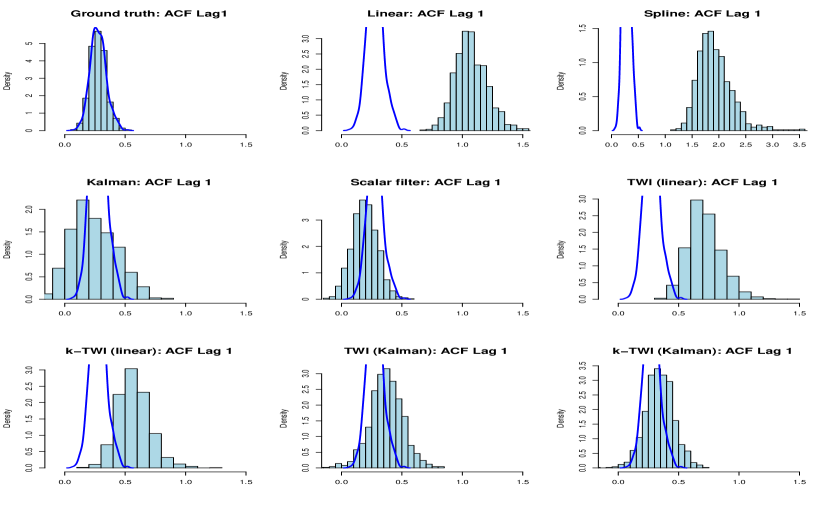
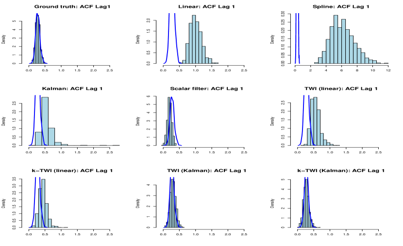
Next, we examine the sample autocovariance functions (ACFs) estimated from the imputed data. Table 2 reports for . For Model 1 (AR), most methods perform reasonably well. Linear interpolation produces accurate ACF estimates since the positive AR coefficient intrinsically favors linearity, while the scalar filter exhibits largest estimation errors. For Model 2 (ARMA), TWI improves from linear and Kalman initializations and yields more accurate ACF estimates: TWI reduces the biases in Kalman smoothing when and in linear interpolation when , and . For the nonlinear Model 3 (TAR), the ACFs estimated from the TWI-imputed series exhibit the lowest RMSEs, with substantial improvements over the initializations. Notably, the scalar filter also yields accurate ACFs for . Figure 4 plots the histogram of the estimated ACFs at lag 1 (that is, ), which shows how TWI effectively nullifies the biases caused by the initializations.
The advantage of TWI becomes even more pronounced in nonstationary models 4 (I(1)) and 5 (CYC), for which it achieves low ACF estimation errors. The scalar filter performs poorly for these models, which is likely the consequence of using many indicators in the intervention analysis. Among the benchmarks, Kalman filter produces the best result for these two models, but it can be further improved by the proposed TWI procedure.
| Model | Linear | Spline | Kalman | ScalarF | TWIlin | -TWIlin | TWIKal | -TWIKal | |
|---|---|---|---|---|---|---|---|---|---|
| Missing pattern I | |||||||||
| AR | 0 | 0.32 | 0.29 | 0.37 | 0.50 | 0.30 | 0.31 | 0.32 | 0.32 |
| 1 | 0.26 | 0.34 | 0.29 | 0.47 | 0.27 | 0.30 | 0.28 | 0.31 | |
| 2 | 0.26 | 0.27 | 0.29 | 0.38 | 0.25 | 0.28 | 0.27 | 0.29 | |
| ARMA | 0 | 0.14 | 0.19 | 0.29 | 0.31 | 0.13 | 0.13 | 0.22 | 0.18 |
| 1 | 0.22 | 0.44 | 0.07 | 0.08 | 0.14 | 0.10 | 0.07 | 0.07 | |
| 2 | 0.08 | 0.08 | 0.07 | 0.07 | 0.06 | 0.06 | 0.07 | 0.07 | |
| TAR | 0 | 0.59 | 0.77 | 0.73 | 1.07 | 0.65 | 0.56 | 0.56 | 0.45 |
| 1 | 0.81 | 1.68 | 0.19 | 0.14 | 0.46 | 0.32 | 0.17 | 0.13 | |
| 2 | 0.40 | 0.31 | 0.16 | 0.11 | 0.24 | 0.16 | 0.10 | 0.09 | |
| I(1) | 0 | 0.52 | 0.40 | 0.48 | 19.41 | 0.42 | 0.35 | 0.40 | 0.34 |
| 1 | 0.35 | 0.51 | 0.25 | 9.32 | 0.28 | 0.25 | 0.22 | 0.21 | |
| 2 | 0.17 | 0.35 | 0.11 | 1.28 | 0.15 | 0.14 | 0.11 | 0.11 | |
| CYC | 0 | 10.94 | 2.40 | 3.90 | 4.67 | 1.81 | 1.25 | 0.68 | 0.62 |
| 1 | 9.05 | 1.72 | 3.33 | 5.88 | 1.47 | 1.04 | 0.54 | 0.51 | |
| 2 | 1.90 | 0.46 | 0.81 | 2.13 | 0.41 | 0.33 | 0.17 | 0.18 | |
| Missing pattern II | |||||||||
| AR | 0 | 0.38 | 0.70 | 0.55 | 0.78 | 0.33 | 0.36 | 0.43 | 0.39 |
| 1 | 0.28 | 0.79 | 0.42 | 0.70 | 0.29 | 0.34 | 0.37 | 0.36 | |
| 2 | 0.26 | 0.66 | 0.36 | 0.65 | 0.27 | 0.31 | 0.34 | 0.34 | |
| ARMA | 0 | 0.14 | 1.35 | 0.31 | 0.32 | 0.13 | 0.11 | 0.24 | 0.17 |
| 1 | 0.17 | 1.49 | 0.08 | 0.09 | 0.10 | 0.08 | 0.07 | 0.07 | |
| 2 | 0.15 | 1.05 | 0.07 | 0.08 | 0.09 | 0.07 | 0.07 | 0.07 | |
| TAR | 0 | 0.49 | 5.39 | 0.71 | 1.08 | 0.72 | 0.68 | 0.73 | 0.65 |
| 1 | 0.75 | 6.04 | 0.34 | 0.11 | 0.31 | 0.20 | 0.09 | 0.09 | |
| 2 | 0.77 | 4.36 | 0.34 | 0.10 | 0.42 | 0.28 | 0.19 | 0.14 | |
| I(1) | 0 | 0.47 | 0.27 | 0.47 | 51.84 | 0.38 | 0.30 | 0.36 | 0.29 |
| 1 | 0.19 | 0.43 | 0.18 | 0.56 | 0.17 | 0.14 | 0.14 | 0.13 | |
| 2 | 0.08 | 0.08 | 0.07 | 0.52 | 0.08 | 0.08 | 0.07 | 0.07 | |
| CYC | 0 | 7.46 | 7.56 | 1.96 | 15.21 | 12.27 | 6.49 | 1.26 | 1.03 |
| 1 | 2.63 | 3.99 | 1.45 | 16.23 | 9.57 | 5.07 | 0.98 | 0.83 | |
| 2 | 11.18 | 5.09 | 0.79 | 7.90 | 1.28 | 1.04 | 0.28 | 0.31 | |
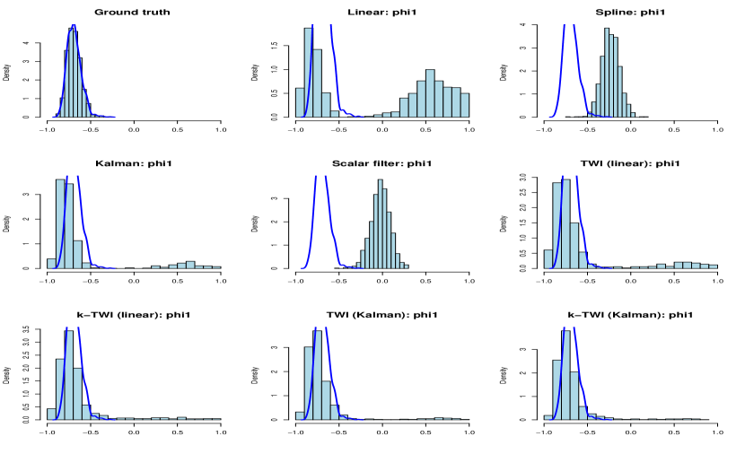
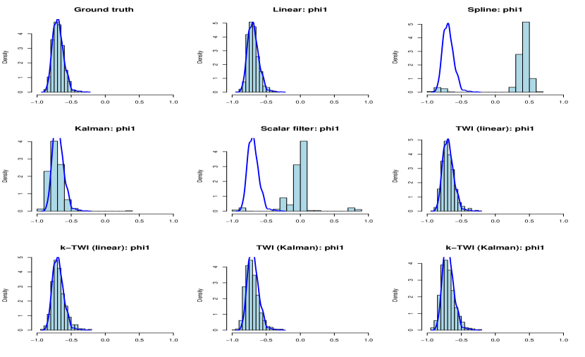
Finally, we turn to the model parameters estimated from the imputed series. Table 3 presents the RMSEs for each model parameter. For Model 1 (AR) and Model 2 (ARMA), Kalman smoothing and the scalar filter yield satisfactory estimates among the benchmarks, with TWI offering only limited improvements. For the nonlinear Model 3 (TAR), the results are drastically different. TWI produces the most accurate parameter estimates and can achieve approximately 50% reduction in estimation errors compared to linear interpolation and Kalman smoothing. In some cases, such as with linear initialization under missing pattern II, the improvement far exceeds 50%. These estimation results demonstrate TWI’s strength in learning the underlying nonlinear dynamics. For Model 4 (I(1)), TWI either outperforms or stays on par with the best benchmark, with Kalman filter being a strong initialization. Figure 5 shows the histogram of the estimated parameter in Model 4. It is visible from the figure that TWI helps neutralize the biases from the initialization and produces reliable estimates.
| Model | Linear | Spline | Kalman | ScalarF | TWIlin | -TWIlin | TWIKal | -TWIKal | |
|---|---|---|---|---|---|---|---|---|---|
| Missing pattern I | |||||||||
| AR | 0.06 | 0.06 | 0.05 | 0.03 | 0.03 | 0.04 | 0.03 | 0.04 | |
| ARMA | 0.19 | 0.47 | 0.12 | 0.08 | 0.17 | 0.16 | 0.11 | 0.11 | |
| 0.46 | 0.95 | 0.18 | 0.10 | 0.33 | 0.26 | 0.16 | 0.15 | ||
| TAR | 1.02 | 1.67 | 0.82 | 0.63 | 0.71 | 0.58 | 0.53 | 0.44 | |
| 0.08 | 0.07 | 0.20 | 0.04 | 0.05 | 0.03 | 0.03 | 0.02 | ||
| 0.01 | 0.75 | 0.35 | 0.20 | 0.05 | 0.05 | 0.03 | 0.03 | ||
| I(1) | 0.96 | 0.47 | 0.45 | 0.68 | 0.48 | 0.32 | 0.30 | 0.24 | |
| NLVAR | 0.19 | 0.27 | 0.15 | 0.03 | 0.06 | 0.03 | 0.05 | 0.03 | |
| 3.10 | 3.16 | 2.87 | 1.67 | 1.34 | 1.02 | 1.22 | 0.97 | ||
| 0.03 | 0.07 | 0.03 | 0.03 | 0.03 | 0.03 | 0.03 | 0.03 | ||
| 0.18 | 0.23 | 0.10 | 0.04 | 0.05 | 0.04 | 0.04 | 0.04 | ||
| Missing pattern II | |||||||||
| AR | 0.05 | 0.07 | 0.04 | 0.04 | 0.03 | 0.02 | 0.03 | 0.02 | |
| ARMA | 0.04 | 0.08 | 0.09 | 0.08 | 0.05 | 0.06 | 0.09 | 0.09 | |
| 0.16 | 0.61 | 0.11 | 0.10 | 0.12 | 0.11 | 0.11 | 0.12 | ||
| TAR | 0.72 | 2.44 | 0.38 | 0.25 | 0.25 | 0.20 | 0.29 | 0.21 | |
| 0.09 | 0.12 | 0.05 | 0.03 | 0.06 | 0.05 | 0.02 | 0.01 | ||
| 0.01 | 1.72 | 0.01 | 0.01 | 0.01 | 0.01 | 0.01 | 0.01 | ||
| I(1) | 0.08 | 1.08 | 0.11 | 0.70 | 0.09 | 0.10 | 0.10 | 0.10 | |
| NLVAR | 0.19 | 0.44 | 0.08 | 0.02 | 0.02 | 0.01 | 0.02 | 0.01 | |
| 2.67 | 3.51 | 1.68 | 1.26 | 0.61 | 0.46 | 0.61 | 0.43 | ||
| 0.02 | 0.09 | 0.03 | 0.03 | 0.06 | 0.05 | 0.04 | 0.03 | ||
| 0.15 | 0.34 | 0.05 | 0.04 | 0.04 | 0.04 | 0.04 | 0.04 | ||
In conclusion, under the univariate time series models considered in this subsection, which include linear, nonlinear, and nonstationary time series, TWI consistently fares well in all three comparing metrics. It can capture nonlinear dynamics as illustrated by the low Wasserstein error in the imputed marginal distributions, which provides substantial improvements in downstream ACF and model estimates.
5.2 Multivariate time series
In this subsection, we consider the following two multivariate nonlinear time series models.
Model 6 (Nonlinear VAR; NLVAR).
where is the centered sigmoid function, and .
Model 7 (Additive logistic model; AL, Brunsdon and Smith,, 1998).
and the observed data are
Model 6 is a VAR model with a nonlinear term. In particular, the impact of on is nonlinear and is modeled by a sigmoid function. Model 7 generates the so-called compositional time series, which refers to a multivariate time series , where , , such that for each , , and for all . Such data are encountered in a wide array of fields such as the environmental sciences, economics, geology and political science. Here, we adopt the additive logistic (AL) model of Brunsdon and Smith, (1998) in Model 7. The AL model postulates that after some nonlinear transformation, the data follow a standard VARMA model. In fact, one can view compositional data as a time series on some low-dimensional manifold. Alternative models for composition time series include the recent works of Zheng and Chen, (2017), Harvey et al., (2024), and Zhu and Müller, (2024).
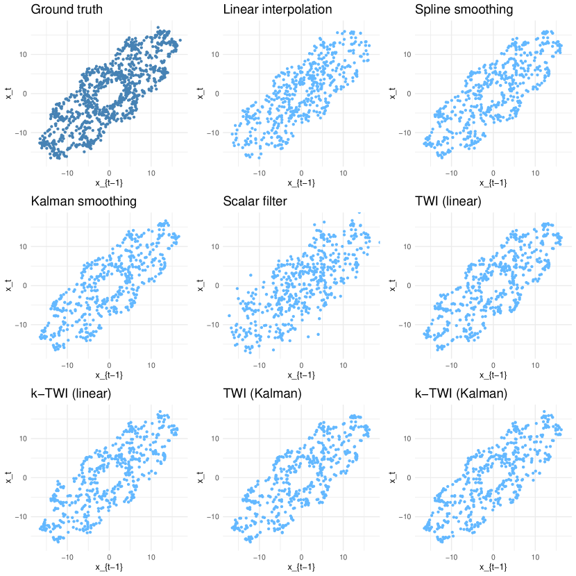
Focus on Model 6 (NLVAR) first. The Wasserstein distances between the 3-dimensional marginal distributions of the imputed and the original series, defined in (18), are again reported Table 1. TWI methods clearly produce the lowest Wasserstein distances. As depicted in Figure 6, TWI successfully captures the underlying nonlinear dynamics, whereas other imputation methods fail to preserve meaningful relationships. Next, we assess the effectiveness of the imputed series in estimating the model parameters, assuming the nonlinearity is known. That is, we estimate by plugging in the imputed series. The root mean square estimation errors are documented in Table 3. Compared to the benchmarks, TWI provides considerable error reduction in the parameter associated with the nonlinear effect, . It attains more than 50% reduction in RMSE from initialization under both missing patterns I and II, and can achieve 50% lower RMSE than the scalar filter, the best-performing benchmark.
Next, we turn to Model 7 (AL). Since the components must sum to unity, they exhibit negative correlation when one component approaches the endpoints 0 and 1. However, such correlation tends to weaken when the series are near the midpoint. Table 1 records the Wasserstein distance between the 3-dimensional marginal distribution of the imputed and original series. With the smallest Wasserstein loss, TWI methods again demonstrate their ability to adapt to nonlinear dependence structures.
It is worth noting that while the linear interpolation results in a compositional series, other methods, such as the Kalman smoothing, do not generally maintain this compositional property. By restricting the admissible set, TWI ensures that the imputed series remain compositional. As shown in Figure 7, linear interpolation falsely promotes negative correlation between and and Kalman smoothing often deviates from the plausible range of a compositional series. TWI amends these peculiarities, leading to imputations that align more closely with the underlying data.
6 Groundwater data application
In this section, we apply the proposed temporal Wasserstein imputation to a groundwater dataset from Taiwan. Groundwater serves as a critical water source for Taiwan, and its management is of considerable importance to the policymakers as well as the industrial sector, particularly due to the island’s steep topography and varying rainfall distribution (Hsu et al.,, 2020). However, the statistical analysis of groundwater levels is challenged by frequent missing data, especially from deeper wells. To address this, imputation of missing values is essential to facilitate reliable downstream analyses.
6.1 Preprocessing and exploratory analysis
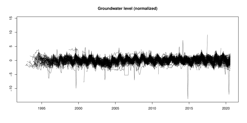
Our goal is to study the seasonal groundwater variations, for which we first transform the data into monthly records. The data contain hourly observations from 352 monitoring sites between October, 1992 and August, 2020. For each site, we define monthly groundwater level by the average of the observations in a given month. If more than one-third of the observations for a month are missing, we classify that month as missing. For our analysis, we focus on sites with a less-than-median amount of missing data, reducing the sample to 176 sites. Figure 8 shows the monthly groundwater levels for these sites, after subtracting the mean and normalized by the standard deviation. We make two observations. First, many series exhibit strong seasonality, which is due to the rainfall pattern in Taiwan. There is more rain in the summer due to monsoon and typhoons, while winters are generally drier. Second, there are many outlying values and anomalies in the observed series. For instance, there are abrupt changes in groundwater levels that are more than 5 standard deviations from the sample mean. For the purpose of our analysis, we treat such extreme values as missing data.
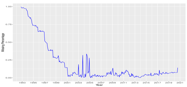
During the period from October, 1992 to August, 2020, few months recorded valid observations at all sites. Figure 9 shows the fluctuations in the percentage of sites with missing data over time. Although missing data are mostly prevalent in the early years with more than 50% of the sites generating missing data, there are some time during which the percentage surges, such as between 2003 and 2005. In addition, the percentage of missing data is gradually increasing in more recent years. Thus, one may lose much information if the analysis is restricted to sites with relatively complete records.
6.2 Results
Similar to Section 5, we employ linear interpolation, spline interpolation, Kalman smoothing, and the scalar filter as benchmark imputation methods. For TWI and -TWI, linear interpolation and Kalman smoothing are again used as initializations.
We consider two downstream tasks using the imputed series. First, we perform dimension reduction via the time series factor model of Lam et al., (2011). The factor model postulates that the observations are driven by a small number of latent factor processes. Specifically,
where , , is the factor process and is white noise. Factor modeling is helpful for understanding the high-dimensional time series and its complex temporal patterns. However, estimating the factor model requires eigenanalysis of the autocovariance matrices , which becomes infeasible when the series are severely corrupted by missing data.
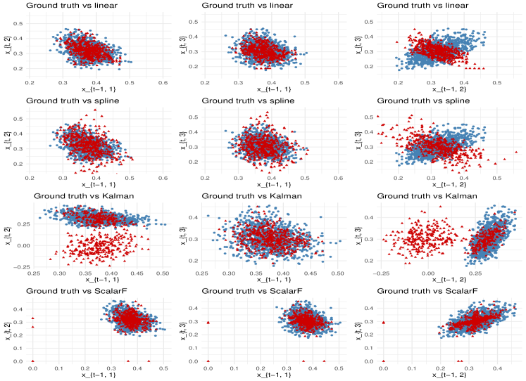
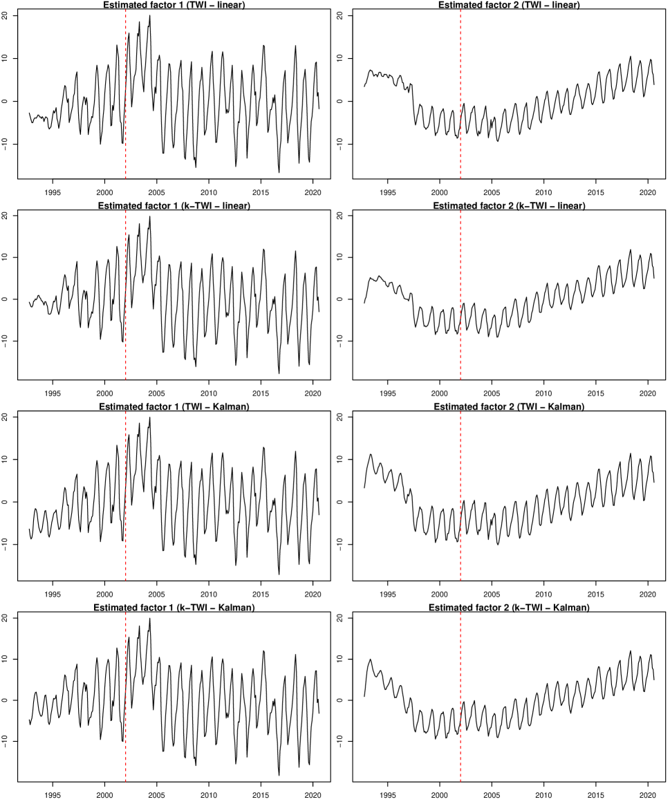
Figure 10 shows the leading two factors estimated using series imputed by the benchmark methods. The linear and spline interpolation methods, both favoring trend preservation, result in the first estimated factor displaying strong trends, while the second factor reflects more the seasonal patterns. Notably, this is reversed when factors are estimated based on series imputed by Kalman smoothing and scalar filter. In these cases, the leading factor process exhibits strong seasonality, and the second factor displays trend patterns with a slight U-shape, which is quite different from those estimated with linear and spline methods.
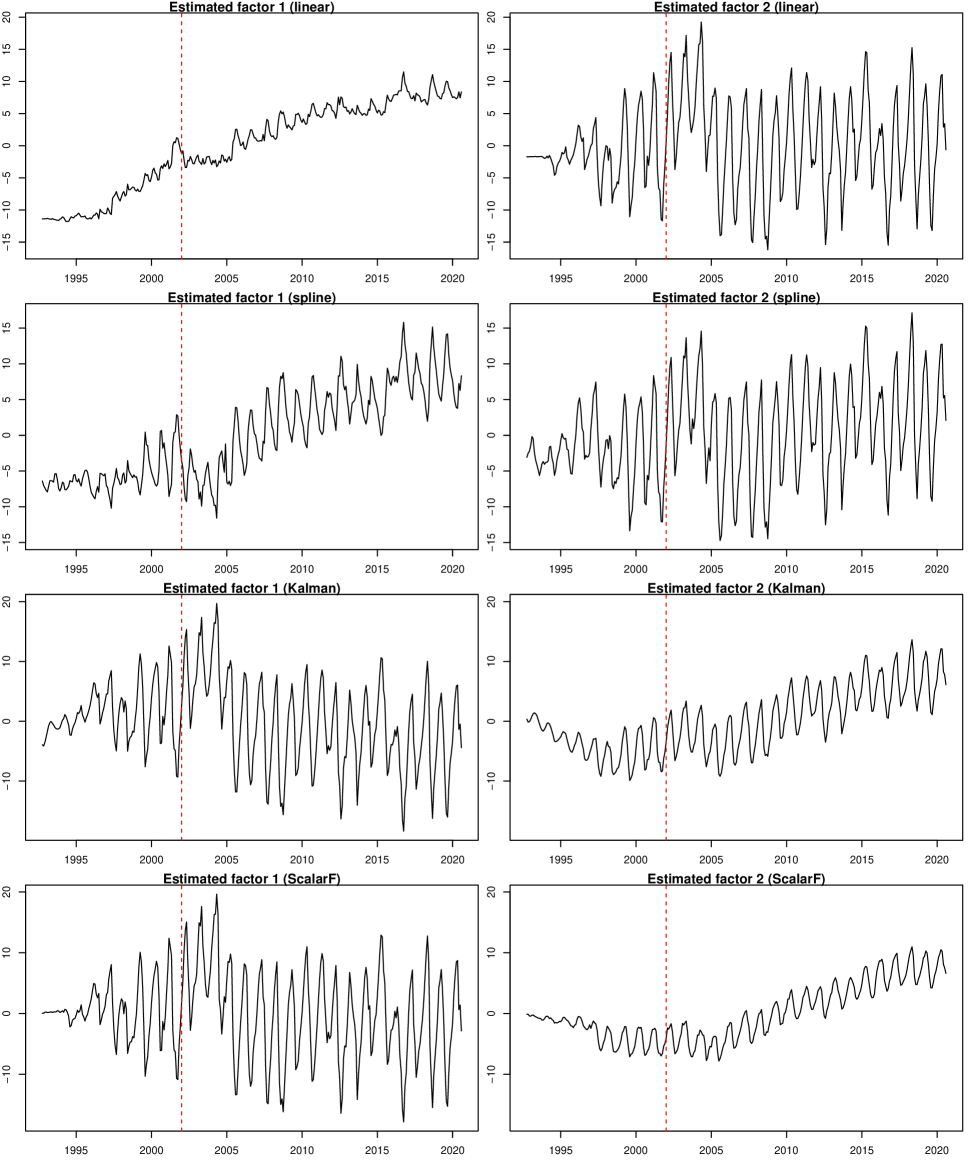
Figure 11 displays the leading two factors estimated using series imputed by TWI and -TWI. Note that while linear interpolation has led to a strong trend factor, as shown in Figure 10, the leading estimated factor of TWI initialized by linear interpolations exhibits significant seasonal pattern, which aligns more closely with those estimated by Kalman smoothing and scalar filter. Moreover, the second estimated factor also shows trends resembling those of the Kalman smoothing and scalar filter, but with a more apparent U-shape. To compare TWI with Kalman smoothing, we focus on the data before January 2002 (marked by the red dashed lines in Figure 10 and 11). Recall that missing data are prevalent during this period (Figure 9). Factors estimated by Kalman smoothing are affected by the abundance of missing data and tend to show smaller variations in the early periods, which may be the result of small variances in the optimal interpolator. In contrast, factors estimated using data imputed by TWI (initialized by Kalman smoothing) show consistent variational patterns across time and appear more trustworthy in understanding the dynamics. Overall, TWI took a more holistic view of the series which accounts for the prominent seasonality and trend in the data.
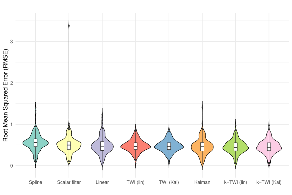
Our second downstream task concerns autoregreesive modeling. Specifically, we fit an AR(6) model using data imputed by the methods considered. The training data consists of the early period between October, 1992 and September, 2002, amounting to 120 data points per series, including missing values. Then, we assess the impact of imputation quality by the out-of-sample prediction performance in predicting the remaining data. Note that the missing data in the test data are removed for fair comparison. Figure 12 presents, in violin plots, the distribution of the root mean squared prediction errors (RMSE) for each method across the 176 series under study. The TWI-type methods effectively alleviate the large RMSEs caused by the benchmark imputation methods and produce lower RMSEs in general.
In conclusion, the temporal Wasserstein imputation preserves important temporal features such as the seasonal patterns and enables complex downstream statistical analyses such as factor modeling. Our analysis show that the results obtained from TWI appear reliable. Thus, we expect the series imputed by TWI are also suitable for further analyses, especially when nonlinear models are employed.
7 Conclusion
In this work, we proposed an imputation method, the temporal Wasserstein imputation, for imputing missing entries in time series data. The proposed method complements the existing approaches by effectively capturing nonlinear dynamics and reducing the distributional bias typically observed for the conventional methods in handling missing time series data. Hence, the imputation of the proposed method is more reliable in downstream analysis. Our simulation studies and the analysis of groundwater data support the practical utility of the proposed method.
Appendix A Proof of Proposition 6
Lemma 8.
Suppose satisfies (A1) and (A2). Then
where .
Proof.
By Theorem 7.12 of Villani, (2021), it suffices to show that with probability one,
| (20) |
and
| (21) |
By Theorem 36.4 of Billingsley, (1995), the processes and are stationary and ergodic for any , where . Thus (21) follows immediately from the Ergodic theorem. To show (20), it suffices to show, with probability one,
By the Ergodic theorem, we have
| (22) |
with probability one. Let
noting that by (A2). By the Ergodic theorem and (22), . Fix and let and be arbitrary. Since is uniformly continuous, there exists such that
| (23) |
for all with . In addition, using , we have
| (24) |
for all , such that . Combining (23)–(24), we have
on . Note, in particular, that and do not depend on . Letting and proves (20) holds on , and hence with probability one. ∎
Appendix B Scalar filter algorithm
The following summarizes the scalar filter algorithm of Peña and Tsay, (2021).
-
•
Initialize the imputation with if .
-
•
For each , let be the indicator function. That is,
and estimate the intervention model using . For example, one can fit an ARX model with as exogenous predictors.
-
•
Let be the intervention effect associated with . Estimate the missing data by
As one can see from the algorithm above, the scalar filter algorithm proposed by Peña and Tsay, (2021) is based on intervention analysis. It can be iterated in order to improve the estimates. However, no convergence guarantee is provided by the authors.
When fitting an ARX model with the indicators as exogenous predictors, if there are many missing values, standard approaches may be infeasible or unreliable due to near collinearity. In this case, we employ a small penalty to avoid numerical instability.
References
- Alonso and Sipols, (2008) Alonso, A. M. and Sipols, A. E. (2008). A time series bootstrap procedure for interpolation intervals. Computational Statistics & Data Analysis, 52(4):1792–1805.
- Ambrosio et al., (2006) Ambrosio, L., Gigli, N., and Savare, G. (2006). Gradient Flows: In Metric Spaces and in the Space of Probability Measures. Lectures in Mathematics. ETH Zürich. Birkhäuser Basel.
- Bertsekas, (1992) Bertsekas, D. (1992). Auction algorithms for network flow problems: A tutorial introduction. Computational Optimization and Applications, 1:7–66.
- Billingsley, (1995) Billingsley, P. (1995). Probability and Measure. Wiley Series in Probability and Statistics. Wiley.
- Boyd and Vandenberghe, (2004) Boyd, S. and Vandenberghe, L. (2004). Convex Optimization. Cambridge University Press.
- Brenier, (1987) Brenier, Y. (1987). Décomposition polaire et réarrangement monotone des champs de vecteurs. CR Acad. Sci. Paris Sér. I Math., 305:805–808.
- Brunsdon and Smith, (1998) Brunsdon, T. M. and Smith, T. (1998). The time series analysis of compositional data. Journal of Official Statistics, 14(3):237–253.
- Carrizosa et al., (2013) Carrizosa, E., Olivares-Nadal, A. V., and Ramírez-Cobo, P. (2013). Time series interpolation via global optimization of moments fitting. European Journal of Operational Research, 230(1):97–112.
- Cuturi, (2013) Cuturi, M. (2013). Sinkhorn distances: Lightspeed computation of optimal transport. In Advances in Neural Information Processing Systems, volume 26.
- Deb et al., (2021) Deb, N., Ghosal, P., and Sen, B. (2021). Rates of estimation of optimal transport maps using plug-in estimators via barycentric projections. In Advances in Neural Information Processing Systems, volume 34, pages 29736–29753.
- Galichon, (2016) Galichon, A. (2016). Optimal Transport Methods in Economics. Princeton University Press.
- Galichon, (2021) Galichon, A. (2021). The unreasonable effectiveness of optimal transport in economics. preprint. hal-03936221.
- Gómez et al., (1999) Gómez, V., Maravall, A., and Peña, D. (1999). Missing observations in arima models: Skipping approach versus additive outlier approach. Journal of Econometrics, 88(2):341–363.
- Grippo and Sciandrone, (2000) Grippo, L. and Sciandrone, M. (2000). On the convergence of the block nonlinear gauss–seidel method under convex constraints. Operations Research Letters, 26(3):127–136.
- Harvey et al., (2024) Harvey, A., Hurn, S., Palumbo, D., and Thiele, S. (2024). Modelling circular time series. Journal of Econometrics, 239(1):105450.
- Harvey and Pierse, (1984) Harvey, A. C. and Pierse, R. G. (1984). Estimating missing observations in economic time series. Journal of the American Statistical Association, 79(385):125–131.
- Hastie et al., (2009) Hastie, T., Tibshirani, R., and Friedman, J. (2009). The Elements of Statistical Learning: Data Mining, Inference, and Prediction. Springer series in statistics. Springer New York, NY.
- Hsu et al., (2020) Hsu, Y.-J., Fu, Y., Bürgmann, R., Hsu, S.-Y., Lin, C.-C., Tang, C.-H., and Wu, Y.-M. (2020). Assessing seasonal and interannual water storage variations in taiwan using geodetic and hydrological data. Earth and Planetary Science Letters, 550:116532.
- Lam et al., (2011) Lam, C., Yao, Q., and Bathia, N. (2011). Estimation of latent factors for high-dimensional time series. Biometrika, 98(4):901–918.
- Li and Ling, (2012) Li, D. and Ling, S. (2012). On the least squares estimation of multiple-regime threshold autoregressive models. Journal of Econometrics, 167(1):240–253.
- Little and Rubin, (2019) Little, R. and Rubin, D. (2019). Statistical Analysis with Missing Data. Wiley Series in Probability and Statistics. Wiley.
- McCann, (1995) McCann, R. J. (1995). Existence and uniqueness of monotone measure-preserving maps. Duke Mathematical Journal, 80(2):309–323.
- Montgomery et al., (1998) Montgomery, A. L., Zarnowitz, V., Tsay, R. S., and Tiao, G. C. (1998). Forecasting the u.s. unemployment rate. Journal of the American Statistical Association, 93(442):478–493.
- Moritz and Bartz-Beielstein, (2017) Moritz, S. and Bartz-Beielstein, T. (2017). imputeTS: Time series missing value imputation in r. The R Journal, 9(1):207–218.
- Orlin, (1997) Orlin, J. B. (1997). A polynomial time primal network simplex algorithm for minimum cost flows. Mathematical Programming, 78:109–129.
- Parikh et al., (2014) Parikh, N., Boyd, S., et al. (2014). Proximal algorithms. Foundations and trends® in Optimization, 1(3):127–239.
- Peña and Maravall, (1991) Peña, D. and Maravall, A. (1991). Interpolation, outliers and inverse autocorrelations. Communications in Statistics - Theory and Methods, 20(10):3175–3186.
- Peña et al., (2011) Peña, D., Tiao, G., and Tsay, R. (2011). A Course in Time Series Analysis. Wiley Series in Probability and Statistics. Wiley.
- Peña and Tsay, (2021) Peña, D. and Tsay, R. (2021). Statistical Learning for Big Dependent Data. Wiley Series in Probability and Statistics. Wiley.
- Peyré and Cuturi, (2019) Peyré, G. and Cuturi, M. (2019). Computational Optimal Transport: With Applications to Data Science. Foundations and trends in machine learning. Now Publishers.
- Pourahmadi, (1989) Pourahmadi, M. (1989). Estimation and interpolation of missing values of a stationary time series. Journal of Time Series Analysis, 10(2):149–169.
- Tong, (1983) Tong, H. (1983). Threshold Models in Nonlinear Time Series Analysis. Lecture Notes in Statistics. Springer New York, NY.
- Tsay and Chen, (2018) Tsay, R. and Chen, R. (2018). Nonlinear Time Series Analysis. Wiley Series in Probability and Statistics. Wiley.
- Villani, (2008) Villani, C. (2008). Optimal Transport: Old and New. Grundlehren der mathematischen Wissenschaften. Springer Berlin, Heidelberg.
- Villani, (2021) Villani, C. (2021). Topics in Optimal Transportation. Graduate Studies in Mathematics. American Mathematical Society.
- Zheng and Chen, (2017) Zheng, T. and Chen, R. (2017). Dirichlet arma models for compositional time series. Journal of Multivariate Analysis, 158:31–46.
- Zhu and Müller, (2024) Zhu, C. and Müller, H.-G. (2024). Spherical autoregressive models, with application to distributional and compositional time series. Journal of Econometrics, 239(2):105389.