Automorphism-Assisted Quantum Approximate Optimization Algorithm for efficient graph optimization

Abstract

In this article we report on the application of the Quantum Approximate Optimization Algorithm (QAOA) to solve the unweighted MaxCut problem on tree-structured graphs. Specifically, we utilize the Nauty (No Automorphisms, Yes?) package to identify graph automorphisms, focusing on determining edge equivalence classes. These equivalence classes also correspond to symmetries in the terms of the associated Ising Hamiltonian. By exploiting these symmetries, we achieve a significant reduction in the complexity of the Hamiltonian, thereby facilitating more efficient quantum simulations. We conduct benchmark experiments on graphs with up to 34 nodes on memory and CPU intensive TPU provided by google Colab, applying QAOA with a single layer (p=1). The approximation ratios obtained from both the full and symmetry-reduced Hamiltonians are systematically compared. Our results show that using automorphism-based symmetries to reduce the Pauli terms in the Hamiltonian can significantly decrease computational overhead without compromising the quality of the solutions obtained.

1 Introduction

The Quantum Approximate Optimization Algorithm (QAOA), introduced by Farhi et al.[1], has become a leading method for addressing NP-hard combinatorial optimization challenges on near-term quantum devices. As a hybrid quantum-classical algorithm, QAOA optimizes a parameterized quantum circuit through variational techniques, exploring solution spaces by alternating unitaries informed by problem-specific Hamiltonians. This approach presents a robust framework for efficiently solving complex optimization problems like MaxCut, where classical solutions are often computationally prohibitive due to the exponential search space associated with all potential graph cuts.

In the context of the unweighted MaxCut problem, QAOA constructs a Hamiltonian that encodes graph connectivity, with each term corresponding to an edge that signifies whether adjacent vertices belong to the same partition. Recent research has focused on enhancing the efficiency of QAOA, addressing the algorithm’s computational demands and improving performance on large-scale instances[2, 3, 4, 5, 6, 7, 8, 9]. A primary bottleneck in QAOA lies in optimizing gate parameters, which scales significantly with the number of qubits even at minimal circuit depths (e.g., single Trotterized layer). Consequently, leveraging graph symmetries, especially automorphisms[10, 11, 12, 13, 14], has emerged as a promising strategy. Automorphisms are bijective mappings that preserve graph structure, enable the identification of equivalence classes among graph edges, thus reducing redundancy within the solution space. For instance, [15] explores an automorphism-based simplification that calculates optimal gate parameters via the Reverse Causal Cone (RCC). This method identifies edge equivalence classes based on automorphism group generators $Aut(G)$, and computes the ground-state energy classically using tensor-netwroks for each of the RCC subgraph associated with a representative edge from each equivalence class. Automorphisms are computed using the highly efficient Nauty (No Automorphisms, Yes?) package, developed by McKay and Piperno[16], which is widely used for automorphism computations in complex graph structures. Building on these principles, we propose an Automorphism-Assisted QAOA (AA-QAOA) that integrates automorphism-based simplifications directly into the QAOA framework. Unlike traditional methods that rely on tensor-network techniques, AA-QAOA streamlines the process by substituting redundant terms in the problem Hamiltonian with representative edges from each equivalence class and directly optimizing gate parameters for a single-layer Trotterized circuit. This approach eliminates the need for tensor-based computations for each RCC subgraph, yielding substantial computational savings. By reducing dependencies on circuit depth, measurement overhead, and memory, AA-QAOA offers marked improvements in efficiency.

Our work provides an empirical analysis of AA-QAOA applied to tree-structured graphs and demonstrates that reducing the Hamiltonian by leveraging edge equivalence can yield substantial efficiency improvements. This adaptation, requiring fewer measurement terms, demonstrates the potential scalability of QAOA for larger, more complex graphs and paves the way for its application on actual quantum hardware. The article is organized as follows. In Section2 we briefly overview the unweighted MaxCut problem followed by a description of graph automorphisms in Section3. In Section4 we provide a detailed algorithm to find edge equivalence classes which are used to reduce the number of terms in problem Hamiltonian discussed in Section5. The results are provided and discussed in Section6 before concluding the article in Section7.

2 QAOA and the unweighted MaxCut problem

The Quantum Approximate Optimization Algorithm (QAOA) is a hybrid quantum-classical algorithm designed to solve combinatorial optimization problems. The algorithm was introduced by Farhi et al. and has since been widely studied for its potential to provide approximate solutions to NP-hard problems. QAOA is a variational quantum algorithm. It operates by constructing a parameterized quantum circuit with a sequence of alternating unitary operators that encode both the problem constraints and the exploration of the solution space.

QAOA starts by defining two key Hamiltonians: the problem Hamiltonian $H_{P}$, which encodes the objective function of the problem, and the mixer Hamiltonian $H_{M}$, which drives transitions between different states in the solution space. For a $p$-layer QAOA ansatz, the quantum state is constructed as:

$$|\psi(\vec{\beta},\vec{\gamma})\rangle_{p}=\prod_{l=1}^{p}e^{-i\beta_{l}H_{M}}e^{-i\gamma_{l}H_{C}}|+\rangle^{\otimes n}$$ (1)

where $|+\rangle^{\otimes n}$ is the initial equal superposition state, and $\vec{\beta}=(\beta_{1},\beta_{2},\dots,\beta_{p})$, $\vec{\gamma}=(\gamma_{1},\gamma_{2},\dots,\gamma_{p})$ are the variational parameters to be optimized. The objective of QAOA is to minimize (or maximize) the expectation value of the problem Hamiltonian $H_{P}$ with respect to the quantum state $|\psi(\vec{\beta},\vec{\gamma})\rangle_{p}$, i.e., the cost function is:

$$F_{p}(\vec{\beta},\vec{\gamma})=\langle\psi(\vec{\beta},\vec{\gamma})|H_{P}|\psi(\vec{\beta},\vec{\gamma})\rangle_{p}$$ (2)

The parameters $\vec{\beta}$ and $\vec{\gamma}$ are iteratively updated by a classical optimizer to minimize this cost function, such that:

$$(\vec{\beta}^{*},\vec{\gamma}^{*})=\arg\min_{\vec{\beta},\vec{\gamma}}F_{p}(\vec{\beta},\vec{\gamma})$$ (3)

In the case of the MaxCut problem, the problem Hamiltonian $H_{P}$ is defined as:

$$H_{P}=\frac{1}{2}\sum_{(i,j)\in E}w_{ij}(1-\sigma_{z}^{(i)}\sigma_{z}^{(j)})$$ (4)

where $w_{ij}$ is the weight of the edge between vertices $i$ and $j$, and $\sigma_{z}^{(i)}$ is the Pauli-Z operator acting on qubit $i$. In this article we only look at the unweighted MaxCut problem where,

$$w_{ij}=\begin{cases}0,&\text{if no edge between between vertices $i$ and $j$}\\ 1,&\text{if edge between $i$ and $j$}\end{cases}$$ (5)

In this sense $w_{ij}$ is derived from the adjacency matrix of the corresponding graph $G$. The mixer Hamiltonian, independent of the problem, is typically defined as:

$$H_{M}=\sum_{i=1}^{n}\sigma_{x}^{(i)}$$ (6)

where $\sigma_{x}^{(i)}$ is the Pauli-X operator, which induces transitions between different states in the computational basis, ensuring exploration of the solution space. The overall quantum circuit consists of alternating layers of unitary operators corresponding to $H_{P}$ and $H_{M}$:

$$\begin{split}\mathcal{U}(\vec{\beta},\vec{\gamma})&=\prod_{l=1}^{p}e^{-i\beta_{l}H_{M}}e^{-i\gamma_{l}H_{P}}\\ &=\prod_{l=1}^{p}\mathcal{U_{M}}(\beta)\mathcal{U_{P}}(\gamma)\end{split}$$ (7)

For each layer, the unitaries are parameterized by $\beta_{l}$ and $\gamma_{l}$, allowing the quantum state to evolve based on these parameters. The QAOA ansatz can be seen as a time-discretized version of adiabatic quantum computation, and for $p\to\infty$, the algorithm converges to the exact solution of the problem by finding the ground state of $H_{P}$. The optimization process involves measuring the expectation value of $H_{P}$ repeatedly by executing the quantum circuit multiple times, also known as ”shots,” and using these measurements to refine $\vec{\beta}$ and $\vec{\gamma}$ in subsequent iterations. The number of shots required for statistical accuracy scales as $O(\epsilon^{-2})\$[17], where $\epsilon$ is the desired precision. For larger systems, this number can grow exponentially, making QAOA’s efficiency highly dependent on the quantum device and optimization method used. The QAOA algorithm is iterative, with each iteration involving both quantum circuit evaluations and classical optimization steps. For combinatorial optimization problems like MaxCut, QAOA shows promising results, with performance typically measured in terms of the approximation ratio:

$$R=\frac{F_{p}(\vec{\beta}^{*},\vec{\gamma}^{*})}{C_{\text{max}}}$$ (8)

where $C_{\text{max}}$ is the optimal cut value of the graph. Thus, QAOA provides an approximate solution to NP-hard problems by variationally optimizing the parameters of a quantum circuit.

3 Graph Automorphisms

In graph theory, an automorphism $\phi:V\to V$ is a bijective mapping of the vertex set $V$, where the adjacency relationships between vertices are preserved. Specifically, for any pair of vertices $u,v\in V$, the automorphism $\phi$ ensures that $(\phi(u),\phi(v))\in E$ if and only if $(u,v)\in E$. This property implies that $\phi$ maps the graph onto itself while maintaining its structure and connectivity, thereby revealing the inherent symmetries of the graph. The collection of all such automorphisms forms a group under composition, known as the automorphism group $\text{Aut}(G)$. This group encapsulates all symmetries of the graph, including the identity automorphism, which leaves all vertices unchanged. For a label-independent binary objective function $f:\{0,1\}^{n}\to\mathbb{R}$ defined on a graph $G$, an automorphism $\phi$ is considered a symmetry of $f$ if it preserves the function’s value. A label-independent function depends only on the structural properties of the graph rather than the specific labeling of its vertices. This property is common in unweighted graphs, where the function’s value is determined solely by the graph’s topology. One prominent example of such an optimization problem is the unweighted MaxCut problem, where we aim to maximize the cut size, independent of vertex labeling, by leveraging the symmetries within the graph.

In this work, we investigate symmetries of an objective function $f$ defined over $n$-bit strings, where a symmetry is described by a permutation $a\in S_{2^{n}}$. Such a permutation maps an input string $x$ to a permuted version $a(x)$ while preserving the function’s value, i.e., $f(x)=f(a(x))$ $\forall$ $x\in\{0,1\}^{n}$. We focus on a specific class of symmetries called variable index permutations, which permute the positions of the variables in the bit strings, for instance. They are denoted by the symmetric group $S_{n}$, acting on $n$ variables. When transitioning to a quantum representation, these symmetries can be naturally captured using unitary operators. For any permutation $a\in S_{n}$, there exists a corresponding unitary matrix $A$ that performs the equivalent permutation on the quantum states. Formally, the unitary operator $A$ is defined as:

$$A=\sum_{x}|a(x)_{1}\dots a(x)_{n}\rangle\langle x_{1}\dots x_{n}|.$$ (9)

This operator acts on a quantum state $|x\rangle$, such that $A|x\rangle=|a(x)\rangle$, permuting the basis states in accordance with the permutation $a$. In the case where the objective function exhibits a symmetry $a\in S_{n}$, the Hamiltonian $H$, which represents the objective function in the quantum setting, must also respect this symmetry. This is guaranteed by the condition $A^{\dagger}HA=H$, ensuring that the Hamiltonian remains invariant under the action of the unitary operator $A$ corresponding to the symmetry.

Additionally, the symmetries of the problem manifest in both the initial state and the mixing Hamiltonian employed in the Quantum Approximate Optimization Algorithm (QAOA). The initial state $|+\rangle$, often chosen as a uniform superposition over all bit strings, satisfies $A|+\rangle=|+\rangle$ for any $A\in S_{2^{n}}$, indicating that the state is invariant under the permutation symmetries. Furthermore, the mixing Hamiltonian $B=\sum_{j=1}^{n}\sigma_{x}^{(j)}$, where $\sigma_{x}^{(j)}$ is the Pauli-X operator on qubit $j$, respects the symmetry as well. This is expressed by $A^{\dagger}BA=B$, showing that the mixing Hamiltonian remains unchanged under the action of the symmetry operator $A$. If $\mathcal{U_{P}}(\gamma)=e^{-iH\gamma}$ and $\mathcal{U_{M}}(\beta)=e^{-iB\beta}$ implies, $\commutator{A}{\mathcal{U_{P}}(\gamma)}=0=\commutator{A}{\mathcal{U_{M}}(\beta)}$. We can use this to further evaluate the action of $A$ on a parameterized arbitrary state $\ket{\vec{\beta},\vec{\gamma}}_{p}$, after applying p-Trotterized layers on the initial superposition state $\ket{+}$,

$$\begin{split}A\ket{\vec{\beta},\vec{\gamma}}_{p}&=A\ \mathcal{U_{M}}(\beta_{p})\mathcal{U_{P}}(\gamma_{p})\cdots\mathcal{U_{M}}(\beta_{1})\mathcal{U_{P}}(\gamma_{1})\ket{+}\\ &=\mathcal{U_{M}}(\beta_{p})\mathcal{U_{P}}(\gamma_{p})\cdots\mathcal{U_{M}}(\beta_{1})\mathcal{U_{P}}(\gamma_{1})\ A\ket{+}\\ &=\ket{\vec{\beta},\vec{\gamma}}_{p}.\end{split}$$ (10)

Consider a subset of qubit indices, $S_{1}$ and $S_{2}$ such that $a(S_{1})=S_{2}$. If observables $\prod_{j\in S_{1}}\sigma_{z}^{(j)}$ and $\prod_{j\in S_{2}}\sigma_{z}^{(j)}$ are connected by permutation $a\in S_{n}:a(S_{1})=S_{2}$ then $A^{\dagger}\prod_{j\in S_{1}}\sigma_{z}^{(j)}A=\prod_{j\in S_{2}}\sigma_{z}^{(j)}$. This can be straightforwardly understood as the transformation $A^{\dagger}\sigma_{z}^{(j)}A$ changing the set of qubits on which the product of Pauli-Z operators can act on iff the set of qubits are connected by a permutation $a\in S_{n}$. Using eq.10 we can further decipher,

$$\begin{split}\bra{\vec{\beta},\vec{\gamma}}\prod_{j\in S_{1}}\sigma_{z}^{(j)}\ket{\vec{\beta},\vec{\gamma}}_{p}&=\bra{\vec{\beta},\vec{\gamma}}A^{\dagger}\prod_{j\in S_{1}}\sigma_{z}^{(j)}A\ket{\vec{\beta},\vec{\gamma}}_{p}\\ &=\bra{\vec{\beta},\vec{\gamma}}\prod_{j\in S_{2}}\sigma_{z}^{j}\ket{\vec{\beta},\vec{\gamma}}_{p}.\end{split}$$ (11)

To reduce the number of terms in the problem Hamiltonian for the unweighted MaxCut problem, we identify edge equivalence classes (details provided in Section 4). For each edge equivalence class $\tilde{S}_{m}$, the subset of qubit indices corresponding to an edge, denoted by $s_{m}\in\tilde{S}_{m}$, is connected to other edge subsets in the same class through $Aut(G)$. From eq.11 it becomes clear that the measurements of all the edge terms in the problem Hamiltonian can be replaced by weighted measurements of only certain terms representing each edge equivalence class, the weights being the degeneracy(class length) of each class.

4 Automorphism-Based Graph Processing

The Nauty package (No Automorphisms, Yes?) is a widely-used tool for computing automorphism groups of graphs. In the context of unweighted graphs, it efficiently computes generators for the automorphism group to determinw edge equivalence classes. These equivalence classes categorize edges based on the symmetries present in the graph, specifically how automorphisms can map one edge to another.

Algorithm 1 describes the procedure for computing edge equivalence classes using the generators of the automorphism group. The process starts with the initialization of graph structures and a generator array to store automorphisms, which are stored as permutations. As automorphisms are identified, they are applied to the edges of the graph. For each edge $(u,v)$, the generators transform it into a permuted edge $(u_{\text{perm}},v_{\text{perm}})$, and these transformed edges are output for further processing.

The next stage of the algorithm groups edges into equivalence classes by iterating over each edge and applying the automorphism generators. If the permuted edge matches an existing equivalence class, the edge is assigned to that class. If no matching class is found, a new equivalence class is created. The equivalence between edges in the same class is determined by the fact that they can be mapped onto each other via a generator of the automorphism group, meaning they share identical structural roles in the graph’s symmetry. Thus, two edges belong to the same equivalence class if there exists a generator from the automorphism group that transforms one edge into the other. Automorphisms preserve the adjacency relations between vertices, classifying edges based on this symmetry.

Algorithm 1 Automorphism-Based Graph Processing

1:function EDGE_EQUIVALENCE($G$)

2:     Input: $G$ – a graph represented as a set of vertices and edges.

3:     Output: $C$ – set of edge-equivalence class pairs $\{\{e_{1},class_{1}\},\ldots,\{e_{n},class_{n}\}\}$.

4:     Global:

5:         $n$ – integer, number of vertices in the graph.

6:         $max\_generators$ – integer, maximum capacity for storing generators.

7:     Output:

8:         $C$ – set of edge-equivalence class pairs.

9:     Initialize graph_data with:

10:         $n\leftarrow$ number of vertices in $G$.

11:         $num\_generators\leftarrow 0$.

12:         $max\_generators\leftarrow n$.

13:         Initialize sparse graph structure $sg$ for the adjacency list.

14:     Call sparsenauty to compute automorphisms:

15:     for each automorphism found do

16:         Store the generator permutation in the generator array.

17:     end for

18:     Compute edge equivalence classes:

19:     for each edge $(u,v)\in G$ do

20:         for each generator do

21:              Apply the generator to find the permuted edge $(u^{\prime},v^{\prime})$.

22:              if $(u^{\prime},v^{\prime})$ belongs to an existing class then

23:                  Assign edge $(u,v)$ to the same class as $(u^{\prime},v^{\prime})$.

24:              else

25:                  Create a new equivalence class for $(u^{\prime},v^{\prime})$.

26:              end if

27:         end for

28:     end for

29:     Output the computed edge equivalence classes.

30:end function

5 Reducing the Hamiltonian

The Ising Hamiltonian can comprise a large number of terms, especially for graphs with many edges. Each term corresponds to a pair of vertices connected by an edge, and the total number of terms increases with the graph size. By leveraging equivalence classes derived from the automorphism group, we can reduce the Hamiltonian to a smaller, more manageable set of terms. Since the expectation value of each edge within an equivalence class is identical, only one representative term from each class is included in the Hamiltonian, with a coefficient proportional to the number of edges in that class.

For unweighted graphs, the original QUBO matrix for the MaxCut problem contains off-diagonal elements set to either zero or one, indicating the presence or absence of an edge, while diagonal elements remain zero, as self-edges are disallowed. We modify this QUBO matrix by setting all off-diagonal elements to zero, except for those corresponding to the representative edges from each equivalence class. The value of each retained off-diagonal element is then set to the size of its respective equivalence class. As a result, the original QUBO matrix for the MaxCut problem is replaced by a modified version, where non-zero off-diagonal elements represent the representative edges and their values reflect the size of the corresponding edge equivalence classes. The next step involves transforming the modified QUBO matrix into the corresponding Ising Hamiltonian, $H_{red}$, using the QuadraticProgram() function from the qiskit-optimization module. The Ising Hamiltonian $H_{red}$, derived from the modified QUBO matrix, contains fewer terms compared to the original Hamiltonian $H_{full}$, for the MaxCut problem. We then use the reduced Ising Hamiltonian $H_{red}$ as our observable to be measured in the QAOA circuit formed from the full Ising Hamiltonian $H_{full}$. To understand this step it is essential to understand the concept of the Reverse Causal Cone.

5.1 Reverse Causal Cone

Originally proposed in the original QAOA article by Farhi et.al[1], a Reverse Causal Cone(RCC) is a selection of qubits interacting in p Troterrized layers with the measured qubits $i$ and/or $j$ via one and two-qubit gates. Consider the computation of expectation value of $\sigma_{z}^{(i)}\sigma_{z}^{(j)}$ operator in the eigenstate of the $\sigma_{x}$ operator(initial state in vanilla QAOA);

$$\begin{split}\expectationvalue{\sigma_{z}^{(i)}\sigma_{z}^{(j)}}{\psi(\vec{\beta},\vec{\gamma})}&=\bra{+}\mathcal{U_{P}}^{\dagger}(\gamma_{1})\mathcal{U_{M}}^{\dagger}(\beta_{1})\cdots\mathcal{U_{P}}^{\dagger}(\gamma_{p})\mathcal{U_{M}}^{\dagger}(\beta_{p})\sigma_{z}^{(i)}\sigma_{z}^{(j)}\\ &\quad\mathcal{U_{M}}(\beta_{p})\mathcal{U_{P}}(\gamma_{p})\cdots\mathcal{U_{P}}(\gamma_{1})\mathcal{U_{M}}(\beta_{1})\ket{+}\\ &=\bra{+}\mathcal{U_{P}}^{\dagger}(\gamma_{1})\mathcal{U_{M}}^{\dagger}(\beta_{1})\cdots\mathcal{U_{P}}^{\dagger}(\gamma_{p})\mathcal{U_{M}}^{\dagger}(\beta_{p})\sigma_{z}^{(i)}\mathcal{U_{M}}(\beta_{p})\\ &\quad\mathcal{U_{M}}^{\dagger}(\beta_{p})\sigma_{z}^{(j)}\mathcal{U_{M}}(\beta_{p})\mathcal{U_{P}}(\gamma_{p})\cdots\mathcal{U_{P}}(\gamma_{1})\mathcal{U_{M}}(\beta_{1})\ket{+}.\end{split}$$ (12)

for p Troterrized layers. In the sencond step we have split the identity operator into a product of unitaries but it also suggests that the one qubit gates in the last layer of QAOA do not affect the correlation between qubits $i$ and $j$. Using a placeholder operator $\mathcal{O}(i,j)$ and considering p=2, without loss of generality, we can re-write equation12 as;

$$\begin{split}\expectationvalue{\sigma_{z}^{(i)}\sigma_{z}^{(j)}}{\psi(\vec{\beta},\vec{\gamma})}&=\bra{+}\mathcal{U_{P}}^{\dagger}(\gamma_{1})\mathcal{U_{M}}^{\dagger}(\beta_{1})\mathcal{U_{P}}^{\dagger}(\gamma_{2})\mathcal{O}(i,j)\mathcal{U_{P}}(\gamma_{2})\mathcal{U_{P}}(\gamma_{1})\mathcal{U_{M}}(\beta_{1})\ket{+}\\ &=\bra{+}\mathcal{U_{P}}^{\dagger}(\gamma_{1})\mathcal{U_{M}}^{\dagger}(\beta_{1})\left(\prod_{k,l\in N(\{i,j\})}\mathcal{U_{P}}^{\dagger}(\gamma_{2})_{(k,l)}\ \mathcal{O}(i,j)\prod_{k,l\in N(\{i,j\})}\mathcal{U_{P}}(\gamma_{2})_{(k,l)}\right)\\ &\quad\mathcal{U_{M}}^{\dagger}(\beta_{p})\sigma_{z}^{(j)}\mathcal{U_{M}}(\beta_{p})\mathcal{U_{P}}(\gamma_{p})\mathcal{U_{P}}(\gamma_{1})\mathcal{U_{M}}(\beta_{1})\ket{+},\end{split}$$ (13)

where we have broken $\mathcal{U_{P}}(\gamma_{2})$ as the product of two-qubit gates corresponding to the shared edges in problem hamiltonian with either qubit $i$ or qubit $j$. The product is over only those qubits in the second layer which directly connect to qubit $i$ or $j$ (neighbours of $(i,j)$) via two-qubit gates. All the remaining two-qubit gates will commute through and give identity. If $\{k\}$ is a set of all such qubits which are neighbours of $i$ or $j$ then $N(\{i,j\})=\{i,j\}\cup\{k\}$. Thus equation13 can be written as,

$$\begin{split}\expectationvalue{\sigma_{z}^{(i)}\sigma_{z}^{(j)}}{\psi(\vec{\beta},\vec{\gamma})}&=\bra{+}\mathcal{U_{P}}^{\dagger}(\gamma_{1})\mathcal{U_{M}}^{\dagger}(\beta_{1})\mathcal{O}(N(\{i,j\}))\mathcal{U_{P}}(\gamma_{1})\mathcal{U_{M}}(\beta_{1})\ket{+}.\end{split}$$ (14)

Progressing further with the first layer will give us the placeholder operator which contains qubits connected via two-qubit gates to qubits $\in N(\{i,j\})$. This creates a network of qubits connected to qubits whose correlations we are trying to find. This network or subgraph is the RCC for qubits $i$ and $j$. In other words, the RCC for a qubit pair $(i,j)$ in QAOA refers to the set of qubits that influence the measurement of qubits $i$ and $j$ through two-qubit gates in $p$ Trotterized layers of QAOA. The expectation value of $\sigma_{z}^{(i)}\sigma_{z}^{(j)}$ operator can be re-written as;

$$\begin{split}\expectationvalue{\sigma_{z}^{(i)}\sigma_{z}^{(j)}}{\psi(\vec{\beta},\vec{\gamma})}&=\bra{RCC_{subgraph}}\sigma_{z}^{(i)}\sigma_{z}^{(j)}\ket{RCC_{subgraph}}.\end{split}$$ (15)

Correlations between different qubits will generate different RCC subgraphs. The question is, how many Trotterized layers, $p$, in QAOA circuit derived from the full Ising Hamiltonian $H_{Full}$, will contain the complete RCC structure of all the pairs of qubits $(i,j)$ in the reduced Hamiltonian $H_{Red}$. This would determine $p$ for any problem instance which involves reduced Hamiltonians implemented via graph automorphism.

5.2 Graph Structure and Coverage Analysis

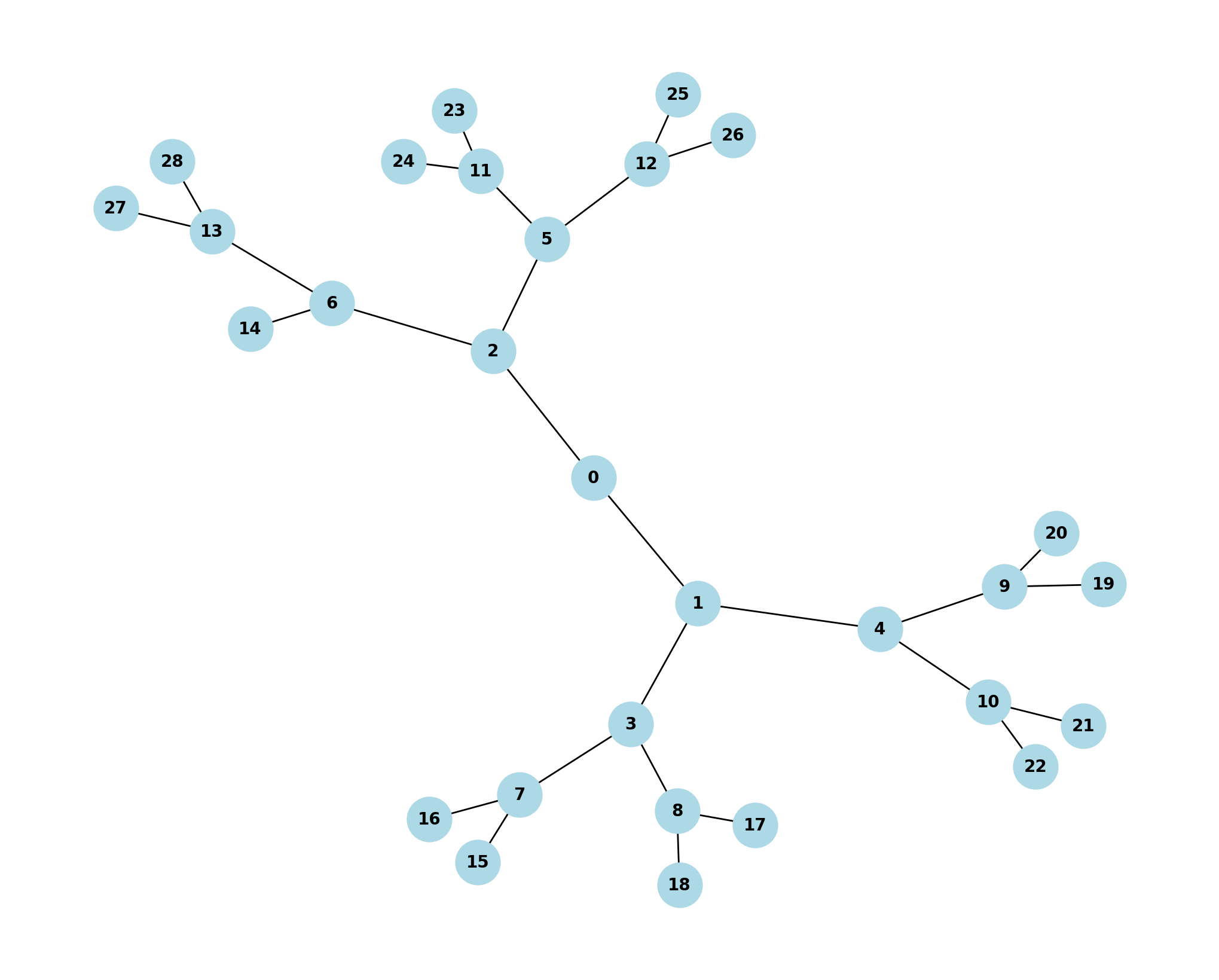
Figure 1: (Color Online) Binary Tree graph with 29 vertices and 28 edges, $G(29,28)$

We analyze a 29-vertex, 28-edge graph structured in a hierarchical, tree-like form, where the edges are grouped into 12 equivalence classes based on graph automorphisms. The goal is to determine the minimum number of trotterized layers, denoted $p$, required for the combined Reverse Causal Cone (RCC) to cover the entire graph.

At $p=1$, each RCC includes the qubits involved in a representative edge and their immediate neighbors, i.e., qubits one edge away. For example, the RCC for edge $(0,1)$ covers vertices $\{0,1,2,3,4\}$, while the RCC for edge $(0,2)$ covers vertices $\{0,1,2,5,6\}$. This approach is applied across all edge equivalence classes. At this layer, the combined RCC covers vertices $\{0,1,2,3,4,5,6,7,8,11,12,13,14,15,16,23,24,\\ 27,28,29\}$, leaving vertices $\{9,10,17,18,19,20,21,22,25,26\}$ uncovered. Therefore, $p=1$ is insufficient for complete coverage.

At $p=2$, RCCs expand to include qubits two edges away from the representative edge, capturing the previously uncovered vertices. For instance, the RCC for edge $(3,7)$, initially covering vertices $\{3,1,7,8,15,16\}$, now includes vertices $\{17,18\}$, which are neighbors of vertex 8. Similarly, the RCC for edge $(11,23)$, which initially covered vertices $\{11,5,23,24\}$, expands to include vertices $\{25,26\}$, neighbors of vertex 12. This expansion ensures complete graph coverage. Thus, a minimum of $p=2$ layers is required to fully cover the graph, as all vertices are included in the combined RCC structure at this level.

5.3 Automorphism-Assisted QAOA

Based on the discussions in the preceding sections, we propose a modification to the Quantum Approximate Optimization Algorithm (QAOA). In this modified approach, rather than measuring all the terms in the Hamiltonian, we restrict the measurements to a subset of terms selected using the graph automorphism group, Aut(G). The methodology for this approach is outlined as follows;

• Graph Definition: We begin by defining the graph $G=(V,E)$, where $V$ is the set of vertices and $E$ is the set of edges.

• Finding Edge Equivalence Classes Using Automorphisms: Next, we compute the automorphism group of graph $G$ to identify edge equivalence classes using the generators of the group1.

• Selecting a Representative Edge from Each Equivalence Class: From each edge equivalence class, we randomly choose one representative edge. This reduces the number of edges we need to consider, as we only focus on the representatives for the construction of the QUBO matrix.

• QUBO Matrix Initialization: After selecting the representative edges, we initialize a QUBO matrix of size $V\times V$, where $V$ is the number of vertices in the graph. This matrix will serve as a modified MaxCut formulation.

• Populating the QUBO Matrix: In this step, the QUBO matrix is populated. For each representative edge, the corresponding matrix element is assigned a non-zero value equal to the size of the equivalence class to which the edge belongs. All other matrix elements are set to zero. This modification of the standard MaxCut QUBO ensures that only the representative edges contribute to the optimization problem.

• Conversion to Ising Hamiltonian: The modified QUBO matrix is then converted into an Ising Hamiltonian using standard quadratic programming techniques. This Hamiltonian is optimized by the QAOA to approximate the solution to the MaxCut problem.

• QAOA Ansatz Construction: After constructing the modified Ising Hamiltonian, the QAOA ansatz is built using the original MaxCut Ising Hamiltonian, which includes all terms and edges. The QAOA ansatz involves alternating between two unitaries: one derived from the Ising Hamiltonian and another from a mixing Hamiltonian. The alternating sequence of these unitaries is parameterized by the angles $\gamma$ and $\beta$, which are optimized during the algorithm.

• Optimization: The final step involves optimizing the variational parameters $\gamma$ and $\beta$ to minimize the expectation value of the Ising Hamiltonian. While the QAOA ansatz is constructed from the full Hamiltonian, only terms in the modified Ising Hamiltonian are measured. The optimization is performed classically, and the result is an approximate solution to the MaxCut problem on the graph $G$.

• Obtaining the Optimal Solution: The optimized parameters $\gamma^{*},\beta^{*}$ are used to generate a final quantum state. By measuring this state, we obtain a bitstring that corresponds to the approximate solution of the MaxCut problem. This bitstring is the result of the QAOA process and represents the partition of the vertices of $G$ that maximizes the number of edges between the two partitions.

6 Results and Discussion

We employed the Quantum Approximate Optimization Algorithm with $p=1$ layer to solve MaxCut instances on tree-structured graphs, with node counts of up to 34. Two types of tree graphs were considered: binary trees and balanced trees, both generated using the NetworkX Python library. A key distinction between these graphs is that binary trees can exhibit uneven branch depths, particularly when the number of leaf nodes, $n$, is not a perfect power of two, resulting in an unbalanced structure. This asymmetry affects the number of edge equivalence classes in binary and balanced trees. The number of edge equivalence classes corresponds to a reduction in the number of terms in the Ising Hamiltonian, as outlined in Section 5.3. Tables 1 and 2 present the number of edge equivalence classes and the corresponding terms in the Ising Hamiltonian for MaxCut instances on binary and balanced trees, respectively. For comparison, we also provide the total number of terms in the full Hamiltonian, prior to any reductions.

G(V,E)	Edge Equiv. classes	$H_{reduced}$	$H_{full}$	Percentage Reduction
(5,6)	3	7	9	22.22%
(10,9)	7	15	19	21.05%
(15,14)	3	9	29	68.97%
(20,19)	11	24	39	38.15%
(25,24)	11	23	49	53.06%
(30,29)	13	30	59	49.15%
(31,30)	4	11	61	81.97%
(34,33)	16	35	67	47.76%

Table 1: Table for Binary Tree graph instances upto 34 vertices, depicting the number of edge equivalence classes, number of terms in reduced Hamiltonian $H_{reduced}$ and corresponding full problem Hamiltonian $H_{full}$, percentage reduction in terms

G(V,E)	Edge Equiv. classes	$H_{reduced}$	$H_{full}$	Percentage Reduction
(7,6)	2	5	13	61.54%
(13,12)	2	6	25	76%
(15,14)	3	7	29	75.86%
(31,30)	4	11	61	81.97%

Table 2: Table for Balanced Tree graph instances upto 31 vertices, depicting the number of edge equivalence classes, number of terms in reduced Hamiltonian $H_{reduced}$ and corresponding full problem Hamiltonian $H_{full}$, percentage reduction in terms

An upword trend in the Percentage Reduction of the number of terms in the Hamiltonian can be seen in Tables 1 and 2. Particularly for $G(15,14)$ and $G(31,30)$ binary trees, the reduction is high. For these graphs the vertex symmetry around root node results in a larger automorphism group as compared to their previous instances $G(10,9)$ and $G(30,29)$, respectively. For these graphs, all the vertices on the right of the root node can permute with those on the left without changing the graph structure. This leads to an increase in the number of equivalent edges belonging to same class. Consequently, the total number of edge equivalence classes decreases, thereby decreasing the complexity of the Ising Hamiltonian.

We conducted Python simulations on TPU-v2 cores, utilizing a system with 96 vCPUs and 350 GB of memory, provided through Google Colab. Although TPU acceleration for matrix multiplication was not utilized in this setup, the availability of a high number of vCPUs and substantial memory resources enabled the efficient execution of the simulations. The significance of this computational capacity is reflected in the results presented in Tables3 and 4. To compute the minimum eigenvalue, we employed the EstimatorV2 class from qiskit-ibm-runtime module with AerSimulator() as backend. The circuit gate rotation parameters, $\beta$ and $\gamma$, were optimized using the classical COBYLA optimizer. Figure 2 illustrates the optimizer-time required for each graph $G(V,E)$ in both binary and balanced tree structures to achieve the minimum eigenvalue.

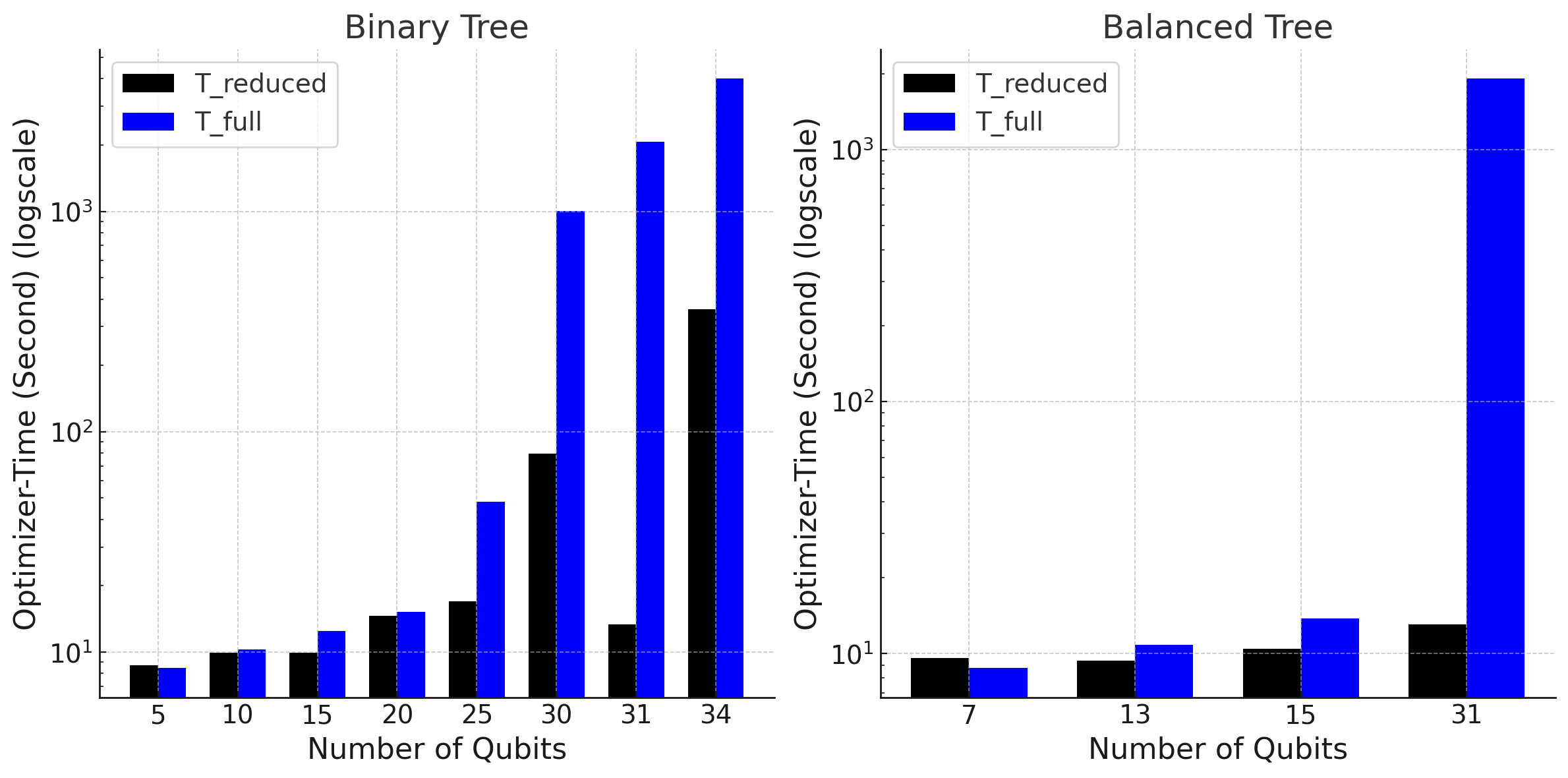
Figure 2: (Color Online) COBYLA optimizer-time bar plots for Binary and Balanced Tree graphs. Blue, Black bar denotes time taken for finding optimal parameters by measuring terms in full and reduced problem Hamiltonian respectively

Subsequently, we sampled the full quantum circuit using the optimal parameters obtained from the optimization process. The approximation ratios for the MaxCut problem were calculated for both the full Hamiltonian and the reduced Hamiltonian, with the latter leveraging graph automorphisms to reduce complexity. The approximation ratio $R$ here is defined as the ratio of the maximum value of the objective function obtained using QAOA ansatz to that obtained via a classical solver, such as CPLEX or GUROBI. For MaxCut instances on tree-structured graphs, where no cycles exist, the exact value of the objective function corresponds to the total number of edges in the graph. Tables 3 and 4 provide a detailed comparison of the optimizer-time, approximation ratio, and maximum system memory used for each instance.

G(V,E)	$T_{red}$(Sec)	$T_{full}$(Sec)	$R_{red}$	$R_{full}$	Peak Mem (Red) (GB)	Peak Mem (Full) (GB)
(5,4)	8.72	8.45	1	1	5.2	5.2
(10,9)	9.89	10.25	1	1	5.2	5.2
(15,14)	9.90	12.50	1	1	5.3	5.3
(20,19)	14.56	15.27	0.84	0.84	5.3	5.3
(25,24)	16.97	48.25	0.83	0.83	5.4	5.8
(30,29)	79.55	1004.32	0.76	0.76	6.4	21.5
(31,30)	13.34	2067.36	0.80	0.80	5.4	37.4
(34,33)	360.56	$>$3600	0.76	0.76	21.7	262.5

Table 3: Binary Tree Results

G(V,E)	$T_{red}$(Sec)	$T_{full}$(Sec)	$R_{red}$	$R_{full}$	Peak Mem (Red) (GB)	Peak Mem (Full) (GB)
(7,6)	9.63	8.75	1	1	5.2	5.2
(13,12)	9.38	10.82	1	1	5.2	5.2
(15,14)	10.44	13.78	0.93	0.93	5.2	5.3
(31,30)	13.02	1907.91	0.83	0.80	5.2	37.5

Table 4: Balanced Tree Results

The results presented in Tables 3 and 4 clearly highlight the computational advantages of utilizing reduced Hamiltonians in QAOA-based simulations for solving MaxCut on tree-structured graphs. One of the key findings is the significant reduction in optimizer-time when using the reduced Hamiltonian, particularly for larger graphs. While the performance difference between the reduced and full Hamiltonians is relatively minor for smaller graphs, it becomes increasingly pronounced as the size and complexity of the graph increase. Infact the optimizer-time using all the terms in the Hamiltonian for the 34 qubit MaxCut instance exceeded 3600 second as presented in Table 3 and we had to terminate it due to time restrictions on Colab. Compared to 360.56 second using the reduce Hamiltonian, this amounts to a reduction of more than $90\%$. In terms of memory consumption, the simulation using reduced Hamiltonian consistently requires less peak memory compared to the full Hamiltonian. This reduction becomes especially critical for large graphs, where memory constraints often limit the feasibility of quantum simulations. The reduced memory usage makes this approach more scalable and practical, particularly when dealing with resource-intensive computations on larger instances. Importantly, these efficiency gains are achieved without any compromise in solution quality. The approximation ratios, $R_{\text{red}}$ and $R_{\text{full}}$, are almost identical across all cases. This indicates that the use of reduced Hamiltonians at the least preserves the accuracy of the results. As with Table 1 we note here the computational time and resources for $G(15,14)$ and $G(31,30)$ for the binary tree case. At these instances the binary tree maps into a balanced tree. A balanced tree has more structural symmetry as discussed above. Here we we see how structural symmetry in graph plays an important role in significantly lowering optimizer-time and peak memory even though the number of qubits are more than the previous instances respectively.

It is important to highlight that in the simulations presented here, we consistently use $p=1$, representing only the first Trotterized layer, regardless of the graph size. This approach may appear to contradict the discussion in Section 5, where the combined Reverse Causal Cone (RCC) structure does not encompass all vertices at $p=1$ and hence does not include all two-qubit gates. For larger graphs, it may be necessary to increase $p$ beyond 1 to fully capture the RCC structure of all representative edges. However, based on the results in this section, it is evident that not all two-qubit gates are essential to determine the optimal gate parameters in QAOA. At $p=1$, the two-qubit gates that are not in the immediate neighborhood of the representative edges commute through, meaning they do not contribute to the optimization process. Consequently, as not all two-qubit gates are employed in the optimization, the computation time required by the optimizer is reduced, particularly for larger graphs. This speed-up, however, would be lost in cases where all two-qubit gates are incorporated into the RCC structure at $p=1$. An illustrative example is the star graph with $n$ vertices, where there exists only one edge equivalence class, as all vertices are symmetrically distributed around the central vertex. In this scenario, all vertices are in the immediate vicinity of the central vertex, and thus, regardless of the choice of representative edge, all two-qubit gates are included in the RCC structure. Hence there would not be a particular difference in performance using AA-QAOA or vanilla QAOA. Table 5 presents a comparison of optimizer times for star graphs with 28 and 29 vertices, further illustrating this effect.

G(V,E)	$T_{red}$(Sec)	$T_{full}$(Sec)	$R_{red}$	$R_{full}$
(28,27)	79.16	83.94	0.963	1
(29,28)	187.26	190.16	0.964	0.964

Table 5: Table depicting optimizer-time for star-structured graph with 28 and 29 vertices.

The optimizer-time for $G(28,27)$ and $G(29,28)$ are similar for both full and reduced Hamiltonians, as seen from Table5. This shows no improvement in efficiency eventhough the number of terms in the reduced Hamiltonian are far less than those in the full Hamiltonian. As mentioned above, this discrepancy can be attributed to the fact that all the two-qubit gates are included in the RCC structure of the representative edge/s at $p=1$.

7 Conclusion

In this work, we have demonstrated that leveraging graph automorphisms to reduce the number of terms in the problem Hamiltonian for the Quantum Approximate Optimization Algorithm (QAOA) is a promising and effective strategy for solving graph optimization problems. We introduced AA-QAOA, a modification of the standard QAOA, and applied it to the unweighted MaxCut problem as a representative example. By exploiting the symmetries inherent in graph automorphisms, we significantly reduce the number of Hamiltonian terms, thereby reducing computational complexity while maintaining the quality of the solutions.

Our results further indicate that the optimal gate rotation parameters can be efficiently determined using two-qubit gates at $p=1$, derived from the Reverse Causal Cone (RCC) structure of the terms in the reduced Hamiltonian. Specifically, for tree-structured graphs, only the two-qubit gates corresponding to edges between nearest neighbors of the measured qubits are involved for a single Trotterized layer. This eliminates the necessity of computing the entire RCC structure for the measured qubits, which contrasts with prior approaches where the complete RCC structure was integral to the optimization process. The selective inclusion of these gates is the key to the computational speedup observed in our results. It is also worth mentioning that in some cases, only reducing the number of terms in the Ising Hamiltonian is not a sufficient condition to observe an increase in computational efficiency, as indicated by the implementation of our analysis to star-structured graphs. It is important to check whether all two-qubit gates(graph edges) are included in the RCC structure of the representative edge at $p=1$, in which case there would be no significant increase in computational efficiency.

Although this analysis is presently restricted to tree-structured graphs, it suggests that the approach is both scalable and robust, making it a valuable method for quantum optimization. The insights gained from this work highlight the potential of symmetry-based reductions in quantum algorithms and open up avenues for extending these techniques to higher number of qubits and directly solving them on a quantum hardware. Also given the current limitation to tree-structured graphs, it is crucial to explore the extension of our method to more complex graph structures.

References

- [1] Edward Farhi, Jeffrey Goldstone, and Sam Gutmann. A quantum approximate optimization algorithm, 2014.
- [2] Linghua Zhu, Ho Lun Tang, George S. Barron, F. A. Calderon-Vargas, Nicholas J. Mayhall, Edwin Barnes, and Sophia E. Economou. Adaptive quantum approximate optimization algorithm for solving combinatorial problems on a quantum computer. Phys. Rev. Res., 4:033029, Jul 2022.
- [3] Yahui Chai, Yong-Jian Han, Yu-Chun Wu, Ye Li, Menghan Dou, and Guo-Ping Guo. Shortcuts to the quantum approximate optimization algorithm. Phys. Rev. A, 105:042415, Apr 2022.
- [4] Zeqiao Zhou, Yuxuan Du, Xinmei Tian, and Dacheng Tao. Qaoa-in-qaoa: Solving large-scale maxcut problems on small quantum machines. Phys. Rev. Appl., 19:024027, Feb 2023.
- [5] Takuya Yoshioka, Keita Sasada, Yuichiro Nakano, and Keisuke Fujii. Fermionic quantum approximate optimization algorithm. Phys. Rev. Res., 5:023071, May 2023.
- [6] Johannes Weidenfeller, Lucia C. Valor, Julien Gacon, Caroline Tornow, Luciano Bello, Stefan Woerner, and Daniel J. Egger. Scaling of the quantum approximate optimization algorithm on superconducting qubit based hardware. Quantum, 6:870, December 2022.
- [7] Aditi Misra-Spieldenner, Tim Bode, Peter K. Schuhmacher, Tobias Stollenwerk, Dmitry Bagrets, and Frank K. Wilhelm. Mean-field approximate optimization algorithm. PRX Quantum, 4:030335, Sep 2023.
- [8] Reuben Tate, Jai Moondra, Bryan Gard, Greg Mohler, and Swati Gupta. Warm-Started QAOA with Custom Mixers Provably Converges and Computationally Beats Goemans-Williamson’s Max-Cut at Low Circuit Depths. Quantum, 7:1121, September 2023.
- [9] Stefan H. Sack, Raimel A. Medina, Richard Kueng, and Maksym Serbyn. Recursive greedy initialization of the quantum approximate optimization algorithm with guaranteed improvement. Phys. Rev. A, 107:062404, Jun 2023.
- [10] Shaydulin Ruslan, Stuart Hadfield, Tad Hogg, and Ilya Safro. Classical symmetries and the quantum approximate optimization algorithm. Quantum Information Processing, 20:1573–1332, 2021.
- [11] Sergey Bravyi, Alexander Kliesch, Robert Koenig, and Eugene Tang. Obstacles to variational quantum optimization from symmetry protection. Phys. Rev. Lett., 125:260505, Dec 2020.
- [12] Soumalya Joardar and Arnab Mandal. Quantum symmetry of graph c∗-algebras associated with connected graphs. Infinite Dimensional Analysis, Quantum Probability and Related Topics, 21(03):1850019, 2018.
- [13] Leonardo Lavagna, Simone Piperno, Andrea Ceschini, and Massimo Panella. On the effects of small graph perturbations in the maxcut problem by qaoa, 2024.
- [14] Zhenyu Cai. Quantum Error Mitigation using Symmetry Expansion. Quantum, 5:548, September 2021.
- [15] Ruslan Shaydulin and Stefan M. Wild. Exploiting symmetry reduces the cost of training qaoa. IEEE Transactions on Quantum Engineering, 2:1–9, 2021.
- [16] Brendan D. McKay and Adolfo Piperno. Practical graph isomorphism, ii. Journal of Symbolic Computation, 60:94–112, 2014.
- [17] Jules Tilly, Hongxiang Chen, Shuxiang Cao, Dario Picozzi, Kanav Setia, Ying Li, Edward Grant, Leonard Wossnig, Ivan Rungger, George H. Booth, and Jonathan Tennyson. The variational quantum eigensolver: A review of methods and best practices. Physics Reports, 986:1–128, 2022.