[][nocite]supp
Model-free Estimation of Latent Structure via
Multiscale Nonparametric Maximum Likelihood
Abstract
Multivariate distributions often carry latent structures that are difficult to identify and estimate, and which better reflect the data generating mechanism than extrinsic structures exhibited simply by the raw data. In this paper, we propose a model-free approach for estimating such latent structures whenever they are present, without assuming they exist a priori. Given an arbitrary density , we construct a multiscale representation of the density and propose data-driven methods for selecting representative models that capture meaningful discrete structure. Our approach uses a nonparametric maximum likelihood estimator to estimate the latent structure at different scales and we further characterize their asymptotic limits. By carrying out such a multiscale analysis, we obtain coarse-to-fine structures inherent in the original distribution, which are integrated via a model selection procedure to yield an interpretable discrete representation of it. As an application, we design a clustering algorithm based on the proposed procedure and demonstrate its effectiveness in capturing a wide range of latent structures.
Introduction
Multivariate distributions are known to possess exotic structures in high-dimensions, which makes density estimation difficult in higher and higher dimensions. At the same time, multivariate distributions often possess intrinsic structure that can be easier to capture compared to say, estimating the entire density at fine scales. There are many known examples of this phenomenon: discrete structure in the form of clustering or mixtures (Wolfe, 1970, McLachlan and Chang, 2004, Stahl and Sallis, 2012), low-dimensional structure in the form of a manifold (Belkin et al., 2006, Lin and Zha, 2008) or sparsity (Hastie et al., 2015), dependence structure in the form of a graph (Banerjee and Ghosal, 2015, Lee and Hastie, 2015, Drton and Maathuis, 2017), or functional restrictions such as convexity (Bartlett et al., 2006), monotonicity (Ramsay, 1998), and hierarchical or compositional structure (Juditsky et al., 2009). In the literature on nonparametric estimation, it is now well-known that low-dimensional structures (i.e. functionals) can be captured much more efficiently than the entire density.
Motivated by these observations, in this paper we revisit a simple question from a new perspective: To what extent can discrete structures be identified and estimated in general, high-dimensional densities, without necessarily assuming an analytic form of such a structure a priori? In other words, is there a natural model-free notion of discrete structure that is statistically meaningful and estimable for arbitrary densities?
We propose such a recipe for deciphering latent structures inherent in an arbitrary density that leads to practical algorithms. We do not impose any restrictions on the form of ; in particular, we do not assume any mixture, clustering, or latent class structure to begin with. Our approach starts by treating and estimating the latent structure of as a nonparametric parameter, taking the form of a latent probability measure. This measure, computed via nonparametric maximum likelihood estimation (NPMLE, Kiefer and Wolfowitz, 1956), to be introduced shortly, can be interpreted as a compressed representation of or samples from it. The crucial feature of this latent measure is that its support carries a rich geometry with a clearer structure than the original density . A refined analysis on the support then reveals the hidden structures of . The key aspect of our approach lies in how we construct this latent measure and its support, and its reliance on a hyperparameter that controls the scale of the representation. In particular, by computing this across a range of ’s, we reveal coarse-to-fine, “multi-scale” structures of , which can be integrated to yield a most representative model that is useful for various downstream tasks. As an example application, we will illustrate its use for clustering tasks.
Overview
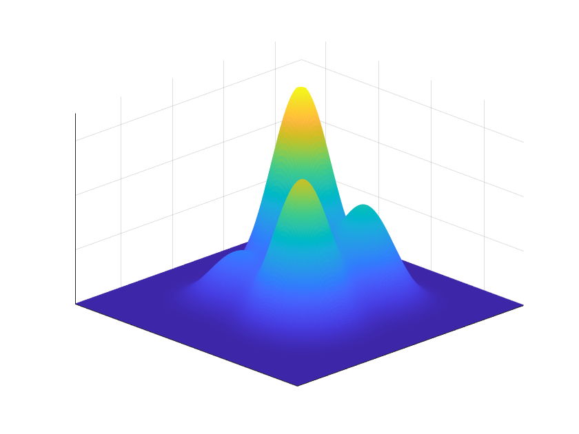
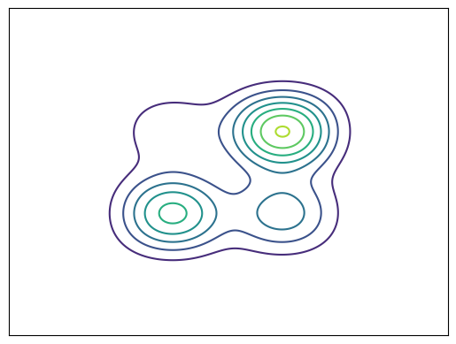
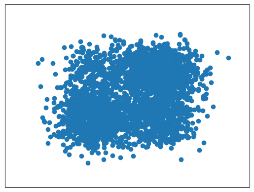
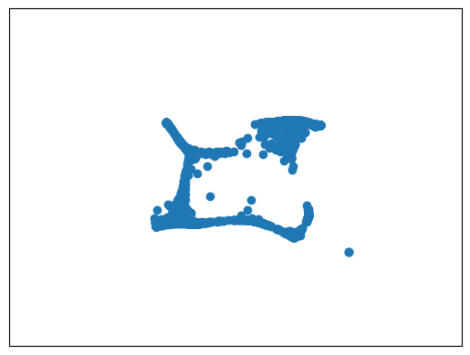
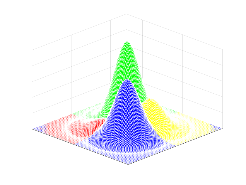
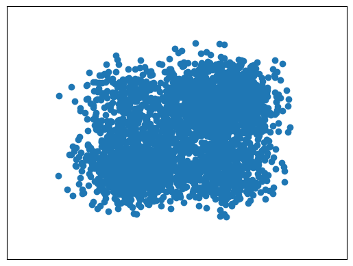
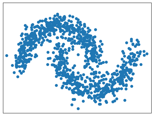
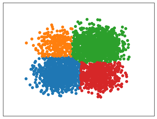
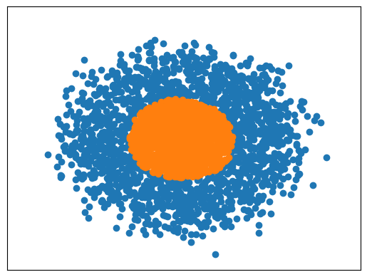
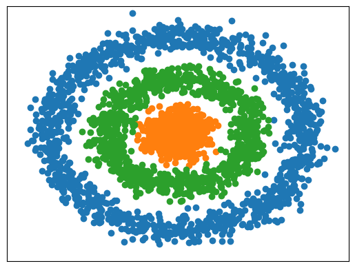
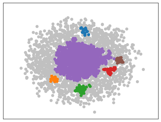
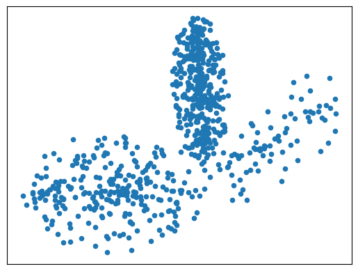
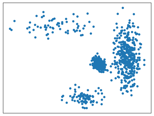
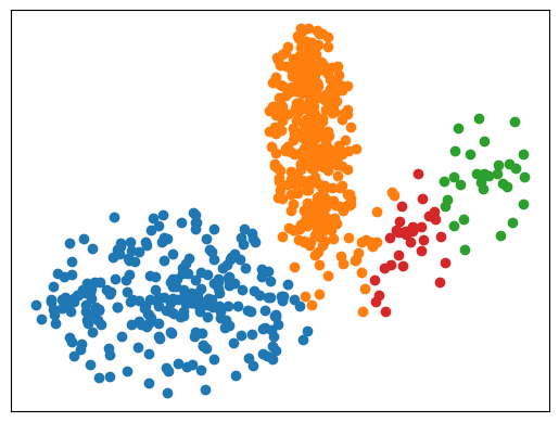
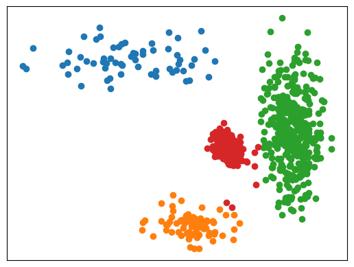
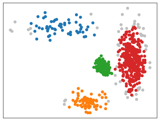
To gain some intuition on what this latent structure looks like, we first present the main ideas at a high-level, deferring technical details to Sections 2-3. Consider the two-dimensional example shown in Figure 1, which displays the density map, its contour plot, and a scatter plot of samples generated from it. This simulated nonparametric density has four modes with different heights that are not very well separated, and which do not form meaningful clusters that can be discerned from the raw data. The latent structure, captured by the aforementioned latent measures and computed via the NPMLE, is pictured in Figure 2. This shows the supports of different latent measures for several increasing values of , which are seen to exhibit very different structures. In particular, it transitions from a densely supported measure () to a sparse one (). One can interpret such dynamics as the merging and separation of a collection of points representing the latent structures at different scales.
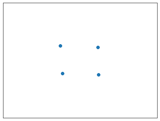
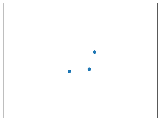
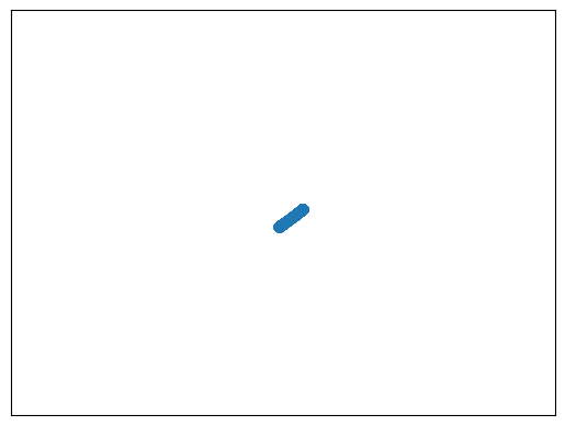
For each value of the hyperparameter , the latent measures in Figure 2 capture the intrinsic discrete structure of at different scales that we call a multiscale representation of . This is reminiscent of the bias-variance tradeoff in density estimation (e.g. in choosing the bandwidth or number of neighbours), however, our target is quite different: Instead of recovering the density , we aim to recover discrete structure such as intrinsic clusters or mixture components—without assuming their existence a priori. If density estimation were our goal, then choosing or even smaller in Figure 2 would be preferable, but clearly this measure does not capture the four clusters in in any meaningful way.
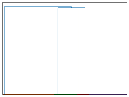
After constructing the multiscale representation of , the next step is to select a choice of that best captures this discrete structure. We will propose a model selection procedure that returns the third measure with (Figure 2)—indicated by —as the selected model in this example, which contains precisely four clusters of atoms representing the four high density regions of the original density . Moreover, this latent structure will be captured much more concretely and rigourously than simply inspecting the support of by eye. The measure in fact defines several objects that are useful:
-
1.
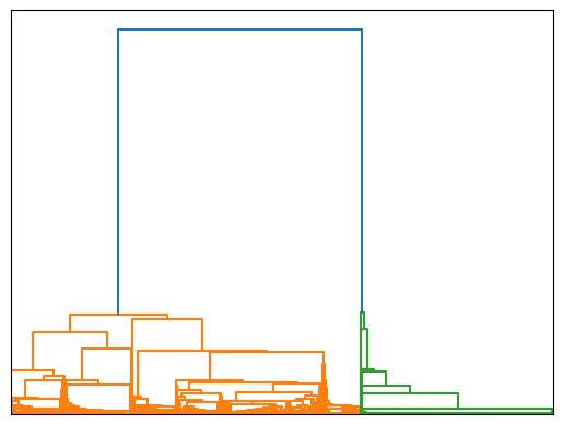
defines a dendrogram, which provides a more nuanced and qualitative view of the latent geometry. This for instance serves to help infer an approximate number of discrete states or latent classes. See Figure 3.
-
2.
We can also use to define estimates of class conditional densities over each cluster, as in Figure 3.
-
3.
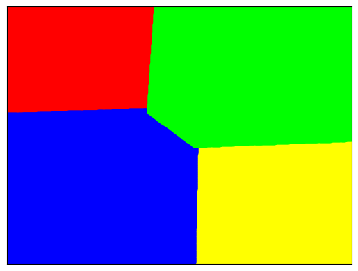
We can use to define a partition of the input space as in Figure 3, and thus also a clustering of the original input data points.
Thus, not only captures a quantitative notion of structure, to be introduced in the sequel, but also useful qualitative notions of structure that can be used for model assessment and validation.
Crucially, this example makes no assumptions on the form of , and applies to any density. It appears as though the measure is capturing the intrinsic, discrete structure of without exploiting specific parametric or structural assumptions on it. While intuitively appealing, making this precise requires some effort. Moreover, there are several practical challenges to tackle including computation, high-dimensionality, and the selection of . Below we shall briefly introduce the main tools of our approach, followed by a summary of our results and contributions.
Main Ingredients
A central tool that we shall employ in this paper for computing the probability measure is the nonparametric maximum likelihood estimator (NPMLE, Kiefer and Wolfowitz, 1956). Formally speaking, this is an estimator defined as
| (1) |
where are samples from and is a suitable space of probability densities to be defined shortly. Instead of a finite-dimensional parameter space as in the usual maximum likelihood estimation, (1) searches over a potentially infinite-dimensional space. Due to its nonparametric nature, some care is needed in specifying the search space . For example, if we naïvely choose the space of all continuous densities , we can see that the objective function value in (1) would tend to infinity on a sequence of densities approximating the empirical measure .
The issue lies in the overly large parameter space which allows to be arbitrarily narrow and spiked. Therefore to make the problem well-posed, we shall restrict our attention to the set of all densities with a “minimum length-scale” . This is achieved by considering densities of the form for some kernel with bandwidth , with ranging through the set of all probability measures. Denoting this collection of such densities as , we can see that the maximization (1) over would equivalently give a probability measure , which we hope captures some of the latent structure in the original density . More formally, can and will be interpreted as a latent projection of onto that removes spurious effects from the data and retains only the latent structure.
This then brings up the key aspect of our approach, namely the idea of multiscale representation. More precisely, by computing the NPMLE (1) across a range of ’s, we reveal latent structures of at different scales as we have seen in Figure 2. In particular, as , the density becomes more and more expressive by drawing analogy with kernel density estimators (i.e. interpreting as encoding all the centers). It is therefore more likely to find an element that fits the original density well so that as well as the associated measure both inherit the fine scale structures of . On the other hand, as becomes larger, the kernel becomes flatter so that the stronger projection effect would render a sparse structure in . As in Figures 1-2, the support of in this regime can inform us about the coarse scale information of such as the number and location of the high density regions. As we shall demonstrate later, the structures obtained across different ’s can be leveraged to select ideal models that best represent .
Summary of Results and Contributions
The main contribution in this paper is a novel recipe for identifying and estimating the latent structure of general densities based on the idea of multiscale analysis introduced above, which is made practical via the NPMLE. We shall present results on both theoretical and practical aspects.
On the theory side, we first give a characterization of the asymptotic limit of the NPMLE as a certain projection of the original density . We then proceed to study the discrete structures in by identifying them with a notion of components from the perspective of mixture models. We propose an estimation procedure for these components based on the NPMLE and establish its consistency. These results justify our approach for estimating the latent structures of general densities that enjoys a valid mathematical interpretation, and which provides foundations for downstream applications such as cluster analysis.
On the practical side, we propose a model selection procedure for finding a “most sparse model” from the multiscale representation that explains the data well and turn this into a clustering algorithm. Moreover, the model selection rule gives a natural estimate of the number of clusters so the algorithm is essentially tuning-free, although a pre-specified number can also be fed into the algorithm. We demonstrate through numerical experiments that our algorithm is able to resolve a wider range of complex latent structures than standard ones such as -means, spectral clustering and HDBSCAN.
Related Work
A closely related line of work is cluster analysis, where two major approaches are density-based clustering and model-based clustering. Our work shares many common features with both despite being intrinsically different. In density-based clustering, one is often either interested in estimating the connected components of the level sets (Hartigan, 1981, Ester et al., 1996, Steinwart, 2011, Sriperumbudur and Steinwart, 2012, Steinwart, 2015, Jang and Jiang, 2019) or the cluster tree of the density (Chaudhuri and Dasgupta, 2010, Stuetzle and Nugent, 2010, Chaudhuri et al., 2014). The (empirical) level sets are similar to the NPMLE as both tend to capture high density regions of the original density . However, the NPMLE is defined through a more involved optimization scheme and appears to give a more sparse summary of the high density regions as can be seen from Figure 2, where only a few clusters of points are visually present for . A conceptually similar algorithm is the hierarchical DBSCAN (Campello et al., 2013) which performs DBSCAN (Ester et al., 1996) for range of connectivities ’s and returns a clustering with the best stability over . The algorithm searches for clustering structures on high density regions of the data samples whereas our approach works with the NPMLEs instead, and are not necessarily supported on subsets of the data points. On the other hand, the sequence of NPMLEs computed for different ’s is reminiscent of the cluster tree. However, we point out that the nodes of a cluster tree are nested sets whereas the support atoms of are not. Furthermore, the overall trend for the NPMLE may not even be monotone with respect to as can be seen from Figure 2.
In model-based clustering, one typically assumes the existence of a mixture decomposition and attempts to identify and estimate it. There is a vast literature on model-based clustering (Fraley and Raftery, 2002) and here we shall refer to the review papers Melnykov and Maitra (2010), McNicholas (2016) and the references therein. In the recent work Coretto and Hennig (2023), the authors consider maximum likelihood estimation of mixtures of elliptically symmetric distributions and apply such models for fitting general nonparametric mixtures. Another recent work is Do et al. (2024), where the authors first estimate an overfitted mixture model, followed by a refinement process based on a dendrogram of the estimated parameters. However, we mention that the authors still assume the data to be generated by a finite mixture model and focus only on parametric cases. A major difference between our approach and model-based clustering is that there is no assumed model for but rather a sequence of proxies defined by the NPMLEs, employed only for the purpose of extracting structural information from . In other words, we do not necessarily expect that any of the surrogate models matches the truth, but only use them as tools for identifying and estimating the latent structures of .
Another closely related line of work is the study of nonparametric mixture models, which play a role in our technical development. Instead of specifying an explicit form of the mixture components, the nonparametric approach imposes structural assumptions on the component densities such as symmetry (Bordes et al., 2006, Hunter et al., 2007), latent structures (Allman et al., 2009, Gassiat and Rousseau, 2016), product structures (Hall and Zhou, 2003, Hall et al., 2005, Elmore et al., 2005), and separation (Aragam et al., 2020, Aragam and Yang, 2023, Tai and Aragam, 2023). Related results on the identifiability and estimation of nonparametric mixtures can also be found in Nguyen (2013). A recent Bayesian clustering approach is proposed in Dombowsky and Dunson (2023) by merging an overfitted mixture under a novel loss function, which is shown to mitigate the effects of model misspecification. The idea of merging overfitted mixtures has recently generated some attention (e.g. Aragam et al., 2020, Guha et al., 2021, Aragam and Yang, 2023, Dombowsky and Dunson, 2023, Do et al., 2024). We emphasize that unlike this line of work, we do not assume a mixture representation for the data generating mechanism.
Finally, we return to the key technical device employed, namely the NPMLE, which has attracted increasing attention over the past decades. One of the earlier uses of the NPMLE lies in estimating the mixing measures of mixture models (Lindsay, 1995) and finding superclusters in a galaxy (Roeder, 1990). In a recent line of work, several authors have continued this endeavor with a focus on establishing convergence rates for density estimation (Genovese and Wasserman, 2000, Ghosal and Van Der Vaart, 2001, Zhang, 2009, Saha and Guntuboyina, 2020), and its application in Gaussian denoising (Saha and Guntuboyina, 2020, Soloff et al., 2024). Apart from the various applications, the NPMLE is itself a mathematically intriguing estimator that carries interesting geometric structures (Lindsay, 1983a, b). In particular, it can be shown that the NPMLE is a discrete measure supported on at most atoms where is the number of observations (Soloff et al., 2024). The recent work Polyanskiy and Wu (2020) has improved this bound to for one-dimensional Gaussian mixtures with a sub-Gaussian mixing measure, matching the conventional wisdom that usually many fewer support atoms are present. Our empirical observation (such as those in Figure 1) also suggests a tendency for the NPMLE to be supported only on a few atoms when is large. In Proposition 2.4 we establish an upper bound in terms of . Lastly, although the NPMLE is computationally intractable as it is posed as an infinite-dimensional optimization problem, much progress has also been witnessed on computational aspects of the NPMLE, including a convex approximation (Feng and Dicker, 2018) and gradient flow-based methods (Yan et al., 2024, Yao et al., 2024), making it practical for high-dimensional problems.
Notation
For a set , we shall denote the set of all probability measures supported on . For a function and a probability measure over , we denote as the convolution of with . We also denote
| (2) |
For two subsets , we denote . If is a singleton, we shall simply denote as . For , we denote . For , the -Wasserstein distance for is defined as
| (3) |
where is the set of couplings between and .
The rest of the paper is organized as follows. In Section 2, we formalize our setting and present preliminary results that serve as foundations for later development. In Section 3, we present our main results on identifying and estimating the latent structures of general densities. Section 4 describes a clustering algorithm that arises from an application of our estimation procedure, followed by numerical experiments in Section 5. All proofs are deferred to the Appendix.
Preliminary Results
In this section we shall formalize our setting by making precise the various concepts mentioned above. We shall present preliminary results on the characterization of the asymptotic limit of the NPMLE and discuss its interesting geometric structure in the context of the multiscale analysis. To start with, we shall introduce an important family of densities, alluded above as the set of densities with minimum length-scale , which will play a crucial role in our later development.
Here and throughout the rest of the paper, the density that generates our data is allowed to be arbitrary: We will not need to impose any further regularity conditions on besides the fact that it is a density. In fact, a major contribution of our framework is to define—for any —an appropriate multiscale latent representation () that will be the target of estimation.
Convolutional Gaussian Mixtures
We begin by formalizing the family of probability measures used in the sequel for defining the NPMLE. Consider the family of convolutional Gaussian mixtures, defined as
| (4) |
where is the probability density function of the multivariate Gaussian , and is the set of all probability measures supported on . Densities in can be interpreted as a continuous mixture of Gaussians , where the center ’s are encoded in the mixing measure . The set includes finite Gaussian mixtures as a special case when the mixing measure is a sum of Dirac delta functions. As varies over , (4) forms a rich nonparametric family of densities with controlling their latent structures. Furthermore, given any the underlying mixing measure is identifiable so that its estimation is a well-posed statistical question.
Nonparametric Maximum Likelihood Estimator
Now that we have defined the space of candidate densities, we are ready to make precise our definition of NPMLE. Let be i.i.d. samples from . For , define
Since densities in are of the form for with being identifiable, the above maximization can be equivalently cast as
| (5) |
where we take any maximizer if there are multiple. As mentioned in the introduction, the measure will be the parameter of interest and for this reason we shall work with the definition (5) for the rest of the paper.
A natural question that follows is whether the NPMLE defined (5) has a valid asymptotic limit as . Thanks to the connection between maximum likelihood estimation and Kullback-Leibler (KL) divergence, it turns out that there is a nice interpretation of as approximating the KL projection of onto the space . To make this connection precise, let’s define
| (6) |
In other words, is the density in that is closest to in KL-divergence. Notice that the KL-divergence between and any element is always well-defined since the later is non-vanishing. The following result validates our definition of .
Proposition 2.1.
Let be a compact set and be any density. Then there exists a unique that solves (6).
Proof.
The proof can be found in Appendix A. ∎
With this definition, we can now state the following result, which generalizes Kiefer and Wolfowitz (1956) to arbitrary .
Proposition 2.2.
Proof.
The proof can be found in Appendix B. ∎
Remark 2.3.
In particular, Proposition 2.2 confirms the fact that is a consistent estimator of the mixing measure of the projection in distance. The result then suggests that in the asymptotic regime, the NPMLE resembles the projection so that they should share similar structures. For this reason, we shall base our discussion below on either the NPMLE or interchangeably since sometimes the population limit could yield more insights without the distraction of finite sample effects.
Geometry of NPMLE
It has been shown in the literature (Soloff et al., 2024, Lemma 1) that defined in (5) is a discrete measure supported only on at most atoms despite the search space being the space of all probability measures on . A crucial observation that will lead to the idea of multiscale analysis is that the NPMLE could exhibit very different structures for different choices of ’s. In particular, as increases, the number of support atoms present in tends to decrease and concentrate towards the high density regions of . This can be already seen in Figure 2. The following result then makes this rigorous in the one-dimensional case.
Proposition 2.4.
Suppose and the ’s are ordered increasingly. Define . We have
| (7) |
If , is a Dirac delta measure located at the mean .
Proof.
The proof can be found in Section C. ∎
Notice that the right hand side of (7) is a decreasing function of and if exceeds certain threshold, only one flat Gaussian remains. However, the result does not imply that the number of atoms in decreases monotonically with respect to , but only an overall decreasing trend as can be seen also in Figure 2. A typical observation is that if has well-separated modes, then for certain ranges of ’s will have (close to) atoms located around these modes. If one keeps increasing , those atoms will merge further but many more atoms could be present during such transition. A more refined characterization of the atom locations in is an interesting theoretical question to be investigated in the future. Theoretical analysis of NPMLE is still emerging and we mention the recent works Polyanskiy and Wu (2020), which gives an upper bound on the number of support atoms for a one-dimensional sub-Gaussian model and Soloff et al. (2024), Yan et al. (2024) which establish the existence of the NPMLE in general dimensions. Evidently, even basic questions about the NPMLE remain unresolved.
Remark 2.5.
We end this section by pointing out a qualitative difference between the NPMLE and its limit , namely that is always a discrete measure regardless of whether its limit is continuous or not (Soloff et al., 2024, Lemma 1). Therefore, the geometric structures in and should be analyzed using different approaches as for instance the notion of connected components in the support of does not immediately make sense. We shall address this issue in more detail in Section 4.
Multiscale Representation
With such preparation, we are now ready to make precise the idea of multiscale analysis. Following Remark 2.3, we shall focus the discussion below on the projections ’s. By definition of , we can write for some . Intuitively, we can view as a kernel density estimator with bandwidth , with containing possibly infinitely many centers. The choice of determines the width of the Gaussians used to approximate and affects the structure of the surrogate . The central idea underlying the multiscale representation is that for different choices of ’s, the measures ’s will exhibit structures of at different scales, which we illustrate next.
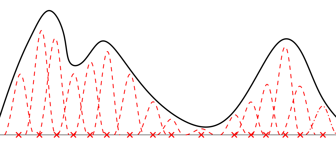
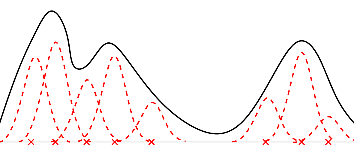
For general compact , as , becomes more expressive and its distance to decreases so that gives a better and better approximation to . In this case, the associated measure tends to be “dense”, meaning that substantially many Gaussians whose centers lie close to each other are needed for fitting due to the small bandwidth . On the other hand, as gets larger, flatter Gaussians are used instead to approximate , in which case one expects only a few of them to be present in . The underlying mixing measure then tends to be “sparse” and have smaller support sizes compared to the case of small ’s. Figure 4 gives a visualization for such an observation. In the extreme case of , the projection will approximate a single flat Gaussian centered at the mean of (cf. Proposition 2.4).
Of particular interest is the intermediate regime where is moderately large. In this case, the projection still gives a reasonable approximation to , while at the same time yields a sparse mixing measure whose atoms are centered near the high density regions of . Due to sparsity, the atoms are likely to be well-separated and a simple clustering of them would allow us to extract the number and locations of the different high densities regions of . This is precisely the type of structures captured by Figure 2 in the motivating example. In the next section, we shall discuss how to identify and estimate the finer structures within each of the ’s or their empirical counterparts ’s.
Estimation of Latent Structures
With these preliminaries out of the way, we now continue to discuss estimation of the latent structure as represented by the multiscale representation . Our goal is to use this representation to construct a well-defined notion of latent structure for across multiple scales , and then to give a procedure for estimating this latent structure. The resulting structure will be represented by a latent mixing measure for that approximately captures the structure in . The main result of this section (Theorem 3.5) will then construct strongly consistent estimators of this multiscale structure.
As before, let’s start the discussion from the projections by defining a notion of components for the projections as representing the latent structures of and then propose an estimation procedure for recovering them.
Components of the Projections
We are especially interested in the case where appears to be loosely comprised of multiple subpopulations, or unobserved latent classes, but for which we lack identifying assumptions such as Gaussianity for these classes. Another perspective is that has several high density regions that we wish to distinguish. See Figure 1. Bearing this intuition in mind, we will not assume such a structure explicitly exists, and instead will use the latent projections to locate approximations to this latent structure, and to analyze them from a mixture modeling perspective by viewing them as components of . Intuitively, the latent mixing measure should inherit such a mixture structure to some degree and therefore a natural target would be to estimate the components of , with the hope of them revealing the components of the original density . However, since is defined via the projection (6) and has no mixture structure a priori, the notion of components in remains unclear and undefined. One could imagine simply breaking down via the connected components of its support, but this could result in splitting up genuine clusters in : indeed, is only a proxy for , and so some care must be taken to extract information about from . Here we make this notion more explicit and quantitative.
We begin with the following preliminary decomposition of :
Definition 3.1.
Here, is the closure of the support of , which is also the smallest closed set such that . If has a density , then this is simply the closure of the set . The definition also includes the case where the support of is a lower-dimensional set in .
Definition 3.1 decomposes into a mixture of components, where each is simply the restriction of onto its -th connected component . Since these connected components are closed, the ’s are a collection of compactly supported probability measures whose supports must be separated by a positive distance:
where we recall the set-wise distance defined in Section 1.5. The geometry of the support of plays a crucial role in our construction and for different ’s, the decomposition can look very different with different numbers of components .
The decomposition (8) serves as a baseline for identifying the geometric structure of the support of , however, as discussed above it may not correctly capture the “right” structure in . For example, it is often natural to further group the ’s to merge nearby, fine structures that participate in the same grouping or cluster. For instance, if is a mixture of two components with each component being multi-modal, then for a certain range of ’s the decomposition (8) would exhibit many components, which should indeed be interpreted as a mixture of two components by grouping close components as a single one. Figure 5 gives such a visualization. In general, we can carry out such grouping until components are retained for any . The procedure amounts to applying single-linkage clustering on the supports ’s (as sets) until clusters remain, by repeatedly merging the closest components into one, which allows one to recover high-level discrete structures of .

Definition 3.2.
For , let be the collection of sets obtained from applying single-linkage clustering to until sets are retained.
With this definition, we can write down a similar decomposition as in (3.1):
| (9) |
By defining the corresponding component densities , it follows that
| (10) |
Moreover, we have the separation condition
| (11) |
Although the support of each may no longer be connected, this definition guarantees that the distance between any and for is larger than the pairwise distances between any two connected components inside the ’s.
As with the scale , the number of components is not a part of the underlying model, which is simply an arbitrary density . Thus, we cannot ask to identify or estimate the “right” . At the same time, the choice of here is crucial since it will then define the components that one wishes to identify and estimate, which can be very different across different values of . Nevertheless, the decomposition (9) and the estimation procedure that we shall describe below holds for any value of , and estimates potentially different underlying structures of corresponding to a specific . In Section 4, we shall propose an empirical approach to select a good candidate for based on the multiscale representation of and the resulting dendrogram (Figure 3) that our procedure returns. Alternatively, the choice of may come from one’s prior knowledge on the data generating mechanism, including the number of heterogeneous groups known in the dataset or the number of modes observed. We defer additional discussion on this point to Section 4.
Finally, it is worth contrasting (8) and (9): (8) is an uninformative decomposition of into connected components, whereas (9) refines this decomposition into a coarse-grained decomposition into informative clusters that we wish to estimate. Thus, in the sequel, our target of estimation shall be as defined in (9).
Estimating the Components
With the decomposition (9)-(10) in mind, we shall now focus on estimating the weights ’s and the densities . The procedure is almost ready as Proposition 2.2 suggests that is a consistent estimator of so that asymptotically it should also satisfy a discrete version of (3.1), where the support atoms of have “connected components” that are separated by a positive distance as in (11). However, since is always a discrete measure, this intuition is not precise, and we must be careful when comparing the decomposition of the continuous measure with its discrete approximation ; recall Remark 2.5.
Fortunately, we expect the discrete atoms of to be densely packed so that there are only tiny “holes” within each component of . In particular, by applying single-linkage clustering on these discrete atoms until clusters remain, we expect to obtain the correct cluster assignments of the atoms and hence good approximations of the supports ’s. We remark that this intuition is often correct in practice, especially with moderately larges ’s where the separation is much stronger than (11). Examples include those in Figures 8 and 12 where we can see clearly a clustering structure. However, from a theoretical perspective, the convergence established in Proposition 2.2 does not directly imply this kind of “nice” structure: There are many more possibilities for the configurations of the atoms in that are consistent with convergence. In particular, there could be atoms with vanishingly small weights lying in between the different components so that the separation (11) is not inherited by .
Therefore, to have a provably consistent estimator, we shall employ a preprocessing step by searching instead for the high density regions of . Since is a discrete measure, we shall “smooth” it by convolving with a box kernel. Let with and define , where is a sequence to be chosen. The following result suggests that with a suitable thresholding, one can almost recover the supports . A similar construction was proposed in Aragam and Yang (2023) in one-dimension via minimum-distance estimation instead of the NPMLE, which we extend here to general dimensions and the much weaker separation assumption (11) under the NPMLE.
Lemma 3.3.
Let and be two sequences satisfying
| (12) |
For instance, and can be chosen as two slowly decaying sequences. Then for large enough, the level set is a union of sets satisfying
| (13) |
where is a sequence of sets whose Lebesgue measures converge to zero.
Here is the -enlargement of defined earlier (cf. Section 1.5). In other words, Lemma 3.3 shows that the level set almost recovers the support of when is large except vanishingly small “holes” inside each . Such tiny holes do not ruin the separation structure of the ’s and we can still approximately recover the sets ’s via single-linkage clustering. The following result strengthens this construction to a partition of that turns out to be neater to work with.
Lemma 3.4.
Let be the result of applying single-linkage clustering on the collection of open sets in until clusters are retained. Define
Then we have and , where is as in (11).
Intuitively, Lemma 3.4 states that the set contains an enlargement of the support of precisely one . Similarly as in (8), we then have the following decomposition for based on the ’s:
| (14) |
Recall that we are interested in estimating the components . The decomposition (14) suggests the estimator
| (15) |
Now we can state the main result of this section: The strong consistency of in estimating the multiscale structure of , i.e. .
This is a crucial result that shows this latent structure is not only well-defined, but estimable directly via the NPMLE. One caveat with this result is that it does not discuss how to choose a “good” scale in practice: This will be the subject of the next section.
A Clustering Algorithm
The procedure in Section 3 gives a recipe for consistently estimating the components of the projections ’s. In this section, we shall illustrate an application of this procedure on the task of clustering. The overall idea is to look for a good so that the corresponding NPMLE reveals the clustering structure of the data set. This will then be achieved via the multiscale representation proposed in Section 2. By examining a sequence of surrogate models, we propose a model selection criterion that picks the most representative and exploits this to obtain a clustering rule. The procedure also leads to a selection of the number of clusters by examining the dendrogram of this most representative model.
Model Selection
Ideally, we would like to select a so that the projection is reasonably close to the original density while at the same time has an intepretable clustering structure. From the perspective of approximation, a smaller would lead to a projection that better fits as the space becomes richer. Therefore if we only focus on how well the projection fits the data, we will end up with choosing a vanishingly small However, the resulting NPMLE would be densely packed so that there is only one sensible giant component (cf. Figure 2-2), where no useful latent structure can be inferred. We can think of this regime as overfitting the data with an extremely complex model. Therefore a natural route is to incorporate a penalty term that discourages overly complex models.
To define such a notion of complexity, we shall again rely on the idea of counting the number of connected components as in Definition 3.1, but in a slightly different way as foreshadowed in Remark 2.5 since we are working with the discrete measure , where additional care is needed in making the notion of connected component precise. To this end, consider the maximal -connected subsets of , i.e. the connected components of the smoothed density , where is the normalized indicator function over the ball centered at 0 with radius . This is reminiscent of the smoothing step in Section 3.1 where plays a similar role as the bandwidth , with a smaller leading to a larger number of clusters. The key of defining the correct notion of connected components then lies in a careful choice of .
In practice, we use a density-based clustering algorithm, namely the DBSCAN algorithm (Ester et al., 1996). In short, each cluster is defined as a core point and all points that are reachable from it based on two hyperparameters and minPts. A point is called a core point if at least minPts points in the dataset belongs to the neighborhood of , and is said to be reachable from is there is a sequence of core points with and such that any two consecutive points are within distance . Any point that is not reachable from any other points is then clustered as noise. Intuitively, the clusters returned by the DBSCAN algorithm can be interpreted as the maximal -connected subsets considered above.
Definition 4.1.
Let be the number of clusters returned by the DBSCAN algorithm applied to with and minPts=1.
In particular, we are setting the connectivity parameter to be proportional to . The rationale of such a choice comes from the fact that the NPMLE can be viewed as a deconvolution estimator so that it represents the -deconvolved version of the density . Therefore to decipher the connected components of , it is natural to convolve it back with a truncated version of , which is precisely the kernel used in DBSCAN. The specific choice is to ensure we retain a reasonable approximation to . In particular, the in Definition 4.1 will be very large for vanishingly small ’s, reflecting the high model complexity. We remark that the choice minPts=1 is less consequential, where we allow any single atom to be a cluster on its own.
With this preparation, we shall employ the idea of Bayesian information criterion (BIC, Schwarz, 1978) for selecting . Treating as a mixture of components in -dimensions, its model complexity is -dimensional. Precisely, let be a set of candidate ’s. We consider
| (16) |
where
| (17) |
is the log-likelihood of the projection and is defined in Definition 4.1.
Over-smoothing
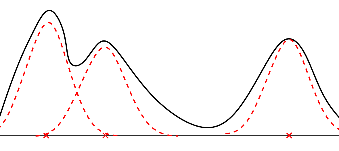
Intuitively speaking, (16) attempts to find the model that can be explained by fewest number of components yet still fits the data well. However, our empirical observation is that the NPMLE selected is often too “noisy” to reveal a clear clustering structure. This is also related to our discussion on the need of a smooth-denoise step in our estimation procedure in Section 3.1. Here we propose a simple remedy via the use of an over-smoothed projection, namely the projection computed with bandwidth :
| (18) |
The motivation comes from the observation in Proposition 2.4 and in Figure 2 that the NPMLEs computed with larger ’s tend to have fewer support atoms. By choosing a larger than that returned by (16), we get a denoising effect. Returning to the examples in Figure 1, the selected model is shown in the last figure in the second row, which has a much clearer structure than in the original data samples.
Selection of Number of Components
Now with the proxy model (18), the remaining step is to cluster its mixing measure to form a partition of the parameter space, based on which we cluster the original data points. In order to proceed, we need to choose the number of clusters and we remark that it is only in this final step that we need .
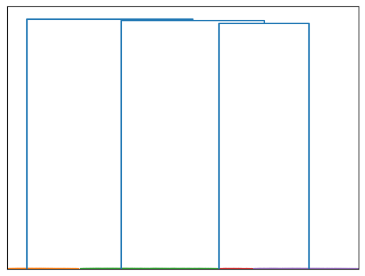
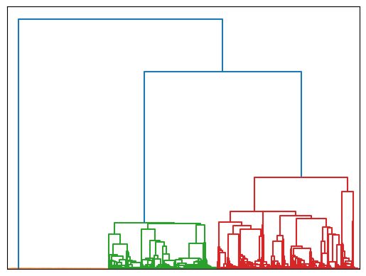
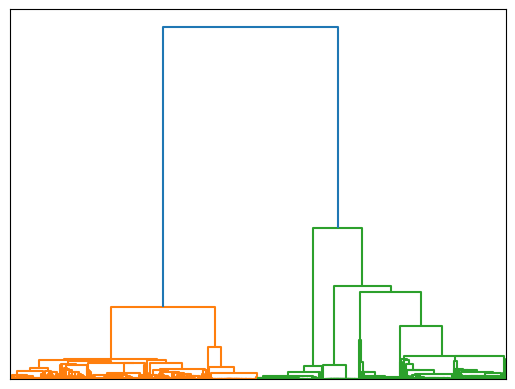
A distinctive feature of our approach is that although we never assume that is a mixture of (potentially nonparametric) components, if has such a structure (approximately), it will be revealed by the steps described above. This can be clearly seen in our motivating example (Figure 1), where the four modes are captured by the dendrogram in Figure 3. A more striking illustration of this can be seen in Figure 6: A hierarchical clustering dendrogram of the raw samples are shown on the left, with no evident clustering structure. Indeed, standard clustering metrics would assign a majority of the samples to a single cluster indicated in red. After running our procedure to select a model , we can view the atoms of as a “denoised” version of the data that more clearly captures the latent structure. Indeed, the dendrogram over these atoms is shown on the right, and from here we can clearly see that there are four clusters in the data; although we emphasize that contains many more than four atoms.
Thus, to find a good candidate for the number of clusters , we shall again exploit the selected model and examine the dendrogram of its support atoms. For the example in Figure 1, the dendrogram of the selected model (Figure 6) clearly suggests a choice of . On the other hand, such information can not be obtained from the dendrogram of the original data samples as shown in Figure 6.
Now suppose that has been selected. We can simply apply single-linkage clustering on the atoms of until clusters are retained. Denoting the resulting clusters of support atoms as , we obtain weighted component densities
| (19) |
The final clustering rule is then defined as the Bayes optimal partition
A complete description of our clustering algorithm can be found in Algorithm 1.
Remark 4.2.
It is clear that Algorithm 1 works for any choice of , whether obtained through the dendrogram, prior knowledge, or some other means.
Numerical Experiments
We investigate numerically the idea of multiscale representation and demonstrate the wide applicability of our clustering algorithm. Before presenting the results, let’s discuss one missing piece from our estimation procedure introduced above, namely how to compute the NPMLE. The original definition (5) gives an infinite dimensional optimization problem and is not directly solvable. Earlier works such as Feng and Dicker (2018) propose to first construct a grid over the parameter space and restrict search to probability measures supported on this grid. This has the advantage of reducing (5) to a convex problem since only the weights of the probability measure needs to be computed, but suffers from the curse of dimensionality as the grid size would scale exponentially with respect to the dimension. Since then, many recent works have been carried out on advancing computational tools for NPMLEs (Zhang et al., 2024, Yan et al., 2024, Yao et al., 2024). In this paper, we shall employ the Wasserstein-Fisher-Rao gradient flow algorithm proposed by (Yan et al., 2024, Algorithm 1). However, we remark this step of computing the NPMLE should be treated as a black-box and any one of the above mentioned algorithms is applicable.
Simulation Studies
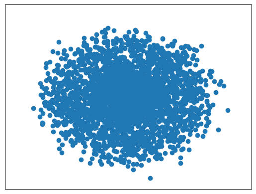
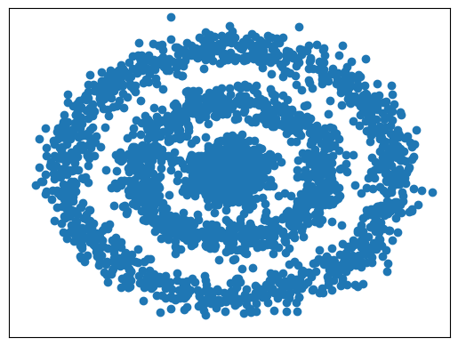
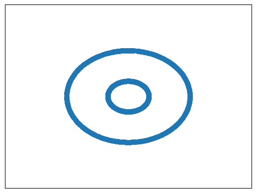
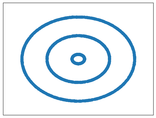
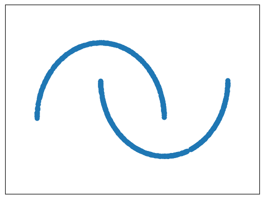
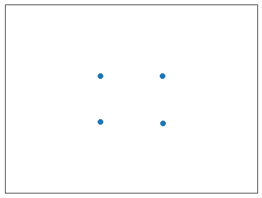
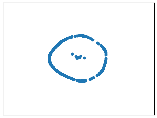
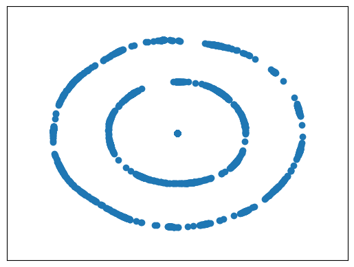
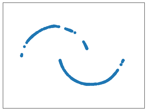
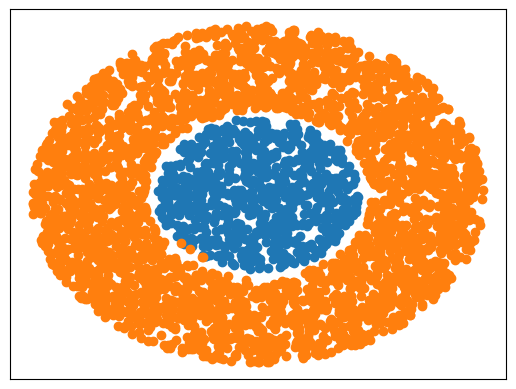
To start with, we shall consider four simulated examples where the density indeed comes from the family of convolutional Gaussian mixtures . These simulations are appealing since there is an easily computed (i.e. known) ground truth to compare with. Moreover, as is clear from Figure 7, this allows us to simulate datasets without a clear clustering structure, despite knowing there is underlying structure. In subsequent sections, we consider benchmarks with no underlying convolutional structure.
We consider the following four examples:
-
1.
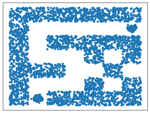
Four squares: , where is a square.
-
2.
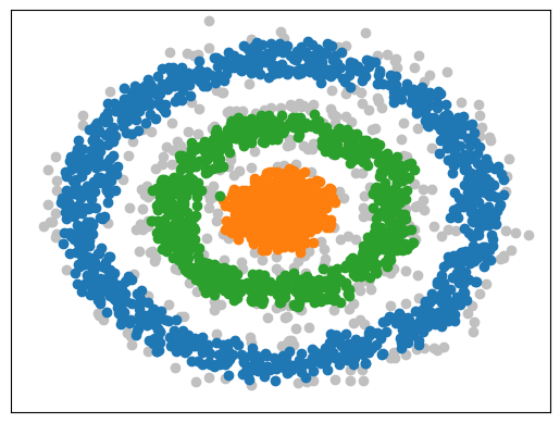
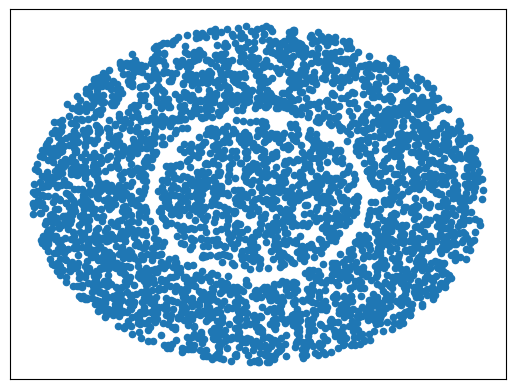
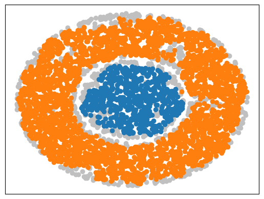
Two concentric circles: , where , is the unit circle.
-
3.
Three concentric circles: , where , is the unit circle.
-
4.
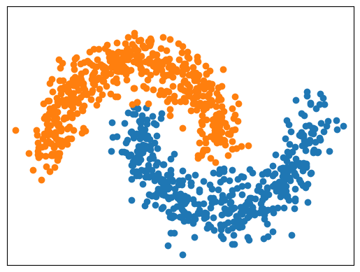
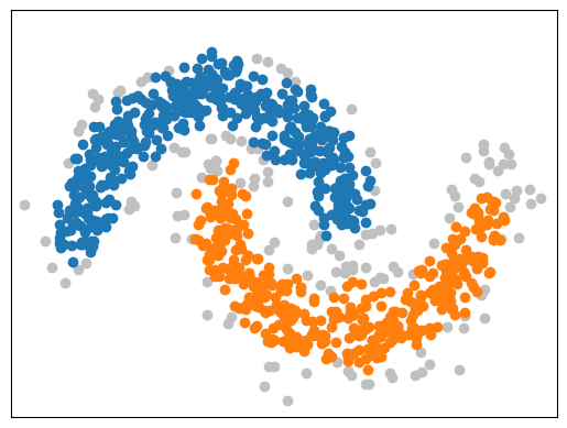
Two moons: , where , is a semi-circle arc.
Figure 7 shows the support of these mixing measures as well as data samples from them.

We shall apply Algorithm 1 to these four dataset and compare its performance with standard clustering algorithms. Firstly, we shall examine the clusters returned by Algorithm 1 without specifying the true number of clusters and compare them with those found by the HDBSCAN algorithm (Campello et al., 2013) since the latter does not require knowledge of either. We recall that our estimate for is based on the dendrograms of the selected NPMLEs, which are both shown in Figure 8.

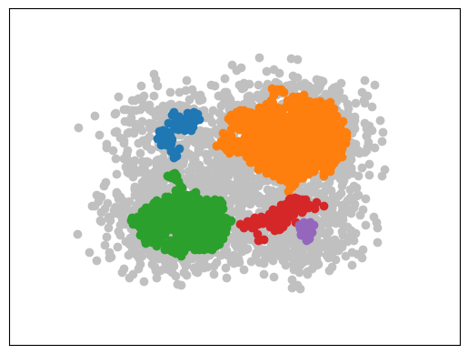
We can see that each one of them has a clear clustering structure as suggested by the dendrograms, based on which we set the number of clusters to be 4,2,4,2 respectively. Figure 9 (top row) shows the resulting clustering of the samples computed as in Algorithm 1, compared with those returned by the HDBSCAN algorithm (bottom row). The gray points in the figures of the bottom row are “noise points” labeled by the HDBSCAN algorithm based on a hyperparameter minPts, which we have tuned to give the best visual results. We can see that our method (Algorithm 1) successfully captures the latent clustering structures in all cases, whereas HDBSCAN does a poorer job for the first two datasets, where the cluster structures are less clear from the raw samples.
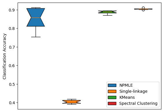
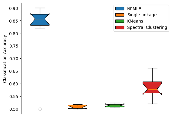
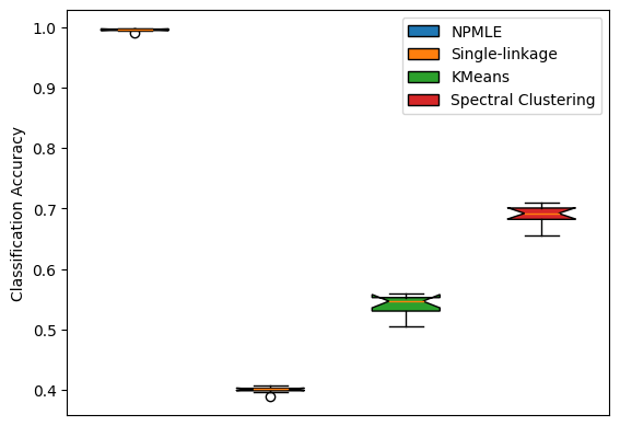
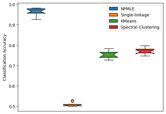
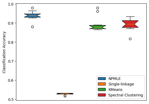
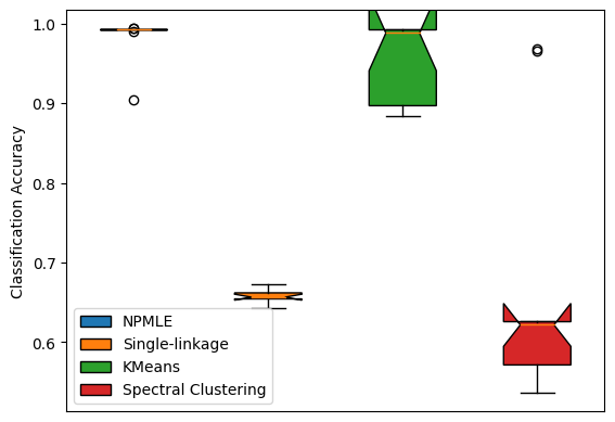
Next, to get a quantitative sense of the performance of Algorithm 1, we shall compare the classification accuracy with standard algorithms such as K-means, single-linkage clustering, spectral clustering. We repeat the experiments 10 times and results are shown in Figure 10. For consistency in comparison, since the other methods also require the number of clusters as input, we provide the true number of clusters for each of the algorithms compared here. We see that our proposed method gives a uniformly good performance across all examples, whereas the other methods give a poor clustering on more than one of them. This suggests that our proposed approach is able to handle a wider range of geometric structures in . Figure 8 also plots the support of the NPMLE returned by our model selection rule. For HDBSCAN, since it does not cluster the noise points and usually gives more clusters than that are present, we choose to not include the comparison in Figure 10. But as can be expected from Figure 9, it also leads to a poor classification accuracy for the first two examples.
Benchmark datasets
After testing our algorithm on simulated datasets with known ground truth, we proceed to consider several benchmark datasets.
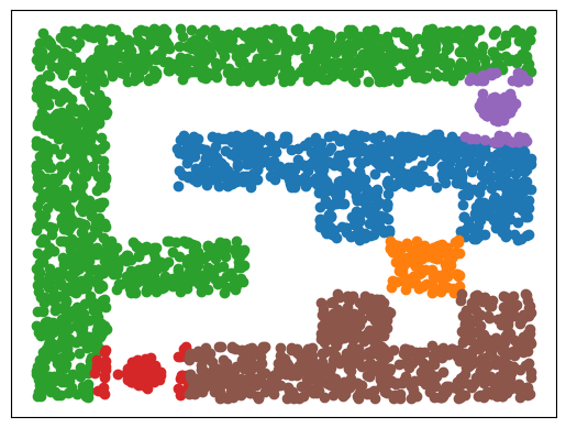
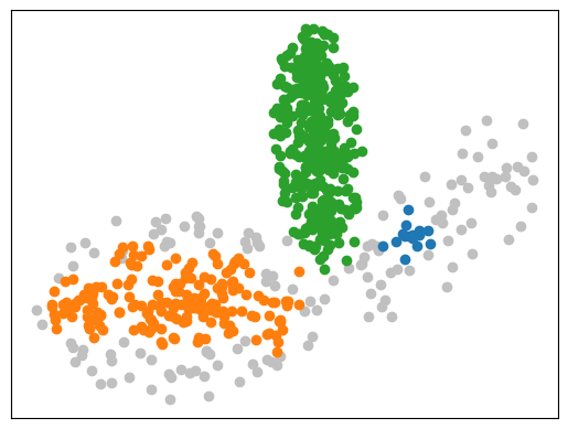
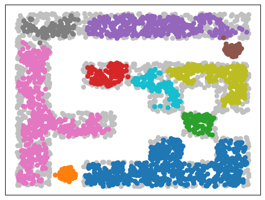
Again, we shall apply Algorithm 1 and compare its performance with the other standard clustering algorithms. Figure 12 shows the selected NPMLEs and the associated dendrograms. We see that there is again clear clustering structures in each of them, and by inspecting the dendrograms, we shall set the number of clusters to be 4,4,2,6 respectively, where the last one comes from the three colored branches and the three single-leaf ones.
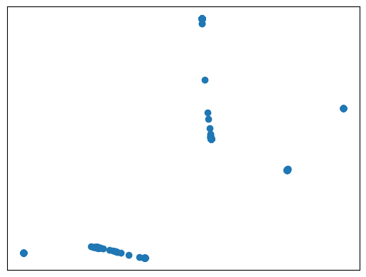
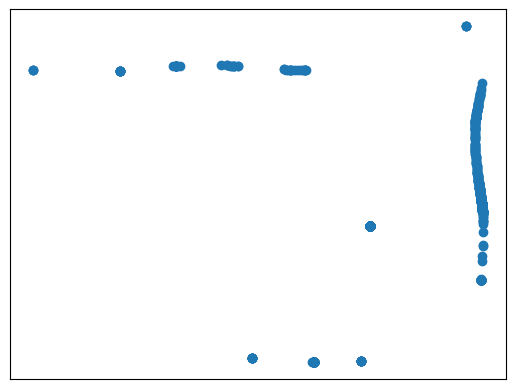
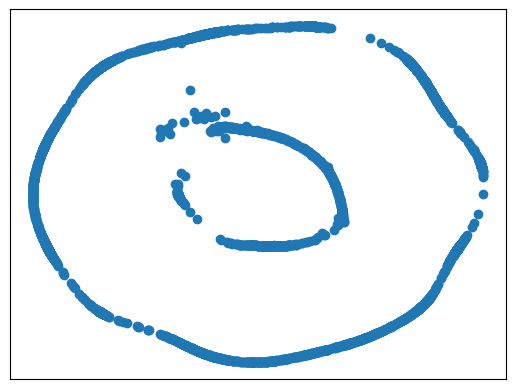
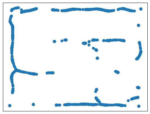
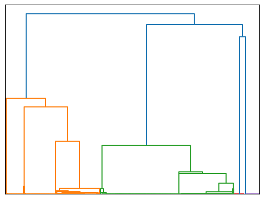
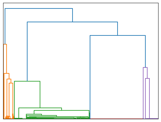
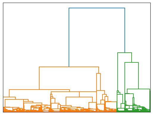
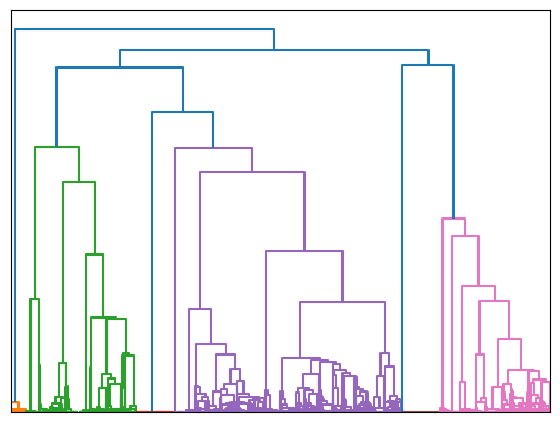
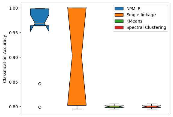
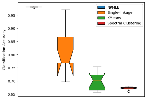
Figure 13 then compares the resulting clustering of the datasets with those found by HDBSCAN. A notable observation is that our approach again captures mostly the major clusters of within the datasets, and outperforms HDBSCAN on the Labyrinth example. The only exception is in the three leaves example, where our algorithm splits rightmost cluster into two. We believe this is due to the imbalanced weights of the three clusters, where only two isolated atoms remain in our selected NPMLE for representing the rightmost cluster. A similar issue is present in HDBSCAN, where the rightmost portion of the data points are labeled as noise and not clustered correctly. Finally, we give a quantitative measure of the clustering accuracy by comparing with K-means, single-linkage clustering and spectral clustering in Figure 14. Here we repeat the experiment 10 times by subsampling 90% of the original datasets and use the true number of clusters in Algorithm 1. As shown in Figure 14, our proposed method achieves uniformly good performance and outperforms the other algorithms for the latter two examples.
Discussion
We have proposed a recipe for identifying and estimating the latent structures of a general density whenever such structures are present. Our approach is model-free and does not rely on any structural assumptions on the original density. The central idea lies in extracting the latent structures at different scales, encoded as a collection of probability measures computed via nonparametric maximum likelihood estimation. We rigorously characterized the asymptotic limit of such estimators from the perspective of mixture models, and showed that they are strongly consistent. By further incorporating the structural information across different scales, we proposed a model selection procedure that returns a most representative model that turns out to be useful for clustering purposes. The resulting clustering algorithm is able to decipher a wide range of hidden structures in practice. The investigation brings up interesting theoretical questions regarding the geometry of the NPMLE in high-dimensions that present intriguing directions for future work.
References
- Allman et al. [2009] E. S. Allman, C. Matias, and J. A. Rhodes. Identifiability of parameters in latent structure models with many observed variables. The Annals of Statistics, pages 3099–3132, 2009.
- Aragam and Yang [2023] B. Aragam and R. Yang. Uniform consistency in nonparametric mixture models. The Annals of Statistics, 51(1):362–390, 2023.
- Aragam et al. [2020] B. Aragam, C. Dan, E. P. Xing, and P. Ravikumar. Identifiability of nonparametric mixture models and bayes optimal clustering. The Annals of Statistics, 48(4):2277–2302, 2020.
- Banerjee and Ghosal [2015] S. Banerjee and S. Ghosal. Bayesian structure learning in graphical models. Journal of Multivariate Analysis, 136:147–162, 2015.
- Bartlett et al. [2006] P. L. Bartlett, M. I. Jordan, and J. D. McAuliffe. Convexity, classification, and risk bounds. Journal of the American Statistical Association, 101(473):138–156, 2006.
- Belkin et al. [2006] M. Belkin, P. Niyogi, and V. Sindhwani. Manifold regularization: A geometric framework for learning from labeled and unlabeled examples. Journal of machine learning research, 7(11), 2006.
- Bordes et al. [2006] L. Bordes, S. Mottelet, and P. Vandekerkhove. Semiparametric estimation of a two-component mixture model. The Annals of Statistics, 34(3):1204–1232, 2006.
- Campello et al. [2013] R. J. Campello, D. Moulavi, and J. Sander. Density-based clustering based on hierarchical density estimates. In Pacific-Asia conference on knowledge discovery and data mining, pages 160–172. Springer, 2013.
- Chaudhuri and Dasgupta [2010] K. Chaudhuri and S. Dasgupta. Rates of convergence for the cluster tree. Advances in neural information processing systems, 23, 2010.
- Chaudhuri et al. [2014] K. Chaudhuri, S. Dasgupta, S. Kpotufe, and U. Von Luxburg. Consistent procedures for cluster tree estimation and pruning. IEEE Transactions on Information Theory, 60(12):7900–7912, 2014.
- Coretto and Hennig [2023] P. Coretto and C. Hennig. Nonparametric consistency for maximum likelihood estimation and clustering based on mixtures of elliptically-symmetric distributions. arXiv preprint arXiv:2311.06108, 2023.
- Do et al. [2024] D. Do, L. Do, S. A. McKinley, J. Terhorst, and X. Nguyen. Dendrogram of mixing measures: Learning latent hierarchy and model selection for finite mixture models. arXiv preprint arXiv:2403.01684, 2024.
- Dombowsky and Dunson [2023] A. Dombowsky and D. B. Dunson. Bayesian clustering via fusing of localized densities. arXiv preprint arXiv:2304.00074, 2023.
- Drton and Maathuis [2017] M. Drton and M. H. Maathuis. Structure learning in graphical modeling. Annual Review of Statistics and Its Application, 4(1):365–393, 2017.
- Elmore et al. [2005] R. Elmore, P. Hall, and A. Neeman. An application of classical invariant theory to identifiability in nonparametric mixtures. In Annales de l’institut Fourier, volume 55, pages 1–28, 2005.
- Ester et al. [1996] M. Ester, H.-P. Kriegel, J. Sander, X. Xu, et al. A density-based algorithm for discovering clusters in large spatial databases with noise. In kdd, volume 96, pages 226–231, 1996.
- Feng and Dicker [2018] L. Feng and L. H. Dicker. Approximate nonparametric maximum likelihood for mixture models: A convex optimization approach to fitting arbitrary multivariate mixing distributions. Computational Statistics & Data Analysis, 122:80–91, 2018.
- Fraley and Raftery [2002] C. Fraley and A. E. Raftery. Model-based clustering, discriminant analysis, and density estimation. Journal of the American statistical Association, 97(458):611–631, 2002.
- Gassiat and Rousseau [2016] E. Gassiat and J. Rousseau. Nonparametric finite translation hidden markov models and extensions. Bernoulli, pages 193–212, 2016.
- Genovese and Wasserman [2000] C. R. Genovese and L. Wasserman. Rates of convergence for the gaussian mixture sieve. The Annals of Statistics, 28(4):1105–1127, 2000.
- Ghosal and Van Der Vaart [2001] S. Ghosal and A. W. Van Der Vaart. Entropies and rates of convergence for maximum likelihood and bayes estimation for mixtures of normal densities. The Annals of Statistics, 29(5):1233–1263, 2001.
- Guha et al. [2021] A. Guha, N. Ho, and X. Nguyen. On posterior contraction of parameters and interpretability in bayesian mixture modeling. Bernoulli, 27(4):2159–2188, 2021.
- Hall and Zhou [2003] P. Hall and X.-H. Zhou. Nonparametric estimation of component distributions in a multivariate mixture. The Annals of Statistics, 31(1):201–224, 2003.
- Hall et al. [2005] P. Hall, A. Neeman, R. Pakyari, and R. Elmore. Nonparametric inference in multivariate mixtures. Biometrika, 92(3):667–678, 2005.
- Hartigan [1981] J. A. Hartigan. Consistency of single linkage for high-density clusters. Journal of the American Statistical Association, 76(374):388–394, 1981.
- Hastie et al. [2015] T. Hastie, R. Tibshirani, and M. Wainwright. Statistical learning with sparsity. Monographs on statistics and applied probability, 143(143):8, 2015.
- Hunter et al. [2007] D. R. Hunter, S. Wang, and T. P. Hettmansperger. Inference for mixtures of symmetric distributions. The Annals of Statistics, pages 224–251, 2007.
- Jang and Jiang [2019] J. Jang and H. Jiang. Dbscan++: Towards fast and scalable density clustering. In International conference on machine learning, pages 3019–3029. PMLR, 2019.
- Juditsky et al. [2009] A. B. Juditsky, O. Lepski, and A. B. Tsybakov. Nonparametric estimation of composite functions. Annals of Statistics, 37(3):1360–1404, 2009.
- Kiefer and Wolfowitz [1956] J. Kiefer and J. Wolfowitz. Consistency of the maximum likelihood estimator in the presence of infinitely many incidental parameters. The Annals of Mathematical Statistics, pages 887–906, 1956.
- Lee and Hastie [2015] J. D. Lee and T. J. Hastie. Learning the structure of mixed graphical models. Journal of Computational and Graphical Statistics, 24(1):230–253, 2015.
- Lin and Zha [2008] T. Lin and H. Zha. Riemannian manifold learning. IEEE transactions on pattern analysis and machine intelligence, 30(5):796–809, 2008.
- Lindsay [1983a] B. G. Lindsay. The geometry of mixture likelihoods, part ii: the exponential family. The Annals of Statistics, 11(3):783–792, 1983a.
- Lindsay [1983b] B. G. Lindsay. The geometry of mixture likelihoods, part ii: the exponential family. The Annals of Statistics, 11(3):783–792, 1983b.
- Lindsay [1995] B. G. Lindsay. Mixture models: Theory, geometry and applications. In NSF-CBMS Regional Conference Series in Probability and Statistics, pages i–163. JSTOR, 1995.
- McLachlan and Chang [2004] G. McLachlan and S. Chang. Mixture modelling for cluster analysis. Statistical methods in medical research, 13(5):347–361, 2004.
- McNicholas [2016] P. D. McNicholas. Model-based clustering. Journal of Classification, 33:331–373, 2016.
- Melnykov and Maitra [2010] V. Melnykov and R. Maitra. Finite mixture models and model-based clustering. Statistics Surveys, 4:80–116, 2010.
- Nguyen [2013] X. Nguyen. Convergence of latent mixing measures in finite and infinite mixture models. The Annals of Statistics, 41(1):370–400, 2013.
- Polyanskiy and Wu [2020] Y. Polyanskiy and Y. Wu. Self-regularizing property of nonparametric maximum likelihood estimator in mixture models. arXiv preprint arXiv:2008.08244, 2020.
- Ramsay [1998] J. O. Ramsay. Estimating smooth monotone functions. Journal of the Royal Statistical Society: Series B (Statistical Methodology), 60(2):365–375, 1998.
- Roeder [1990] K. Roeder. Density estimation with confidence sets exemplified by superclusters and voids in the galaxies. Journal of the American Statistical Association, 85(411):617–624, 1990.
- Saha and Guntuboyina [2020] S. Saha and A. Guntuboyina. On the nonparametric maximum likelihood estimator for gaussian location mixture densities with application to gaussian denoising. The Annals of Statistics, 48(2):738–762, 2020.
- Schwarz [1978] G. Schwarz. Estimating the dimension of a model. Annals of Statistics, 6(2):461–464, 1978.
- Soloff et al. [2024] J. A. Soloff, A. Guntuboyina, and B. Sen. Multivariate, heteroscedastic empirical bayes via nonparametric maximum likelihood. Journal of the Royal Statistical Society Series B: Statistical Methodology, page qkae040, 2024.
- Sriperumbudur and Steinwart [2012] B. Sriperumbudur and I. Steinwart. Consistency and rates for clustering with dbscan. In Artificial Intelligence and Statistics, pages 1090–1098. PMLR, 2012.
- Stahl and Sallis [2012] D. Stahl and H. Sallis. Model-based cluster analysis. Wiley Interdisciplinary Reviews: Computational Statistics, 4(4):341–358, 2012.
- Steinwart [2011] I. Steinwart. Adaptive density level set clustering. In Proceedings of the 24th Annual Conference on Learning Theory, pages 703–738. JMLR Workshop and Conference Proceedings, 2011.
- Steinwart [2015] I. Steinwart. Fully adaptive density-based clustering. The Annals of Statistics, 43(5):2132–2167, 2015.
- Stuetzle and Nugent [2010] W. Stuetzle and R. Nugent. A generalized single linkage method for estimating the cluster tree of a density. Journal of Computational and Graphical Statistics, 19(2):397–418, 2010.
- Tai and Aragam [2023] W. M. Tai and B. Aragam. Tight bounds on the hardness of learning simple nonparametric mixtures. In The Thirty Sixth Annual Conference on Learning Theory, pages 2849–2849. PMLR, 2023.
- Villani [2009] C. Villani. Optimal Transport: Old and New, volume 338. Springer, 2009.
- Wolfe [1970] J. H. Wolfe. Pattern clustering by multivariate mixture analysis. Multivariate behavioral research, 5(3):329–350, 1970.
- Yan et al. [2024] Y. Yan, K. Wang, and P. Rigollet. Learning gaussian mixtures using the wasserstein–fisher–rao gradient flow. The Annals of Statistics, 52(4):1774–1795, 2024.
- Yao et al. [2024] R. Yao, L. Huang, and Y. Yang. Minimizing convex functionals over space of probability measures via kl divergence gradient flow. In International Conference on Artificial Intelligence and Statistics, pages 2530–2538. PMLR, 2024.
- Zhang [2009] C.-H. Zhang. Generalized maximum likelihood estimation of normal mixture densities. Statistica Sinica, pages 1297–1318, 2009.
- Zhang et al. [2024] Y. Zhang, Y. Cui, B. Sen, and K.-C. Toh. On efficient and scalable computation of the nonparametric maximum likelihood estimator in mixture models. Journal of Machine Learning Research, 25(8):1–46, 2024.
Appendix A Proof of Proposition 2.1
First of all, let’s point out that the minimization in (6) is equivalent to the following maximization problem:
| (20) |
Notice that densities in are uniformly bounded above, so that the maximum (20) exists. To establish existence of the maximizer, we claim that is compact when equipped with the metric. We need the following result.
Proposition A.1.
Let be compact. The space is compact for
Proof.
Since is compact, it is known that is weakly compact. By [Villani, 2009, Corollary 6.13], the weak convergence is equivalent to convergence in since the Euclidean distance on is a bounded metric. Therefore the result follows. ∎
To show is compact, let be a sequence. By compactness of established in Proposition A.1, the sequence converges in along a subsequence to a point . By Lemma F.2 below, since , this implies that converges in along the same subsequence towards , establishing compactness.
Now let be a sequence in such that . By compactness of , there is a subsequence such that in norm, so that along a further subsequence (still denoted as ) pointwise almost everywhere. Now consider the sequence of non-positive functions , which converges pointwise almost everywhere to . By Fatou’s lemma for non-positive functions, we obtain
Therefore attains the maximum.
Finally, uniqueness follows from the strict concavity of . Indeed, let and be two distinct maximizers of . Then by convexity of , and we have
a contradiction.
Appendix B Proof of Proposition 2.2
Proof of Proposition 2.2.
Let be fixed. We shall show that belongs to the ball for all large, thereby establishing the result.
Fix . For any , we claim that there exists such that
Indeed, we have
Here the step (S1) follows from the monotonicity of the sequence. Step (S2) uses Fatou’s lemma, which is indeed applicable here since the integrand is lower bounded by . Step (S3) follows from the fact that for all if , which is because convergence in metric implies weak convergence and the function as a function of is bounded continuous. Step (S4) uses the concavity of . The step (S5) follows from the observation that
which is equivalent to
Now with the claim, we can form an open cover of the set by using the open balls with ranging over . Since is closed and hence compact by Proposition A.1, we obtain a finite open cover so that
The by law of large numbers, we have that almost surely
for all large enough ’s. In other words, for all , we have
Since , the above inequality implies that any cannot attain the maximum likelihood over . Therefore must be an element of . ∎
Appendix C Proof of Proposition 2.4
Let’s first review a characterization of the number of support atoms for the NPMLE, where we recall that
where are i.i.d. samples from the true density . It can be shown that [see .e.g Lindsay, 1995, Chapter 5] the maximizer is a discrete measure with at most atoms and
where
Therefore it suffices to characterize the critical points of , which reads in our case as
| (21) |
where . The following lemma mimics the proof of [Polyanskiy and Wu, 2020, Theorem 3] by keeping track of and then proves Proposition 2.4.
Lemma C.1.
Let and . Define . We have
Proof.
We need to study the zeros of the gradient of (21), which takes the form
Therefore it suffices to study the zeros of the function
where the , normalized so that . A first observation is that the zeros of all lie in the interval because is strictly positive (and negative) over (resp. ). Let and consider
Notice that the real roots of over coincide with the real roots of over , where . Now we shall apply the following result from [Polyanskiy and Wu, 2020, Lemma 4] to bound the number of zeros of over the disc .
Lemma C.2.
Let be a non-zero holomorphic function on a disc of radius . Let and . For any , we have
Let , , where is to be determined. Notice that
where is a discrete random variable defined as and . Since and , we have
Similarly, we have
Therefore we have
Setting and with , we get
Setting , , we get
∎
The second assertion follows from [Lindsay, 1983a, Theorem 4.1] by noting that if , then the mixture quadratic, which takes the form of , is strictly positive for all . Hence the NPMLE with be the delta measure at the mean.
Appendix D Proof of Lemma 3.3
Let and be the -enlargement of . We remark that convergence in does not guarantee that the atoms in are as separated as in (11). We shall need the following result gives a bound on the total weight of the outlier atoms of .
Lemma D.1 (Lemma 5.3 of Aragam and Yang [2023]).
Let and . Then
First of all, let’s point out that is a non-vanishing density over . Indeed, for any , there exists a set of positive measure so that over for some . Then it follows that
Next, we shall establish an upper bound on when is away from the support of . By the definition of , we have
where as in Lemma D.1. Now for any such that , we have for any and so the second sum in the above equals zero. In particular we have shown that
| (22) |
Therefore, this suggests a threshold and we can then write
| (23) | ||||
Next, we shall show that each is almost a connected set. To accomplish this, we need a bound on . Let be any coupling between and
To bound the term , it suffices to upper bound the non-overlapping volumes between the supports of the two box kernels, which is bounded by twice the sum of hyperrectangles each with side length and . Therefore we have
and hence
It follows that the measure of the set is bounded by
| (24) |
Now notice that we have
and hence
where the last step is the definition of in (23). We shall show that the left hand side is almost an connected set when is large. Indeed, since is non-vanishing over , the set will eventually become . Similarly, the fact (24) that (as a subset of the compact set ) has vanishing measure implies that it shrinks towards the empty set. Therefore, by intersecting with , we only introduce tiny “holes” whose sizes converge to zero. In other words, we have shown that
where is a set whose Lebesgue measure converges to zero.
Appendix E Proof of Lemma 3.4
If we view each as a union of open sets , then the condition (13) together with the separation assumption (11) further suggests that the pairwise distances among is less than the distance between any and for Therefore, if we apply single-linkage clustering to all the disjoint open subsets in until clusters remain, then we shall recover the ’s. Furthermore, our construction of the ’s in Definition 3.2 suggests that if we continue merging the open subsets in ’s until clusters are retained, we should obtain the similar guarantees that
Now to prove the second part, we need to show that for any , for all .
Upper bound on :
Let be a point such that . Then
Since , for some . By (13), we have when is large, which further implies that because is simply a union of the corresponding ’s including . Therefore we have .
Lower bound on for :
Let be a point such that . Let and be such that . Then by (11)
so that
| (25) |
when is large. Combining this with the upper bound on establishes the lemma.
Appendix F Proof of Theorem 3.5
The proof of Theorem 3.5 relies on the following proposition, which combined with Proposition 2.2 gives the result.
Proposition F.1.
We have
where is a constant depending on .
Proof.
To simplify the notation, we will suppress the dependence of on and denote them as . First we notice that to bound and , it suffices to bound . Indeed we have
and
so that
| (26) |
Now we shall focus on , which we decompose as three terms by introducing a mollifier
where
Here is a symmetric density function with bounded first moment whose Fourier transform is supported in and .
Bound for : Recall with . Then and
We have
By [Nguyen, 2013, Lemma 1], we have
| (27) |
where the last step can be proved as in [Nguyen, 2013, Theorem 2]: letting and gives . For we have
where
Recall that so we have . Then for
and hence . For , we have
Therefore
| (28) |
and further that
| (29) |
Combining (27), (28) and (29) we get
| (30) |
where as in Lemma D.1.
Bound for : The term can be bounded similarly as
| (31) |
Note that since the support of is , the corresponding error term is zero.
Bound for : Let .
The second term can be bounded by noticing that
and similarly for . The first term can be bounded using Cauchy-Schwarz by
Letting (since is continuous and compactly supported, and is never zero, and is well-defined), we have and then
Thus by Young’s inequality we have
and by Plancherel’s identity
where we have used the fact that is bounded supported on , which implies that is supported on . Therefore we have
| (32) |
and furthermore by combining (30), (31), (32) we have
Setting , we get
where we have used Lemma F.2 below to bound and the fact that . This finishes the proof with (26).
∎
Lemma F.2.
Let . Then
Proof.
Let be a coupling between and . Then
with
Then we have
where taking the infimum over all couplings gives the desired result. ∎