Optimizing and Managing Wireless Backhaul for Resilient Next-Generation Cellular Networks

Abstract

Next-generation wireless networks target high network availability, ubiquitous coverage, and extremely high data rates for mobile users. This requires exploring new frequency bands, e.g., mmWaves, moving toward ultra-dense deployments in urban locations, and providing ad hoc, resilient connectivity in rural scenarios. The design of the backhaul network plays a key role in advancing how the access part of the wireless system supports next-generation use cases. Wireless backhauling, such as the newly introduced Integrated Access and Backhaul (IAB) concept in 5G, provides a promising solution, also leveraging the mmWave technology and steerable beams to mitigate interference and scalability issues. At the same time, however, managing and optimizing a complex wireless backhaul introduces additional challenges for the operation of cellular systems. This paper presents a strategy for the optimal creation of the backhaul network considering various constraints related to network topology, robustness, and flow management. We evaluate its feasibility and efficiency using synthetic and realistic network scenarios based on 3D modeling of buildings and ray tracing. We implement and prototype our solution as a dynamic IAB control framework based on the Open RAN architecture, and demonstrate its functionality in Colosseum, a large-scale wireless network emulator with hardware in the loop.

I Introduction

Next-generation cellular networks will be deployed in a variety of operational environments (e.g., ultra-dense urban, rural) [1], supported by heterogeneous Radio Access Technologies (RATs) [2], and operating in different portions of the spectrum [3]. As an example, urban cellular networks are moving toward a 10-fold increase in the density of Next Generation Node Bases (gNBs), from 10 gNBs per km² typically deployed today to an estimated 100 gNBs per km² in 5G [4].

The diverse characteristics of these access scenarios introduce new challenges for the design of a robust and high performance backhaul network, which needs to be pervasive and flexible. Traditional backhaul solutions, based on fiber drops or point-to-point dedicated wireless links to each RAN base station, are limited in terms of scalability and cost, and are often referred to as one of the barriers toward both ultra-dense deployments in urban areas and remote, rural access. For these reasons, the 3rd Generation Partnership Project (3GPP) has introduced native support for wireless backhaul in Release 16 for its 5th generation (5G) cellular technology, i.e., 3GPP NR. Specifically, IAB introduces wireless self-backhauling with the same waveform and protocol stack already used for the access part of the network [5, 6]. With IAB, only some of the gNBs need to be fiber-connected (i.e., the IAB-donors), and a wireless multi-hop network topology connects every other gNB (i.e., the IAB-nodes) to the closest donor. IAB networks are thus organized in multiple trees, with roots in different donors and leaves represented by the User Equipments (UEs).

Wireless self-backhaul, integrated with the access network, significantly improves the flexibility of cellular deployments for 5G and beyond, but, at the same time, adds complexity in the management plane and needs to be properly designed and deployed to offer the best performance to the end users of the network. On one hand, IAB in 5G and beyond can leverage the new spectrum above 6 GHz, in the lower millimeter wave (mmWave) band, to increase the capacity of the system [3] and to limit self-interference thanks to highly directional transmissions from large antenna arrays in the IAB nodes. On the other, mmWave links present a 15 dB to 30 dB gap in received power between Line-of-Sight (LOS) and Non-Line-of-Sight (NLOS) conditions [3, 7], thus requiring careful planning that favors LOS links and avoids blockage conditions [8, 9]. Similarly, the opportunity of re-using the same frequency bands for access and backhaul provides a potential multiplexing gain, but also challenges for scheduling of data flows across the two parts of the network [10]. Finally, self-backhaul solutions extend the scenarios in which access connectivity can be provided, but at the same time a failure in a wireless backhaul link has a more significant impact than a failure of a single access link, as it impacts all the downstream nodes in the topology tree.

These reasons make design and optimization of IAB networks critical parts of next-generation wireless planning and operations. In this paper, we focus on pre-deployment and post-deployment approaches for the optimal identification and management of topologies across complex IAB networks, with the goal of (i) providing a minimum guaranteed area capacity, in line with the International Telecommunication Union (ITU) recommendations for next-generation cellular networks [4]; and (ii) minimizing the downtime of the IAB tree in case of failures of links between parent and child IAB nodes. Specifically, our contributions are as follows:

• We introduce mixed Integer-Linear Problems (ILPs) that combine topological, resiliency, and flow constraints, which we test on synthetic graphs and realistic topologies derived by 3D surfaces representing real world urban areas. Using accessible hardware, we achieve near-optimal solutions for fault-tolerant synthetic topologies up to 45 nodes, and up to 60 nodes for realistic topologies. In both cases we measure a lower bound on the required percentage of donors around 20%.

• We prototype the network optimization and management routine on an O-RAN rApp (i.e., a piece of custom control logic running in the O-RAN Non-real-time (Non-RT) RAN Intelligent Controller (RIC) [11, 12]). The rApp dynamically recreates the IAB topology in case of link failures in the backhaul topology, based on the guidance from the optimization problem. We use Colosseum [13], the world’s largest wireless network emulator with hardware-in-the-loop, to confirm the viability of our approach in an experimental network based on the open-source OAI 5G protocol stack [11].

We believe that the proposed approaches and test methodology is an important step toward the practical management and optimization of scalable, resilient, high-performance wireless self-backhaul solutions in realistic deployments.

II State of The Art

Tezergil et al. recently surveyed the theme of planning wireless 5G backhaul networks [14]. In this section, we review the papers with assumptions comparable to those used in our paper.

Saha and Dhillon [8] use stochastic geometry to derive general results; however, their approach is intrinsically limited to 2-hop backhaul paths and relies on Poisson point process-based deployments, which do not include a real-world deployment assessment, unlike our proposed approach which includes real-world data validation. Lai et al. [15] present results based on random node placement, assuming a-priori knowledge of users’ positions. In contrast, our approach does not require such assumptions, making it more broadly applicable. Madapatha et al. [16], Pagin et al. [17], and Yuan et al. [18] focus on optimizing backhaul topology and scheduling once the IAB-donors are already placed. This presents a less generic and easier-to-solve problem compared to the joint optimization of placement and backhaul links that we tackle in our work. Zhang et al. [19] optimize scheduling fairness; Gopalam et al. [20] develop a distributed algorithm for scheduling optimization; Ma et al. [21] jointly optimize the scheduling of access and backhaul links; and Zhang et al. [22] optimize spectrum and power allocation. All these works, however, operate on a fixed network topology, whereas our work jointly optimizes both topology and backhaul scheduling, adding flexibility to the solution. Islam et al. [23, 24] propose an ILP model for optimizing the placement of IAB-donors and link allocations to maximize flow, without minimizing cost while guaranteeing flow. In contrast, our approach also incorporates robustness, a critical factor for practical deployment, which is absent from their model. Mcmenamy et al. [25] employ a similar approach by limiting the number of hops towards terminals before allocating links among IAB nodes. However, their method is suboptimal, whereas we demonstrate that our approach achieves optimality in more than 90% of real networks and near-optimal results in the remaining cases.

Like our work, these papers assume that backhaul links that do not share an edge are non-interfering due to the use of mmWave links and highly directive beamforming.

In summary, our work is original because it: (i) jointly addresses the problem of IAB-donor placement and backhaul optimization; (ii) tackles both topology and flow optimization together; (iii) introduces robustness into the backhaul; (iv) provides an optimal, not heuristic, solution; (v) uses real data and testbeds rather than random node placements in empty scenarios; and (vi) delivers a working prototype on a realistic testbed integrated into the O-RAN architecture.

III IAB Optimization — Problem Statement

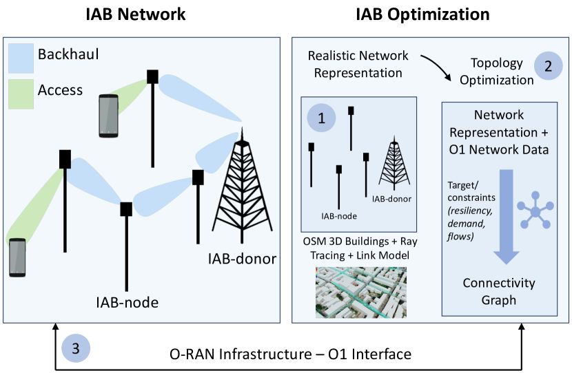
Figure 1: System model of the IAB closed-loop management optimization using the (i) realistic topologies representations; (ii) graph-based optimization; and (iii) the O-RAN infrastructure.

This section introduces the proposed system model for the design of optimal, resilient, and reconfigurable IAB topologies. Our solution pushes forward the state of the art and is practically implementable on available hardware and present standards. Figure 1 depicts the building blocks we rely on. First, we leverage realistic representations of the areas where the IAB network operates. Second, we develop optimization techniques that deploy optimal connectivity graphs over such topologies, including redundant paths to enforce network resiliency. Third, we leverage the O-RAN architecture, and, specifically, the O1 interface between the RAN and the Non-RT RIC, to perform reconfigurations of the network in case of failures.

III-A Realistic Deployment Area Representation

We start from a 3D surface representing with high fidelity the deployment area. This approach has been recently adopted in various papers, e.g., to study localization [26], network planning [27], and LoS estimation [28]. We use open data from public administrations and the OpenStreetMap (OSM) buildings project [29]. In this paper we use the methodology and heuristic proposed in [27] to deploy a network of gNBs in an outdoor urban area, and we then evaluate LoS and link capacity between the gNB similarly to [28]. Given a certain urban scenario and a desired density of gNB per square kilometer, we identify the positions of the gNBs that provide optimal outdoor coverage and the availability of links between gNBs.

We also leverage a realistic traffic demand profile, based on the knowledge of the area covered by each gNB and requirements for next-generation wireless systems, as we detail in Section IV-A, and a link model based on parameters for 3GPP systems and the OAI reference implementation, as discussed in Section IV-B. In the remainder of the paper, we focus on a IAB network deployed at mmWaves, to evaluate the impact of large bandwidth availability to the performance of the system.

III-B Topology Optimization

The optimization uses the given positions of gNBs and creates an optimal IAB backhaul with the minimum number of IAB-donors, which require fiber connectivity to the core network. We follow the IAB specifications that support a backhaul network made of multiple loop-free trees rooted in IAB-donors. The optimization is performed before deploying the network, as it determines the nodes with wired access and those using a wireless backhaul. However, it produces redundant topologies that can be reconfigured at run-time to repair failures.

We consider a directed network graph $G(\mathcal{N}_{v},\mathcal{E}_{v})$, such as the one shown in Fig. 2, that represents the backhaul network, made of a set $\mathcal{N}_{v}$ of gNBs and a set $\mathcal{E}_{v}$ of potential edges, i.e., edges that can be used for the backhaul. The first goal of the optimization is to find the smallest number of IAB-donors, i.e., the smallest subset $\mathcal{N}^{*}\subseteq\mathcal{N}_{v}$ that must be connected to the core network with a wired connection. The second goal is to choose the subset $\mathcal{E}^{*}\subseteq\mathcal{E}_{v}$ of edges that create a multi-hop path from every gNBs in $\mathcal{N}_{v}$ to some IAB-donor. The resulting topology must respect some performance and reliability requirements. Altogether, the final goal is to define $\mathcal{N}^{*}$ and a new graph $G^{*}(\mathcal{N}_{v},\mathcal{E}^{*})$ made of all the gNBs and the set $\mathcal{E}^{*}$ of edges resulting from the union of all the edges of all the trees. We will impose two classes of constraints: topological constraints that impose reliability features and flow conservation based on the estimated link capacity and traffic demand of every gNB. Reliability is one of the key features of 5G, and our approach can be parameterized in order to provide the desired level of redundancy.

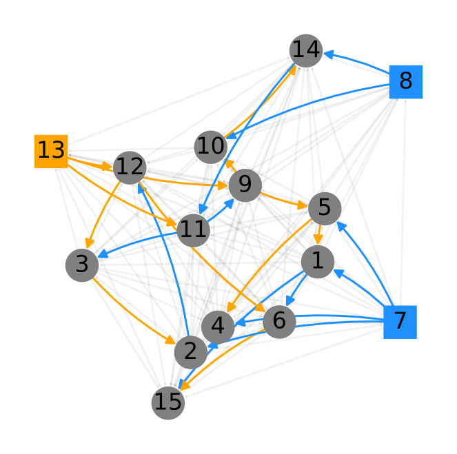
Figure 2: An example realization of the backhaul graph with $R=2$. Circles are IAB-nodes, squares are IAB-donors, orange/blue edges are backhaul links in two disjoint edge-set, gray edges are all the potential edges. Every gray node has two incoming edges.

III-C Open RAN for Optimized IAB Deployments

This generated graph is used to optimally deploy the IAB network in the first instance, but also to manage the network through primitives and capabilities provided by the O-RAN architecture depicted in Fig. 1. O-RAN introduced the Non-RT RIC, which performs optimization and service provisioning with a closed-loop control with a granularity higher than 1s, and connects to the RAN through the O1 interface. The control logic is defined by custom applications called rApps [30]. The O-RAN architecture has been recently extended to support IAB operations, with the interfaces to the RICs (e.g., O1) implemented as tunnels over the backhaul network [11].

The IAB rApp is used in two phases. For network setup, it configures each network component based on the optimized topology. Then, it continuously receives performance metrics and failure events through the O1 interface, and uses them to detect relevant changes in the network topology (e.g., the degradation of a radio link). The rApp reacts by reconfiguring the IAB topology based on the optimization output. We prototype the rApp on Colosseum, a wireless network emulator that includes 256 Software-defined Radio (SDR) together with a digital channel emulator to run large-scale experiments [13], and showcase how network reconfigurability can be achieved.

IV Estimating Demand and Link Capacity

The starting point of our analysis is a 3D model of existing urban areas (obtained using open data) over which we apply state of the art algorithms to decide a placement of gNBs that can guarantee the best ground coverage using LoS links [27]. We then need to estimate the traffic demand for every gNB, and the link capacity that every point-to-point link between gNBs can offer. This will create the annotated graph $G(\mathcal{N}_{v},\mathcal{E}_{v})$ over which we run the optimization. Both estimations are data-driven and are part of our original methodology.

IV-A Estimating Demand

The ITU provides precise parameters to simulate gNB deployments when offering “extended mobile broadband” services [4], which correspond to 10 UE per gNB, each one with a demand of at least 100 Mb/s, so each gNB should be able to serve a load $\lambda=1000$ Mb/s. This work focuses on the coverage of outdoor public areas, so assigning a fixed load per gNB is realistic only if the goal is to minimize coverage overlap in a context where gNBs can be deployed without constraints. However, in scenarios based on actual topographies, as those used in this paper, the buildings make the area of interest nonhomogeneous, with some gNBs that are placed in positions that cover specific areas that would otherwise be significantly shadowed [31]. As a result, coverage areas are often partially overlapping and the UEs may be shared among gNBs. This calls for a strategy to model shared demand among gNBs.

We sample the area under analysis with one point per square meter. From the initial placement algorithm, we obtain $\Sigma=\{\sigma^{0}\ldots\sigma^{n}\}$ that is a family of sets. $\sigma^{i}$ includes all the discrete $(x,y)$ coordinates on the ground that are covered by gNB $i\in\mathcal{N}_{v}$. We restrict $\sigma^{i}$ to the points on the ground that are in LoS with the gNB $i$, as we focus on a mmWave deployment, but the same approach can be used with a different definition (i.e., all the points with a minimum estimated capacity). The area occupied by $\sigma^{i}$ is then simply $|\sigma^{i}|$ (the number of points in the sampled 2D space). One point can belong to more than one set, so we define the multiplicity $m_{x,y}=|\{\sigma^{i}\in\Sigma\;|\;(x,y)\in\sigma^{i}\}|$. We define the demand $d_{i}$ of a gNB as:

$$d_{i}=\frac{|\sigma^{i}|\lambda}{\sum_{(x,y)\in\sigma^{i}}m_{x,y}}$$ (1)

Note that if $\sigma^{i}$ is not overlapping with any other $\sigma^{j}$, then $m_{x,y}=1\;\forall\;(x,y)\in\sigma^{i}$ and $d_{i}=\lambda$, while if gNB $i$ covers an area that overlaps with some other gNB (as it happens for the majority of the real-world scenarios) then $d_{i}<\lambda$.

IV-B Link Capacity Estimation

To estimate the capacity of each link between a pair of nodes $(s,d)$, we model the propagation through a ray tracing analysis using the MATLAB suite, and combine a link abstraction model based on the physical layer implementation of OAI. First, we load the 3D model of the buildings obtained from OSM Buildings, then for each pair of gNBs we perform ray tracing using the shooting and bouncing method [32]. We consider up to a maximum of 4 reflections and we ignore the effect of diffraction that is negligible at mmWave frequencies [33].

For each pair $(s,d)$ we obtain a set $\Gamma$ of rays, each ray $r$ is associated with a pathloss ($P_{r}$), a phase $\Phi_{r}$, a delay ($\delta_{r}$), the angle of arrival and the angle of departure of the ray ($AoA_{r}$, and $AoD_{r}$). Each gNB uses with a uniform planar array antenna, with $8\times 8$ isotropic antenna elements spaced at half wavelength distance. The channel matrix $\mathbf{H}$ is [33]

$$\mathbf{H}=\sum_{r=1}^{\Gamma}\sqrt{P_{r}}~{}e^{j(-2\pi\delta_{r}f_{c}+\Phi_{r}})~{}\mathbf{a}_{rx}^{\star}(AoA_{r})~{}\mathbf{a}_{tx}^{H}(AoD_{r}),$$ (2)

where $\mathbf{a}_{rx}$ and $\mathbf{a}_{tx}$ are respectively the receiver and transmitter array responses, ^⋆ is the conjugate operator and ^H is the hermitian operator. We compute $\mathbf{H}$ for every pair of gNBs $(s,d)$, and derive the Signal-to-Noise-Ratio (SNR) $S_{s,d}$ as:

$$S_{s,d}=\frac{\Pi\mathbf{w}_{s,d}^{T}\mathbf{H}_{s,d}\mathbf{w}_{d,s}}{N_{0}BN_{f}},$$ (3)

where $\Pi$ is the transmission power and $\mathbf{w}_{s,d}$ ($\mathbf{w}_{d,s}$) is the beamforming vector used by the device $s$ ($d$) to communicate with the device $d$ ($s$), obtained by applying singular value decomposition on the channel matrix $\mathbf{H}_{s,d}$. At the denominator, $N_{0}$ is the noise density in W/Hz, $B$ is the bandwidth, and $N_{f}$ is the noise figure. The values of the parameters are reported in Table I. As already mentioned in Section II, we assume that backhaul links do not interfere with each other, thanks to large MIMO arrays and highly directive links, and use the SNR to model the link quality with a 5G link abstraction model.

From the open-source OAI 5G RAN implementation [34], we extract the table of triplets $(S_{i},M_{i},E_{i})$ that matches a certain SNR with a given Modulation and Coding Scheme (MCS) and a Block Error Rate (BLER) [35]. Then we can compute the maximum MCS $M_{s,r}$ as follows:

$$M_{s,r}=\max{M_{i}}~{}~{}\text{s.t.}~{}~{}E_{i}<0.1~{}~{}\text{and}~{}~{}S_{s,r}\geq S_{i}.$$ (4)

The downlink capacity $C$ is then

$$C_{s,d}=\Lambda Q(M_{s,r})R(M_{s,r})\frac{12RB}{T_{u}}(1-Oh)R_{slot},$$ (5)

where $\Lambda$ is the number of MIMO layers, $Q(M)$ and $R(M)$ are two functions associating the MCS to the modulation order and the code rate, $RB$ is the number of Resource Blocks used, $Oh$ is the control channel overhead, $R_{slot}$ is the ratio of Downlink to Uplink slots used, and $T_{u}$ is the average duration of an OFDM symbol. Further details regarding the formula and the different values can be found in the 3GPP technical specifications [36].

Parameter	Value
Carrier frequency ($f_{c}$)	$27\text{\,}\mathrm{GHz}$
Bandwidth ($B$)	$400\text{\,}\mathrm{MHz}$
Resource Blocks ($RB$)	132
Numerology ($\mu$)	3
Uplink to downlink slot ratio ($R_{slot}$)	0.7
Control channel overhead ($Oh$)	0.18
Noise density ($N_{0}$)	$-174\text{\,}\mathrm{d}\mathrm{B}\mathrm{m}\mathrm{/}\mathrm{Hz}$
Noise Figure ($N_{f}$)	$7\text{\,}\mathrm{dB}$
Antenna Elements	8x8
Maximum number of reflection	4
MIMO Layers ($\Lambda$)	[1,2]
Transmission power ($\Pi$)	$33\text{\,}\mathrm{dB}\text{\,}\mathrm{m}$
Maximum BLER	0.1

TABLE I: Simulation parameters. Most parameters are adapted from [4].

V Optimization Models

The methodology described in the previous two sections, enable us to optimize the topology of the IAB network with different objectives and reliability constraints. In this section we will provide the details on the different optimization models.

Let us consider the edges in $\mathcal{E}^{*}$ as directed, representing the downstream links from the donors down to the gNBs. We focus on downstream for simplicity but the problem can be extended to both downstream and upstream. Given an IAB-node $i$ in a certain tree, let the out-degree $i$ be its number of direct children and the distance of $i$ be the number of hops to the IAB-donor. Next, we first define the topological constraints to produce a robust graph, and then add flow constraints. Parameters that are common to both models are (i)$D$, the maximum distance from a gNB to an IAB-donor, which can be set to limit the delay; (ii) $\delta$, the out-degree of a gNB; (iii) $e_{i,j}$, a set of parameters so that $e_{i,j}=1$ if and only if the edge from $i$ to $j$ is present in $\mathcal{E}_{v}$, i.e., the SNR is sufficient to negotiate a link.

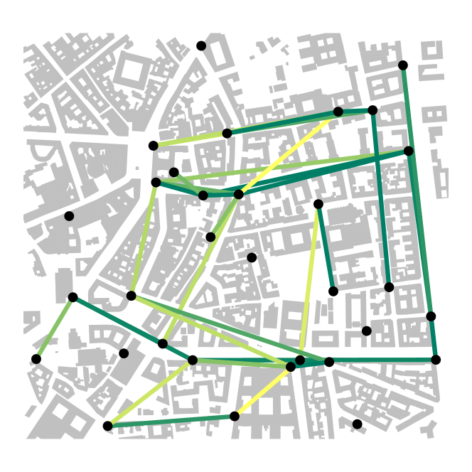
Figure 3: Map showing one of the four realistic networks in Milan, with density 45 gNBs/km². IAB-nodes are in black, and feasible backhaul links have a color gradient corresponding to their capacity (yellow for low capacity and green for high capacity).

V-A Topological Constraints

We divide the set of edges in $R$ disjoint sets, and impose that every tree rooted in an IAB-donor must use edges coming from only one out of $R$ sets, while every IAB-node must belong to at least $R$ trees. If $R=2$, there are two separate trees that serve each IAB-node $i$: if one edge fails in one tree and $i$ remains isolated, the second tree can be used to serve IAB-node $i$. This results in $R$ disjoint sets of edges, however we may have more trees, because the topological constraints and the availability of edges may make it impossible to have only $R$ trees. Each tree will have disjoint edges from each other tree, and each IAB-node will have $R$ parents, belonging to $R$ different trees rooted in two different IAB-donors. Figure 2 shows an example of an optimized topology when $D=3$ and $R=2$. The optimization creates two separate edge-set, represented using two colors. The optimization yields 3 IAB-donors out of 18 total gNBs (thus 15 IAB-nodes), and each IAB-donor is the root of a tree using edges coming only from one set. Every IAB-node has two parents connected with links using two distinct colors. As a consequence, if one edge fails and an IAB-node can not reach the IAB-donor at the root of the tree using the blue edge-set, it can still reach a IAB-donor using the tree made of orange edges.

The binary variable $u_{i,l,k}$ is set to 1 if IAB-node $i$ is at distance $l$ from the donor that is the root of a tree with edges in the sub-set $k\in[1,\ldots R]$. The binary variable $P_{i,j,k}$ is set to 1 if the edge from $i$ to $j$ is active in a tree that belongs to sub-set $k$. The optimization minimizes the total number of donors:

$$\text{objective:}\quad\text{min}\sum_{i\in\mathcal{N}_{v}}\sum_{k=1}^{R}u_{i,0,k},$$ (6)

under the following constraints:

$$\sum_{l=0}^{D}u_{i,l,k}=1-\sum_{r\neq k}u_{i,0,r}\quad\forall i,\forall k$$ (7)

$$\sum_{k}u_{i,0,k}\leq 1\quad\forall i$$ (8)

$$\sum_{i\in\mathcal{N}_{v}}P_{i,j,k}=1-\sum_{r}u_{j,0,r}\quad\forall j,k$$ (9)

$$\sum_{j\in\mathcal{N}_{v}}P_{i,j,k}<\delta\quad\forall i,k$$ (10)

$$P_{i,j,k}\leq 1-u_{j,l,k}+u_{i,l-1,k}\quad\forall i,j,k\quad\forall l\in\{1\ldots D\}$$ (11)

$$P_{i,j,k}\leq e_{i,j}\quad\forall i,j,k$$ (12)

$$\sum_{k}P_{i,j,k}+\sum_{k}P_{j,i,k}\leq 1\quad\forall i,j.$$ (13)

Eq. 7 imposes that every gNB must belong to at least one tree per edge-set $k$, unless it is an IAB-donor, which is the root of exactly one tree; Eq. 8 imposes that each IAB-donor must be the root of a single tree; Eq. 9 imposes that one IAB-donor of a certain tree has no incoming edges, and other nodes have one (thus it is a tree topology); Eq. 10 imposes the maximum out-degree; Eq. 11 imposes consistency on paths, hop by hop, that is, in a certain tree $k$ if a link connecting IAB-node $i$ to IAB-node $j$ is active, then the distance of IAB-node $i$ equals the distance of IAB-node $j$ minus one; Eq. 12 imposes that only existing links can be used; Eq. 13 imposes that every edge is used only in one direction and only in one tree. This last equation produces trees that are edge-disjoint.

There is always one trivial acceptable solution in which all gNBs are IAB-donors and the number of variables scales as $R|\mathcal{N}_{v}|^{2}$ as it is dominated by the dimension of $P_{i,j,k}$.

V-B Flow Constraints

We now introduce the flow-based constraints, implemented as a set of new equations on top of the topology-based ones, thus producing a topology and flow-based model. The flow-based model introduces three new sets of parameters, which are $d_{i}$ (the flow demand for IAB-node $i$), $C$ (the total maximum outgoing flow for an IAB-donor), and $L_{i,j}$ (the link capacity of $e_{i,j}$). It also introduces two new sets of variables. $f_{i,j,h,k}$ represents the flow destined to IAB-node $h$ passing through edge $e_{i,j}$ belonging to edge-set $k$. This is required because even if edges can not belong to more than one tree, the flow constraints need to be guaranteed in each edge and in every tree. $a_{i,j}$ is a real value in $[0,1]$ that represents the fraction of time link $e_{i,j}$ is used. As each node $j$ has a single radio for access and backhaul, it becomes necessary to impose a constraint on the total number of active links for $j$, modeled through variable $a_{i,j}$. If $j$ is connected to, for example, node 1 in upstream and node 2 in downstream, then $a_{1,j}+a_{2,j}\leq 1$.

The flow constraints are set as follows:

$$f_{i,j,i,k}=0\quad\forall\;i,j,k$$ (14)

$$\sum_{h}\sum_{j}f_{i,j,h,k}-\sum_{h\neq i}\sum_{j}f_{j,i,h,k}\leq C\sum_{k}u_{i,0,k}\quad\forall i,k$$ (15)

$$\sum_{j}f_{j,i,i,k}\geq(1-\sum_{h}u_{i,0,h})d_{i}\quad\forall i,k$$ (16)

$$a_{i,j}\leq\sum_{k}P_{i,j,k}\quad\forall\;i,j$$ (17)

$$\sum_{i}\sum_{h}\sum_{k}f_{i,j,h,k}\leq\sum_{i}L_{i,j}a_{i,j}\forall j$$ (18)

$$\sum_{h}\sum_{k}f_{i,j,h,k}\leq a_{i,j}L_{i,j}\quad\forall i,j$$ (19)

$$f_{i,j,h,k}\leq L_{i,j}P_{i,j,k}\quad\forall i,j,h,k$$ (20)

Here, Eq. 14 prevents self-loops in the flow graph, Eq. 15 imposes flow conservation for all IAB-nodes and all edge-set, except for donors that can output a flow $C$. Note that the real flow outgoing node $i$ is capped in every link by Eq. 19, so $C$ is just an arbitrary non zero upper bound that makes the equation formally correct, and it can model the bit-rate available on the wired link. Eq. 16 imposes that every IAB-node receives at least the amount of flow corresponding to its demand; Eq. 17 imposes that the usage on a link must be zero if the link is not chosen by the topology optimization; Eq. 18 imposes that an IAB-node can not receive in input more flow that what all its incoming link allow; similarly Eq. 19 imposes that flow on a link does not exceed its allocated capacity. Eq. 20 imposes that if an edge is not assigned to tree $k$ the corresponding flow in tree $k$ is zero. The objective function is Eq. 6, as these conditions only impose more constraints on the IAB-donors, with still a trivial solution with all gNBs as IAB-donors.

The cost associated with the model is the added complexity: the number of variables scales as $|\mathcal{N}_{v}|^{3}$ as it is dominated by the dimension of $f_{i,j,h}$. However, since every IAB-node has only one parent if the capacity of one incoming link to IAB-node $j$ is lower than the demand of IAB-node $j$ ($L_{i,j}<d_{j}$), we can set $e_{i,j}=0$ as that link cannot serve the demand of $d_{j}$. This allows us to prune some edges in $\mathcal{E}_{v}$ before running the optimization.

Finally, while our model is designed for a greenfield deployment, in which the operator is planning the network from scratch, it can also be used in a brownfield deployment in which some IAB-donors are already connected to the core with a fiber connection. The only required change in the model is the need to force some of the $u_{i,0,k}$ variables to be constant set to 1. This is important because we can use the optimization for both new networks, or to upgrade or dynamically control existing ones, as shown in Section VII. With a similar reasoning, if some of the locations of the gNBs is preferable than others, for instance if the cost of connecting it with fiber is smaller, the objective function can be modified so that every gNB has a different cost and not a simple unitary cost as in Eq. 6.

The whole problem is based on a multi-commodity flow problem merged with a shortest path multi-tree problem. There is however a key difference, the number and position of sources of the commodity are not decided a priori, but must be decided by the optimization. To the best of our knowledge, this specific problem has not been so far formulated. The problem is clearly non-polynomial because it mixes the multi-commodity flow with a combinatorial minimization of all the possible set of sources of the commodity. We also give the network designer the freedom to choose a maximum out the degree of and the distance from the IAB-donors. The second parameter in particular will affect the network delay, so it is important that the operator can define it based on the specific applications that must be supported.

VI Numerical Results

In this section, we report results on the feasibility and the effectiveness of the proposed optimization, leveraging the resilient and non-resilient versions of the flow optimization problem. We use as a metric the fraction $\rho$ of IAB-donors in the network, which is the ratio between the value of the objective function and the total size of the network $|\mathcal{N}_{v}|$:

$$\rho=\frac{\sum_{i\in\mathcal{N}_{v}}\sum_{k=1}^{R}u_{i,0,k}}{|\mathcal{N}_{v}|}.$$

First, we consider synthetic random graphs, to verify the feasibility of our approach in a controlled scenario, and then realistic graphs generated from open data of four European cities.

VI-A Synthetic Graphs

The synthetic graphs are generated by placing nodes in random positions in a 2D area, with an average density of 45 gNBs/km², which achieves 95% coverage of the outdoor urban areas [27]. We vary the area to deploy 15, 30, and 45 gNBs. The demand is estimated with Eq. 1, assuming a coverage radius of 100 m. We use the 3GPP TR 38.901 technical report for modeling both the probability of LoS between two gNBs and the path loss [37]. We thus do not explicitly model obstacles, and obtain networks with an edge density substantially higher than in real settings. We compute the link capacity as described in Section IV-B, using the parameters in Table I with 1 and 2 MIMO layers $\Lambda$. Execution times are evaluated on a 16 cores server (Intel Xeon Gold 6342 CPU @ 2.80GHz), with 64GB of RAM using the Gurobi solver with 30 randomly generated graphs for each number of gNBs. After 48 hours the solver was stopped, and for those runs that did not reach the optimal value, we report the upper bound distance from the optimum.

Figure 4 shows the ratio $\rho$ between IAB-donors and total number of gNBs in the simulation. The two leftmost plots (a, b) report the results with only one tree ($R=1$), while plots (c, d) report the failure resilient model ($R=2$), both with $\Lambda=1$, $\Lambda=2$. As a general trend, higher $\Lambda$ and lower $R$ lead to lower $\rho$. This is expected since with a higher capacity per link the backhaul network can transport more traffic to a smaller number of donors, while redundancy requires more independent trees and thus more donors. Increasing $|\mathcal{N}_{v}|$ enlarges the space of possible results and can lead to a further reduction of the number of required IAB-donors. For the most challenging configuration ($\Lambda=1,R=2$), the median value of $\rho$ ranges from 0.66 to 0.6, which means that we can save up to 40% of the donors. Savings increase to up to 60% with $\Lambda=2,R=2$ and 45 gNB/km², which means that 27 gNBs out or 45 do not need to be connected with a fiber cable.

The failure resilient topology imposes the strong condition that all flow is conserved and there is no performance degradation upon the failure of a link. If we relax this condition, and set $R=1$, we can further reduce the number of IAB-donors down to 37% (45 gNBs, $\Lambda=1$) and 23% (45 gNBs, $\Lambda=2$), introducing a non-zero probability of network outage. This does not necessarily imply that the failure of one link disconnects some UE, but it could produce a certain performance degradation. Models can be tailored to provide a trade-off between these two approaches, obtaining $\rho$ close to the ones generated with $R=1$ with a predictable performance penalty in case of failure.

(a) $\Lambda=1,\,R=1$

(b) $\Lambda=2,\,R=1$

(c) $\Lambda=1,R=2$

(d) $\Lambda=2,R=2$

Figure 4: Box-plots of the fraction of donors $\rho$ for the synthetic topologies, with different MIMO configuration ($\Lambda=1$, $\Lambda=2$), the single tree model ($R=1$) and the failure resistant model ($R=2$). The box plot show the median, 25% and 75% quartile and 1.5*IQR (inter quantile range) whiskers.

For solver execution runs that lasted at most 48 hours, a guaranteed optimal solution has been identified in 67% of the cases. In the remaining ones, the upper bound of the distance of $\rho$ from the global optimum is on average 6.3%. This is perfectly compatible with the network planning use case.

VI-B Real-world Graphs

The realistic graphs were generated for 4 cities (Florence and Milan in Italy, Barcelona in Spain, and Luxembourg city), in an area of about one km², as in Fig. 3.

For each scenario, we use densities of 30, 45, and 60 gNBs/km²; run the placement heuristic to position the gNBs; and compute the capacity as described in Section IV-B. Some gNBs are placed out of range from all others, and thus removed from the graph.

(a) $\Lambda=1,\;R=1$

(b) $\Lambda=2,\;R=1$

(c) $\Lambda=1,\;R=2$

(d) $\Lambda=2,\;R=2$

Figure 5: Fraction of donors $\rho$ for the realistic topologies, with different MIMO configuration ($\Lambda=1$, $\Lambda=2$), the single tree model ($R=1$) and the failure resilient model ($R=2$).

Figure 5 confirms results obtained in the synthetic scenarios, i.e., also in the realistic scenario fewer IAB-donors are required as the density increases. In the realistic topologies the presence of obstacles makes the the topology less dense, and the distribution of users more concentrated, eventually this reduces the complexity of the problem and we can complete the optimization even with 60 gNBs/km², and in some configurations $\rho$ is lower than 20% (Fig. 5(b)). Only in 4 cases over 48 runs the optimization did not reach the optimal value, and in those 4 cases the upper bound of the distance of $\rho$ from the global optimum is on average 6%.

Overall our results confirm that in both synthetic and real-world scenarios our optimization scheme is reliable and produces resilient topologies that can save a large number of IAB-donors, reducing the capital expenditure of fiber backhaul.

VII Backhaul rApp Prototype and Validation

In this section, we discuss the integration of our methodology within the O-RAN framework, allowing operations and management of real-world networks. We implement a prototype rApp running in the Non-RT RIC, which processes a network made of $R=2$ trees (a primary and a back-up one) and gracefully handles the failure of a link by reconfiguring all the gNBs to switch from their primary tree to the backup one. We validate the rApp using OpenAirInterface on Colosseum.

The application is initialized with the multitree topology obtained in the network planning phase. Once the network is set-up and running, the rApp maintains an updated representation of the IAB network using specific messages (HeartBeats, Performance Reports, and Fault Events) exchanged with the RAN through the O-RAN O1 Interface (see Fig. 1). Upon the failure of a radio link between IAB-nodes, the upstream node, still connected to the core, detects the Radio Resource Control (RRC) failure and sends a Failure Event message to the RIC through the O1 interface. The rApp reconfigures the network by updating the upstream connectivity of the IAB-node (which may require a reset of the stack in the OAI prototype). It also updates all the IAB-nodes downstream since they need to reconnect to the network core using a new path. Finally, it reconfigures routing within the core network to reflect the new downstream IAB-nodes topology.

VII-A Validation on Colosseum

Currently, the OAI stack does not support handover between different upstream nodes, so it introduces long delays and performance fluctuations due to the need to restart the protocol stack. For this reason, our goal is not to provide an accurate performance analysis, but to demonstrate that our approach can be implemented in a real network. We have set up a representative IAB-network topology, shown in Fig. 6, comprising two IAB-donors, two IAB-nodes and twenty UEs. Each IAB-node is connected to a different IAB-donor, and a feasible (but unused) link is available between the two IAB-nodes. Note that we assume gNBs have a secondary communication channel for their management through the O1 interface, possibly using the sub-GHz bands in order to be less subject to blockage [38].

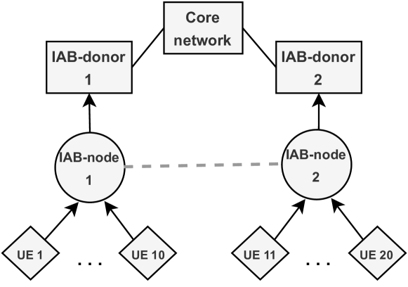
Figure 6: IAB topology including the Core network, two IAB-donors, two IAB-nodes and 20 UEs. Black arrows indicate the normal topology and the grey dotted line indicates the backup link between the two IAB-nodes.

In our experiment, once the rApp initializes the whole network, all UEs and all IAB-nodes start exchanging Internet Control Message Protocol (ICMP) traffic with a server in the core network, routed through the parent IAB-node or donor. Then, we emulate the failure of the link between IAB-node 2 and its donor. This triggers the transmission of a Fault Event message to the rApp, which in turn triggers the reconfiguration of IAB-node 2, which will connect to IAB-node 1 to reach the core. Since the current implementation of IAB for Colosseum and OAI creates end-to-end tunnels from UEs to the core network [11], the UEs attached to IAB-node 2 must also be reconfigured. Moreover, the rApp reconfigures the 5G core, so that the backward path to the UEs is also restored.

Figure 7 shows how the Round Trip Time (RTT) of the transmitted packets is affected during and after the reconfiguration of the network. We average the RTT on a rolling window of 10 s and across UEs for each node. At $t=0$ both IAB-nodes report a RTT of roughly 10 ms and their UEs measure an RTT of roughly 24 ms, which accounts for one more wireless hop and some switching time. At time $t=19$ s, we induce the failure of the link between IAB-node 2 and IAB-donor 2, which interrupts the successful transmission of the ICMP packets and triggers the reconfiguration of the network from the rApp. The reconfiguration of the OAI stack takes roughly 15 s, albeit being fully automated. Around second $t=35$ s, IAB-node 2 is able to reach the core again, with an average RTT of 22 ms, due to the additional hop. At that point, also the software-defined UEs stack restarts, with their RTT increased to an average of 47 ms, corresponding to 3 hops of distance to the core and two switching delays.

Despite the current state of OAI affects the performance of the reconfiguration, this experiment fully confirms the viability of our approach in a real-world network scenario based on the O-RAN specifications.

Figure 7: RTT from the IAB-nodes and the UEs before, during, and after the link failure. The vertical lines indicate the time of fault and the time of the two recoveries.

VIII Conclusions

Next-generation wireless networks require optimized and intelligent management for their complex backhaul configurations, mixing wired and wireless components. This paper proposed a novel toolchain to plan a mobile backhaul, based on open data to model 3D scenarios, optimization strategies to plan the network, and an O-RAN rApp for dynamic network control. We have shown that the optimization problems can be solved for realistic networks of density up to 60 gNBs/km², and this can lead to the reduction of a substantial number of fiber drops. The models are fully configurable in terms of depth of the IAB tree and required robustness, and can be used in greenfield or brownfield scenarios, and the approach has been prototyped in a realistic O-RAN-based network environment.

References

- [1] E. Yaacoub and M.-S. Alouini, “A Key 6G Challenge and Opportunity—Connecting the Base of the Pyramid: A Survey on Rural Connectivity,” Proceedings of the IEEE, vol. 108, no. 4, April 2020.
- [2] W. Saad, M. Bennis, and M. Chen, “A Vision of 6G Wireless Systems: Applications, Trends, Technologies, and Open Research Problems,” IEEE Network, vol. 34, no. 3, May 2020.
- [3] T. S. Rappaport, S. Sun, R. Mayzus, H. Zhao, Y. Azar, K. Wang, G. N. Wong, J. K. Schulz, M. Samimi, and F. Gutierrez, “Millimeter wave mobile communications for 5g cellular: It will work!” IEEE Access, vol. 1, 2013.
- [4] ITU-R, “Guidelines for evaluation of radio interface technologies for IMT-2020,” Report ITU-R M.2412-0. [Online]. Available: https://www.itu.int/dms\_pub/itu-r/opb/rep/R-REP-M.2412-2017-PDF-E.pdf
- [5] C. Madapatha, B. Makki, C. Fang, O. Teyeb, E. Dahlman, M.-S. Alouini, and T. Svensson, “On Integrated Access and Backhaul Networks: Current Status and Potentials,” IEEE Open Journal of the Communications Society, vol. 1, 2020.
- [6] M. Polese, M. Giordani, T. Zugno, A. Roy, S. Goyal, D. Castor, and M. Zorzi, “Integrated access and backhaul in 5G mmWave networks: Potential and challenges,” IEEE Communications Magazine, no. 3, 2020.
- [7] V. Raghavan, V. Podshivalov, J. Hulten, M. A. Tassoudji, A. Sampath, O. H. Koymen, and J. Li, “Spatio-Temporal Impact of Hand and Body Blockage for Millimeter-Wave User Equipment Design at 28 GHz,” IEEE Communications Magazine, vol. 56, no. 12, December 2018.
- [8] C. Saha and H. S. Dhillon, “Millimeter wave integrated access and backhaul in 5g: Performance analysis and design insights,” IEEE Journal on Selected Areas in Communications, vol. 37, no. 12, 2019.
- [9] P. Fiore, E. Moro, I. Filippini, A. Capone, and D. D. Donno, “Boosting 5G mm-Wave IAB Reliability with Reconfigurable Intelligent Surfaces,” in IEEE Wireless Communications and Networking Conference (WCNC), April 2022.
- [10] S. Gopalam, S. V. Hanly, and P. Whiting, “Distributed and Local Scheduling Algorithms for mmWave Integrated Access and Backhaul,” IEEE/ACM Transactions on Networking, vol. 30, no. 4, Aug 2022.
-
[11]
E. Moro, G. Gemmi, M. Polese, L. Maccari, A. Capone, and T. Melodia, “Toward
Open Integrated Access and Backhaul
with O-RAN,” in 21st Mediterranean Communication and Computer Networking Conference (MedComNet 2023). IEEE, 2023. - [12] M. Polese, L. Bonati, S. D’Oro, S. Basagni, and T. Melodia, “Understanding O-RAN: Architecture, interfaces, algorithms, security, and research challenges,” IEEE Communications Surveys & Tutorials, 2023.
- [13] L. Bonati, P. Johari, M. Polese, S. D’Oro, S. Mohanti, M. Tehrani-Moayyed, D. Villa, S. Shrivastava, C. Tassie, K. Yoder, A. Bagga, P. Patel, V. Petkov, M. Seltser, F. Restuccia, A. Gosain, K. R. Chowdhury, S. Basagni, and T. Melodia, “Colosseum: Large-Scale Wireless Experimentation Through Hardware-in-the-Loop Network Emulation,” in IEEE International Symposium on Dynamic Spectrum Access Networks (DySPAN), 2021.
- [14] B. Tezergil and E. Onur, “Wireless Backhaul in 5G and Beyond: Issues, Challenges and Opportunities,” IEEE Communications Surveys & Tutorials, vol. 24, no. 4, 2022.
- [15] J. Y. Lai, W.-H. Wu, and Y. T. Su, “Resource allocation and node placement in multi-hop heterogeneous integrated-access-and-backhaul networks,” IEEE Access, vol. 8, 2020.
- [16] C. Madapatha, B. Makki, A. Muhammad, E. Dahlman, M.-S. Alouini, and T. Svensson, “On Topology Optimization and Routing in Integrated Access and Backhaul Networks: A Genetic Algorithm-Based Approach,” IEEE Open Journal of the Communications Society, vol. 2, 2021.
- [17] M. Pagin, T. Zugno, M. Polese, and M. Zorzi, “Resource Management for 5G NR Integrated Access and Backhaul: A Semi-Centralized Approach,” IEEE Trans. on Wireless Communications, vol. 21, no. 2, Feb. 2022.
- [18] D. Yuan, H.-Y. Lin, J. Widmer, and M. Hollick, “Optimal and Approximation Algorithms for Joint Routing and Scheduling in Millimeter-Wave Cellular Networks,” IEEE/ACM Transactions on Networking, vol. 28, no. 5, Oct. 2020.
- [19] Y. Zhang, V. Ramamurthi, Z. Huang, and D. Ghosal, “Co-Optimizing Performance And Fairness Using Weighted Pf Scheduling And Iab-Aware Flow Control,” in IEEE Wireless Communications and Networking Conference (WCNC), May 2020.
- [20] S. Gopalam, S. V. Hanly, and P. Whiting, “Distributed and local scheduling algorithms for mmwave integrated access and backhaul,” IEEE/ACM Transactions on Networking, vol. 30, no. 4, 2022.
- [21] Z. Ma, B. Li, Z. Yan, and M. Yang, “QoS-Oriented joint optimization of resource allocation and concurrent scheduling in 5G millimeter-wave network,” Computer Networks, vol. 166, Jan. 2020.
- [22] S. Zhang, X. Xu, M. Sun, X. Tao, and C. Liu, “Joint Spectrum and Power Allocation in 5G Integrated Access and Backhaul Networks at mmWave Band,” in IEEE 31st Annual International Symposium on Personal, Indoor and Mobile Radio Communications (PIMRC), Aug. 2020.
- [23] M. N. Islam, S. Subramanian, and A. Sampath, “Integrated access backhaul in millimeter wave networks,” in IEEE Wireless Communications and Networking Conference (WCNC), 2017.
- [24] M. N. Islam, N. Abedini, G. Hampel, S. Subramanian, and J. Li, “Investigation of performance in integrated access and backhaul networks,” in IEEE Conference on Computer Communications Workshops (INFOCOM WKSHPS), 2018.
- [25] J. Mcmenamy, A. Narbudowicz, K. Niotaki, and I. Macaluso, “Hop-Constrained mmWave Backhaul: Maximising the Network Flow,” IEEE Wireless Communications Letters, vol. 9, no. 5, May 2020.
- [26] C. Villien, N. Deparis, V. Mannoni, and S. De Rivaz, “Prediction of toa-based localization accuracy using crlb and 3d buildings with field trial validation,” in Joint European Conference on Networks and Communications and 6G Summit (EuCNC/6G Summit), 2022.
- [27] G. Gemmi, R. Lo Cigno, and L. Maccari, “On cost-effective, reliable coverage for los communications in urban areas,” IEEE Transactions on Network and Service Management, vol. 19, no. 3, 2022.
- [28] A. Al-Hourani, “On the probability of line-of-sight in urban environments,” IEEE Wireless Communications Letters, vol. 9, no. 8, 2020.
- [29] Open Street Map 3D buildings. [Online]. Available: https://osmbuildings.org/
- [30] O-RAN Working Group 2, “O-RAN Non-RT RIC Architecture 1.0,” O-RAN.WG2.Non-RT-RIC-ARCH-TS-v01.00 Technical Specification, July 2021.
- [31] C. Madapatha, B. Makki, H. Guo, and T. Svensson, “Constrained Deployment Optimization in Integrated Access and Backhaul Networks,” in IEEE Wireless Communications and Networking Conference (WCNC), March 2023.
- [32] H. Ling, R.-C. Chou, and S.-W. Lee, “Shooting and bouncing rays: calculating the rcs of an arbitrarily shaped cavity,” IEEE Transactions on Antennas and Propagation, vol. 37, no. 2, 1989.
- [33] M. Lecci, P. Testolina, M. Polese, M. Giordani, and M. Zorzi, “Accuracy versus complexity for mmwave ray-tracing: A full stack perspective,” IEEE Transactions on Wireless Communications, vol. 20, no. 12, Dec 2021.
- [34] F. Kaltenberger, A. P. Silva, A. Gosain, L. Wang, and T.-T. Nguyen, “OpenAirInterface: Democratizing innovation in the 5G era,” Computer Networks, no. 107284, May 2020.
- [35] OpenAirInterface SNR-MCS tables. [Online]. Available: https://gitlab.eurecom.fr/oai/openairinterface5g/-/tree/develop/openair1/SIMULATION/NR_PHY/BLER_SIMULATIONS/AWGN
- [36] 3GPP, “NR; User Equipment (UE) radio access capabilities,” TS 38.306 V17.5.0, 2023.
- [37] 3GPP, “Study on channel model for frequencies from 0.5 to 100 GHz,” Technical Report (TR) 38.901, Jun. 2018.
- [38] J.-H. Kwon, B. Lim, and Y.-C. Ko, “Resource Allocation and System Design of Out-Band Based Integrated Access and Backhaul Network at mmWave Band,” IEEE Transactions on Vehicular Technology, vol. 71, no. 6, June 2022.