Joint Modeling of Quasar Variability and Accretion Disk Reprocessing using Latent Stochastic Differential Equations

Abstract

Quasars are bright active galactic nuclei powered by the accretion of matter around supermassive black holes at the center of galaxies. Their stochastic brightness variability depends on the physical properties of the accretion disk and black hole. The upcoming Rubin Observatory Legacy Survey of Space and Time (LSST) is expected to observe tens of millions of quasars, so there is a need for efficient techniques like machine learning that can handle the large volume of data. Quasar variability is believed to be driven by an X-ray corona, which is reprocessed by the accretion disk and emitted as UV/optical variability. We are the first to introduce an auto-differentiable simulation of the accretion disk and reprocessing. We use the simulation as a direct component of our neural network to jointly model the driving variability and reprocessing to fit simulated LSST 10-year quasar light curves. The driving variability is reconstructed using a latent stochastic differential equation, a physically motivated, generative deep learning method that can model continuous-time stochastic dynamics. By embedding these physical processes into our network, we achieve a model that is more robust and interpretable. We also use transformers to scale our model to tens of millions of parameters. We demonstrate how our model outperforms a Gaussian process regression baseline and can infer accretion disk parameters and time delays between wavebands, even for out-of-distribution driving signals. Our approach provides a powerful and scalable framework that can be adapted to solve other inverse problems in multivariate time series with irregular sampling.

1 Introduction

Active galactic nuclei (AGN) are thought to be powered by the accretion of matter around supermassive black holes at the center of galaxies (Salpeter, 1964; Zel’dovich, 1964). Quasars are bright AGN with unobscured accretion disks and are some of the brightest objects in the Universe. They are observable at extreme cosmological distances making them powerful probes of the early Universe (Mortlock et al., 2011; Bañados et al., 2018). Quasars are also thought to play an important role in galaxy evolution (Franceschini et al., 1999; Kauffmann & Haehnelt, 2000; Hoshi et al., 2024). The variability of quasar brightnesses has been studied since their discovery (Greenstein, 1963; Hazard et al., 1963; Matthews & Sandage, 1963; Oke, 1963; Schmidt, 1963). These brightness variations are related to the physical properties of the black hole and accretion disk that powers them. Investigating the physics governing quasar light curves offers valuable insights into our understanding of cosmology (Khadka & Ratra, 2020; Czerny et al., 2023).

The UV/optical variability of quasars is most often modeled as an X-ray driving variability source corona that illuminates the accretion disk (Cackett et al., 2007). The reprocessing of the driving variability to the UV/optical emitting regions of the accretion disk is represented by the transfer function and introduces wavelength dependent time lags (Blandford & McKee, 1982), ranging from less than a day for small supermassive black holes ($\sim 10^{7}M_{\odot}$) to several tens of days ($\sim 10^{10}M_{\odot}$). These time lags can be measured through continuum reverberation mapping of UV/optical light curves to probe the relative size scales of the emitted regions, and are interconnected to properties of the accretion disk and black hole (Cackett et al., 2021; Jha et al., 2022; Wang et al., 2023).

Studies of quasar variability have found accretion disk sizes to be larger than the predictions of the thin-disk model by a factor of $\sim$2–4 (Mudd et al., 2018; Guo et al., 2022; Jha et al., 2022). This is also consistent with accretion disk size measurements found using gravitational microlensing (Poindexter et al., 2008; Poindexter & Kochanek, 2010; Blackburne et al., 2015; Muñoz et al., 2016; Morgan et al., 2018). New measurements and methods are needed to test accretion disk models and enhance our understanding of the physical processes governing quasar emissions.

Upcoming wide-field surveys such as the Rubin Observatory Legacy Survey of Space and Time (LSST) will observe an unprecedented quantity of data. The LSST main survey will cover 18,000 $\deg^{2}$ and is projected to monitor tens of millions of quasars over a ten year period with six UV/optical bandpass filters (ugrizy) at 55–185 samplings per band or around 800 total visits across the ten years out to redshift of $z\sim 7.5$ (Collaboration et al., 2009; Prša et al., 2023). A smaller sky area of 200 $\deg^{2}$ known as the Deep Drilling Fields is expected to detect 40,000 additional ultrafaint AGN at higher cadences of about 1,000 samplings per band (Brandt et al., 2018). Machine learning (ML) algorithms are well suited to analyze the vast amounts of data expected from LSST and other wide-field surveys. The quasar light curves from LSST pose challenges for traditional machine learning techniques due being stochastic, multivariate, having irregular cadences spread across the different bands, long seasonal gaps without observations, and photometric noise.

The UV/optical variability of quasars is most commonly modeled using Gaussian process regression (GPR). In this framework, quasar light curves are fit with a specific kernel, for example the kernel associated with the damped random walk (DRW) process (Zu et al., 2013). The optimized kernel parameters have been empirically shown to be related to properties of the quasar such as the black hole mass (MacLeod et al., 2010; Suberlak et al., 2021).

The codebase JAVELIN (Zu et al., 2011, 2016) uses a DRW kernel with top hat transfer functions to simultaneously model the variability and time delays. The bluest band is taken as the effective driving variability source and fit using the DRW, and the top hat transfer functions are used to measure the time delays between the other bands. This method relies on Markov Chain Monte Carlo (MCMC) to sample the DRW kernel and transfer function parameters. By default, JAVELIN measures the time delays but does not directly extract physical properties of the quasar. Simple parametric models can be fit to the time delay measurements as a secondary step to measure the accretion disk size and sometimes the temperature profile, although it is most often fixed to the thin-disk case. In Mudd et al. (2018), JAVELIN was modified to measure the accretion disk size directly by fixing the time delays to the thin-disk model.

The codebase CREAM (Starkey et al., 2015) is similar to JAVELIN but uses the thin-disk transfer functions directly instead of top hats. Instead of treating the bluest band as the effective driving variability, CREAM explicitly reconstructs the driving variability by modeling it as a Fourier series. MCMC is used to optimizes the Fourier components of the driving variability and the accretion disk parameters, and both the driving variability and transfer function kernels are reconstructed. In theory, CREAM can recover the product of the black hole mass and accretion rate, $M\dot{M}$, and the inclination angle, although the inclination cannot be recovered without very high-fidelity data. For example, it was used in Fausnaugh et al. (2018) to model two Seyfert 1 galaxies to measure $M\dot{M}$ and to constrain the inclination for one galaxy.

Both JAVELIN and CREAM rely on computationally expensive MCMC sampling, which may be infeasible to apply to the tens of millions of quasar light curves expected from LSST. In addition, the DRW kernel in JAVELIN is only fit with respect to the bluest band, however the information in each band is highly correlated to the other bands so jointly modeling the light curves and time delays would show improvements in performance. This is especially the case for sparsely and irregularly sampled cadences like what is expected from LSST. Optical/UV light curves have also been shown to significantly deviate from a DRW, so a more flexible fitting method would be beneficial. CREAM does jointly model the driving variability and transfer functions; however, the driving variability is modeled as a Fourier series. This may become infeasible for long light curves like what we expect from LSST, since the driving signal is expected to be stochastic across many time scales. Ideally our methods would be able to learn from features across an entire sample of light curves. For example, there is additional information in the mean brightnesses of each band could be combined with time delay measurements to better estimate accretion disk parameters and breaking some of the degeneracies. Our machine learning approach improves upon all these areas.

Machine learning methods have been used to model quasar variability using various methods. Tachibana et al. (2020) used a recurrent auto-encoder to model quasar variability and found it to perform better than a DRW model when applied to real data. Sá nchez-Sáez et al. (2021) used a recurrent variational auto-encoder for anomaly detection to find changing-look AGNs. Park et al. (2021) introduced a method to simultaneously reconstruct quasar light curves and predict accretion disk parameters using attentive neural processes. Čvorović Hajdinjak et al. (2022) introduced conditional neural processes to model quasar variability. Sheng et al. (2022) applied stochastic recurrent neural networks to reconstruct simulated LSST light curves. Danilov et al. (2022) developed a neural inference Gaussian processes method, outperformed standard GPR. Li et al. (2024) demonstrated how simulation based inference could be used to predict accretion disk parameters. For microlensed quasar light curves, Vernardos & Tsagkatakis (2019) used a convolutional neural network to measure the accretion disk size and temperature profile in simulated light curves, and Best et al. (2024a) predicted the black hole mass, inclination angle, and impact angle. Fagin et al. (2024a) developed a method of predicting high magnification microlensing events through real time classification with simulated LSST light curves using a recurrent neural network.

Fagin et al. (2024b) introduced latent stochastic differential equations (SDEs) as a method to reconstruct simulated LSST-like quasar light curves and simultaneously predict accretion disk and variability parameters. Latent SDEs are a type of generative neural network that can model continuous-time stochastic dynamics (Li et al., 2020). They are physically motivated by the fact that UV/optical quasar variability is often modeled by SDEs such as the DRW or higher order continuous-time autoregressive moving-average (CARMA) processes (Yu et al., 2022). Latent SDEs can be viewed as infinite-dimensional variational autoencoders (VAEs; Kingma & Welling, 2013; Rezende et al., 2014) with an SDE-induced process as their latent state. Fagin et al. (2024b) found the deep learning method to be superior to a multitask GPR baseline in reconstructing LSST light curves. Their model also simultaneously performed parameter inference based on the context vector of the encoder as well as the latent vector of the SDE. They found they were able to predict the black hole mass, temperature slope, and inclination angle as well as the parameters of the DRW driving variability signal.

While the latent SDE method of Fagin et al. (2024b) is able to simultaneously reconstruct the light curve and perform parameter inference, the reconstructed light curve and parameter predictions do not necessarily correspond to the same time delays. In this work, we are the first to combine the light curve reconstruction and parameter inference into a self-consistent, unified framework. This is achieved by developing the first auto-differentiable simulation of the accretion disk and including it into the architecture of our machine learning model. Within our neural network, we use a latent SDE to generate the X-ray driving variability. We then predict the accretion disk parameters, which are converted to the corresponding transfer functions using our auto-differentiable simulation of the disk. The reconstructed driving variability is convolved with the transfer functions and then scaled to produce the mean best fit reconstruction of each observed UV/optical band. We also produce uncertainty on the mean prediction in our network to best reconstruct the driving variability and observed light curve. In addition, we predict the variability parameters of the driving signal and produce uncertainties on our inferred parameters. Furthermore, the network predicts the relative time delays between bands from the mean time delay of the reconstructed transfer functions, and their uncertainties are quantified by the network.

Recurrent inference machine (RIM; Putzky & Welling, 2017) has been used to solve inverse problems in several astrophysics applications (Morningstar et al., 2019; Modi et al., 2021; Adam et al., 2022; Rhea et al., 2023). Our goal in this work is to solve the blind deconvolution inverse problem of recovering the driving signal and transfer functions given the observations of our light curve. This is made particularly challenging given the stochastic nature of quasar variability and the fact that our observations are irregular and sparsely sampled which include long seasonal gaps of missing data. We use RIM in our network to iteratively improve upon the light curve reconstruction and accretion disk parameter estimation in our neural network.

In section 2, we describe how we build a realistic simulation of quasar light curves including an auto-differentiable version that is incorporated into our neural network. In section 3, we present our machine learning model architecture and training. In section 4, we give our results on our model’s performance on light curve reconstruction and parameter inference. In Section 5, we discuss the results of our network and its applicability to LSST, and Section 6 gives our concluding remarks. Throughout this work we assume a flat $\Lambda$CDM cosmology with $H_{0}=70$ $\text{km}\,\text{s}^{-1}\,\text{Mpc}^{-1}$, $\Omega_{m}=0.3$, and $\Omega_{\Lambda}=0.7$.

2 Light curve simulation

We train our neural network with realistic simulations of LSST ten year light curves. The reprocessing of the X-ray driving variability by the accretion disk to the UV/optical wavelength $\lambda$ is modeled by:

$$F_{\lambda}(t,\lambda)=\bar{F}_{\lambda}(\lambda)+\Delta F_{\lambda}(\lambda)\int_{0}^{\infty}X(t-\tau)\psi(\tau|\lambda)\text{d}\tau,$$ (1)

where $F_{\lambda}(t,\lambda)$ is the observed flux, $\bar{F}_{\lambda}(\lambda)$ is the mean flux, $\Delta F_{\lambda}(\lambda)$ is the amplitude of the variable flux, $X(t)$ is the normalized driving variability (mean zero and variance one), and $\psi(\tau|\lambda)$ is the transfer function kernel (Cackett et al., 2007; Starkey et al., 2015; Chan et al., 2024). Section 2.1 describes how we model the driving variability $X(t)$. Section 2.2 introduces our auto-differentiable model of the accretion disk reprocessing and transfer functions $\psi(\tau|\lambda)$. In section 2.3, we construct realistic spectrum from our accretion disk model using templates for the spectral lines, host galaxy flux, and extinction. We then integrate the spectrum across the filter response functions of each LSST band to get the mean flux and variability amplitude of each band $\bar{F}_{\lambda}(\lambda)$ and $\Delta F_{\lambda}(\lambda)$. Section 2.4 gives the parameter ranges for building our training set, and section 2.5 describes how the time series is degraded to mimic LSST observational cadences and noise.

2.1 Quasar Driving Variability Model

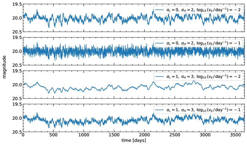
Figure 1: Example driving variability generated using the bending broken power-law power spectrum given in Equation (6) with different values for $\alpha_{L}$, $\alpha_{H}$, and $\nu_{b}$. Each driving variability has an asymptotic mean of 20 mag, asymptotic standard deviation of 0.1 mag, and redshift $z=0$.

UV/optical quasar variability is often modeled as a DRW, a type of Gaussian process also known as the Ornstein-Uhlenbeck process (Rasmussen & Williams, 2006; Zu et al., 2013). A DRW signal $X(t)$ is governed by the SDE:

$$dX(t)=-\frac{1}{\tau}X(t)\ dt+\sigma\sqrt{dt}\ \epsilon(t)+b\ dt$$ (2)

where $\epsilon(t)$ is a white noise process with a mean of zero and variance of one, $\tau$ is the characteristic timescale, $b$ is related to the mean of the process $\overline{X}=b\tau$, and $\sigma$ is related to the standard deviation defined by the asymptotic structure function $\text{SF}_{\infty}=\sigma\sqrt{\tau/2}$ (Kelly et al., 2009). The DRW can instead be characterized by its power spectral density (PSD) given by:

$$P(\nu)=\frac{4\tau\text{SF}_{\infty}^{2}}{1+(2\pi\tau\nu)^{2}},$$ (3)

for frequency $\nu$. This model is useful because GPR can be used to measure the variability parameters $\tau$ and $\text{SF}_{\infty}$ using the kernel of the Gaussian process:

$$k(\Delta t)=\text{SF}_{\infty}^{2}\,\exp\left(-\frac{\Delta t}{\tau}\right)$$ (4)

where $\Delta t$ are the time separation of two observations. The measured values of $\tau$ and $\text{SF}_{\infty}$ have been empirically shown to relate to properties of the accretion disk such as the black hole mass (MacLeod et al., 2010; Suberlak et al., 2021). More complex Gaussian processes have also been used such as higher order continuous-time autoregressive moving-average (CARMA) processes (Yu et al., 2022). These CARMA processes are the solution to higher order SDEs than the DRW given in Equation (2).

The X-ray driving variability is better modeled as a broken power-law PSD:

$$P(\nu)\propto\begin{cases}(\nu/\nu_{b})^{-\alpha_{L}},&\text{if }\nu<\nu_{b}\\ (\nu/\nu_{b})^{-\alpha_{H}},&\text{if }\nu>\nu_{b}\end{cases}$$ (5)

where $\nu_{b}$ is the break frequency between the lower power-law slope $\alpha_{L}$ and the higher power-law slope $\alpha_{H}$. This is not a Gaussian process, but the parameters of the broken power-law can be measured by analyzing the PSD. We use the bending broken power-law which is a continuous version of Equation (5) and defined as:

$$P(\nu)\propto\nu^{-\alpha_{L}}\left(1+\left(\frac{\nu}{\nu_{b}}\right)^{\alpha_{H}-\alpha_{L}}\right)^{-1},$$ (6)

which implies that $P(\nu)\propto\nu^{-\alpha_{L}}$ at low frequencies when $f\ll\nu_{b}$ and $P(\nu)\propto\nu^{-\alpha_{H}}$ when $f\gg\nu_{b}$. A form of the bending broken power-law has been extensively used to model the X-ray variability (i.e, McHardy et al., 2004; Uttley & McHardy, 2005; O’Neill et al., 2005; Summons, 2007; Markowitz, 2010; Sartori et al., 2019; Yang et al., 2022; Yuk et al., 2023; Czerny et al., 2023). In the special case where $\alpha_{L}=0$, $\alpha_{H}=2$, and $\nu_{b}=1/(2\pi\tau)$, the bended broken power-law recovers the PSD of the DRW in Equation (3). More often, the broken power-law for X-ray variability has measured $\alpha_{L}\sim 1$ and $\alpha_{H}\sim 3$. The parameters of the broken power-law have been shown to relate to properties of the accretion disk and black hole (Arevalo et al., 2023).

We can generate light curves from any PSD using the method of Timmer & Koenig (1995) by taking the inverse Fourier transform with randomized complex phases. This method has been used to generate X-ray variability with the bending broken power-law, for example in Czerny et al. (2023). We generate the driving variability at a length eight times larger than our desired signal and keep only a the initial desired length. This is to avoid the boundary conditions of the Fourier transform, and so we can set the asymptotic mean and standard deviation to the longer time series without bias (described in more detail in Section 2.3). We generate the driving variability at daily intervals and in magnitude so the flux is always positive.

The power spectrum in Equation (6) is in the rest frame of the quasar. We predict the break frequency in the observer frame to avoid degeneracies with the redshift. The posteriors of our break frequency and redshift can be combined after the fact to obtain the rest frame break frequency: $\nu_{b}^{\text{rest}}=(1+z)\nu_{b}^{\text{obs}}$, which should be what is correlated to physical properties of the accretion disk.

Example driving variability is given in Figure 1 from the bending broken power-law (Equation (6)). The top two panels have $\alpha_{L}=0$ and $\alpha_{H}=2$ making them equivalent to the DRW given by Equation (2). The bottom two panels have $\alpha_{L}=1$ and $\alpha_{H}=3$ which are more common values for modeling X-ray variability.

2.2 Auto-Differentiable Accretion Disk Model

Our goal is to use the accretion disk model to simulating our training set and as a component of our neural network. We simulate the accretion disk and transfer functions in PyTorch (Paszke et al., 2019), enabling automatic differentiation (Baydin et al., 2018), and allowing us to use the model with gradient based optimization in our neural network (i.e. we can use back propagation and gradient descent to update the weights of our neural network). The transfer functions $\psi(\tau|\lambda,\boldsymbol{\eta})$ are parameterized by a set of accretion disk and black hole parameters, given by the vector $\boldsymbol{\eta}$.

We use a modified version of the Novikov-Thorne (NT) model (Novikov & Thorne, 1973), the relativistic version of the Shakura-Sunyaev (SS) thin-disk model (Shakura & Sunyaev, 1973). At large radii, the Novikov-Thorne and thin-disk models predict viscus temperature slopes of $T_{\text{visc}}\propto R^{-3/4}$. Quasar microlensing studies have measured a general temperature profile of the form $T\propto R^{-\beta}$ and favor shallower slopes $\beta<3/4$ (Cornachione & Morgan, 2020). Some accretion disk models predict shallower or steeper slopes than the thin-disk slope of $\beta=3/4$. For example, the slim-disk model predicts a shallower slope of $\beta\approx 0.5$ (Abramowicz et al., 1988) while the magnetorotational instability model of Agol & Krolik (2000) predicts a slope of $\beta=7/8$. The temperature slope can also be modified due to the presence of wind outflows, where the accretion rate becomes radially dependent (Blandford & Begelman, 1999; You et al., 2016; Li et al., 2018; Sun et al., 2018; Huang et al., 2023; Chan et al., 2024). We use the NT plus lamppost temperature profile:

$$T_{\text{eff}}^{4} =T_{\text{visc}}^{4}+T_{\text{lamp}}^{4}$$

$$=\frac{3GM\dot{M}(R)}{8\pi R_{g}^{3}\sigma_{\text{SB}}}f_{\text{NT}}(R,a)$$

$$+\frac{(1-A)\eta_{X}M\dot{M}_{0}c^{2}}{2\pi\sigma_{\text{SB}}}\frac{H}{(R^{2}+H^{2})^{3/2}},$$ (7)

where $R$ is the radius away from the black hole on the disk, $M$ is the black hole mass, $\dot{M}(R)$ is the radially dependent accretion rate, $f_{\text{NT}}$(R, a) is the dimensionless flux factor from the NT model given in Appendix A, $H$ is the corona height, $\eta_{X}$ is the X-ray radiative efficiency, and $\sigma_{\text{SB}}$ is the Stephan Boltzmann constant. We could instead used the SS model with $f_{\text{SS}}$, but we choose to use the NT model since it includes general relativistic corrections. We show the small difference between using the NT and SS temperature profiles in Appendix A. To model the deviations of the viscus temperature due to wind inflows or other deviations from the Novikov-Thorne model, we take the accretion rate to be a power-law of the form:

$$\dot{M}(R)=\dot{M}_{\text{in}}\left(\frac{R}{R_{\text{in}}}\right)^{s}$$ (8)

where $s$ is the power-law slope of the accretion rate related to the asymptotic slope of the viscus temperature profile $\beta$ by $s=3-4\beta$, $R_{\text{in}}$ is the inner radius of the disk, equivalent to the inner most stable circular orbit (ISCO) and given in Appendix A, and $\dot{M}_{\text{in}}$ is the accretion rate at $R_{\text{in}}$ (Chan et al., 2024). For reference, $R_{\text{in}}$ = $9R_{g},6R_{g},1R_{g}$ for $a=-1,0,1$ respectively where $R_{g}=GM/c^{2}$ is the gravitational radius (Novikov & Thorne, 1973).

We want to define the accretion rate based on the Eddington ratio. To do this, we set the accretion rate for the thin-disk case to $\dot{M}_{\text{in}}(s=0)=\dot{M}_{0}$ where $\dot{M}_{0}=\lambda_{\text{Edd}}\dot{M}_{\text{Edd}}$ for Eddington ratio $\lambda_{\text{Edd}}$ and Eddington accretion rate $\dot{M}_{\text{Edd}}=4\pi GMm_{p}/\eta\sigma_{T}c^{2}$, where $m_{p}$ is the proton mass, $\sigma_{T}$ is the Thomson scattering cross-section, and $\eta$ is the overall radiative efficiency factor. We can then set $\dot{M}_{\text{in}}$ such that the total bolometric luminosity is fixed to the thin-disk case by:

$$\dot{M}_{\text{in}}=\dot{M}_{0}\frac{\int_{R_{\text{in}}}^{\infty}F_{\text{NT}}(R,a)RdR}{\int_{R_{\text{in}}}^{\infty}F_{\text{NT}}(R,a)\left(\frac{R}{R_{\text{in}}}\right)^{s}RdR},$$ (9)

where $F_{\text{NT}}=\sigma_{\text{SB}}T_{\text{visc}}^{4}$ is the flux of the NT model at $s=0$. The radiative efficiency $\eta$ is set such that the total luminosity is constant with $a$ and is given by:

$$\eta=\sqrt{1-\left(1-\frac{2R_{g}}{3R_{\text{in}}}\right)},$$ (10)

in the NT model. We show $\eta$ compared to $a$ in Appendix A, but for reference, ranges from $\eta=0.0377,0.0572,0.4226$ for spin $a=-1,0,1$ respectively, and is often fixed to a typical value of $\eta=0.1$ if the spin is unknown. We note that for the SS model, the radiative efficiency should be set to $\eta=R_{g}/2R_{\text{in}}$. Figure 2 shows $\dot{M}_{\text{in}}/\dot{M}_{0}$ as a function of $a$ and $\beta$, which increases with larger $\beta$ to compensate for the steeper slope of the temperature profile and has little dependence on $a$. We also note that for $\beta<0.5$, the bolometric luminosity diverges when integrating out to infinity (i.e. the denominator in Equation (9)), but here we only consider the case when $\beta\in[0.5,1.0]$. In reality, the accretion disk does not extend infinitely so this is not an issue but would require choosing an outer radius $R_{\text{out}}$ (Chan et al., 2024).

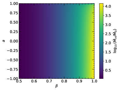
Figure 2: The accretion rate at the inner radius, $\dot{M}_{\text{in}}$, as a function of the black hole spin $a$ and temperature slope $\beta$, given in Equation (9).

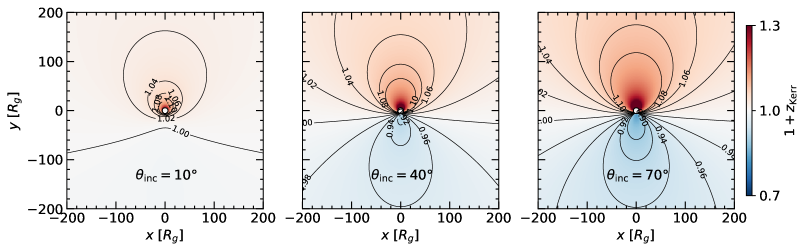
Figure 3: Example redshift map (Equation (13)) with Keplerian angular velocity (Equation (14)) for three different inclination angles ($10^{\circ}$, $40^{\circ}$, and $70^{\circ}$ from left to right). Here we fix the black hole spin to $a=0$.

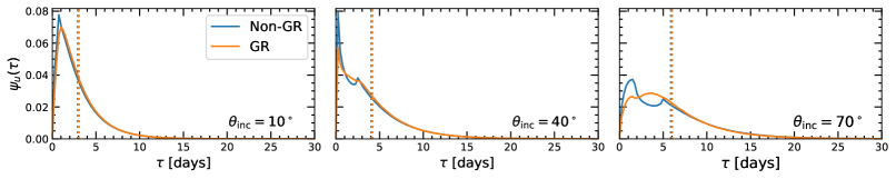
Figure 4: Example transfer function for the $u$-band without general relativistic (GR) effects (blue) compared to the case where we include GR effects (orange) for three different inclination angles ($10^{\circ}$, $40^{\circ}$, and $70^{\circ}$ from left to right). The mean time delays are given by the vertical dotted lines. We use the parameters: $\log_{10}(M/M_{\odot})=9$, $\beta=0.75$, $\lambda_{\text{Edd}}=0.1$, $a=0$, $H=16R_{g}$, $z=4$, $f_{\text{lamp}}=0.005$. Note that the GR effects include using the NT instead of the SS temperature profile and the gravitational redshifting and Doppler shifting due to the Kerr black hole.

We include general relativistic gravitational redshifting and Doppler shifting due to the Kerr black hole. In the rest frame of the disk, the effective temperature of each region of the disk is converted to disk flux through blackbody radiation:

$$B(\lambda_{e},T_{\text{eff}})=\frac{2hc^{2}}{\lambda_{e}^{5}}\left(\frac{1}{e^{hc/\lambda_{e}k_{\text{B}}T_{\text{eff}}}-1}\right)g^{4},$$ (11)

where $h$ is the Planck constant, $k_{B}$ is the Boltzmann constant, $\lambda_{e}$ is the emitted photon wavelength, and $g=1/(1+z_{\text{Kerr}})$ is the redshift factor due to both gravitational redshifting and relativistic Doppler beaming effects near the Kerr black hole (Cunningham & Bardeen, 1973). When simulating our transfer functions, we want to use the photons emitted at a redshift $\lambda_{e}$ that will correspond to the observed wavelengths $\lambda_{\text{obs}}$, in our case the effective wavelength of each LSST waveband. We must therefore account for the cosmic redshifting of the photon as well as the gravitational redshift and relativistic Doppler shifting from the Kerr black hole. An emitted photon will be observed at a wavelength:

$$\lambda_{e}=\frac{\lambda_{\text{obs}}}{(1+z_{\text{Kerr}})(1+z)},$$ (12)

where $z$ is the cosmic redshift. The redshifting due to the Kerr black hole geometry can be approximated by:

$$1+z_{\text{Kerr}}=\frac{(1+\Omega_{K})r\sin(\theta)\sin(\phi)}{\sqrt{-g_{tt}-2g_{t\phi}\Omega_{K}-\Omega_{K}^{2}g_{\phi\phi}}},$$ (13)

where each $g_{\mu\nu}$ are the metric components of a Kerr space-time, $\Omega_{K}$ is the angular velocity, $\theta=\theta_{\text{inc}}$ is the inclination angle of the disk, and $\phi$ is the azimuthal angle (Luminet, 1979; Bhattacharyya et al., 2001; Mastroserio et al., 2018; Heydari-Fard et al., 2023). We approximate this effect without the need for general relativistic ray tracing by ignoring the effects of light bending and assuming the accretion disk orbits the black hole at Keplerian angular velocity:

$$\Omega_{K}=\frac{c/R_{g}}{(R/R_{g})^{3/2}+a},$$ (14)

where the disk rotates in a circular orbit around the black hole (Abramowicz & Fragile, 2013; Mastroserio et al., 2018). In this way, we can efficiently implement general relativistic effects into our auto-differentiable accretion disk simulation. An example redshift map for different disk orientations is shown in Figure 3. The spin has very little effect on the redshift map except in the inner region of the disk near the ISCO. We find approximating the redshifting due to the Kerr black hole to be nearly identical to the full raytracing implementation of Sim5 (Bursa, 2017, 2018; Best et al., 2024b) for the general relativistic tracing around a Kerr black hole. In Figure 4, we show example transfer functions with and without all the general relativistic effects. At typical rest-frame wavelengths and low inclination, these effects have minimal impact on the transfer functions. However, at high redshifts and large inclination, where the shorter wavelengths allow us to probe the inner regions of the disk, these effects can alter the shape of the transfer function, although the mean time remains nearly unchanged. In this example we use a redshift of $z=4$, but the difference is noticeable at high inclination even at lower redshifts.

From the temperature profile defined in Equation (2.2), the blackbody flux in Equation (11), and standard time lags of the lamppost thin-disk model, we can generate the transfer functions (Cackett et al., 2007). See Chan et al. (2024) for a full derivation of the transfer function. In order to be computationally efficient and due to constraints with GPU memory, we want to minimize the number of pixels we need in the grid to accurately calculating the transfer functions. We define an effective radius of the accretion disk by numerically solving for $k_{B}T_{\text{eff}}(R_{c})=hc/\lambda$, where we use the wavelength of the reddest band. To account for cases where there is no solution, we define a characteristic radius by:

$$R_{c}=\operatorname*{argmin}_{R}\Big{(}\big{|}k_{B}T_{\text{eff}}(R)-hc/\lambda\big{|}\Big{)},$$ (15)

and calculate the transfer function using a $1000\times 1000$ grid out to $100R_{c}$. This effectively calculates the disk out to an infinite outer radius, since the flux decays to an insignificant amount well before $100R_{c}$. The characteristic radius is the same as in Chan et al. (2024) but using the full accretion disk model, so cannot be solved for analytically. The transfer functions introduce a wavelength dependent time lag:

$$\bar{\tau}_{\lambda}=\frac{\int_{0}^{\infty}\psi(\tau,\lambda)\tau d\tau}{\int_{0}^{\infty}\psi(\tau,\lambda)d\tau}.$$ (16)

We normalize the transfer functions to represent a probability distribution such that: $\int_{0}^{\infty}\psi(\tau,\lambda)d\tau=1$ for all $\lambda$. The transfer functions are calculated out to 800 days, enough so going out further is insignificant even for the largest mass black holes. We evaluate the transfer functions on daily intervals. The influence that each parameter has on the mean time delays and standard deviation of the transfer functions can be found in Appendix B.

2.3 Spectrum Model

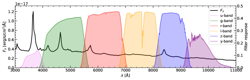
Figure 5: Example simulated quasar spectrum using the continuum of our accretion disk model and templates from Temple et al. (2021) to include the emission lines, host galaxy flux, extinction, the Lyman-alpha forest, and the Lyman-limit system. The filter responses of the six LSST bands are included from Kirkby et al. (2023). We can integrate the quasar spectrum across the filter responses to obtain the observed flux in each filter. The parameters of the example spectrum are: $\log_{10}(M/M_{\odot})=8$, $\beta=0.75$, $\theta_{\text{inc}}=45^{\circ}$, $\lambda_{\text{Edd}}=0.1$, $a=0$, $H=16R_{g}$, $z=2$, $f_{\text{lamp}}=0.005$, and $\text{E(B-V)}=0.1$.

In addition to the transfer functions, we model the quasar spectrum to obtain the mean flux in each broadband filter consistently with the accretion disk parameters. We do not need to model the spectrum in the auto-differentiable simulation (although we could), since the mean brightnesses of each waveband are a free parameter fit to the observations by the machine learning model, instead of being fixed by the accretion disk parameters.

To model the mean brightness in each band, we need to generate the quasar spectrum and then integrate it across the response function of each bandpass filter. Our accretion disk model that we defined in Section 2.2 can evaluate the mean flux of the disk at each wavelength for a given luminosity distance. We evaluate the mean fluxes corresponding to the observed wavelengths of the LSST filters (3,000–11,000Å) to generate the continuum spectrum. To properly model the quasar spectrum, however, we need to also include the emission lines, flux from the host galaxy, spectral reddening due to extinction from dust along the line of sight, contamination in the Lyman-alpha forest, and the Lyman-limit system. These effects have been previously modeled by Temple et al. (2021) and calibrated for redshifts $0<z<5$. We use the spectrum model of Temple et al. (2021), but replace the continuum from a broken power-law to the continuum generated from our accretion disk model. They use a set of templates to include the spectral bands, host galaxy flux, and extinction. The cutoff of the Lyman-limit system sets flux at a rest-frame wavelength of $\lambda<912\text{\AA}$ to zero. Once the full spectrum is obtained, we use speclite (Kirkby et al., 2023) to integrate the flux across the LSST broadband filters and obtain the mean magnitude of each waveband. Figure 5 shows an example simulated quasar spectrum with the LSST response functions. We note that the inclusion of the general relativistic effects can impact the mean brightness, since the black body flux is proportional to a factor of $(1+z_{\text{Kerr}})$ (See Equation (11)), although the impact of this is typically minor.

We first calculate the absolute magnitude of the $i$-band $M_{i}$ from the continuum, which is used to set the scaling of the emission lines and host galaxy. We add an additional scatter to our spectrum by a Gaussian random value with standard deviation of 0.1 mag to $M_{i}$ to account for mismatch between our simulation and the data. The other main parameter is the extinction strength E(B-V), which we randomly draw from a half Gaussian with mean 0 and standard deviation 0.075. The extinction has a significant effect on the quasar brightness. We further add additional scatter by varying the emission lines by controlling the relative scale height of the H-alpha, Lyman-alpha, and near line region, which we vary by a Gaussian with standard deviation 0.05. In real quasar data, individual emission lines can further vary in width and strength depending on the accession disk parameters and the broad line region of the disk. We include an additional scatter in the mean brightness of each band drawn from a Gaussian distribution with mean 0 and standard deviation 0.025 mag. We also include an additional constant offset to all bands also drawn from a Gaussian distribution with mean 0 and standard deviation 0.025 mag.

We limit the redshift to the range of $z\in[0.1,5.0]$, which includes the vast majority of quasars that will be observed by LSST. Within our selected redshift range, due to the Lyman-limit system, we do not always observe across all bands. The bluest band of LSST starts at $3000\text{\AA}$, so if the Lyman-limit system cutoff is redshifted past this range, parts of the LSST observations will be affected. At the highest redshifts, both the $u$ and $g$ bands will not be observed at all. To keep within the observational range of LSST, if the mean magnitude of the $i$-band is greater than 27 magnitude or less than 13 magnitude, then we resimulate a new quasar with a random set of parameters. This can happen when we have a low mass quasar at high redshift.

We obtain the mean brightness of each band both with and without the host galaxy, because the host galaxy flux should not be variable. The driving signal is produced in magnitude first with mean zero and standard deviation $\sigma$, and added to the mean magnitude of each band without the host galaxy contribution. We then convert from magnitude to flux and convolve with each transfer function kernel, and then add the flux from the host galaxy. Finally, we convert back from flux to magnitude.

We generate the driving signal eight times larger than needed to set the mean and standard deviation asymptotically to the longer signal. We then take the first eighth of the signal, where the local mean and standard deviation will not be the same as their asymptotic values. This is particularly important when $\nu_{b}^{-1}$ is a similar timescale to the length of the simulated light curve, so the $\sigma$ we predict represents the asymptotic variability strength of the driving signal. When constructing the training set, the driving signal is set to the normalization of the reference $i$-bands brightness before convolving with the transfer functions, since its mean brightness is arbitrary.

2.4 Parameter Ranges

The parameters to generate our light curves are given in Table 1. The light curves are simulated with 12 physical parameters, 4 for the driving variability and 8 for the accretion disk. The driving variability depends on its standard deviation $\sigma$, the break frequency $\nu_{b}$, and the low and high frequency power-law $\alpha_{L}$ and $\alpha_{H}$. The black hole geometry is determined by its mass $M$ and dimensionless black hole spin $a$. The quasar is at an inclination angle $\theta_{\text{inc}}$ (with $0^{\circ}$ being face on) and a redshift $z$. We also vary the corona height $H$, corona X-ray strength $f_{\text{lamp}}$, asymptotic viscus temperature slope $\beta$, and Eddington ratio $\lambda_{\text{Edd}}$. When sampling the light curves, we draw each parameter uniformly from its minimum and maximum range. There are also additional parameters related to the quasar spectrum that influences the mean magnitudes, in particular the extinction strength E(B-V). These however, are nuisance parameters for the purposes of this work and are not predicted by our network.

Table 1: Parameters and ranges to create a mock light curve, and predicted by our machine learning model. The parameters are sampled uniformly between the minimum and maximum given in the table. The top four parameters are for the X-ray driving variability, while the bottom eight parameters relate to the black hole and accretion disk reprocessing. We also have additional parameters related to determining the mean magnitude of each band not predicted by the network, in particular the extinction strength E(B-V).

Parameter	Description	Min.	Max.
$\sigma/\text{mag}$	variability amplitude	0	0.5
$\log_{10}(\nu_{b}/\text{day}^{-1})$	break frequency	$-3.5$	0.0
$\alpha_{L}$	lower power-law	0.25	1.5
$\alpha_{H}-\alpha_{L}$	higher power-law	0.75	2.75
$\log_{10}(M/M_{\odot})$	black hole mass	7	10
$a$	dimensionless spin	$-1$	1
$\theta_{\rm inc}$	inclination angle	$0^{\circ}$	$70^{\circ}$
$(H-R_{\text{in}})/R_{g}$	corona height	0	50
$f_{\text{lamp}}$	lamppost strength	0.002	0.007
$\beta$	temperature slope	0.3	1.0
$z$	redshift	0.1	5
$\log_{10}(\lambda_{\text{Edd}})$	Eddington ratio	$-2$	0

We parameterize the ISCO height as $(H-R_{\text{in}})/R_{g}$, since the corona must always be above the ISCO. We parameterize $\alpha_{H}-\alpha_{L}$ instead of using $\alpha_{H}$ directly, because we expect $\alpha_{H}\geq\alpha_{L}$. The X-ray radiative efficiency factor $\eta_{X}=\eta/\lambda_{\text{Edd}}L_{X}/L_{\text{Edd}}$ where $L_{X}/L_{\text{Edd}}\sim 0.005$ (Ursini et al., 2020). We parameterize the lamppost strength which we define as $f_{\text{lamp}}=(1-A)L_{X}/L_{\text{Edd}}$ since the albedo and X-ray luminosity ratio are degenerate. The albedo ranges from $A=0$ for full absorption to $A=1$ full reflection, with typical value $A\sim 0.1$–$0.2$ (Ursini et al., 2020). The driving variability parameters are chosen to be consistent with measurements from Summons (2007). We evaluate the transfer functions at the effective wavelengths of each of the LSST bands (Huber et al., 2021).

2.5 Mock LSST Observations

After the UV/optical light curves are simulated, we degrade them to mimic LSST-like observing cadences and noise in the same way as Fagin et al. (2024b). The errors at each LSST observations are:

$$\sigma_{\text{LSST}}^{2}=\sigma_{\text{sys}}^{2}+\sigma_{\text{rand}}^{2},$$ (17)

where $\sigma_{\text{sys}}$ is the systematic error and $\sigma_{\text{rand}}$ is the photometric noise. The systematic error is set to $0.005$ mag, since this is the maximum value expected for LSST (Ivezić et al., 2019; Suberlak et al., 2021). The photometric noise depends on the brightness of each observation and is expected to follow:

$$\sigma_{\text{rand}}^{2}=(0.04-\gamma)x+\gamma x^{2}\quad(\text{mag}^{2}),$$ (18)

$$x=10^{0.4(m-m_{5})}$$

where $\gamma$ is a band-dependent factor, $m$ is the magnitude of each observation, and $m_{5}$ is the $5\sigma$ depth of a point source observed at the zenith the observation. We expect $\gamma_{u}=0.38$ and $\gamma_{g,r,i,z,y}=0.39$ (Ivezić et al., 2019; Sheng et al., 2022). We simulate LSST-like observations using rubin_sim with the baseline_v2.1_10yrs rolling cadence, which gives the time and $m_{5}$ of each observation. We produce a random sample of 100,000 LSST-like 10-year observations by sampling anywhere in the sky with 750–1000 total observations across all bands. This filters the light curve sample to include only the Wide Fast Deep observations, the main LSST survey (see Figure 1 of Prša et al., 2023).

At each observation, we randomly sample the error from a Gaussian with mean zero and variance $\sigma_{\text{LSST}}^{2}$. We combine the observations to the nearest one-day interval, averaging across $\sigma_{\text{rand}}^{2}$ if there are multiple observations in a band in the same interval. We simulate 10.5-year light curves with 10 years of LSST observations so our model is trained to reconstruct some time before and after the survey. The start time of the first LSST observation is randomly selected within the extra half-year of time. Any observation outside the range of 13–27 mag is not observed, which should be similar to the magnitude limits of LSST. To avoid confusing the network, we only include observations in a band that has at least 15 observations throughout the 10-years.

3 Machine learning model

3.1 Overview

The overall goal of our machine learning model is to solve the inverse problem in Equation (1) related to reconstructed the driving variability $X(t)$ and transfer function kernels $\psi(\tau|\lambda)$ given a set of noisy and sparsely sampled observations. Since the reprocessing is formulated as a convolution of the driving variability and transfer function, we are essentially training a neural network to solve a blind deconvolution problem. In general, recovering the transfer function kernels is an intractable problem because there is a degeneracy between the driving variability and kernels. We could instead treat the bluest band as an effective driving signal and define effective kernels with respect to it. This is what is done with JAVELIN, but then we sacrifice most of the physics of the reprocessing on the disk. To make the problem tractable, we parameterize the transfer functions through our auto-differentiable simulation $\psi(\tau|\lambda,\boldsymbol{\eta})$ where $\boldsymbol{\eta}$ is the vector of accretion disk parameters and given in Table 1. The driving signal is reconstructed using a latent SDE (Li et al., 2020; Fagin et al., 2024b), parameterized by the context at each time and the latent vector $\boldsymbol{z}$. We then solve for the flux by embedding the physics of the reprocessing of the driving variability into our neural network architecture by:

$$\underbrace{F_{\lambda}(t,\lambda|\boldsymbol{z},\boldsymbol{\eta})}_{\begin{subarray}{c}{\rm flux}\\ {\rm predicted}\end{subarray}}\propto\int_{0}^{\infty}\underbrace{X(t-\tau|\boldsymbol{z})}_{\begin{subarray}{c}{\rm latent}\\ {\rm SDE}\end{subarray}}\underbrace{\psi(\tau|\lambda,\boldsymbol{\eta})}_{\begin{subarray}{c}{\rm auto{\rm-}diff}\\ {\rm transfer\;function}\end{subarray}}\text{d}\tau,$$ (19)

where this convolution of the driving variability and transfer functions is evaluated numerically within our neural network. Our network also quantifies the uncertainty in the reconstructed $F_{\lambda}(t,\lambda$), $X(t)$, $\boldsymbol{\eta}$, the variability parameters, and the mean time delays $\bar{\tau}_{\lambda}$ coming from each reconstructed kernel $\psi(\tau|\lambda)$.

The input to the network is the brightness and error values (both in magnitude), for a total of 12 features at each time step (6 bands and 6 errors). For training stability, each band is normalized to have mean zero and standard deviation one, but the mean and standard deviation are used to predict the latent space of the SDE and the parameter posteriors. The reconstructed driving signal and UV/optical variability are unnormalized after they are generated by the network. For each band that is not observed at a given time step, we set both the brightness and error to a dummy value of zero to be masked by the network. The outputs of our network are: the best fit reconstruction of the UV/optical light curves, the reconstructed driving signal, predicted accretion disk and driving variability parameters and uncertainty, and the predicted relative time delays between each band and the $i$-band (arbitrarily chosen as the reference band) with uncertainties.

3.2 Proof of Concept Recurrent Inference Machine

We use a recurrent inference machine (RIM) to compare the reconstruction of our light curve with the observations, and iteratively adjust the accretion disk parameters by $\boldsymbol{\eta}_{i+1}=\boldsymbol{\eta}_{i}+\Delta\boldsymbol{\eta}_{i}$ and the latent space of the latent SDE by $\boldsymbol{z}_{i}=\boldsymbol{z}_{i}+\Delta\boldsymbol{z}_{i}$ in Equation (19) with iteration $i$ and initial values of zero. Due to constrains in GPU memory, this process can be computationally costly as only a small batch size can be used. We therefore train the network first without this process and then test training using the RIM with 3 iterations, although ideally we would use more iterations and train longer.

3.3 Model Architecture

The network has two main components: the context network of the latent SDE and a RIM network used only to adjust $\boldsymbol{\eta}$ and $\boldsymbol{z}$. Both contain bidirectional recurrent neural networks (RNNs) and begin with a GRU-D layer (Che et al., 2016), a type of Gated Recurrent Unit (Chung et al., 2014) layer that is designed to handle the masking and irregular sampling. The initial GRU-D layer is followed by two GRU layers (Chung et al., 2014). Each layer is made bidirectional by splitting each RNN layer into two, one that processes the time series forward and another backwards. The output of the RNN that processes the time series backwards is then flipped across its time axis and concatenated to the output of the forward RNN. We also use a transformer encoder after the RNN layers that is concatenated with the output (Vaswani et al., 2023). The output of the RNNs and transformers are followed by two fully connected layers.

The input of the context network is the observed light curve, padded for an additional 800 days to account for the extra time needed for the driving signal due to the length of the transfer function kernels. For the RIM network, we start with a predicted light curve at the mean of each band. The input to the RIM network is the predicted light curve $\hat{y}$, the observations $y$ with variance $\sigma^{2}$, the gradient of the observations $-2\bar{\sigma}^{2}\cdot m\cdot(y-\hat{y})/\sigma^{2}$, the z-score $\bar{\sigma}\cdot m\cdot(y-\hat{y})/\sigma$, and log-likelihood $\bar{\sigma}\cdot m\cdot(y-\hat{y})^{2}/2\sigma^{2}$, where $m$ masks all the unobserved points and the $\bar{\sigma}$ is the root mean variance of the observational noise which is included for stability so each input has units of magnitude. For the context network, we use the entire time vector for the latent SDE. We also have a two layer fully connected layer to get one value from the time dimension of the context and RIM networks by taking as input the first and last times and the mean and standard deviation across the time dimension. The output of the RIM network goes into a small network that is one GRU cell and a fully connected layer, with the hidden state of the GRU cell being updated with each iteration of the RIM. The context is also used to predict the parameters, latent space of the SDE, and normalization of the light curve.

There is an additional RNN without the transformer to produce uncertainty in the reconstructed driving and UV/optical variability with the same architecture but no transformer. We use one more RNN to project the output of the latent SDE to the mean and standard deviation on the observation space (see Fagin et al., 2024b). This RNN has a linear skip connect between the output of the SDE and a two layer bidirectional GRU based RNN.

There are multi-layer perceptrons (MLPs) to produce the posterior parameters of the accretion disk and variability, the latent space of the SDE, the normalization of the light curve, and the uncertainty in the time delay estimates. While $\boldsymbol{\eta}$ and $\boldsymbol{z}$ are adjusted iteratively, the rest are produced directly each iteration. Each MLP takes as input the context, the mean and standard deviation of the input light curve, as well as the other previous predicted parameters of the network, while $\boldsymbol{\eta}$ and $\boldsymbol{z}$ also uses the output of the RIM network. To adjust $\boldsymbol{\eta}$ and $\boldsymbol{z}$, we use an additional two-layer network, depending on the RIM network output and iteration number, that scales the updates by a factor dependent on the iteration count, allowing the network to gradually suppress changes as the RIM approaches convergence. There are also two MLPs in the latent SDE: the posterior drift function that decodes the context and latent vector, and the diffusion network that is applied element wise to satisfy the diagonal noise (Li et al., 2020). The latent SDE consists of an Itô SDE solver using the Euler–Maruyama numerical approximation scheme with time increments $\Delta t=0.0005$ over the time interval $[0,1]$. We use a Gaussian mixture model to parameterize the posterior of the accretion disk and variability parameters with 5 multivariate Gaussians (discussed further in Section 3.4). For the mixture coefficients, we use a softmax activation function to normalize them to probabilities. The variability parameters take as additional input the results from analyzing the driving signal by conducting multiple linear fits to different pieces of the power spectrum. We also use the mean, standard deviation, mean absolute deviation, total variation, and total square variation as well as the results of the two latent SDE MLPs at $z_{0}$. To obtain a vector of accretion disk parameters $\boldsymbol{\eta}$ from the posterior distribution, we sample from the Gaussian mixture model and take its mean. We use the mean times in the different reconstructed transfer functions to find the relative time delays with respect to the reference $i$-band, and we assign uncertainties to the prediction. To normalize the light curve, we include 3 terms, a mean and standard deviation for each bands brightness in magnitude, and an additional bias term in the flux. The additional bias term in the flux is required since the host galaxy can contribute non-variable flux. We note that when a band is not observed (such as the $u$ and $g$ bands at high redshift), its brightness is set to the maximum limit of $27$ mag and standard deviation set to $1$ mag.

Each MLP consists of four fully connected layers. The RNNs uses tanh activation, transformers use GELU (Hendrycks & Gimpel, 2023), and fully connected layers uses LeakyReLU (Maas et al., 2013). Whenever appropriate, we include residual skip connections (He et al., 2015) and layer norm (Ba et al., 2016). We use a hidden size of 256, transformer encoder size of 512, context size of 128, and latent size of 16. The transformer encoder has 5 layers, 8 heads, and uses a sinusoidal time embedding. Our model is built in PyTorch (Paszke et al., 2019) and has 38,551,054 parameters. Around 85% of the parameters are part of the two transformers in the model.

3.4 Uncertainty Qualification and Loss

The driving variability is modeled as a latent SDE. Unlike in Fagin et al. (2024b), we do not sample the latent space of the SDE from a posterior distribution, but instead just predict $z_{0}$ directly. We find this to significantly improve the performance of the light curve reconstruction, since otherwise the reconstructed driving signal is not as adaptable. Our light curve reconstruction is found by convolving the driving variability with the predicted transfer function kernels and scaling it to best match the observed data. We include into the loss the negative Gaussian log-likelihood between the reconstructed and true light curve including the unobserved driving signal and averaged across the bands:

$$-\log(\mathcal{L})=\frac{1}{N}\sum_{t=1}^{N}\frac{(y_{t}-\hat{y}_{t})^{2}}{2\hat{\sigma}_{t}^{2}}+\frac{1}{2}\log(2\pi\hat{\sigma}_{t}^{2}),$$ (20)

where $y$ is the true light curve, $\hat{y}$ is the predicted mean, $\hat{\sigma}^{2}$ is the predicted variance, and $N$ is the number of time steps. We predict $\log(\hat{\sigma}^{2})$ instead of $\hat{\sigma}$ for stability and to force the variance to be positive. As mentioned in Section 2.3, not all bands are observed due to the brightness limits of LSST and the Lyman-limit system. There is an additional mask in Equation (20) such that we only attempt to reconstruct bands that contain observations, although we always reconstruct the unobserved driving signal. We include an additional term into the loss to ensure that our mean prediction closely matches the context points at each observation:

$$-\log(\mathcal{L})=\frac{1}{N_{\text{obs}}}\sum_{t=1}^{N}m_{t}\cdot\frac{(y_{t}-\hat{y}_{t})^{2}}{2\sigma_{\text{LSST},t}^{2}},$$ (21)

where $\sigma_{\text{LSST}}$ is the photometric and systematic error of each observation, $m_{t}$ is a mask that is 1 if a band is observed at a time step $t$ and 0 if it is not and $N_{\text{obs}}=\sum_{t=1}^{N}m_{t}$ is the number of observations. The additional term in the negative log-likelihood $\frac{1}{2}\log(2\pi\sigma_{\text{LSST},t}^{2})$ does not depend on our predictions so is not included.

For the parameter inference, we use a multivariate Gaussian mixture model. Each multivariate Gaussian is has negative Gaussian log-likelihood:

$$-\log(\mathcal{L})=\frac{1}{2}(\boldsymbol{y}-\boldsymbol{\hat{y}})^{\top}\Sigma^{-1}(\boldsymbol{y}-\boldsymbol{\hat{y}})+\frac{1}{2}\log(2\pi|\Sigma|),$$ (22)

where each $\boldsymbol{y}$ is the vector of true values of our parameters, $\boldsymbol{\hat{y}}$ is the vector of our predicted means, and $\Sigma$ is the covariance matrix of the prediction. To ensure that the covariance matrix is symmetric, positive semi-definite, and non-singular, we predict the lower triangular matrix $L$ representing the Cholesky decomposition of the covariance matrix $\Sigma=LL^{\top}$. The diagonal of $L$ must be positive, so we take the softplus of each element of its diagonal. An $m\times m$ lower triangular matrix will have $m(m-1)/2$ free parameters, in our case $m=12$. We minimize in the loss function the total negative log-likelihood of the Gaussian mixture model:

$$-\log(\mathcal{L})=-\log\left(\sum_{i=1}^{n}a_{i}\mathcal{L}_{i}\right)$$ (23)

where each $a_{i}$ are the Gaussian mixture coefficients of our $n=5$ multivariate Gaussians and $\sum_{i=1}^{n}a_{i}=1$.

We additionally predict the time delays of each band with respect to the reference $i$-band. These time delays are based on our predicted transfer functions, but we also predict the lower triangular matrix to assign multidimensional uncertainty using Equation (22). We include measuring the time delays in the loss function, even for bands that are unobserved. The loss function is the sum of the four components: the light curve reconstruction, the fit to the observations, the parameter predictions, and time delay predictions. We weighted the loss as $2,1,1,1$ respectively, since we are most interested in the parameter predictions. When using RIM, we scale the loss proportional to the iteration number to weight the later iterations more, since we only use the results of the final iteration.

We use uniform priors for the variability and accretion disk parameters when simulating our light curves, given in Table 1. When training our network, we reparameterize the parameter labels from their physical values to between zero and one and then take the logit to scale them from $-\infty$ to $\infty$. We then evaluate the negative log-likelihood of our parameter posterior in this logit space. We take the sigmoid after drawing samples from the posterior, scaling the predictions back to between zero and one, before scaling back to the original physical range. This transformation prevents any posterior probability from being wasted in physically impossible parameter space or outside the range of the training set (for example, we want to restricting the spin to $-1<a<1$).

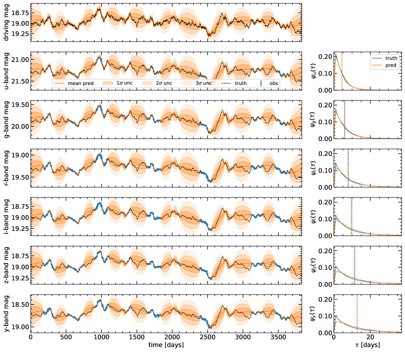
Figure 6: The left panels show an example reconstruction (orange) of a simulated 10.5-year UV/optical quasar light curve (black) from our nominal test set with LSST-like observations (blue). The mean prediction is given by the orange solid line, with 1$\sigma$, 2$\sigma$, and 3$\sigma$ uncertainties highlighted. The UV/optical bands are reprocessed from the reconstructed driving signal (top panel) using the predicted transfer functions (right panels), with the mean time delays indicated by the dashed vertical lines.

3.5 Training

We train our network with 100,000 light curves per epoch that are randomly regenerated on the fly. Regenerating the training set each epoch prevents overfitting by training with many more unique examples. This is especially important since our model has a large number of free parameters. We use fixed test sets of 10,000 light curves to evaluate the performance of our model after training.

Our network is trained for 30 epochs using the Adam optimizer (Kingma & Ba, 2017). We train our network with 4 A100 GPUs (80 Gb) in multiple stages. We first train our network with only 1 iteration to train faster. We use an initial learning rate of $8\cdot 10^{-4}$ that is exponentially decayed by 0.95 each epoch, and a batch size of 26 per GPU (the maximum that fit in GPU memory). In the final 4 epochs, we use 3 iterations with a batch size of 14 to test the RIM technique. Throughout training, we use gradient clipping with a maximum gradient norm of 250 to help prevent exploding gradients. Training took around 3 weeks.

4 Results

4.1 Light Curve Reconstruction Performance

An example reconstructed UV/optical light curve, X-ray driving signal, and transfer function from the nominal test set is shown in Figure 6. Our network is able to properly quantify the uncertainty in its reconstruction, and reconstructs the driving signal and transfer functions using just the UV/optical observations.

Table 2: Light curve reconstruction performance of our latent SDE model compared to the GPR baseline in terms of the negative Gaussian log-likelihood given in Equation (20). We test the pretrained model using the nominal broken power-law (BPL) driving signal, and out-of-distribution driving signals including a DRW, BPL+Sine, Sine, sawtooth, and square wave. The values reported are the median $\pm$ median absolute deviation on the median across our test sets of 10,000 light curves. Lower is better and is shown in bold.

Driving Signal	Latent SDE	GPR
BPL	$\boldsymbol{-1.528\pm 0.007}$	$-1.409\pm 0.007$
DRW	$\boldsymbol{-1.214\pm 0.007}$	$-1.129\pm 0.007$
BPL+Sine	$\boldsymbol{-1.276\pm 0.007}$	$-1.111\pm 0.007$
Sine	$\boldsymbol{-1.847\pm 0.009}$	$-1.765\pm 0.012$
Sawtooth	$\boldsymbol{-1.221\pm 0.007}$	$-0.971\pm 0.008$
Square Wave	$\boldsymbol{-1.098\pm 0.007}$	$-0.933\pm 0.007$

To evaluate the performance of our network, we compare it to a multitask GPR baseline on our test sets. The GPR baseline is described in Appendix C in addition to an example reconstruction of a UV/optical light curve. To test the robustness of our network to irregular variability, we use additional test sets with different out-of-distribution driving signals. The median negative Gaussian-log likelihood across each test sets is given in Table 2. We find that our machine learning model outperforms the GPR baseline for each driving signal, despite being trained only using the bended broken power-law. The exact parameter space of each driving signal is given in Appendix D. To demonstrate the performance differences between our latent SDE model and the GPR baseline are statistically significant, we conduct a paired $t$-test and find extremely low $p$-values (less than $10^{-6}$). We choose to test our model on driving signals that are variable (BPL, DRW), quasi-periodic (BPL+Sine), and periodic (Sine, sawtooth, square wave). In each case, we are still able to predict the accretion disk parameters despite using out-of-distribution driving signals. We demonstrate this in in Appendix D for the case of the black hole mass, but in all cases, we are able to predict the redshift, temperature slope, and Eddington ratio similar to the case for the bended broken power-law. We also show an example light curve reconstruction using a sawtooth driving signal to demonstrate how our model fits an out-of-distribution light curve.

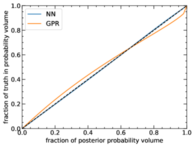
Figure 7: The fraction of the truth encompassed within the posterior probability volume across the nominal test set for the UV/optical light curve reconstruction using for our neural network (NN) compared to the GPR baseline. Perfect uncertainty calibration is shown by the black dashed line along the diagonal.

In Figure 7, we show that the uncertainties we predict in our UV/optical light curve reconstruction is well calibrated, while the GPR baseline is misaligned. We may expect the GPR baseline to be misaligned, since it assumes a DRW kernel, while our driving signal is generated from a more general broken power-law PSD and convolved with the transfer function kernels for each band.

4.2 Parameter Inference Performance

An example predicted parameter posterior from our nominal test set is given in Appendix E. In Figure 9, we show the median prediction compared to the true value for each parameter across the test set, demonstrating the ability of our model to predict each parameter. In this figure, we only show the median but a full posterior is predicted for each light curve. We show a similar figure using the median with $1\sigma$ confidence interval for 100 example light curves in Appendix E. In Figure 8, we show that the uncertainties we predict in our parameter posteriors are relatively well calibrated.

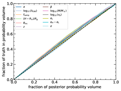
Figure 8: The fraction of the truth encompassed within the posterior probability volume across the nominal test set for each of the predicted parameters. Perfect uncertainty calibration is shown by the black dashed line along the diagonal

Figure 9: Median prediction compared to the true value for each predicted parameter (given in Table 1) across the nominal test set. The ideal case where the median prediction matches the truth is given by the black dashed line across the diagonal.

For the accretion disk parameters, we are able to predict the mass, temperature slope, Eddington ratio, and redshift. The network struggles to predict the inclination angle and black hole spin but can make some constraints, while the corona height and lamppost strength cannot be predicted at all. We show the influence that each parameter has on the transfer functions in Appendix B, which explains why some of the accretion disk and black hole parameters can be predicted more easily than others, although there is additional information in the mean brightnesses. The mass and temperature slope predictions are better than in Fagin et al. (2024b) due to modeling the mean brightness of each band. We can predict the Eddington ratio and redshift while Fagin et al. (2024b) could not at all. Our network cannot predict the inclination angle well, however, since we are now properly modeling the mean brightness of each band and include host galaxy contribution, so the brightness suppression from the transfer functions is not as informative. The shape of the predicted redshift is not continuous due to the $u$ and $g$ bands being suppressed at high redshift. In addition, we are able to predict the bended broken power-law PSD parameters of the driving signal, although it is more challenging than the DRW parameters (see Fagin et al., 2024b). This is due to the bended broken power-law having two additional parameters corresponding to the low and high frequency limits of the power spectrum. These parameters are approximately degenerate, for example in Figure 1, the driving variability in the topmost panel is very similar to that of the bottom panel despite changing each parameter. As discussed in Section 4.1, we demonstrate in Appendix D that our model can still infer the black hole mass with out-of-distribution driving signals, and the performance of all accretion disk parameters remains consistent with the results shown in Figure 9.

4.3 Example Relative Rime Delay Inference

Figure 10: Example predicted posterior distribution for the time delay measurements using a reference $i$-band for the same test light curve shown in Figure 6. The mean predictions come from the reconstructed transfer functions, while the uncertainties are separately quantified by our network. The diagonal elements display marginal distributions with the median and 1$\sigma$ levels indicated by dashed lines. The central elements depict 1$\sigma$, 2$\sigma$, and 3$\sigma$ contour levels. The true time delays are overlaid in blue.

The mean time delays between bands are found directly from the mean times of our predicted transfer functions so that our model is entirely self-consistent. The time delay differences are defined with respect to the $i$-band as a reference. Our model predicts time delays even in the case where we do not observe the bluest bands, since we still have the transfer functions corresponding to our predicted accretion disk parameters. Our network then produces uncertainties associated with the mean time delays by predicting the lower triangular matrix $L$ of its covariance matrix $\Sigma=LL^{\top}$. An example posterior of the time delays measurements is shown in Figure 10. The time delay posterior is directly inferred by our network instead of requiring MCMC sampling.

4.4 Recurrent Inference Machine Evaluation

Figure 11: Loss compared to each iteration of the RIM procedure, averaged across the nominal test set.

We evaluate the performance of our model using a RIM for three iterations. The loss compared to the iteration number is shown in Figure 11. The RIM procedure does show a minor improvement in the performance of the model compared to using just a single iteration.

5 Discussion

We constructed the first machine learning approach to model the driving variability, accretion disk reprocessing transfer functions, and time delays in a single unified framework by embedding the accretion disk reprocessing model into our neural network architecture. This makes our predictions more interoperable compared to modeling each process individually. Our method enables the fast inference of accretion disk and variability parameters, time delays between wavebands, and the reconstruction of the driving signal and UV/optical bands.

Unlike traditional methods of measuring time delays, our model can use information related to the mean brightness and variability to inform our network on the accretion disk parameters and time delay measurements. We also model the driving variability in a free-form way (i.e. using a latent SDE) instead of using a DRW process like JAVELIN or a Fourier series like CREAM. In addition, we directly predict the variability parameters of the driving signal without requiring it to be Gaussian process. Furthermore, we can predict more parameters of the accretion disk including the mass, Eddington ratio, redshift, and temperature slope and the variability parameters of the unobserved driving signal. Comparatively, CREAM typically only measures the $M\dot{M}$. While our new method is more computationally demanding to train than Fagin et al. (2024b) due to having many more parameters and the use of RIM, during inference it is still quick enough to easily apply to the tens of millions of quasar light curves expected from LSST in several hours. Specifically, the average inference time on our GPUs using a batch size of 64 is about 27 minutes per million light curves using 3 iterations of the RIM, or 7 minutes using 1 iteration. Comparatively, using JAVELIN or CREAM on tens of millions of light curves would be infeasible.

LSST will observe tens of millions of quasars, and only a small fraction of them will get follow-up spectra to obtain precise redshift measurements. Therefore, most quasars will rely on photometric redshifts. In theory, the photometric redshift predictions of our network can outperform simple photometric redshift estimators based on the brightness differences between broadbands. This is because the photometric redshifts should depend most strongly on the asymptotic brightnesses of each band, and our model incorporates modeling the time variable brightness. Furthermore, the redshift also effects the time delays and driving variability time scale, so by analyzing all these processes in a unified framework, we can outperform methods relying on static data. Quasars that do have follow-up spectra can be better constrained by using the redshift as a prior in our network. The mass and other properties of the accretion disk may be constrained from measurements of the broad-line region (Panda et al., 2019), which could also be used to inform our network.

We are the first to build an auto-differentiable simulation of quasar transfer functions, allowing us to jointly model quasar variability and accretion disk parameters in a physically motivated way within our neural network. Although our auto-differentiable simulation utilizes a specific accretion disk model, it can be substituted with any auto-differentiable simulation that can be parameterized by a set of physical parameters or latent space. In theory, more complicated models of quasar variability involving hydrodynamic simulations and raytracing could be developed in an auto-differentiable simulation, although the prospects of this are likely computationally infeasible. A more reasonable approach could be to train a neural network to approximate transfer functions from complex simulations and embed the fixed, pretrained model into the neural network architecture. Instead of being model dependent, we could also use analytic functions such as using simple top hat transfer functions like JAVELIN or a set of Gaussians defined with respect to the bluest band (i.e. only five transfer functions for six bands since the bluest band is treated as the effective driving variability). One may also reconstruct the effective transfer functions in a free-form way, but this would require using regularization or through a complete set of basis functions to make the inverse problem tractable. In these cases, the X-ray driving variability would not be reconstructed, and we defer testing and developing these methods for future work. This may be particularly useful for measuring cosmological time delays between different images of gravitationally lensed quasars (Wong et al., 2019).

Our network is ready to be applied to the entire LSST sample. We assume that the light curves used in training, however, are type 1 quasars. It is important that we filter out the type 2 quasars from the LSST sample before applying our network. This could be done using another neural network which classified quasar light curves between type 1 and type 2. Typically type 2 quasars can be distinguished since they have very lower levels of variability, so we may simply filter out light curves with variability less than some threshold.

In this work we did not account for time delays that may arise from the broad line or near line regions of quasars. Modeling the BLR is difficult since its geometry is not well known. Including the BLR into our simulation would introduce a large number of additional parameters (Best et al., 2024b). The time delays caused by the BLR can cause our method to overestimate the recovered black hole mass, since the BLR can introduce larger time lags. However, this is also the case for traditional sampling methods like JAVELIN and CREAM. There may also be other areas in which our accretion disk model does not account for such as a radially dependent albedo or color correction factors to the blackbody radiation. Furthermore, the thin-disk NT model may break down at high Eddington ration, and different disk models such as the slim-disk (Abramowicz et al., 1988) may be more accurate. These changes in disk model may already be partially accounted for by the inclusion of the accretion rate wind model (Equation (8)). There may also be long negative time lags at the viscous timescale of the disk (Yao et al., 2023; Secunda et al., 2024), which our model could be adapted to predict to learn about the vertical structure of the disk. In this work, we test that our model is robust to different out-of-distribution driving signals, but it would be useful to test how our pretrained model behaves for different disk models.

Once LSST data becomes available, we can fine-tune our model with the exact cadences of LSST and can train using self-supervised on the LSST observations. This would help generalize the machine learning model to the data, so our light curve reconstruction better fits the observations. The light curve reconstruction and parameter inference are linked through our auto-differentiable simulation of the accretion disk, so by fine-tuning the model on the observations, we can potentially improve all aspects of our predictions. In addition, the parameters of the broken power-law driving signal may be related to properties of accretion disk and black hole (Arevalo et al., 2023). In our training set, we choose to keep them independent so that these correlations could potentially be measured by our model without bias. However, our model could improve its predictions by finding these correlations when fine-tuning with the real data. Furthermore, we train our model on the nominal Wide Fast Deep survey. A subset of quasars will be monitored in the Deep Drilling Fields, and our network can take advantage of the increased sampling rate. Fine-tuning our model with context from the Deep Drilling Field quasar sample may be particularly beneficial.

We find the parameters of the broken power-law to be more difficult to predict than the DRW parameters used in Fagin et al. (2024b). This is because there are two additional parameters of the driving variability model, and the additional degrees of freedom introduces degeneracies. Here we parameterized the driving variability as a bended broken power-law, since it has been found to fit X-ray variability data. Some authors such as Papoutsis et al. (2024) fix the lower frequency slope to $\alpha_{L}=1$, which would get rid of degeneracies, and our predictions for $\nu_{b}$ and $\alpha_{H}$ would significantly improve. We choose to keep the bended broken power-law more general to account for the wide range of variability possible in LSST. We could, however, use any parameterization of the PSD to train our model. Furthermore, we compared the performance of our model to a GPR baseline that uses a DRW kernel. Higher order CARMA processes may show some improvements compared to the DRW kernel (Yu et al., 2022). However, all Gaussian processes require selecting a kernel and will not be able to use the information related to the mean brightness of each waveband. One possibility is to use neural inference Gaussian processes (Danilov et al., 2022) that could potentially utilize features learned across a training set. Our light curve reconstruction may be benchmarked compared to neural inference Gaussian processes in future work, or they could be included as a component of our network.

As far as we are aware, this work represents the first application of transformers to model quasar variability. To process the irregularly sampled time series, we first use GRU-D and GRU layers and then transformer encoders concatenated with the output. The GRU-D can handle the irregular sampling in a more motivated way than the transformers, and we find using the transformers alone struggles to converge. Combining both RNN and transformer architectures yielded good convergence while still allowing us to expand our model to tens of millions of parameters, by far the largest deep learning model applied to quasar variability to date. In future work, we may also test other types of networks. For example, Schirmer et al. (2022) introduced the continuous recurrent unit, which is a probabilistic recurrent architecture that includes a hidden state that evolves as a linear SDE. This may also be combined with transformers, similar to how we combined RNNs and transformers in our model. In addition, we considered implementing mixed precision in our network to save GPU memory and reduce training time. However, we found that using lower precision led to numerical issues in the gradients, so it was not to include at this time but may used in the future. We also bin the time series and transfer functions to daily time intervals in this work. Ideally we would use smaller bins, but we are limited by GPU memory and training time. Using daily intervals could negatively impact the parameter inference of quasars with smaller mass black holes, where the time delays can be of order of one day.

We use our framework to iteratively improve the light curve reconstruction and accretion disk parameter estimation with a RIM by analyzing the residuals between the predicted light curve and observations. We found the RIM to have only a minor advantage compared to using a single iteration. This is likely due to several factors. For example, we pre-trained our model using a single iteration to save on training time. Furthermore, we use a very large model with tens of millions of parameters, and it may be the case that a minima is achieved with a single iterations. Furthermore, our model is stochastic, irregularly sampled, and noisy. Therefore, we cannot reconstruct the time series to the pixel level, as is the case for image reconstruction tasks where RIM has traditionally been applied. The RIM technique may be more advantageous for well sampled light curves, such as in the Deep Drilling Fields.

The framework developed in this work offers significant potential for anomaly detection in various contexts. For instance, the latent space of the SDE can be used in an unsupervised way to identify out-of-distribution sources of variability by comparing it to the typical distribution of quasar light curves or employing methods like Isolation Forests. Additionally, by analyzing the reconstructed driving signal, we may detect quasi-periodic signals that could indicate the presence of a supermassive black hole binary. The model could also be extended through supervised learning to classify light curves as belonging to phenomena such as supermassive black hole binaries, changing-look AGN, flaring events, tidal disruption events, or gravitational microlensing. This would involve either incorporating these effects into the training set or fine-tuning the model using real data.

Some of the accretion disk parameter are difficult to predict for individual quasars. Hierarchical inference could be used with the entire LSST sample to estimate the population-level distributions of the parameter space (Wagner-Carena et al., 2021). For example, the population-level distribution of the temperature slope $\beta$ could be used to test accretion disk and wind models, despite being challenging to constrain for individual quasars with only six bands. Furthermore, we could measure the relationship between driving variability parameters $\nu_{b}$, $\sigma$, $\alpha_{L}$, and $\alpha_{H}$ and black hole properties like the mass.

6 Conclusions

Our machine learning model and auto-differentiable accretion disk simulation are open sourced and available at: https://github.com/JFagin/Quasar_ML. Our model fits the UV/optical variability, reconstructs the driving variability signal, predicts accretion disk and variability parameters, and measures the relative time delay between bands, all self-consistently using a neural network that incorporates the physics of the accretion disk reprocessing into its architecture using an auto-differential simulation and latent SDEs. We also include transformers into our model to scale it to tens of millions of parameters. Our method is ready to be applied to the entire sample of tens of millions of monitored LSST quasars in a matter of hours. In comparison, using GPR such as Celerite (Foreman-Mackey et al., 2017) and traditional curve shifting techniques like JAVELIN (Zu et al., 2011, 2016) and CREAM (Starkey et al., 2015) will be computationally infeasible. Furthermore, we test the robustness of our network by comparing the performance of our pretrained model on light curves with out-of-distribution driving signals including variable, quasi-periodic, and periodic signals. We find our model outperforms a multitask GPR baseline in all cases, and can still infer the accretion disk parameters.

The auto-differentiable simulation we develop enables new physics-based machine learning methods like ours to be developed to model quasar variability. Furthermore, more traditional methods that rely on gradient based optimization such as such as Hamiltonian MCMC (Betancourt, 2018) can be developed. Hamiltonian MCMC can greatly speed up the rate of convergence compared to traditional MCMC by using gradient based optimization. Even without the use of auto-differentiation, our simulation can take advantage of GPU acceleration to speed up traditional MCMC methods. We benchmark the speed of our simulation with and without GPU acceleration. For a single transfer function, we find the GPU to be $1.5\times$ faster than on the CPU (taking 0.54 s compared to 0.81 s). With batches of 50, we find this improves to a $67\times$ speedup on a single GPU (taking 0.55 s per batch compared to 36.9 s). The batch size can be scaled to as many samples that can fit in GPU memory for maximum speedup. The driving variability can also be generated using PyTorch, and is included in the codebase although not directly used in this work.

In our accretion disk model, we use a Novikov-Thorn plus lamppost temperature profile that includes a wind-model of the accretion rate. We also include general relativistic effects through analytic models, instead of having to use computationally demanding ray tracing like in Best et al. (2024a). Our auto-differentiable simulation can easily be adapted to other disk models by changing the temperature profile (Equation (2.2)) or wind model (Equation (8)). In future work, it may also be expanded to account for the other parts of the accretion disk like the BLR, which could lengthen the time lags at certain wavelengths.

We use our simulation to self-consistently model the mean brightnesses of each band in our training set. To model the spectrum, we use the continuum coming from the wavelength dependent flux of our accretion disk model, and then include emission lines, host galaxy contribution, Lyman-alpha forest, Lyman-limit system, and extinction using Temple et al. (2021). We obtain the mean brightness of each band by integrating across the LSST filter response functions using Kirkby et al. (2023). Our network is the first that can handle a variable number of observed bands, with the $u$ and $g$ bands not being observed at high redshift due to the Lyman-limit. Modeling the mean brightnesses of each band improved the mass and temperature slope predictions compared to Fagin et al. (2024b), and allowed us to predict the Eddington ration and redshift which was not possible before. Our network may outperform other photometric redshift predictor algorithms, due to including the time-variable information and time delays between wavebands.

We aim to incorporate as much physics into our neural network as possible. The latent SDE captures the physics of the stochastic driving variability, while the auto-differentiable simulation models the reprocessing of the driving signal on the accretion disk. In previous works, there has been no mechanism to ensure that the inferred accretion disk parameters correspond to the time delays in the light curve reconstructions (Park et al., 2021; Fagin et al., 2024b). Furthermore, our model fits the power spectrum of the reconstructed driving signal with several linear segments to better estimate the driving signal parameters. By embedding these physical processes into the network, we achieve a model that is more robust and interpretable compared to traditional black-box parameter estimators. Furthermore, by linking these processes, the model can refine its parameter estimates when using self-supervised learning on real observations, such as those from LSST. On real data, we can also compare the predicted time delays of our model to those obtained using traditional curve-shifting techniques, providing a way to validate the time delay measurements and search for anomalies. Additionally, this method can test reprocessing models by comparing the reconstructed driving signals to X-ray data. The machine learning approach we present is highly general and can be adapted to other multivariate time series with irregular sampling, particularly for blind deconvolution or inverse problems.

Appendix A Novikov-Thorne model

The disk dimensionless flux factor in the Shakura-Sunyaev thin-disk model (Shakura & Sunyaev, 1973) is:

$$f_{\text{SS}}(R,a)=\frac{R_{g}^{3}}{R^{3}}\left(1-\sqrt{\frac{R}{R_{\text{in}}}}\right),$$ (A1)

with radius on the disk $R$, gravitational radius $R_{g}=GM/c^{2}$, inner radius $R_{\text{in}}$, dimensionless spin of the black hole $a$, and flux $F_{\text{SS}}=(3GM\dot{M}/8\pi R_{g}^{3})f_{\text{SS}}(R,a)$. The Novikov-Thorne model (Novikov & Thorne, 1973) includes general relativistic correction, and its dimensionless flux factor can be expressed analytically as:

$$f_{\text{NT}}(R,a)=\left(x^{7}-3x^{5}+2ax^{4}\right)^{-1}\left[x-x_{0}-\frac{3}{2}a\log\left(\frac{x}{x_{0}}\right)-\frac{3(x_{1}-a)}{x_{1}(x_{1}-x_{2})(x_{1}-x_{3})}\log\left(\frac{x-x_{1}}{x_{0}-x_{1}}\right)\right.\\ \left.-\frac{3(x_{2}-a)}{x_{2}(x_{2}-x_{1})(x_{2}-x_{3})}\log\left(\frac{x-x_{2}}{x_{0}-x_{2}}\right)-\frac{3(x_{3}-a)}{x_{3}(x_{3}-x_{1})(x_{3}-x_{2})}\log\left(\frac{x-x_{3}}{x_{0}-x_{3}}\right)\right],$$ (A2)

for x = $\sqrt{R/R_{g}}$, $x_{0}=\sqrt{R/R_{\text{in}}}$, $x_{1}=2\cos\left(\frac{1}{3}\cos^{-1}(a)-\frac{\pi}{3}\right)$, $x_{2}=2\cos\left(\frac{1}{3}\cos^{-1}(a)+\frac{\pi}{3}\right)$, and $x_{1}=-2\cos\left(\frac{1}{3}\cos^{-1}(a)\right)$ with flux $F_{\text{NT}}=(3GM\dot{M}/8\pi R_{g}^{3})f_{\text{NT}}(R,a)$. We compare the flux from the NT and SS disks in Figure 12. Both models are very similar and the choice between the two has only a small effect on the transfer functions. We use the NT disk model, since it accounts for general relativistic effects. We also note that the correct radiative efficiency $\eta$ must be used to compare the flux of each model with the same Eddington ratio (see Section 2.2). The ISCO radius depends only on the dimensionless spin constant $a$ and given by:

$$\begin{split}R_{\text{in}}/R_{\text{g}}&=3+Z_{2}-\text{sgn}(a)[(3-Z_{1})(3+Z_{1}+2Z_{2})]^{1/2}\\ Z_{1}&=1+(1-a^{2})^{1/3}[(1+a)^{1/3}+(1-a)^{1/3}]\\ Z_{2}&=(3a^{2}+Z_{1}^{2})^{1/2},\\ \end{split}$$ (A3)

and is shown in Figure 13 as well as the radiative efficiency $\eta$.

Figure 12: Disk flux as a function of radius between the Shakura-Sunyaev (blue) and Novikov-Thorne (orange) disk models for three example black hole spins ($a=-1,0,0.998$ from left to right). The location of the ISCO, $R_{\text{in}}$, is shown by the vertical dotted lines. For this example, we set $M=10^{8}M_{\odot}$ and $\lambda_{\text{Edd}}=0.1$, which determines the overall flux scale but does not influence the shape of the profile. We also use a constant accretion rate with $\beta=3/4$.

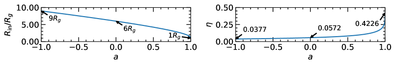
Figure 13: The ISCO radius $R_{\text{in}}$ (left panel) and radiative efficiency $\eta$ (right panel) compared to the dimensionless black hole spin $a$ calculated with Equations (A3) and (10) respectively. The values for $a=1$ (maximally prograde), $a=0$ (non-rotating), and $a=-1$ (maximally retrograde) are displayed by the arrows.

Appendix B Impact of parameters on transfer functions

Figure 14 presents the time delays and standard deviation differences between the $g$ and $i$ bands of the transfer functions as each parameter is varied. The mean time delay reflects the relative shift between the two bands, while the standard deviation affects the relative smoothness of the signal. We focus on the differences between the bands since only variations in time delay or smoothness are observable. This figure highlights the influence of each parameter on the observed variability; however, changes in the mean brightness of each band coming from modeling the spectrum helps to break some parameter degeneracies. It is apparent that the black hole mass has the largest effect, followed by the Eddington ratio, redshift, and temperature slope.

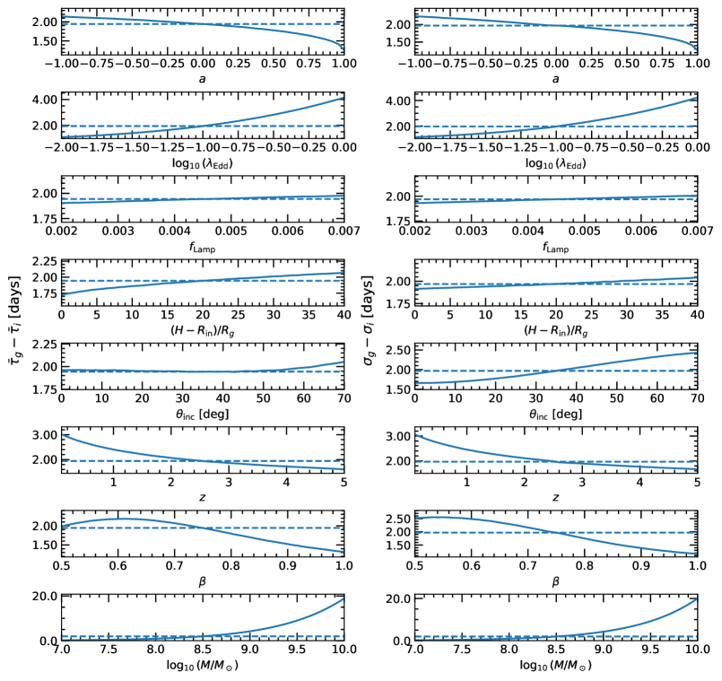
Figure 14: Time delays (left panels) and standard deviation (right panels) between the $g$ and $i$ bands alternating each parameter of our accretion disk simulation while the other parameters remain fixed at the mean values of the prior (see uniform priors in Table 1). The horizontal dashed line indicated the time delay and standard deviation when all the parameters are fixed to the mean values of the prior.

Appendix C Gaussian Process Regression Baseline

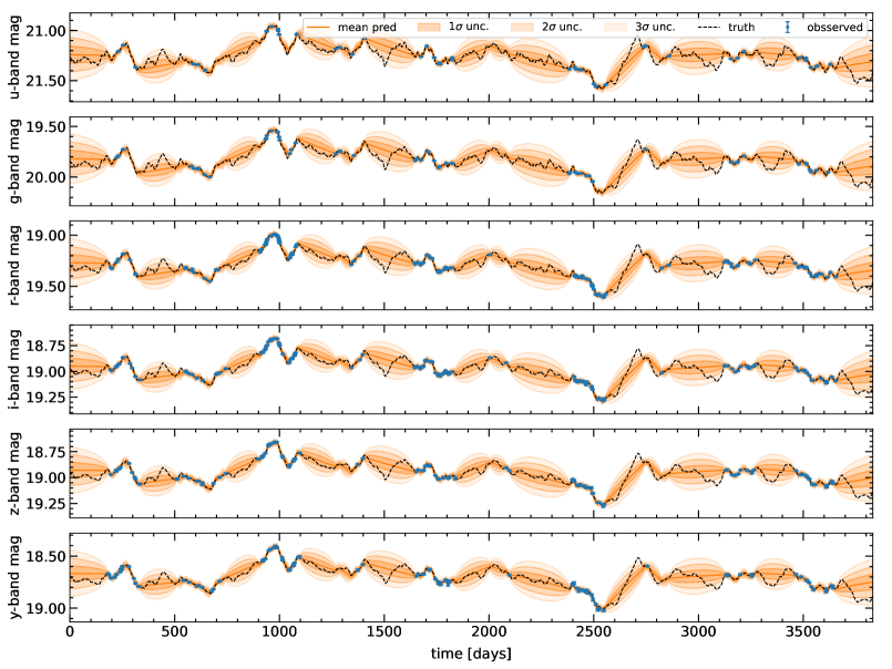
Figure 15: Same as Figure 6 for the UV/optical light curve reconstruction but using the multitask GPR baseline.

We compare the performance of our model to an exact, multitask GPR baseline (Maddox et al., 2021), the same as in Fagin et al. (2024b). The multitask GPR model infers correlation between the different features of the multivariate time series, in our case the different LSST wavebands, using an intrinsic co-regionalization model (ICM; Bonilla et al., 2007; Swersky et al., 2013). This is important since each band is highly correlated based on the same X-ray driving signal, and all observations should be used to inform the light curve reconstruction simultaneously. The noise-level of each observation is known, so we use the fixed-noise multitask GPR implemented in BoTorch (Balandat et al., 2020). We use an absolute exponential kernel, sometimes referred to as the Matérn-1/2 kernel, that is consistent with a DRW process. We note that although our light curves are not a DRW process, it has been imperially shown to best fit UV/optical quasar variability (Griffiths et al., 2021). We normalize each waveband of the light curve to have mean zero and variance one before fitting the GP. An example reconstructed UV/optical light curve is shown in Figure 15.

Appendix D Robustness test

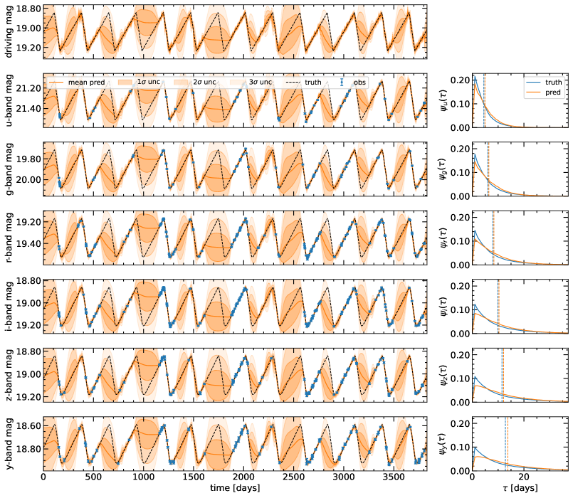
Figure 16: Same as Figure 6 but applying our pretrained machine learning model to a test light curve with sawtooth driving signal instead of a bended broken power-law.

Figure 17: Same as Figure 9 for the black hole mass but with applying the pretrained model to light curves with different out-of-distribution driving signals. The nominal test case of the broken power-law used to train the model is given in the top left panel.

To test the robustness of our trained network to out-of-distribution variability, we compare the performance of our model to test sets of light curves with BPL, DRW, BPL+Sine, Sine, sawtooth, and square wave driving signals. The BPL is our nominal test set and uses the same parameter range as our training set and is given in Table 1. The DRW is the same as the BPL but with $\alpha_{L}=0$ and $\alpha_{H}=2$, which we note is outside the parameter range of our training set. We use a Sine function with period $\log_{10}(T)\in[1,3]$. For the Sine+BPL, there is an additional parameter to determine the relative amplitude of the BPL, selected in the range of $[0.1,2.0]$. The sawtooth has period $\log_{10}(T)\in[1,3]$ with a relative width between each saw edge chosen between $[0,1]$ such that we have anything between a left and right facing right triangle. The square wave also has period $\log_{10}(T)\in[1,3]$ with relative width of each rectangular pulse chosen between $[0.1,0.9]$. We also randomize the phase of each periodic signal. We show an example reconstruction of a light curve with sawtooth driving variability in Figure 16. Despite the power spectrum of a sawtooth wave being very different than a broken power-law (it should be spiked near the frequency of the wave since it is periodic), our model still fits the observations and the signal is contained within the predicted $2\sigma$ credible interval. Since our model is trained using only stochastic signals, it will not recognize that this light curve is actually periodic, but is still able to reconstruct the accretion disk parameters and time delays between wavebands.

We compare the black hole mass predictions of our model with the different driving signal test sets in Figure 17. While here we demonstrate our network can still predict the black hole mass, our model can estimate the other accretion disk parameters similarly to Figure 9, including predicting the redshift, temperature slope, and Eddington ratio. Furthermore, it can still infer the time delays between wavebands. Thus our model is robust to different forms of out-of-distribution variability.

Appendix E Example parameter posterior and median predictions

Figure 18: Example of a posterior of the parameter predictions for the same test light curve shown in Figure 6. The diagonal elements display marginal distributions with the median and 1$\sigma$ levels indicated by dashed lines. The central elements depict 1$\sigma$, 2$\sigma$, and 3$\sigma$ contour levels. The true parameter values are overlaid in blue. The posterior is restricted to within the prior of each parameter by taking the sigmoid of the Gaussian mixture model and scaling back to its physical range.

Figure 19: Examples of median parameter predictions and $1\sigma$ confidence intervals for 100 random light curves in our nominal test set. The black dashed lines across the diagonal represent the ideal case where the median matches the true value of each parameter.

Figure 18 shows an example predicted parameter posterior from our network. Figure 19 shows an example of 100 different median and 1$\sigma$ confidence levels compared to the true values, demonstrating that larger uncertainties are predicted to compensate when the median is far from the true value.

References

- Abramowicz et al. (1988) Abramowicz, M. A., Czerny, B., Lasota, J. P., & Szuszkiewicz, E. 1988, The Astrophysical Journal, 332, 646, doi: 10.1086/166683
- Abramowicz & Fragile (2013) Abramowicz, M. A., & Fragile, P. C. 2013, Living Reviews in Relativity, 16, doi: 10.12942/lrr-2013-1
- Adam et al. (2022) Adam, A., Perreault-Levasseur, L., & Hezaveh, Y. 2022, Pixelated Reconstruction of Gravitational Lenses using Recurrent Inference Machines. https://arxiv.org/abs/2207.01073
- Agol & Krolik (2000) Agol, E., & Krolik, J. H. 2000, The Astrophysical Journal, 528, 161, doi: 10.1086/308177
- Arevalo et al. (2023) Arevalo, P., Churazov, E., Lira, P., et al. 2023, The universal power spectrum of Quasars in optical wavelengths: Break timescale scales directly with both black hole mass and accretion rate. https://arxiv.org/abs/2306.11099
- Astropy Collaboration et al. (2018) Astropy Collaboration, Price-Whelan, A. M., Sipőcz, B. M., et al. 2018, AJ, 156, 123, doi: 10.3847/1538-3881/aabc4f
- Ba et al. (2016) Ba, J. L., Kiros, J. R., & Hinton, G. E. 2016, Layer Normalization, arXiv, doi: 10.48550/ARXIV.1607.06450
- Bañados et al. (2018) Bañados, E., Venemans, B. P., Mazzucchelli, C., et al. 2018, Nature, 553, 473, doi: 10.1038/nature25180
- Balandat et al. (2020) Balandat, M., Karrer, B., Jiang, D. R., et al. 2020, in Advances in Neural Information Processing Systems 33. http://arxiv.org/abs/1910.06403
- Baydin et al. (2018) Baydin, A. G., Pearlmutter, B. A., Radul, A. A., & Siskind, J. M. 2018, Automatic differentiation in machine learning: a survey. https://arxiv.org/abs/1502.05767
- Best et al. (2024a) Best, H., Fagin, J., Vernardos, G., & O’Dowd, M. 2024a, Monthly Notices of the Royal Astronomical Society, 531, 1095, doi: 10.1093/mnras/stae1182
- Best et al. (2024b) Best, H., O’Dowd, M., Fagin, J., Chan, J. H. H., & Ierace, B. 2024b, Amoeba: An AGN Model of Optical Emissions Beyond steady-state Accretion discs. https://arxiv.org/abs/2410.19630
- Betancourt (2018) Betancourt, M. 2018, A Conceptual Introduction to Hamiltonian Monte Carlo. https://arxiv.org/abs/1701.02434
- Bhattacharyya et al. (2001) Bhattacharyya, S., Misra, R., & Thampan, A. V. 2001, The Astrophysical Journal, 550, 841, doi: 10.1086/319807
- Blackburne et al. (2015) Blackburne, J. A., Kochanek, C. S., Chen, B., Dai, X., & Chartas, G. 2015, ApJ, 798, 95, doi: 10.1088/0004-637X/798/2/95
- Blandford & Begelman (1999) Blandford, R. D., & Begelman, M. C. 1999, Monthly Notices of the Royal Astronomical Society, 303, L1, doi: 10.1046/j.1365-8711.1999.02358.x
- Blandford & McKee (1982) Blandford, R. D., & McKee, C. F. 1982, ApJ, 255, 419, doi: 10.1086/159843
- Bonilla et al. (2007) Bonilla, E. V., Chai, K., & Williams, C. 2007, in Advances in Neural Information Processing Systems, ed. J. Platt, D. Koller, Y. Singer, & S. Roweis, Vol. 20 (Curran Associates, Inc.). https://proceedings.neurips.cc/paper_files/paper/2007/file/66368270ffd51418ec58bd793f2d9b1b-Paper.pdf
- Brandt et al. (2018) Brandt, W., Ni, Q., Yang, G., et al. 2018, arXiv preprint arXiv:1811.06542
- Bursa (2017) Bursa, M. 2017, in RAGtime 17-19: Workshops on Black Holes and Neutron Stars, 7–21
- Bursa (2018) Bursa, M. 2018, SIM5: Library for ray-tracing and radiation transport in general relativity, Astrophysics Source Code Library, record ascl:1811.011. http://ascl.net/1811.011
- Cackett et al. (2021) Cackett, E. M., Bentz, M. C., & Kara, E. 2021, iScience, 24, 102557, doi: 10.1016/j.isci.2021.102557
- Cackett et al. (2007) Cackett, E. M., Horne, K., & Winkler, H. 2007, MNRAS, 380, 669, doi: 10.1111/j.1365-2966.2007.12098.x
- Chan et al. (2024) Chan, J. H.-H., Fagin, J., Best, H., & O’Dowd, M. J. 2024, Reverberation Mapping of Lamp-post and Wind Structures in Accretion Thin Disks. https://arxiv.org/abs/2409.15669
- Che et al. (2016) Che, Z., Purushotham, S., Cho, K., Sontag, D., & Liu, Y. 2016, Recurrent Neural Networks for Multivariate Time Series with Missing Values, arXiv, doi: 10.48550/ARXIV.1606.01865
- Chung et al. (2014) Chung, J., Gulcehre, C., Cho, K., & Bengio, Y. 2014, Empirical Evaluation of Gated Recurrent Neural Networks on Sequence Modeling, arXiv, doi: 10.48550/ARXIV.1412.3555
- Collaboration et al. (2009) Collaboration, L. S., Abell, P. A., Allison, J., et al. 2009, LSST Science Book, Version 2.0. https://arxiv.org/abs/0912.0201
- Cornachione & Morgan (2020) Cornachione, M. A., & Morgan, C. W. 2020, The Astrophysical Journal, 895, 93, doi: 10.3847/1538-4357/ab8aed
- Cunningham & Bardeen (1973) Cunningham, C. T., & Bardeen, J. M. 1973, ApJ, 183, 237, doi: 10.1086/152223
- Czerny et al. (2023) Czerny, B., Panda, S., Prince, R., et al. 2023, A&A, 675, A163, doi: 10.1051/0004-6361/202345844
- Danilov et al. (2022) Danilov, E., Ćiprijanović, A., & Nord, B. 2022, Neural Inference of Gaussian Processes for Time Series Data of Quasars, arXiv, doi: 10.48550/ARXIV.2211.10305
- Fagin et al. (2024a) Fagin, J., Paic, E., Neira, F., et al. 2024a, Predicting High Magnification Events in Microlensed Quasars in the Era of LSST using Recurrent Neural Networks. https://arxiv.org/abs/2409.08999
- Fagin et al. (2024b) Fagin, J., Park, J. W., Best, H., et al. 2024b, The Astrophysical Journal, 965, 104, doi: 10.3847/1538-4357/ad2988
- Fausnaugh et al. (2018) Fausnaugh, M. M., Starkey, D. A., Horne, K., et al. 2018, ApJ, 854, 107, doi: 10.3847/1538-4357/aaaa2b
- Foreman-Mackey (2016) Foreman-Mackey, D. 2016, The Journal of Open Source Software, 1, 24, doi: 10.21105/joss.00024
- Foreman-Mackey et al. (2017) Foreman-Mackey, D., Agol, E., Angus, R., & Ambikasaran, S. 2017, ArXiv. https://arxiv.org/abs/1703.09710
- Franceschini et al. (1999) Franceschini, A., Hasinger, G., Miyaji, T., & Malquori, D. 1999, Monthly Notices of the Royal Astronomical Society, 310, L5, doi: 10.1046/j.1365-8711.1999.03078.x
- Greenstein (1963) Greenstein, J. L. 1963, Nature, 197, 1041, doi: 10.1038/1971041a0
- Griffiths et al. (2021) Griffiths, R.-R., Jiang, J., Buisson, D. J. K., et al. 2021, The Astrophysical Journal, 914, 144, doi: 10.3847/1538-4357/abfa9f
- Guo et al. (2022) Guo, W.-J., Li, Y.-R., Zhang, Z.-X., Ho, L. C., & Wang, J.-M. 2022, The Astrophysical Journal, 929, 19, doi: 10.3847/1538-4357/ac4e84
- Harris et al. (2020) Harris, C. R., Millman, K. J., van der Walt, S. J., et al. 2020, Nature, 585, 357–362, doi: 10.1038/s41586-020-2649-2
- Hazard et al. (1963) Hazard, C., Mackey, M. B., & Shimmins, A. J. 1963, Nature, 197, 1037, doi: 10.1038/1971037a0
- He et al. (2015) He, K., Zhang, X., Ren, S., & Sun, J. 2015, Deep Residual Learning for Image Recognition, arXiv, doi: 10.48550/ARXIV.1512.03385
- Hendrycks & Gimpel (2023) Hendrycks, D., & Gimpel, K. 2023, Gaussian Error Linear Units (GELUs). https://arxiv.org/abs/1606.08415
- Heydari-Fard et al. (2023) Heydari-Fard, M., Honarvar, S. G., & Heydari-Fard, M. 2023, Monthly Notices of the Royal Astronomical Society, 521, 708, doi: 10.1093/mnras/stad558
- Hoshi et al. (2024) Hoshi, A., Yamada, T., Kokubo, M., Matsuoka, Y., & Nagao, T. 2024, The Astrophysical Journal, 969, 11, doi: 10.3847/1538-4357/ad414c
- Huang et al. (2023) Huang, J., Feng, H., Gu, W.-M., & Wu, W.-B. 2023, Black Hole Accretion with Saturated Magnetic Pressure and Disk Wind. https://arxiv.org/abs/2307.06585
- Huber et al. (2021) Huber, S., Suyu, S. H., Noebauer, U. M., et al. 2021, A&A, 646, A110, doi: 10.1051/0004-6361/202039218
- Hunter (2007) Hunter, J. D. 2007, Computing in Science & Engineering, 9, 90, doi: 10.1109/MCSE.2007.55
- Ivezić et al. (2019) Ivezić, Ž., Kahn, S. M., Tyson, J. A., et al. 2019, ApJ, 873, 111, doi: 10.3847/1538-4357/ab042c
- Jha et al. (2022) Jha, V. K., Joshi, R., Chand, H., et al. 2022, Monthly Notices of the Royal Astronomical Society, 511, 3005, doi: 10.1093/mnras/stac109
- Kauffmann & Haehnelt (2000) Kauffmann, G., & Haehnelt, M. 2000, Monthly Notices of the Royal Astronomical Society, 311, 576, doi: 10.1046/j.1365-8711.2000.03077.x
- Kelly et al. (2009) Kelly, B. C., Bechtold, J., & Siemiginowska, A. 2009, in American Astronomical Society Meeting Abstracts, Vol. 213, American Astronomical Society Meeting Abstracts #213, 422.06
- Khadka & Ratra (2020) Khadka, N., & Ratra, B. 2020, Monthly Notices of the Royal Astronomical Society, 497, 263, doi: 10.1093/mnras/staa1855
- Kingma & Ba (2017) Kingma, D. P., & Ba, J. 2017, Adam: A Method for Stochastic Optimization. https://arxiv.org/abs/1412.6980
- Kingma & Welling (2013) Kingma, D. P., & Welling, M. 2013, Auto-Encoding Variational Bayes, arXiv, doi: 10.48550/ARXIV.1312.6114
- Kirkby et al. (2023) Kirkby, D., Robitaille, T., Weaver, B. A., et al. 2023, desihub/speclite: 2MASS Filters, v0.17, Zenodo, doi: 10.5281/zenodo.8347108
- Li et al. (2024) Li, J. I.-H., Johnson, S. D., Avestruz, C., et al. 2024, Fast and Flexible Inference Framework for Continuum Reverberation Mapping using Simulation-based Inference with Deep Learning. https://arxiv.org/abs/2407.14621
- Li et al. (2020) Li, X., Wong, T.-K. L., Chen, R. T. Q., & Duvenaud, D. 2020, International Conference on Artificial Intelligence and Statistics
- Li et al. (2018) Li, Y.-P., Yuan, F., & Dai, X. 2018, Monthly Notices of the Royal Astronomical Society, 483, 2275, doi: 10.1093/mnras/sty3245
- Luminet (1979) Luminet, J. P. 1979, A&A, 75, 228
- Maas et al. (2013) Maas, A. L., Hannun, A. Y., Ng, A. Y., et al. 2013, Rectifier nonlinearities improve neural network acoustic models
- MacLeod et al. (2010) MacLeod, C. L., Ivezić, Ž., Kochanek, C., et al. 2010, The Astrophysical Journal, 721, 1014
- Maddox et al. (2021) Maddox, W. J., Balandat, M., Wilson, A. G., & Bakshy, E. 2021, Bayesian Optimization with High-Dimensional Outputs, arXiv, doi: 10.48550/ARXIV.2106.12997
- Markowitz (2010) Markowitz, A. 2010, The Astrophysical Journal, 724, 26, doi: 10.1088/0004-637X/724/1/26
- Mastroserio et al. (2018) Mastroserio, G., Ingram, A., & van der Klis, M. 2018, Monthly Notices of the Royal Astronomical Society, 475, 4027, doi: 10.1093/mnras/sty075
- Matthews & Sandage (1963) Matthews, T. A., & Sandage, A. R. 1963, ApJ, 138, 30, doi: 10.1086/147615
- McHardy et al. (2004) McHardy, I. M., Papadakis, I. E., Uttley, P., Page, M. J., & Mason, K. O. 2004, Monthly Notices of the Royal Astronomical Society, 348, 783, doi: 10.1111/j.1365-2966.2004.07376.x
- Modi et al. (2021) Modi, C., Lanusse, F., Seljak, U., Spergel, D. N., & Perreault-Levasseur, L. 2021, CosmicRIM : Reconstructing Early Universe by Combining Differentiable Simulations with Recurrent Inference Machines. https://arxiv.org/abs/2104.12864
- Morgan et al. (2018) Morgan, C. W., Hyer, G. E., Bonvin, V., et al. 2018, ApJ, 869, 106, doi: 10.3847/1538-4357/aaed3e
- Morningstar et al. (2019) Morningstar, W. R., Levasseur, L. P., Hezaveh, Y. D., et al. 2019, The Astrophysical Journal, 883, 14, doi: 10.3847/1538-4357/ab35d7
- Mortlock et al. (2011) Mortlock, D. J., Warren, S. J., Venemans, B. P., et al. 2011, Nature, 474, 616, doi: 10.1038/nature10159
- Mudd et al. (2018) Mudd, D., Martini, P., Zu, Y., et al. 2018, ApJ, 862, 123, doi: 10.3847/1538-4357/aac9bb
- Muñoz et al. (2016) Muñoz, J. A., Vives-Arias, H., Mosquera, A. M., et al. 2016, The Astrophysical Journal, 817, 155, doi: 10.3847/0004-637x/817/2/155
- Novikov & Thorne (1973) Novikov, I. D., & Thorne, K. S. 1973, in Black Holes (Les Astres Occlus), 343–450
- Oke (1963) Oke, J. B. 1963, Nature, 197, 1040, doi: 10.1038/1971040b0
- O’Neill et al. (2005) O’Neill, P. M., Nandra, K., Papadakis, I. E., & Turner, T. J. 2005, Monthly Notices of the Royal Astronomical Society, 358, 1405, doi: 10.1111/j.1365-2966.2005.08860.x
- Panda et al. (2019) Panda, S., Martínez-Aldama, M. L., & Zajaček, M. 2019, Frontiers in Astronomy and Space Sciences, 6, doi: 10.3389/fspas.2019.00075
- Papoutsis et al. (2024) Papoutsis, M., Papadakis, I. E., Panagiotou, C., Dovčiak, M., & Kammoun, E. 2024, X-ray reverberation as an explanation for UV/optical variability in nearby Seyferts. https://arxiv.org/abs/2409.10417
- Park et al. (2021) Park, J. W., Villar, A., Li, Y., et al. 2021, Inferring Black Hole Properties from Astronomical Multivariate Time Series with Bayesian Attentive Neural Processes, arXiv, doi: 10.48550/ARXIV.2106.01450
- Paszke et al. (2019) Paszke, A., Gross, S., Massa, F., et al. 2019, in Advances in Neural Information Processing Systems 32 (Curran Associates, Inc.), 8024–8035
- Poindexter & Kochanek (2010) Poindexter, S., & Kochanek, C. S. 2010, ApJ, 712, 668, doi: 10.1088/0004-637X/712/1/668
- Poindexter et al. (2008) Poindexter, S., Morgan, N., & Kochanek, C. S. 2008, ApJ, 673, 34, doi: 10.1086/524190
- Prša et al. (2023) Prša, A., Yoachim, P., & Jones, L. 2023, ApJS, 267, 22, doi: 10.3847/1538-4365/acda31
- Putzky & Welling (2017) Putzky, P., & Welling, M. 2017, Recurrent Inference Machines for Solving Inverse Problems. https://arxiv.org/abs/1706.04008
- Rasmussen & Williams (2006) Rasmussen, C. E., & Williams, C. K. I. 2006, Gaussian processes for machine learning., Adaptive computation and machine learning (MIT Press), I–XVIII, 1–248
- Rezende et al. (2014) Rezende, D. J., Mohamed, S., & Wierstra, D. 2014, in International conference on machine learning, PMLR, 1278–1286
- Rhea et al. (2023) Rhea, C., Hlavacek-Larrondo, J., Kraft, R., et al. 2023, Unraveling the Mysteries of Galaxy Clusters: Recurrent Inference Deconvolution of X-ray Spectra. https://arxiv.org/abs/2311.18014
- Salpeter (1964) Salpeter, E. E. 1964, ApJ, 140, 796, doi: 10.1086/147973
- Sá nchez-Sáez et al. (2021) Sá nchez-Sáez, P., Lira, H., Martí, L., et al. 2021, The Astronomical Journal, 162, 206, doi: 10.3847/1538-3881/ac1426
- Sartori et al. (2019) Sartori, L. F., Trakhtenbrot, B., Schawinski, K., et al. 2019, The Astrophysical Journal, 883, 139, doi: 10.3847/1538-4357/ab3c55
- Schirmer et al. (2022) Schirmer, M., Eltayeb, M., Lessmann, S., & Rudolph, M. 2022, Modeling Irregular Time Series with Continuous Recurrent Units. https://arxiv.org/abs/2111.11344
- Schmidt (1963) Schmidt, M. 1963, Nature, 197, 1040, doi: 10.1038/1971040a0
- Secunda et al. (2024) Secunda, A., Greene, J. E., Jiang, Y.-F., Yao, P. Z., & Zoghbi, A. 2024, Negative Lags on the Viscous Timescale in Quasar Photometry and Prospects for Detecting More with LSST. https://arxiv.org/abs/2306.05455
- Shakura & Sunyaev (1973) Shakura, N. I., & Sunyaev, R. A. 1973, A&A, 24, 337
- Sheng et al. (2022) Sheng, X., Ross, N., & Nicholl, M. 2022, Monthly Notices of the Royal Astronomical Society, 512, 5580, doi: 10.1093/mnras/stac803
- Starkey et al. (2015) Starkey, D. A., Horne, K., & Villforth, C. 2015, Monthly Notices of the Royal Astronomical Society, 456, 1960, doi: 10.1093/mnras/stv2744
- Suberlak et al. (2021) Suberlak, K. L., Ivezić, Ž ., & MacLeod, C. 2021, The Astrophysical Journal, 907, 96, doi: 10.3847/1538-4357/abc698
- Summons (2007) Summons, D. P. 2007, PhD thesis, University of Southampton. https://eprints.soton.ac.uk/466440/
- Sun et al. (2018) Sun, M., Xue, Y., Trump, J. R., & Gu, W.-M. 2018, Monthly Notices of the Royal Astronomical Society, 482, 2788, doi: 10.1093/mnras/sty2885
- Swersky et al. (2013) Swersky, K., Snoek, J., & Adams, R. P. 2013, in Advances in Neural Information Processing Systems, ed. C. Burges, L. Bottou, M. Welling, Z. Ghahramani, & K. Weinberger, Vol. 26 (Curran Associates, Inc.). https://proceedings.neurips.cc/paper_files/paper/2013/file/f33ba15effa5c10e873bf3842afb46a6-Paper.pdf
- Tachibana et al. (2020) Tachibana, Y., Graham, M. J., Kawai, N., et al. 2020, The Astrophysical Journal, 903, 54, doi: 10.3847/1538-4357/abb9a9
- Temple et al. (2021) Temple, M. J., Hewett, P. C., & Banerji, M. 2021, Monthly Notices of the Royal Astronomical Society, 508, 737, doi: 10.1093/mnras/stab2586
- Timmer & Koenig (1995) Timmer, J., & Koenig, M. 1995, A&A, 300, 707
- Ursini et al. (2020) Ursini, F., Dovčiak, M., Zhang, W., et al. 2020, A&A, 644, A132, doi: 10.1051/0004-6361/202039158
- Uttley & McHardy (2005) Uttley, P., & McHardy, I. M. 2005, Monthly Notices of the Royal Astronomical Society, 363, 586, doi: 10.1111/j.1365-2966.2005.09475.x
- Vaswani et al. (2023) Vaswani, A., Shazeer, N., Parmar, N., et al. 2023, Attention Is All You Need. https://arxiv.org/abs/1706.03762
- Vernardos & Tsagkatakis (2019) Vernardos, G., & Tsagkatakis, G. 2019, Monthly Notices of the Royal Astronomical Society, 486, 1944, doi: 10.1093/mnras/stz868
- Virtanen et al. (2020) Virtanen, P., Gommers, R., Oliphant, T. E., et al. 2020, Nature Methods, 17, 261, doi: 10.1038/s41592-019-0686-2
- Wagner-Carena et al. (2021) Wagner-Carena, S., Park, J. W., Birrer, S., et al. 2021, The Astrophysical Journal, 909, 187, doi: 10.3847/1538-4357/abdf59
- Wang et al. (2023) Wang, S., Guo, H., & Woo, J.-H. 2023, The Astrophysical Journal Letters, 948, L23, doi: 10.3847/2041-8213/accf96
- Wong et al. (2019) Wong, K. C., Suyu, S. H., Chen, G. C.-F., et al. 2019, Monthly Notices of the Royal Astronomical Society, 498, 1420, doi: 10.1093/mnras/stz3094
- Yang et al. (2022) Yang, H., Jin, C., & Yuan, W. 2022, The Astrophysical Journal, 936, 36, doi: 10.3847/1538-4357/ac83bb
- Yao et al. (2023) Yao, P. Z., Secunda, A., Jiang, Y.-F., Greene, J. E., & Villar, A. 2023, The Astrophysical Journal, 953, 43, doi: 10.3847/1538-4357/acde7e
- You et al. (2016) You, B., Straub, O., Czerny, B., et al. 2016, The Astrophysical Journal, 821, 104, doi: 10.3847/0004-637x/821/2/104
- Yu et al. (2022) Yu, W., Richards, G. T., Vogeley, M. S., Moreno, J., & Graham, M. J. 2022, The Astrophysical Journal, 936, 132, doi: 10.3847/1538-4357/ac8351
- Yuk et al. (2023) Yuk, H., Dai, X., Jayasinghe, T., et al. 2023, Correlation Between Optical and X-ray Break Frequencies in Power Spectra of Active Galactic Nuclei. https://arxiv.org/abs/2306.17334
- Zel’dovich (1964) Zel’dovich, Y. B. 1964, Soviet Physics Doklady, 9, 195
- Zu et al. (2013) Zu, Y., Kochanek, C. S., Kozłowski, S., & Udalski, A. 2013, The Astrophysical Journal, 765, 106, doi: 10.1088/0004-637x/765/2/106
- Zu et al. (2016) Zu, Y., Kochanek, C. S., Kozłowski, S., & Peterson, B. M. 2016, The Astrophysical Journal, 819, 122, doi: 10.3847/0004-637x/819/2/122
- Zu et al. (2011) Zu, Y., Kochanek, C. S., & Peterson, B. M. 2011, The Astrophysical Journal, 735, 80, doi: 10.1088/0004-637X/735/2/80
- Čvorović Hajdinjak et al. (2022) Čvorović Hajdinjak, I., Kovačević, A. B., Ilić, D., et al. 2022, Astronomische Nachrichten, 343, e210103, doi: https://doi.org/10.1002/asna.20210103