A Causal Graph-Enhanced Gaussian Process Regression for Modeling Engine-out NOx

Abstract

The stringent regulatory requirements on nitrogen oxides (NOx) emissions from diesel compression ignition engines require accurate and reliable models for real-time monitoring and diagnostics. Although traditional methods such as physical sensors and virtual engine control module (ECM) sensors provide essential data, they are only used for estimation. Ubiquitous literature primarily focuses on deterministic models with little emphasis on capturing the uncertainties due to sensors. The lack of probabilistic frameworks restricts the applicability of these models for robust diagnostics. The objective of this paper is to develop and validate a probabilistic model to predict engine-out NOx emissions using Gaussian process regression. Our approach is as follows. We employ three variants of Gaussian process models: the first with a standard radial basis function kernel with input window, the second incorporating a deep kernel using convolutional neural networks to capture temporal dependencies, and the third enriching the deep kernel with a causal graph derived via graph convolutional networks. The causal graph embeds physics knowledge into the learning process. All models are compared against a virtual ECM sensor using both quantitative and qualitative metrics. We conclude that our model provides an improvement in predictive performance when using an input window and a deep kernel structure. Even more compelling is the further enhancement achieved by the incorporation of a causal graph into the deep kernel. These findings are corroborated across different validation datasets.

1 Introduction

Given the detrimental impact of nitrogen oxides (NOx) on environmental and human health, stringent regulations (EPA, 2021) are essential to mitigate these effects and ensure sustainable urban air quality. In this context, developing robust predictive models is crucial for guiding the evolution of internal combustion engine technology, enabling manufacturers to comply with evolving global environmental legislation and effectively reducing air pollutants, including those contributing to greenhouse gas emissions. Research on predictive models for engine-out NOx emissions remains a dynamic and ongoing area of focus within the diesel powertrain research community. Although extensive research in this field is documented in the open literature (Aliramezani et al., 2022), more studies need to be conducted to address the uncertainty analysis of these models. These models are typically designed for real-time implementation, and the model prediction is often used for control or diagnostic purposes. Consequently, it is essential to develop probabilistic models that not only forecast emissions but also specify expected error margins or define an error probability distribution.

Given the extensive research on modeling engine-out NOx, various methods have been explored to address the complexities and uncertainties inherent in these systems. Traditional physics-based models have been developed to capture the underlying mechanisms of NOx formation in diesel engines. For instance Asprion et al. (2013) proposed a fast and accurate physics-based model for NOx. Similarly Aithal (2010) used finite-rate chemical kinetics to model NOx formation in diesel engines, highlighting the role of combustion processes. These models, while insightful, often require extensive computational resources and detailed knowledge of engine parameters. In contrast, data-driven approaches have gained popularity due to their ability to learn from empirical data and predict NOx emissions with high accuracy.  Fang et al. (2022) used artificial neural networks to predict transient NOx emissions from high-speed direct injection diesel engines. Similarly  Shin et al. (2020) developed a deep neural network model with Bayesian hyperparameter optimization to predict NOx emissions under transient conditions. Other studies have also used support vector machines and particle swarm optimization for emission modeling in homogeneous charge compression ignition engines (Gordon et al., 2023). Hybrid approaches that combine physical insights with machine learning techniques have also been explored. For instance, Shahpouri et al. (2021) investigated hybrid ML methods for soot emission prediction. However, these deterministic models often overlook the uncertainties associated with sensor data and engine dynamics. To address this limitation, probabilistic frameworks have been proposed. Yousefian et al. (2021) applied Bayesian inference and uncertainty quantification to hydrogen-enriched and lean-premixed combustion systems. Cho et al. (2018) presented a structured approach to uncertainty analysis of predictive models for engine-out NOx, highlighting the need for robust uncertainty quantification.

Gaussian processes (GPs) (Williams and Rasmussen, 2006) are widely used in Bayesian modeling due to their interpretability and robust ability to quantify uncertainty. Typically, GPs rely on a small number of kernel hyperparameters, which are optimized based on the marginal likelihood. However, in most common scenarios, the kernel is fixed, which limits the GP’s ability to adaptively learn from data in a way that could improve predictive performance. This leads to GP primarily acting as smoothing mechanisms, which can be a constraint when dealing with complex, high-dimensional data. On the other hand, deep neural networks (LeCun et al., 2015) are known for their powerful representation learning capabilities, enabling them to make predictions on unseen test data. Despite their success, standard deterministic neural networks often produce overconfident predictions (Guo et al., 2017) and struggle with providing reliable uncertainty estimates. Bayesian neural networks (BNNs) have been proposed to address these limitations, but inference in BNNs remains challenging due to the complex posterior distributions and the large number of parameters involved. Furthermore, BNNs often require multiple forward passes to obtain an estimate of the predictive posterior, increasing computational costs. Given these issues, it is appealing to combine the uncertainty quantification strengths of GPs with the representation learning power of neural networks. This led to the development of deep kernel learning (DKL) (Wilson et al., 2016), which uses a neural network to learn representations from data and then inputs these representations into a GP. This approach allows for joint end-to-end training of both the kernel and network parameters, either through variational inference or marginal likelihood optimization. In Wilson et al. (2016), DKL has demonstrated superior performance compared to traditional kernel methods, such as the radial basis function (RBF) kernel, as well as standard neural networks, across a variety of tasks.

Graph neural networks (GNNs) have emerged as a powerful tool for learning from graph-structured data, evolving through several stages to address increasingly complex data representation and learning tasks. The inception of GNNs (Scarselli et al., 2008) marked a significant shift in how data structured in graphs could be processed by learning algorithms. Graph convolutional networks (GCNs) (Kipf and Welling, 2016a) introduced the concept of applying convolutional operations directly on graphs. These networks extend the convolutional paradigm to graph data by considering the graph’s structure in the convolution operation, allowing for the aggregation of neighbor features through a form of weighted average. This approach effectively captures local graph structures and node features, leading to improved performance in tasks such as node classification and graph classification. Building on the success of GCNs, graph attention networks (Veličković et al., 2017) introduced an attention mechanism that allows nodes to weigh the importance of their neighbors’ information dynamically. This mechanism allows the model to focus more on relevant parts of the graph, improving the model’s ability to learn from complex graph structures. GATs have shown significant improvements in various tasks by allowing more nuanced feature aggregation from neighbors, compared to the more uniform aggregation in GCNs. Gated graph sequence networks (GGSNs) (Li et al., 2015) represent a further evolution in the processing of graph-structured data, incorporating elements of sequence modeling into graph networks. By using gated recurrent units (Zinage et al., 2024b) or similar mechanisms, GGSNs can model graph dynamics and temporal changes, making them particularly suited for tasks involving sequences of graphs or graphs with evolving structures. This approach has expanded the applicability of GNNs to a broader range of tasks, including those that involve time-series data on graphs. Variational graph autoencoders (VGAEs) (Kipf and Welling, 2016b) also represent a key development in unsupervised learning for graph-structured data, extending the idea of autoencoders with a probabilistic framework. VGAEs use an encoder-decoder structure where the encoder maps nodes into a latent space, learning distributions over latent variables instead of fixed embeddings. This probabilistic approach allows VGAEs to capture uncertainty in the node representations, making the model more robust in learning from sparse or noisy graph data. After generating the latent distributions, the decoder reconstructs the graph’s adjacency matrix by sampling from these distributions and calculating the likelihood of edges between nodes. VGAEs have been particularly effective in tasks like link prediction and graph generation, where understanding the inherent uncertainty in graph structures is important. Graph isomorphism networks (GINs) (Xu et al., 2018) further push the boundaries of GNNs by improving their ability to differentiate between distinct graph structures. GINs are as powerful as the Weisfeiler-Lehman test for graph isomorphism, which determines whether two graphs are structurally identical. By using a sum operation to aggregate neighbor features, GINs ensure that even subtle differences in graph topology are captured. This makes GINs particularly effective in graph classification tasks, where minor structural variations can significantly affect outcomes.

The primary contribution of this work is the incorporation of causal information within the deep kernel structure using GCNs. This causal information derived from the causal graph serves to embed physics-informed knowledge into the learning process.

We have organized our paper as follows. We begin by delving into the physical principles underlying the formation of NOx. Next, we discuss Gaussian process regression (GPR). Following this, we detail the findings of our study. Finally, the conclusions are succinctly presented.

This research has been conducted in collaboration with Cummins Inc with the data from a Cummins medium-duty diesel engine. In compliance with Cummins policies, all plots in this study have been normalized.

2 Engine-out $\mathrm{NO}_{x}$ formation

The formation of $\mathrm{NO}_{x}$, consisting of nitric oxide ($\mathrm{NO}$) and nitrogen dioxide ($\mathrm{NO}_{2}$), in diesel engines involves several mechanisms. Notably, thermal $\mathrm{NO}$, fuel $\mathrm{NO}$, and prompt $\mathrm{NO}$ play crucial roles (Heywood, 2018). Prompt $\mathrm{NO}$ predominantly forms under fuel-rich conditions and exhibits minimal temperature dependency. Conversely, fuel $\mathrm{NO}$ relies on nitrogenous compounds in the fuel. The dominant process in diesel engines for $\mathrm{NO}$ generation within the combustion chamber is thermal $\mathrm{NO}$, as described by the extended Zeldovich mechanism (Lavoie et al., 1970). This process results from the oxidation of atmospheric nitrogen. The key reactions for thermal $\mathrm{NO}$ are as follows:

$$\begin{split}\mathrm{N}_{2}+\mathrm{O}\rightarrow\mathrm{NO}+\mathrm{N},\\ \mathrm{N}+\mathrm{O}_{2}\rightarrow\mathrm{NO}+\mathrm{O},\\ \mathrm{N}+\mathrm{OH}\rightarrow\mathrm{NO}+\mathrm{H}.\end{split}$$

These reactions are very sensitive to combustion temperature (exceeding $2000\mathrm{~{}K}$), in-cylinder oxygen ($\mathrm{O}_{2}$) levels, and the duration at peak temperatures within lean air-fuel mixtures (Bowman, 1975). In contrast, $\mathrm{NO}_{2}$ formation primarily occurs downstream of the cylinder through incomplete oxidation of $\mathrm{NO}$, explained by the reaction:

$$\mathrm{NO}+\mathrm{HO}_{2}\rightarrow\mathrm{NO}_{2}+\mathrm{OH}.$$

Engine-out $\mathrm{NO}_{x}$ levels are largely governed by the temperature of the burnt gases and $\mathrm{O}_{2}$ concentration. These factors are influenced by various engine parameters, such as intake air mass flow rate, fuel flow rate along with engine speed and load. Consequently, these engine variables are chosen for modeling engine-out $\mathrm{NO}_{x}$. An effective method for controlling engine-out $\mathrm{NO}_{x}$ in diesel engines is exhaust gas recirculation (EGR). EGR predominantly consists of nitrogen ($\mathrm{N}_{2}$), carbon dioxide ($\mathrm{CO}_{2}$), and water vapor ($\mathrm{H}_{2}\mathrm{O}$), which displaces air in the cylinder and leads to reduced $\mathrm{NO}_{x}$ formation. The decrease in $\mathrm{NO}_{x}$ is attributed to the lowered oxygen concentration and combustion temperatures due to the higher specific heat capacity of the triatomic molecules present in EGR.

3 Gaussian Process Regression

GP is a probabilistic non-parametric approach which defines a prior over functions and can be used for regression tasks. A GP is exhaustively described by its mean function, $m(\boldsymbol{x})$, and a covariance function known as the kernel function, $k(\boldsymbol{x},\boldsymbol{x}^{\prime})$. Importantly, for any finite set of inputs, a GP will output a multivariate Gaussian distribution. In the context of GPR, the underlying assumption is that the function to be approximated is a sample from a GP.

The mean function, $m(\boldsymbol{x})$, and covariance function $k(\boldsymbol{x},\boldsymbol{x}^{\prime})$, are represented by the equations:

$$m(\boldsymbol{x}) =\mathbb{E}[f(\boldsymbol{x})],$$

$$k(\boldsymbol{x},\boldsymbol{x}^{\prime}) =\mathbb{E}[(f(\boldsymbol{x})-m(\boldsymbol{x}))(f(\boldsymbol{x}^{\prime})-m(\boldsymbol{x}^{\prime}))].$$

In practice, it is common to use a zero mean function, i.e., $m(\boldsymbol{x})=0$, and focus on defining the covariance function. The covariance function, measures the similarity between data points. One common choice is the radial basis function (RBF) kernel with automatic relevance determination (ARD). Assuming $l_{d}$ represents the length scale for each dimension, and $D$ indicates the number of dimensions, we have:

$$k_{\alpha}^{\text{rbf}}(\boldsymbol{x},\boldsymbol{x}^{\prime})=\sigma^{2}\exp\left(-\sum_{d=1}^{D}\frac{(x_{d}-x^{\prime}_{d})^{2}}{2l_{d}^{2}}\right),$$

where $\sigma^{2}$ is the signal variance and $\alpha=(l_{1},l_{2},\ldots l_{d},\sigma^{2})$. The length scales $l_{d}$ control the relevance of different dimensions. When $l_{d}$ is small, changes in the $d$-th dimension have a large effect on the covariance, making that dimension more relevant.

Given a dataset $\mathcal{D}$ of $n$ input vectors, $X=\left(\mathbf{x}_{1},\ldots,\mathbf{x}_{n}\right)$, each having dimension $D$, these index an $n\times 1$ vector of targets $\mathbf{y}=\left(y_{1},\ldots,y_{n}\right)$. Assuming the presence of additive Gaussian noise, the relationship between the likelihood functions is:

$$y_{i}\mid f(\mathbf{x}_{i})\sim\mathcal{N}\left(y_{i};f(\mathbf{x}_{i}),\sigma_{y}^{2}\right),$$

where $\sigma_{y}^{2}$ is the variance of the noise. The observations are assumed to be independent. The predictive distribution of the GP at $n_{*}$ test points indexed by $X_{*}$ can then be expressed as:

where,

$$\mathbf{f}_{*}=f_{*}(X)=\left[f_{*}\left(\mathbf{x}_{1}\right),\ldots,f_{*}\left(\mathbf{x}_{n}\right)\right]^{\top}.$$

Here, $k_{\theta}(X_{*},X)$ is an $n_{*}\times n$ matrix of covariances between the GP evaluated at $X_{*}$ and $X$. Additionally, $m(X_{*})$ designates the $n_{*}\times 1$ mean vector, and $k_{\theta}(X,X)$ represents the $n\times n$ covariance matrix evaluated at training inputs $X$. The conditional probability density of the target variable $\mathbf{y}$, given the parameters $\theta$ and input data $X$, can be expressed as:

$$\begin{split}\log p(\mathbf{y}\mid\theta,X)\propto-\Bigg{[}\overbrace{\mathbf{y}^{\top}\left(k_{\theta}(X,X)+\sigma_{y}^{2}I\right)^{-1}\mathbf{y}}^{\text{model fit}}\,+\\ \underbrace{\log\left|k_{\theta}(X,X)+\sigma_{y}^{2}I\right|}_{\text{complexity penalty}}\Bigg{]}.\end{split}$$

The parameters $\theta$ are found by maximizing this quantity.

3.1 Deep kernel

A deep kernel (Wilson et al., 2016; Zinage et al., 2024a) integrates a neural network with a traditional kernel function, improving the model’s ability to capture complex patterns in data. The neural network effectively compresses and distills the input space, mapping it to a lower-dimensional representation that is more informative for the GP model. The transformation induced by the neural network can allow the model to fit more complicated, non-smooth, and anisotropic functions, unlike the standard kernels like RBF, which model smooth and isotropic functions (Calandra et al., 2016). Also, by mapping a high-dimensional input space to a lower-dimensional one using a neural network, we can mitigate the curse of dimensionality. This makes the GPR more tractable and can improve its generalization by focusing on the most informative dimensions of the data.

Figure 1: Deep kernel using CNN

Assuming $\phi(\boldsymbol{x};\boldsymbol{w})$ is a nonlinear mapping given by a neural network parameterized by weights $\boldsymbol{w}$, and $k(\boldsymbol{x}_{i},\boldsymbol{x}_{j}^{\prime})$ represents the RBF kernel, we transform the inputs as:

$$k_{\theta}^{\text{deep}}(\boldsymbol{x}_{i},\boldsymbol{x}_{j}^{\prime})\rightarrow k_{\alpha}^{\text{rbf}}(\phi(\boldsymbol{x}_{i};\boldsymbol{w}),\phi(\boldsymbol{x}_{j}^{\prime};\boldsymbol{w})).$$

We simultaneously optimize all deep kernel hyperparameters by maximizing the log marginal likelihood of the exact GP.

To capture temporal or sequential dependencies effectively, especially when dealing with time-series data, a sliding window approach is often used. The sliding window technique involves using a fixed window to extract overlapping segments from the input data, allowing the model to capture both recent and historical patterns in the sequence. If we consider a sliding input window, we would have the input space dimension to be mapped from a number of input features ($N_{\text{inputs}}$) $\times$ window size ($W_{s}$) to a user-defined input space before feeding into the RBF kernel.

In this study, we used convolutional neural networks (CNNs) to capture these temporal dependencies as depicted in Fig.1. CNNs are particularly well-suited to capture temporal dependencies due to their translation invariance, local receptive fields, and efficient parameter sharing. Translation invariance allows the model to detect patterns regardless of their position in the sequence, while local receptive fields enable learning of localized temporal dependencies. Shared weights reduce the number of parameters, improving computational efficiency.

3.2 Deep kernel while incorporating causal information

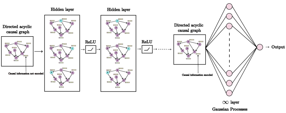
Figure 2: Deep kernel learning while incorporating causal information

GCNs (Kipf and Welling, 2016a) are a type of neural network that aims to generalize convolutional neural networks to work with graph data. In our approach, we use GCNs to incorporate causal information from the causal graph into the deep kernel learning framework. Let us denote a graph as $G=(V,E)$, where $V$ is the set of vertices (or nodes) and $E\subseteq$ $V\times V$ is the set of edges connecting the vertices. Each node $v\in V$ can have associated features, represented as a vector $x_{v}$, which in our case are the time series data of the variables. The entire graph can thus be represented by a feature matrix $M\in\mathbb{R}^{N\times F}$, where $N$ is the number of nodes and $F$ is the number of features per node. Additionally, the structure of the graph is represented by an adjacency matrix $A\in\{0,1\}^{N\times N}$ that encodes the causal structure, where $A_{ij}=1$ if there is a causal effect from node $i$ to node $j$, and 0 otherwise. Assuming $H^{(l)}$ represents the hidden state in the $l$-th layer with $H^{(0)}=M$, $W^{(l)}$ being the weight matrix for the $l$-th layer, $\tilde{A}=A+I$ being the adjacency matrix of the graph $G$ with added self-connections ($I$ is the identity matrix), $\tilde{D}$ being the diagonal node degree matrix of $\tilde{A}$, and $\sigma(\cdot)$ representing a nonlinear activation function, the graph convolution operation in its simplest form can be expressed as:

$$H^{(l+1)}=\sigma\left(\tilde{D}^{-\frac{1}{2}}\tilde{A}\tilde{D}^{-\frac{1}{2}}H^{(l)}W^{(l)}\right).$$

This operation effectively updates each node’s representation by considering its own features and those of its causal predecessors, as defined by the graph structure. The normalization with $\tilde{D}^{-\frac{1}{2}}\tilde{A}\tilde{D}^{-\frac{1}{2}}$ ensures that the scale of the feature representations is maintained, preventing vanishing or exploding gradients during training. By stacking multiple GCN layers, the model can capture higher-order dependencies, allowing it to learn rich feature representations that incorporate causal information.

Figure 3: Deep kernel using GCN

The output of the GCN serves as the input to the GP’s kernel function. By transforming the input features using the GCN, we provide the GP with rich representations that incorporate both the features and the causal information between the input variables. The RBF kernel is then applied to these transformed features. Fig. 2 shows the schematic of a deep kernel learning while encoding causal information. This means that the GCN learns not just the static structure of the graph but also how changes in one part of the graph (e.g., one node or a set of nodes) might influence other parts. Once it’s trained, even though the output graph may structurally resemble the input, it contains a deeper understanding of the causal relationship within the graph. Please refer to Zečević et al. (2021) for further insights into connections between GNNs and structural causal models (SCMs). SCMs are frameworks that combine causal graphs with structural equations to model the relationships between variables. Incorporating these structural equations into predictive models via SCMs offers several advantages over traditional statistical or purely correlational models. Traditional models often rely on correlation between variables, which may not reflect true causal relationships. SCMs on the other hand explicitly model causation, ensuring that the influence of each variable on others is accurately represented. Due to this, models based on causation are more likely to generalize well to new unseen data, especially under interventions or distribution shifts. The predictions remain reliable even when the underlying data distribution changes, as causal relationships are invariant to such changes.

The causal graph for engine-out NOx was constructed based on expert guidance from Cummins, reflecting a physical understanding of how engine-out NOx is caused due to other variables in a diesel compression ignition engine. However, due to intellectual property (IP) protection, we have not shared the graph in this paper. It is important to note that while GCNs incorporate causal graph information into feature representations, they do not perform explicit causal inference or enforce causal constraints in predictions. Instead, it improves the model’s ability to learn complex dependencies by embedding structural information from the causal graph (Thost and Chen, 2021).

3.3 Verifying the approach on an illustrative example

Figure 4: Structural causal model (illustrative example)

To validate our proposed method, we apply it to a synthetic illustrative example based on a predefined SCM. Consider a system with $k$ input variables and one output variable. We denote the input variables as $x_{1},x_{2},\dots,x_{k}$, and the output variable as $y$. Specifically, let $y_{t}$ represent the target variable at time step $t$. The SCM for this example defines the following causal relationships:

$$x_{5} =x_{1}^{2},$$

$$x_{6} =x_{2}\log(1+|x_{4}|)+x_{3},$$

$$x_{7} =\sin(x_{5})\cos(x_{5}),$$

$$x_{8} =x_{6}^{2}+\sqrt{|x_{5}|},$$

$$y =x_{7}+x_{8}.$$

In this model, each equation represents how a child variable is causally influenced by its parent variables. For example, $x_{5}$ is directly influenced by $x_{1}$, while $y$ is directly influenced by $x_{7}$ and $x_{8}$. This hierarchical and nonlinear structure allows us to assess how well our causal graph-enhanced GP captures the underlying causal dependencies and nonlinear relationships within the data, as depicted in Fig 4. To evaluate our approach, we generate synthetic data that adheres to the defined SCM, ensuring the preservation of causal relationships. We begin by sampling the input variables $x_{1,t},x_{2,t},x_{3,t},x_{4,t}$ for each time step $t$ from predefined distributions. Using these sampled inputs, we compute the intermediate variables $x_{5,t},x_{6,t},x_{7,t},x_{8,t}$ according to the SCM equations. The output variable $y_{t}$ is then defined as the sum of $x_{7,t}$ and $x_{8,t}$, with the additive Gaussian noise $\epsilon_{t}\sim\mathcal{N}(0,\zeta^{2})$ to account for measurement uncertainty:

$$y_{t}=x_{7,t}+x_{8,t}+\epsilon_{t}.$$

Furthermore, we model the measured input variables $x_{i,t,\text{meas}}$ with uncertainty by introducing measurement noise:

$$x_{i,t,\text{meas}}\mid x_{i,t}\sim\mathcal{N}\left(x_{i,t},\tau^{2}\right),\quad i=1,2,\dots,k,$$

where $\tau$ denotes the standard deviation. The GP model is then trained to predict $y_{t}$ using the inputs while incorporating the information of the causal graph through the deep kernel. We evaluate the performance of our model by comparing it with a standard GP and a GP equipped with a conventional deep kernel using multilayer perceptron (MLP). Additionally, we assess the predictive accuracy of our model against scenarios where the causal information is either partially correct or entirely incorrect, in order to validate the effectiveness of our approach.

4 Results

4.1 Data Generation

4.1.1 Illustrative example

To generate synthetic data, we set $\zeta=0.01$ and $\tau=0.01$. A total of 10,000 samples are generated, with the first 9000 samples used for training and the last 1000 samples reserved for testing.

4.1.2 Engine-out NOx

Experimental data from a multi-pulse fueling diesel compression ignition engine was provided by Cummins Inc. For the construction of probabilistic models, we elected to utilize the dataset that includes EGR as it covered the entire operating region of the engine. The performance of the trained models is then tested on six different validation datasets that were collected on various duty cycles by intentionally running at varying engine-out NOx levels. In our discourse, we consider the experimental data to be the ground truth and the modeling results are compared with it.

4.2 Input Selection

The input variables for modeling engine-out NOx were chosen primarily on the basis of the physical understanding of how NOx is produced in an engine. Using ARD offers us a certain level of flexibility with our input selections. Essentially, if a chosen input turns out not to be directly relevant, the ARD mechanism will assign a lower weight, minimizing its impact on the model. Therefore, we can be somewhat less stringent in ensuring that every single input is precisely the right one. However, a crucial aspect to monitor when using ARD is the correlation between the input variables. It is important to ensure that the inputs we consider are not correlated to each other which was indeed the case. Due to IP considerations, we have not disclosed the complete list of input variables used in this study. However, we can confirm that the selected inputs include various engine operating parameters related to the air handling system, fuel system, and combustion system, that are known to influence NOx formation.

4.3 Data Normalization

Prior to training the GP model, we normalized all datasets using the empirical cumulative distribution function (ECDF) method. This normalization converts the data into a uniform distribution, which is especially beneficial when the original distribution is unknown or does not conform to the Gaussian distribution often assumed by many machine learning algorithms. Additionally, the ECDF approach improves the robustness to outliers by ranking data points instead of directly scaling their values.

4.4 Metrics

4.4.1 Illustrative example

To compare the efficacy of our proposed model in comparison to a standard GP and a GP with a conventional deep kernel, we use the root mean squared error (RMSE) as the primary performance metric. Additionally, we assess the model’s performance in scenarios with partially correct or entirely incorrect causal information by using RMSE, mean absolute error (MAE), and the coefficient of determination ($R^{2}$) as evaluation metrics.

4.4.2 Engine-out NOx

In order to assess the ability of the GP models to accurately model NOx, we employed several quantitative metrics. These include the RMSE, the 90th, 95th, and 98th percentiles of the absolute errors in NOx emissions, which provide a comprehensive view of the error distribution. These metrics were selected for their robustness in assessing the model accuracy, as they allow us to capture not only the average model performance but also the behavior of the model under various conditions, particularly focusing on extreme values. Additionally, to examine the consistency of NOx emissions under identical input conditions, we used the Quantile-Quantile (Q-Q) plot, which provides a graphical representation of the empirical distribution of the model’s output compared to a theoretical distribution, thereby allowing a thorough assessment of the model’s ability to replicate the observed NOx distribution under repeated experiments.

4.5 Modeling Results

The GP models and deep kernel using GCN are programmed using GPyTorch (Gardner et al., 2018) and PyTorch Geometric (Fey and Lenssen, 2019) library respectively, with a PyTorch backend. We set the loss function as negative of exact marginal log likelihood and the optimizer used is Adam (Kingma, 2014) with tuned hyperparameters. To prevent the models from overfitting, we consider using early stopping with a patience of 50 epochs.

4.5.1 Illustrative example

We train three GP models: the first with a standard RBF kernel (GP (RBF)), the second with a conventional deep kernel using MLP (GP (DRBF-MLP)), and the third with a deep kernel based on GCN (GP (DRBF-GCN)). Table 1 presents the accuracy of the median predictions of these models, evaluated using RMSE as the number of training samples increases. Notably, the GP (DRBF-GCN) outperforms the other two models, especially in low-data regimes (i.e., when $N=1000$) due to the inductive bias introduced by the causal information encoded in the deep kernel. As the number of training samples increases, the performance of all three models improves, and they converge to similar levels of accuracy.

Table 1: Accuracy of the GP models (illustrative example)

Models	RMSE (using N training samples)
	N = 1000	N = 5000	N = 9000
GP (RBF)	0.45	0.20	0.16
GP (DRBF-MLP)	0.54	0.21	0.15
GP (DRBF-GCN)	0.18	0.16	0.15

To further demonstrate that the model effectively encodes causal information, we train three additional GP models: one that encodes the correct causal relationships, one that encodes partially correct causal relationships, and one that encodes incorrect causal relationships. Table 2 shows the accuracy of these model’s median predictions on the test dataset, evaluated using RMSE, MAE, and $R^{2}$. We can see that the best performance is achieved by the model which encoded the correct causal information with the performance degrading progressively as the encoding of causal information becomes partially correct to completely incorrect. This verifies our proposed approach.

Table 2: Accuracy of the GP models with different causal information (illustrative example)

Models	RMSE	MAE	$R^{2}$
Correct causal information	0.15	0.11	0.95
Partially correct causal information	0.52	0.31	0.54
Incorrect causal information	2.31	1.98	-9.68

4.5.2 Engine-out NOx

In our comprehensive analysis of various GP models built for predicting engine-out NOx, we were provided with the readings from an ECM virtual sensor provided by Cummins for the purpose of comparison. This comparative study revealed distinct trends and performance nuances in our models. Firstly, there is a clear indication that increasing the complexity of GP models improves their predictive performance. This is particularly noticeable when comparing the performance of standard GP (RBF) models with different input window sizes against relatively complex models such as GP (Deep RBF) with CNN or GCN. These complex models often outperform both the standard GP models and the ECM virtual sensor provided by Cummins, especially in scenarios with cumulative NOx level 2 (as seen in Tables 3, 4 and 8). However, this trend is not universal across all test cases, suggesting that while complexity contributes to performance, it is not the sole determinant. We can see that GP (DRBF-GCN) [$W_{s}=5s$] performs relatively better than all other models for validation 1, 2, and 6 (see Tables 3, 4 and 8). However, we observe a relatively better performance of more simpler models for cumulative NOx level 1 scenarios (as seen in Tables 6 and 7).

It is important to differentiate between epistemic and aleatory uncertainties in this context. Epistemic uncertainty originates from insufficient knowledge or data within the model, while aleatory uncertainty is due to the inherent variability in the system under study. In the cumulative NOx level 3 scenario of validation 6, all GP models including the more complex ones, underperform significantly compared to the ECM sensor. The ECM sensor’s relatively better performance in this scenario can be linked to its training on a different dataset, likely encompassing a wider representation of NOx conditions with cumulative NOx level 3. This highlights a potential gap in our training dataset for scenarios with cumulative NOx level 3, particularly in terms of epistemic uncertainty. Fig. 5 further supports this, showing considerable epistemic uncertainty as compared to aleatory uncertainty in the GP (DRBF-CNN) [$W_{s}=5$s] model predictions for FTP with cumulative NOx level 3, suggesting encounters with scenarios not adequately captured in the training phase. Due to encoding of causal relationships in the deep kernel for GP (DRBF-GCN), we can observe a relative decrease in the offset between the median prediction and the measured data (Fig. 6) as compared to GP (DRBF-CNN). Although incorporating physical laws did not help us remove the offset completely, it was at least able to decrease this offset compared to pure regression models. Please note that all the values presented in the tables are expressed in parts per million (ppm).

Table 3: Validation 1 (FTP cumulative NOx level 2)

Models	RMSE	NOx Error Percentiles
		90th	95th	98th
GP (RBF) [$W_{s}=1s$]	61.39	75.86	111.10	174.29
GP (RBF) [$W_{s}=2s$]	63.30	68.81	118.17	193.81
GP (RBF) [$W_{s}=3s$]	61.68	73.78	113.68	187.26
GP (RBF) [$W_{s}=4s$]	63.08	80.54	117.73	174.86
GP (RBF) [$W_{s}=5s$]	66.58	77.56	120.20	203.28
GP (DRBF-CNN) [$W_{s}=5s$]	61.46	80.18	120.83	176.45
GP (DRBF-GCN) [$W_{s}=5s$]	60.73	74.58	110.33	170.36
ECM virtual sensor	102.53	142.88	189.14	361.77

Table 4: Validation 2 (RMCSET cumulative NOx level 2)

Models	RMSE	NOx Error Percentiles
		90th	95th	98th
GP (RBF) [$W_{s}=1s$]	46.20	81.78	97.09	105.62
GP (RBF) [$W_{s}=2s$]	46.55	64.25	69.62	91.48
GP (RBF) [$W_{s}=3s$]	42.87	74.09	82.32	86.66
GP (RBF) [$W_{s}=4s$]	44.44	74.90	83.69	86.88
GP (RBF) [$W_{s}=5s$]	45.78	75.07	82.55	85.91
GP (DRBF-CNN) [$W_{s}=5s$]	50.16	83.66	92.35	97.72
GP (DRBF-GCN) [$W_{s}=5s$]	42.86	74.18	82.45	86.95
ECM virtual sensor	58.59	105.38	111.58	140.42

Table 5: Validation 3 (Step cycle cumulative NOx level 2)

Models	RMSE	NOx Error Percentiles
		90th	95th	98th
GP (RBF) [$W_{s}=1s$]	117.62	126.26	185.99	313.48
GP (RBF) [$W_{s}=2s$]	73.70	98.19	141.58	196.38
GP (RBF) [$W_{s}=3s$]	82.45	132.19	175.77	250.93
GP (RBF) [$W_{s}=4s$]	90.24	132.87	183.10	268.93
GP (RBF) [$W_{s}=5s$]	101.43	147.34	197.26	294.08
GP (DRBF-CNN) [$W_{s}=5s$]	81.33	101.54	153.63	254.07
GP (DRBF-GCN) [$W_{s}=5s$]	83.54	103.82	158.26	241.45
ECM virtual sensor	216.60	349.67	561.70	758.07

Table 6: Validation 4 (FTP cumulative NOx level 1)

Models	RMSE	NOx Error Percentiles
		90th	95th	98th
GP (RBF) [$W_{s}=1s$]	89.56	100.05	132.69	199.25
GP (RBF) [$W_{s}=2s$]	80.38	103.20	134.09	169.11
GP (RBF) [$W_{s}=3s$]	77.94	94.85	124.80	171.09
GP (RBF) [$W_{s}=4s$]	77.37	88.78	116.60	148.06
GP (RBF) [$W_{s}=5s$]	83.37	98.78	125.67	152.97
GP (DRBF-CNN) [$W_{s}=5s$]	126.98	209.13	291.76	334.32
GP (DRBF-GCN) [$W_{s}=5s$]	93.71	110.48	143.31	205.34
ECM virtual sensor	152.79	225.43	287.62	400.98

Table 7: Validation 5 (Step cycle cumulative NOx level 1)

Models	RMSE	NOx Error Percentiles
		90th	95th	98th
GP (RBF) [$W_{s}=1s$]	123.90	190.46	247.38	392.68
GP (RBF) [$W_{s}=2s$]	85.35	132.38	177.28	256.68
GP (RBF) [$W_{s}=3s$]	84.83	130.67	189.10	277.71
GP (RBF) [$W_{s}=4s$]	92.76	147.26	212.70	313.76
GP (RBF) [$W_{s}=5s$]	96.39	151.64	229.76	313.40
GP (DRBF-CNN) [$W_{s}=5s$]	89.66	138.24	186.94	265.52
GP (DRBF-GCN) [$W_{s}=5s$]	91.58	143.65	188.63	265.20
ECM virtual sensor	213.85	324.20	510.12	711.17

Table 8: Validation 6 (FTP cumulative NOx level 3)

Models	RMSE	NOx Error Percentiles
		90th	95th	98th
GP (RBF) [$W_{s}=1s$]	438.44	691.64	703.77	731.37
GP (RBF) [$W_{s}=2s$]	473.84	791.03	819.27	848.78
GP (RBF) [$W_{s}=3s$]	345.26	569.79	584.68	616.90
GP (RBF) [$W_{s}=4s$]	289.50	468.79	481.60	515.96
GP (RBF) [$W_{s}=5s$]	285.97	467.26	484.28	527.75
GP (DRBF-CNN) [$W_{s}=5s$]	257.10	399.96	427.23	455.54
GP (DRBF-GCN) [$W_{s}=5s$]	138.18	123.43	183.87	380.44
ECM virtual sensor	107.55	108.35	169.16	349.40

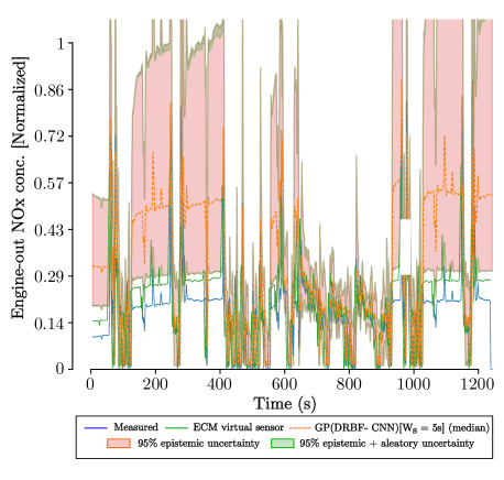
Figure 5: GP(DRBF-CNN)[$W_{s}=5s$] predictions on FTP with cumulative NOx level 3

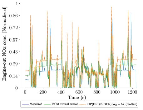
Figure 6: GP(DRBF-GCN)[$W_{s}=5s$] predictions on FTP with cumulative NOx level 3

To analyze the variability of NOx conditioned on the same input, Fig. 7 shows the Q-Q plots between the sample quantiles of the GP (DRBF-GCN) [$W_{s}=5$s] model (in the scaled version) and the theoretical quantiles of standard normal for all validation datasets. In an ideal case these distributions should be the same i.e., all the points must lie on the 45 degree dotted red line. We can see that except for FTP with cumulative NOx level 3, the intermediate NOx values closely follow the standard normal. There is a reasonable difference observed between the sample and theoretical quantiles for extreme low and high NOx values. This is indicative that our model is very sensitive to the changes in input values for predicting extreme low or high NOx values. Due to the gap between validation 6 and the training datasets, we can observe reasonable deviations between these two quantiles for FTP with cumulative NOx level 3. We could not compare these results with the ECM virtual sensor as it was not a probabilistic model.

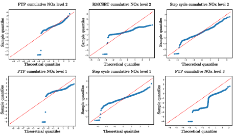
Figure 7: Quantile-Quantile plots (GP(DRBF-GCN)[$W_{s}=5s$])

5 Conclusions

This paper developed and validated a set of probabilistic models for predicting engine-out NOx using GPR. These models were compared against a virtual ECM sensor, providing a robust framework for assessing their predictive performance under different operating conditions. We systematically increased the complexity of the model in three stages: first, by incorporating memory through varying input window sizes; second, by using CNN within the deep kernel framework to improve the model’s ability to learn complex temporal patterns; and finally, by using GCN to incorporate causal information, embedding knowledge informed by physics into the learning process. The key takeaways from the results indicate that increasing model complexity led to improved performance in NOx scenarios with cumulative NOx level 2, with the GP(DRBF-GCN) model consistently outperforming simpler models and the ECM sensor. The incorporation of causal information in the GP(DRBF-GCN) model reduced the offset between predictions and actual measurements for the FTP cycle with cumulative NOx level 3, although performance in extreme NOx cases varied. Simpler models performed better in scenarios with cumulative NOx level 1, and NOx predictions (more specifically, the FTP cycle with cumulative NOx level 3) suffered from high epistemic uncertainty due to insufficient training data.

Although the GP(DRBF-GCN) model demonstrates superior performance in encoding and leveraging causal information for NOx prediction, a significant limitation must be considered. The efficacy of GP(DRBF-GCN) is heavily based on the accuracy of the encoded causal relationships. As illustrated in Table 2, the performance of the model significantly degrades when causal information is partially correct or incorrect, highlighting its sensitivity to the quality of causal encoding. This dependence requires precise identification and integration of causal factors, which may not always be feasible in complex engine systems.

Authors’ contributions

Shrenik Zinage: Methodology, Software, Validation, Visualization, Writing - original draft. Ilias Bilionis: Funding acquisition, Methodology, Validation, Writing - review and editing. Peter Meckl: Funding acquisition, Validation, Writing - review and editing.

Acknowledgement

The authors extend sincere gratitude to Akash Desai from Cummins Inc. for his invaluable feedback and guidance throughout this research. Additionally, heartfelt thanks are due to Dr. Lisa Farrell and Clay Arnett from Cummins Inc., not only for sponsoring this research but also for their crucial technical input and the provision of experimental data essential for conducting the simulations.

Declaration of conflicting interests

The author(s) declared no potential conflicts of interest with respect to the research, authorship, and/or publication of this article.

Funding

This work has been funded by Cummins Inc under grant number 00099056.

References

- Aithal (2010) Aithal S (2010) Modeling of nox formation in diesel engines using finite-rate chemical kinetics. Applied Energy 87(7): 2256–2265.
- Aliramezani et al. (2022) Aliramezani M, Koch CR and Shahbakhti M (2022) Modeling, diagnostics, optimization, and control of internal combustion engines via modern machine learning techniques: A review and future directions. Progress in Energy and Combustion Science 88: 100967.
- Asprion et al. (2013) Asprion J, Chinellato O and Guzzella L (2013) A fast and accurate physics-based model for the nox emissions of diesel engines. Applied energy 103: 221–233.
- Bowman (1975) Bowman CT (1975) Kinetics of pollutant formation and destruction in combustion. Progress in energy and combustion science 1(1): 33–45.
- Calandra et al. (2016) Calandra R, Peters J, Rasmussen CE and Deisenroth MP (2016) Manifold gaussian processes for regression. In: 2016 International joint conference on neural networks (IJCNN). IEEE, pp. 3338–3345.
- Cho et al. (2018) Cho H, Brewbaker T, Upadhyay D, Fulton B and Van Nieuwstadt M (2018) A structured approach to uncertainty analysis of predictive models of engine-out nox emissions. International Journal of Engine Research 19(4): 423–433.
- EPA (2021) EPA (2021) Regulations for emissions from vehicles and engines. URL https://www.epa.gov/regulations-emissions-vehicles-and-engines/cleaner-%****␣main.bbl␣Line␣50␣****trucks-initiative.
- Fang et al. (2022) Fang X, Zhong F, Papaioannou N, Davy MH and Leach FC (2022) Artificial neural network (ann) assisted prediction of transient nox emissions from a high-speed direct injection (hsdi) diesel engine. International Journal of Engine Research 23(7): 1201–1212.
- Fey and Lenssen (2019) Fey M and Lenssen JE (2019) Fast graph representation learning with pytorch geometric. arXiv preprint arXiv:1903.02428 .
- Gardner et al. (2018) Gardner J, Pleiss G, Weinberger KQ, Bindel D and Wilson AG (2018) Gpytorch: Blackbox matrix-matrix gaussian process inference with gpu acceleration. Advances in neural information processing systems 31.
- Gordon et al. (2023) Gordon D, Norouzi A, Blomeyer G, Bedei J, Aliramezani M, Andert J and Koch CR (2023) Support vector machine based emissions modeling using particle swarm optimization for homogeneous charge compression ignition engine. International Journal of Engine Research 24(2): 536–551.
- Guo et al. (2017) Guo C, Pleiss G, Sun Y and Weinberger KQ (2017) On calibration of modern neural networks. In: International conference on machine learning. PMLR, pp. 1321–1330.
- Heywood (2018) Heywood JB (2018) Internal combustion engine fundamentals. McGraw-Hill Education.
- Kingma (2014) Kingma DP (2014) Adam: A method for stochastic optimization. arXiv preprint arXiv:1412.6980 .
- Kipf and Welling (2016a) Kipf TN and Welling M (2016a) Semi-supervised classification with graph convolutional networks. arXiv preprint arXiv:1609.02907 .
- Kipf and Welling (2016b) Kipf TN and Welling M (2016b) Variational graph auto-encoders. arXiv preprint arXiv:1611.07308 .
- Lavoie et al. (1970) Lavoie GA, Heywood JB and Keck JC (1970) Experimental and theoretical study of nitric oxide formation in internal combustion engines. Combustion science and technology 1(4): 313–326.
- LeCun et al. (2015) LeCun Y, Bengio Y and Hinton G (2015) Deep learning. nature 521(7553): 436–444.
- Li et al. (2015) Li Y, Tarlow D, Brockschmidt M and Zemel R (2015) Gated graph sequence neural networks. arXiv preprint arXiv:1511.05493 .
- Scarselli et al. (2008) Scarselli F, Gori M, Tsoi AC, Hagenbuchner M and Monfardini G (2008) The graph neural network model. IEEE transactions on neural networks 20(1): 61–80.
- Shahpouri et al. (2021) Shahpouri S, Norouzi A, Hayduk C, Rezaei R, Shahbakhti M and Koch CR (2021) Soot emission modeling of a compression ignition engine using machine learning. IFAC-PapersOnLine 54(20): 826–833.
- Shin et al. (2020) Shin S, Lee Y, Kim M, Park J, Lee S and Min K (2020) Deep neural network model with bayesian hyperparameter optimization for prediction of nox at transient conditions in a diesel engine. Engineering Applications of Artificial Intelligence 94: 103761.
- Thost and Chen (2021) Thost V and Chen J (2021) Directed acyclic graph neural networks. arXiv preprint arXiv:2101.07965 .
- Veličković et al. (2017) Veličković P, Cucurull G, Casanova A, Romero A, Lio P and Bengio Y (2017) Graph attention networks. arXiv preprint arXiv:1710.10903 .
- Williams and Rasmussen (2006) Williams CK and Rasmussen CE (2006) Gaussian processes for machine learning, volume 2. MIT press Cambridge, MA.
- Wilson et al. (2016) Wilson AG, Hu Z, Salakhutdinov R and Xing EP (2016) Deep kernel learning. In: Artificial intelligence and statistics. PMLR, pp. 370–378.
- Xu et al. (2018) Xu K, Hu W, Leskovec J and Jegelka S (2018) How powerful are graph neural networks? arXiv preprint arXiv:1810.00826 .
- Yousefian et al. (2021) Yousefian S, Bourque G and Monaghan RF (2021) Bayesian inference and uncertainty quantification for hydrogen-enriched and lean-premixed combustion systems. international journal of hydrogen energy 46(46): 23927–23942.
- Zečević et al. (2021) Zečević M, Dhami DS, Veličković P and Kersting K (2021) Relating graph neural networks to structural causal models. arXiv preprint arXiv:2109.04173 .
- Zinage et al. (2024a) Zinage S, Mondal S and Sarkar S (2024a) Dkl-kan: Scalable deep kernel learning using kolmogorov-arnold networks. arXiv preprint arXiv:2407.21176 .
- Zinage et al. (2024b) Zinage V, Zinage S, Bettadpur S and Bakolas E (2024b) Leveraging gated recurrent units for iterative online precise attitude control for geodetic missions. arXiv preprint arXiv:2405.15159 .