Quantitative control on the Carleson -function determines regularity
Abstract.
Carleson’s -conjecture states that for certain planar domains, points on the boundary where tangents exist can be characterized in terms of the behavior of the -function. This conjecture, which was fully resolved by Jaye, Tolsa, and Villa in 2021, established that qualitative control on the rate of decay of the Carleson -function implies the existence of tangents, up to a set of measure zero. In this paper we prove that quantitative control on the rate of decay of this function gives quantitative information on the regularity of the boundary.
1. Introduction
In this paper we continue the study, which began in [Bis87, BCGJ89, JTV21], of the relationship between the regularity of certain planar curves and the rate of decay of the Carleson -function. Geometric functions and their relationship to the regularity of sets has been the focus of many works over the past four decades, beginning in [Jon90, DS91]. In particular, a geometric function measuring, in some sense, how well the boundary of a domain cuts circles in half appeared in [Bis87]. This function is known as the Carleson -function.
Definition 1.1 (Carleson -function).
Let be Jordan domain, i.e. a domain whose boundary is a Jordan curve, and let . Let denote the largest open arc (with respect to -measure) on the circumference contained in . Define
Carleson conjectured that for certain planar domains, points on the boundary where tangents exist could be characterized in terms of a Dini-type control on this function.
Conjecture 1 (Carleson’s -conjecture).
Suppose is a Jordan curve. Except for a set of zero -measure, is a tangent point of if and only if
| (1) |
The “only if” direction of the conjecture is well-known, see for instance [Bis87, BJ94, GM05]. The converse direction was open for more than thirty years, only recently being resolved by Jaye, Tolsa, and Villa in [JTV21].
In [Jon90], Jones introduced another geometric function, known as the Jones -numbers. The Jones -numbers measure how far the set deviates from a plane inside a ball.
Definition 1.2 (Jones -numbers).
Let be closed. For and ,
Conjecture 1, after being fully establised by [JTV21], gives a characterization of the tangent points of Jordan domains, up to a set of measure zero. In [BJ94], the authors proved an analogous result to Conjecture 1 in terms of the -numbers. In [DKT01], the authors proved that having quantitative control on the rate of decay of the -numbers provides quantitative information about the regularity of .
Proposition 1 (Proposition 9.1, [DKT01]).
Let be given. Suppose that is a Reifenberg-flat set with vanishing constant of dimension in (see definition 1.4), and that for each compact set there exists a constant such that
| (2) |
Then is a -submanifold of dimension in .
We state this result for -dimensional sets in , although the result in [DKT01] is proved in higher dimensions. In general, it is known that the behavior of the -numbers determine the regularity of a given set, see [Jon90, DS91, Oki92, Ghi20, DNI22]. It is then natural to wonder, to what extent does the behavior of the -function determine the regularity of a given set? In this paper, we prove an analogous result to Proposition 1 involving the Carleson -function. Our main result is the following theorem.
Theorem 1.
Let be a Jordan domain and . Let . Fix some and . Suppose there exists such that
| (3) |
then is a -manifold of dimension in .
In Proposition 1, the authors assume an additional hypothesis, that the set is a Reifenberg-flat set with vanishing constant, which we omit. In [DKT01], the sets considered are more general, and this assumption ensures that has no holes.
Definition 1.3 (Bilateral -numbers).
For and , set
| (4) |
where
and denotes the set of all -dimensional subspaces of .
Definition 1.4 (Reifenberg-flat set with vanishing constant).
Let . Following [DKT01], a closed set is -Reifenberg-flat of dimension if for all compact sets there is a radius such that
is a Reifenberg-flat set with vanishing constant if for every compact set ,
The Carleson -function is not continuous with respect to nor , and is therefore not stable enough to apply the techniques that have been used to relate the behavior of the -numbers to the regularity of a given set. See for instance the discussion in [DS91, p.141]. To emphasize the difference between the -function and the -numbers, we give the following example. Suppose is an exponential spiral. At the origin but , since -function takes a measurement of the boundary on circular shells and the -numbers take a measurement of the boundary inside balls. See Figure 2. It is true that if is a tangent point for , then controls up to a multiplicative constant for , see [JTV21].
In order to prove Theorem 1, we prove that is a Reifenberg-flat set with vanishing constant and (2) holds with . Then [DKT01, Proposition 9.1] gives our result. With the discussion above in mind, we remark that the majority of the work in this paper is in proving that the hypothesis on the -function in (3) gives control on the -numbers like in (2). We prove this control, along with the vanishing Reifenberg-flatness, in two lemmas.
Lemma 1.
Let be a Jordan domain and . Let . Fix some and . Suppose there exists such that
Fix and . Then, there exists a line through such that
| (5) |
Lemma 2.
Let be a Jordan domain and . Let . Fix some and . Suppose there exists such that
Fix and . Then, there exists a line through such that
| (6) |
Lemma 1 and Lemma 2 together yield that satisfies the flatness hypothesis necessary to apply Proposition 9.1 in [DKT01]. Moreover, Lemma 2 gives the necessary decay on the -numbers. The proof of Theorem 1 is then a straightforward application of [DKT01, Proposition 9.1].
In Section 2, we prove a general consequence of the assumption on . In Section 3 we prove Lemma 1 in several steps, each step its own lemma. In Section 4 we prove Lemma 2.
Acknowledgments. The author would like to thank Tatiana Toro for being a source of constant support and guidance, Max Goering for his feedback on early drafts of this paper, and Sarafina Ford for her generosity and expertise in tikz.
2. Preliminaries
Since , for all and , for each such and there exist (connected) arcs such that
| (7) |
Thus the situation on is very rigid, in the sense that the portion of this circumference that is not covered by either or has length at most , and since are connected, the location where intersects this circumference is tightly controlled. We make this idea rigorous in the next lemma.
Lemma 3 (Trapped Boundary Lemma).
Fix and . If , let denote the shortest arc on with endpoints and . Then
| (8) |
Proof.
Since are fixed throughout the proof, we drop the dependence on them from the notation. We have the following two cases:
-
(i)
Suppose and .
-
(ii)
Suppose, without the loss of generality, .
First suppose that and . Then,
and
It then follows immediately that
which implies that
Now suppose that . Since , is the largest connected component on and connected, it follows that , and
Since is the shortest arc,
∎
Lemma 3 is crucial in the proofs of both Lemma 1 and Lemma 2 and also yields the following corollary.
Corollary 1 (Line Choice).
Suppose . Let denote the line determined by and , and let be the line determined by and . Then,
Proof. Let such that . Let and denote the shortest arcs on with endpoints , and ,, respectively. From Lemma (3) either or , and the corollary follows.
Definition 2.1 (Good Approximating Line).
Fix and . For any , we call a good approximating line at scale for at .
3. Proof of Lemma 1
To prove Lemma 1, it is sufficient to find a dyadic collection of points on the line , which we denote for coherence in the argument, so that for each point in the collection, there is a boundary point sufficiently close by. The idea, is that as long as the dyadic collection can be taken at a fine enough scale, then every point in the line is close to a dyadic point, which is, in turn, close to the boundary. We begin by showing that at the first dyadic scale, scale , there is a boundary point close by.
Lemma 4 (Half-Scales Lemma).
Let be the same absolute constant as in (3). Fix and . Let , and let . Let be the midpoint of the segment between and on , that is
Then, there exists a point such that
| (9) |
and
| (10) |
Moreover,
| (11) | ||||
where denotes the line through and , and denotes the line through and , and is a constant depending only on .
Remark 1.
Observe that the conclusions of Lemma 4, tell us that
| (12) |
Proof.
Assume (by rotating and translating if necessary) that , is the horizontal axis, and . Consider and . These balls intersect at two points, say and . Note we can conclude that are not boundary points using the Trapped Boundary Lemma since for . The same holds for . Thus, we can assume without the loss of generality that and .
The line segment between and is connected, and thus there must be exist some point, . We claim that this point is “close” to , and in particular, that , where
Suppose not. That is,
| (13) |
Consider , where . To contradict the Trapped Boundary Lemma we will show
| (14) |
Let be the angle between the radius and the line segment .
Observe that
where the first inequality follows from (13) and the last from the fact that . Moreover, since the furthest can be from is , we also have . Thus,
Using the Taylor series for for near we see that
Since , it follows that
| (15) | ||||
where we use the fact that in the final two inequalities. Thus we have obtained the right-hand side inequality in (14). To obtain the left-hand side inequality, it is only necessary to take sufficiently small (which in turn means that is also sufficiently small). Indeed, choosing , then
| (16) |
Thus (15) and (16) yield (14), which contradicts the Trapped Boundary Lemma for the boundary point at scale . Thus, we conclude that , as claimed.
Let . Since , we have that
| (17) |
Using the Taylor expansion for , it is clear that for small enough
and thus
| (18) |
Remark 2.
For in Lemma 4, note that
The result of the Half-Scales Lemma gives the following set up. The points, , on and , constructed above, form an isosceles triangle with height, base angles, and side lengths controlled by the hypothesis on the -function in (3).
We can now iterate the Half-Scales Lemma to obtain the next lemma. Before we can state that lemma precisely, we must introduce some new notation.
For odd, define
where we take , for any . Note that by requiring to be odd, the sub-index must be the generation in which the right endpoint of the segment, , was constructed. The super-index is the super-index of the left-endpoint when relabeled to be in generation . Put another way, the line segments, , are notated based on the generation in which they are constructed. Denote by the point on such that
| (19) |
where is the length of .
Remark 3.
Note that this notation is consistent with the Half-Scales Lemma, where we chose to be the point such that , where , , and .
We now state the lemma.
Lemma 5 (Dyadic Scales Lemma).
Let be the same absolute constant as in (3). Recall, and are fixed. Let , and let , as in the Half-Scales Lemma. Fix . Then for each there exists a point such that
| (20) |
where is a constant depending only on and and the are defined as above.
This lemma is proved in several steps. In Lemma 6 we iteratively apply the Half-Scales Lemma to find points in at the appropriate scale. The goal is to then prove that each is very close to a dyadic point, , in . This is proved in two steps. In Lemma 7 we prove that dyadic points on the base of any triangle constructed in the Half-Scales Lemma is close to an “intermediate” dyadic point on one of the sides of that triangle. In Lemma 8 we iterate Lemma 7 to prove that the dyadic point we started with on , , is close to the midpoint of , , which we know is close to from the Half-Scales Lemma.
Lemma 6.
Fix . There exists a collection of points such that for each odd, is an isosceles triangle with side lengths
satisfying
| (21) | ||||
Moreover, the base angles, of satisfy the following bound:
| (22) |
Lastly,
Proof of Lemma 6.
We build this collection inductively. Let , , and , be as in the statement of the Dyadic Scales Lemma. The case follows from the Half-Scales Lemma with , where and .
Suppose for some there exists a collection of points, , for which the conclusion of Lemma 6 holds.
We now show that we can find a collection of points so that Lemma 6 holds. We begin by relabeling ,
see Figure 8, for example. For each odd, apply the Half-Scales Lemma to , the line segment with endpoints and , to obtain a point such that , which denotes the triangle formed by , , and , is an isosceles triangle with side lengths
such that
Moreover,
Since
follows directly from the Half-Scales Lemma, the lemma is complete. ∎
It may seem worrisome that the bounds in the previous lemma depend on , but for a fixed , the are uniformly bounded in .
Remark 4.
Observe that at generation of the construction, there are applications of the Half-Scales Lemma, and for each odd, there are possibly different values of . But, taking , it follows from an induction argument that these quantities are bounded uniformly in ,
| (23) |
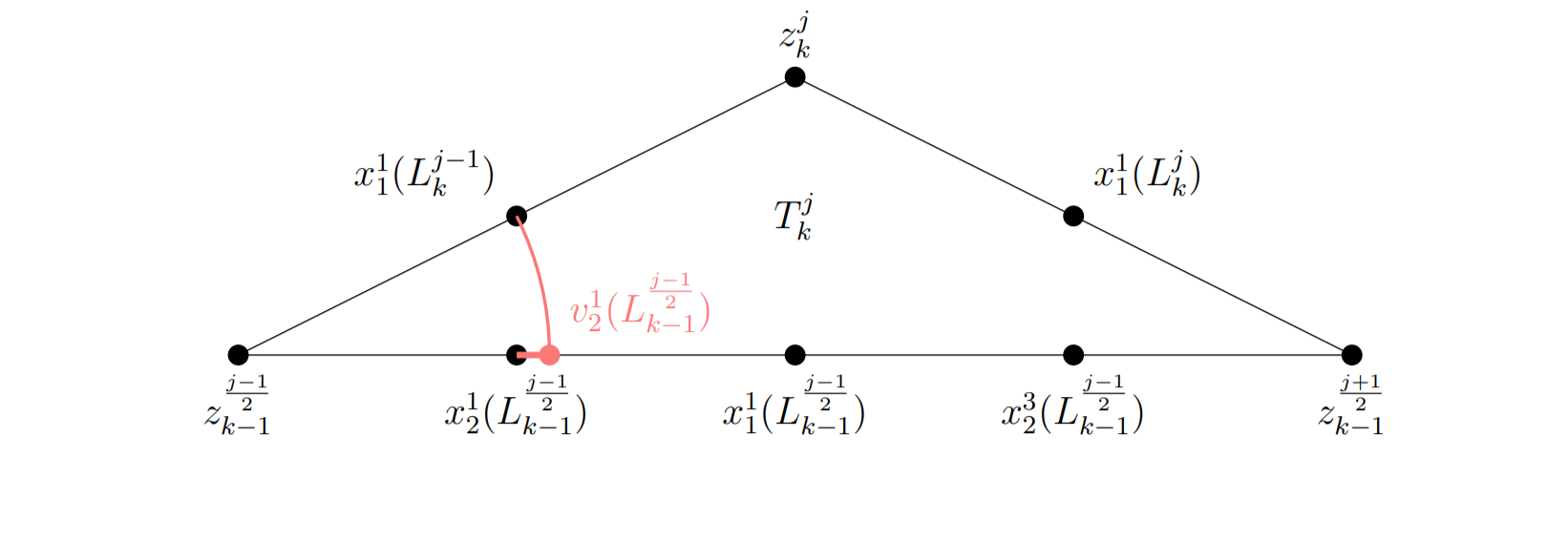
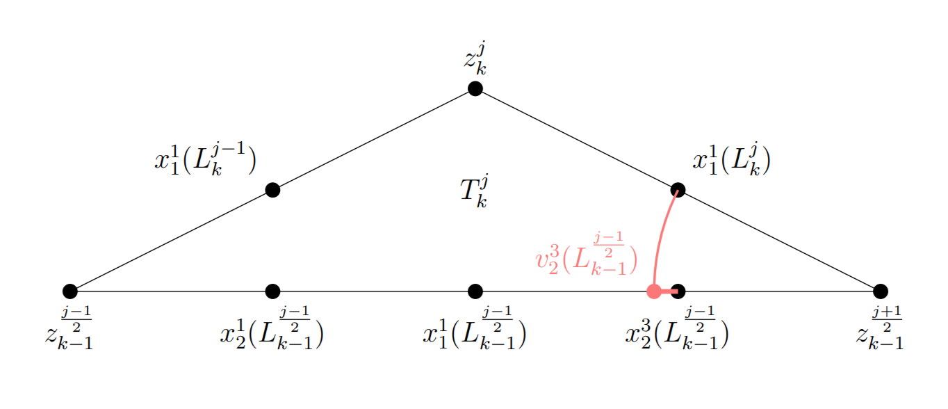
Lemma 7.
Fix . For some odd, let denote the isosceles triangle from Lemma 6. Take the dyadic collection of points on each side of :
(Recall the notation in (19).)
Fix . Then for each with ,
| (24) | ||||
where .
Proof of Lemma 7.
Fix and first suppose that . Let be as in (19) and let be the point in such that
See Figure 10. Then,
where the second to last inequality follows from (22). Furthermore,
where the last inequality follows from (21). Thus from the triangle inequality we have
which together with (23) gives (24). Observe that the case where is similar, but we include the proof below for completeness.
Then,
where the second to last inequality follows from (22). Furthermore,
where the last inequality follows from (21). Thus from the triangle inequality we have
Thus, Lemma 7 is shown.
∎
The idea for the remaining argument is as follows. From the Half-Scales Lemma, the point is very close to . So in order to show (20), a necessary next step is to iterate Lemma 7 to show that
for some constant depending only on and . This means that for each dyadic point in , we need to keep track of the family of dyadic points that satisfy (24) in each successive application of Lemma 7, if we start with . In other words, we need to track which side of the triangle contains the closest dyadic point in each iteration of Lemma 7, to ensure that ’s closest point after iterations is in fact on . To do this, we need to introduce new notation.
Denote and define
where
The function if is closest to the left side of the triangle and if is closest to the right side of the triangle, and thus gives you the “line address” of the closest dyadic point to after iterations.
Lemma 8.
Fix and . Consider the point in the dyadic partition on such that is odd. For , we have
where is the number of iterations.
In particular,
Before proving Lemma 8, we need to prove a counting lemma.
Lemma 9.
Fix . For any and
Proof of Lemma 9.
∎
Proof of Lemma 8.
Fix and . We first prove that
by induction on .
The case of follows immediately from Lemma 7.
Now suppose that for some with
Applying Lemma 7 to with
from Lemma 9, we obtain
Thus, the result follows from the triangle inequality So for any ,
as desired. Moreover, since both
and , Lemma 8 follows.
∎
Proof of Lemma 5.
We are now ready to prove Lemma 1.
Proof of Lemma 1.
Fix to be the smallest natural number such that . Then, for any between and , there exists with , such that
By Lemma 8, there exists a point such that
and then from the triangle inequality,
Thus we have shown that for any between and , .
Lemma 5 can be applied with , the line through and , where . Since
see Corollary 1, it follows that for between and ,
We now show that . Consider a point , where we assume by translating that . From our work above, there exists a point such that
Then,
So for any , . If , let . Observe that . Then,
Our proof of Lemma 1 is complete.
∎
4. Proof of Lemma 2
Our goal in this section is to prove Lemma 2, which we restate below for the reader’s convenience.
Lemma 2.
Let be a Jordan domain. Let and assume . Let . Fix some and . Suppose there exists such that
| (25) |
Fix and . Then, there exists a line through such that
| (26) |
We prove Theorem (2) by contradiction. If there is some boundary point away from inside of , using Lemma 1, we can show that there is a circumference that intersects the boundary near both of these lines, contradicting the Trapped Boundary Lemma.
Proof of Lemma 2.
Suppose for contradiction that there exists a point . Observe that
| (27) |
and let denote the line through and . Taking , the ball .
Let denote the point on between and . Applying Lemma 1 to , , and , we obtain the existence of a point such that
Taking , it follows from the triangle inequality that
| (28) |
Let . The ball contains on its boundary and taking we have .
We claim that is close to . Let denote the minimal arc on between and and let . Then
where . Using the Taylor series for with small enough yields
where .
It then follows from the Trapped Boundary Lemma that for any , we have
| (29) |
Define
the annular region around the circumference , which contains , with radius . intersects in four points, , , labeled counterclockwise such that
We claim that
| (30) |
where and are the minimal arcs between and , and between and , respectively, on . Observe that .
From (29), it is sufficient to show that
Let . Then or , and thus to prove (30), it is sufficient to prove
| (31) |
Consider the triangle with vertices , , and , as seen in blue in Figure 15. We first prove . The law of cosines gives
where depend only on and 111 and . Thus,
and since is close to ,
where are different from above but still depend only on .
Using (28),
where depends only on and . Since
for (31) follows. So, . Moreover, . Since both and contain a boundary point, e.g. or its antipodal point, it must be the case that and , or vice versa. Suppose without the loss of generality that and .
The computations to prove that are similar since
so we omit them here. Thus, and .
Let . It follows from Lemma 5 that there exists a point such that . In particular this means that
and thus,
Since and are in complementary domains, there must exist a point by connectivity.
We will contradict the Trapped Boundary Lemma, i.e. we show that
| (32) |
where is the minimal arc between and on . From the triangle inequality,
| (33) | ||||
So to prove (32), we bound each of the terms, ,, and .
Denote the minimal angle between and by so that
Since , we have and thus,
| (34) |
Let denote the angle such that
Since , using a Taylor series approximation for with small, we have , and thus,
| (35) |
Let denote the angle such that
Then, , and since , we have , where depends only on and . Again using a Taylor series approximation for yields
| (36) |
Thus, applying these estimates to (33) gives
which, for small enough, is clearly smaller than . Thus, the upper bound in (32) holds. It is left to verify the lower bound. Again we apply the estimates to (33), with small enough depending on , and ,
For ,
Thus, (32) holds, and this completes the proof.
∎
References
- [BCGJ89] C. J. Bishop, L. Carleson, J. B. Garnett, and P. W. Jones. Harmonic measures supported on curves. Pac. J. Math., 138(2):233–236, 1989.
- [Bis87] Christopher James Bishop. Harmonic measures supportedon curves. Doctoral dissertation, The University of Chicago, 1987.
- [BJ94] Christoper James Bishop and Peter W. Jones. Harmonic measure, -estimates and the schwarzian derivative. Journal d’analyse mathématique, 62:77–113, 1994.
- [DKT01] Guy David, Carlos Kenig, and Tatiana Toro. Asymptotically optimally doubling measures and Reifenberg flat sets with vanishing constant. Communications on Pure and Applied Mathematics: A Journal Issued by the Courant Institute of Mathematical Sciences, 54:385–449, 2001.
- [DNI22] Giacomo Del Nin and Kennedy Obinna Idu. Geometric criteria for -rectifiability. J. Lond. Math. Soc., II. Ser., 105(1):445–468, 2022.
- [DS91] Guy David and Stephen Semmes. Singular integrals and rectifiable sets in : au-delà des graphes Lipschitziens. Astérisque, (193):7–145, 1991.
- [Ghi20] Silvia Ghinassi. Sufficient conditions for parametrization and rectifiability. Ann. Acad. Sci. Fenn., Math., 45(2):1065–1094, 2020.
- [GM05] John B. Garnett and Donald E. Marshall. Harmonic measure, volume 2 of New Math. Monogr. Cambridge: Cambridge University Press, 2005.
- [Jon90] Peter W. Jones. ectifiable sets and the traveling salesman problem. Inventiones mathematicae, 102:1–15, 1990.
- [JTV21] Benjamin Jaye, Xavier Tolsa, and Michele Villa. A proof of carleson’s -conjecture. Annals of mathematics, 194(1), 2021.
- [Oki92] Kate Okikiolu. Characterization of subsets of rectifiable curves in . Journal of the London Mathematical Society, 2:336–348, 1992.